Fast and Feature-Complete Differentiable Physics Engine for Articulated Rigid Bodies with Contact Constraints

Abstract

We present a fast and feature-complete differentiable physics engine that supports Lagrangian dynamics and contact constraints formulated as linear complementarity programs (LCPs) for articulated rigid body simulation. Our differentiable physics engine offers a complete set of features typically available in existing non-differentiable physics simulators commonly used by robotics applications. We present efficient and novel analytical gradients through the LCP formulation of inelastic contact (without casting it as a QP), complex contact geometry, and continuous-time elastic collision. We show that an implementation of this combination in an existing physics engine (DART) is capable of a 48x single-core speedup over finite-differencing in computing analytical Jacobians for a single timestep, while preserving all the expressiveness of original DART.

1 Introduction

With the rise of deep learning, interest in differentiable physics engines has grown for applications from optimal control to policy learning to parameter estimation. While many differentiable physics engines have been proposed in the recent years and pitched to the robotics community, none so far has replaced commonly used physics engines (bullet; todorov2012mujoco; dart; drake), which offer a complete set of features for forward simulating complex articulated rigid body systems, albeit being non-differentiable.

Physics engines for robotic applications has a set of desired requirements including representing states in the generalized (reduced) coordinates and solving constraint satisfaction problems for contact and other mechanical constraints. Feature-complete forward physics engines with such capabilities have been validated and stress-tested by a large number of users across multiple communities (osrf-website; openAI; opensim). An ideal differentiable physics engine should neither compromise these requirements nor reinvent the forward simulation process in exchange for differentiability. It should also support the entire feature set of an existing physics engine, including various joint types, different actuation mechanisms, and complex contact geometry. Above all, it must be computationally efficient, preferably faster than the forward simulation, such that real-time control and identification problems on complex robotic platforms can be enabled.

In this paper, we take an existing engine commonly used in robotics and graphics communities and make it differentiable. Our engine supports all features available to the forward simulation process so the existing code and applications will remain compatible but enjoying new capabilities enabled by differentiablity. We extend a fast, stable physics engine, DART, to compute analytical gradients in the face of hard contact constraints. By introducing an efficient method for LCP differentiation, contact geometry algorithms, and continuous time approximation for elastic collisions, our engine is able to compute gradients at microseconds per step, much faster than [Karen: quantify it] existing differentiable physics engines with hard contact constraints.

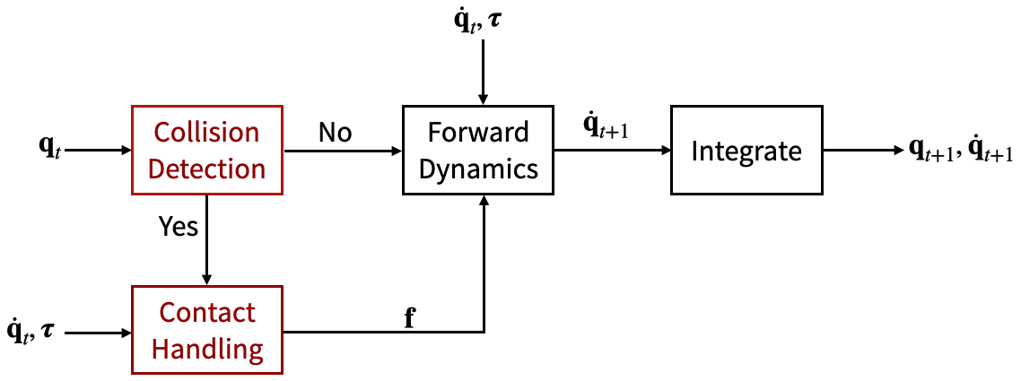
Figure 1: A typical forward simulation at the current state ($\bm{q}_{t},\dot{\bm{q}}_{t}$). The processes shown in red are non-differentiable, namely Collision Detection and Contact handling. [Keenon: Technically the engine integrates forward dynamics of $\dot{q}_{t+1}$, then solves for collision and updates $\dot{q}_{t+1}$, rather than the other way around]

A physics engine that employs hard contact constraints is non-differentiable. While this statement is true, a more interesting question is whether the ”gradient” we manage to approximate in the face of non-differentiability is of any use for the downstream tasks of interest, such as optimal control or system identification? A typical forward simulation involves Collision Detection, Contact Handling, Forward Dynamics and Integration in each discretized timestep illustrated in Figure 1. Non-differentiability arises at Collision Detection and Contact Handling. The contact handling based on solving a LCP is theoretically differentiable with well-defined gradients, except for a subspace in which the contact state switches from static to sliding or to breaking. We show that two well-defined subgradients exist and heuristically selecting one leads to well behaved optimization [Karen: Need results to support this]. On the other hand, collision detection essentially creates a branch which results in non-differentiable $\frac{\partial\bm{f}}{\partial\bm{q}}$, where $\bm{f}$ is the contact force and $\bm{q}$ is the current state of the system. We assume that an infinitesimally small $\bm{\epsilon}$ can be added to $\bm{q}$ without changing the state of branch. This assumption is reasonable because a small amount of penetration always exists at the moment a contact point is detected due to the discretized time in a physics engine. Making such an assumption allows us to compute well-defined gradient and, more importantly, we show that, the gradients computed based on these assumptions do not negatively impact the convergence of optimization.

To summarize, our contributions are as follows:

• A novel and fast method for local differentiability of LCPs without needing to reformulate as QPs, which gives us efficient gradients through static and sliding contacts and friction without changing traditional forward-simulation formulations.

• Fast geometric analytical gradients through 3D contact detection algorithms, which we believe are also novel.

• A novel analytical approximation of continuous time gradients through 3D bounces, which otherwise can lead to errors in discrete time systems.

• A careful, open source implementation of all of our proposed methods (along with analytical gradients through Featherstone first described in GEAR (kim2012lie)) in an open-source fork of the DART physics engine. We have created a pip install package for ease of use.

2 Related Work

Engine	Contact	Dynamics	Collision	Gradients
MuJoCo (todorov2012mujoco)	Customized	Generalized coord	Complete	Finite Diff
(degrave2019differentiable)	Impulse-based	Cartesian coord	Primitives	Auto Diff
DiffTaichi (difftaichi)	Impulse-based	Caresian coord	Primitives	Auto Diff
Tiny (heiden2020augmenting)	Interative LCP	Generalized coord	Primitives	Auto Diff
(de2018end)	Direct LCP	Cartesian coord	Primitives	Symbolic Diff
ADD (geilinger2020add)	Customized	Generalized coord	Primitives	Symbolic Diff
DiffDart	Direct LCP	Generalized coord	Complete	Symbolic Diff

Table 1: Trade off comparison of published differentiable physics engines

Differentiable physics simulation has been investigated previously in many different fields, including mechanical engineering , robotics , physics and computer graphics (jovn2000). Enabled by recent advances in automatic differentiation methods and libraries , a number of differentiable physics engines have been proposed to solve control and parameter estimation problems for rigid bodies and non-rigid bodies . While they share similar high-level goal of solving ”inverse problems”, the features and functionality provided by these engines vary widely, including the variations in contact handling, state space parameterization and collision geometry support. Table LABEL: highlights the differences in a few differentiable physics engines that have demonstrated the ability to simulate articulated rigid bodies with contact. Based on the functionalities each engine intends to support, the approaches to computing gradients can be organized in following categories.

Finite-differencing is a straightforward way to approximate gradients of a function. For a feature-complete physics engine, finite-differencing is ideal because it bypasses all the complexity of forward simulation process from which gradients are difficult to obtain analytically. For example, a widely used physics engine, MuJoCo (todorov2012mujoco), supports gradient computation via finite differencing. However, finite-differencing tends to introduce round-off errors and performs poorly for a large number of input variables. [Karen: provide performance comparison between DiffDart and MuJoco?]

Automatic differentiation (auto-diff) is a method for computing gradients of a sequence of elementary arithmetic operations or functions automatically. However, constraint satisfaction required by many existing, feature-complete robotic physics engines is not supported by auto-diff libraries. To avoid this issue, many recent differentiable physics engines instead implement impulse-based contact handling, which could lead to numerical instability if the contact parameters are not tuned properly for the specific dynamic system and the simulation task. Degrave et al. implemented a rigid body simulator in the Theano framework , while DiffTaichi implemented a number of differentiable physics engines, including rigid bodies, using Taichi programming language , both representing dynamic equations in Cartesian coordinates and handling contact with impulse-based methods . In contrast, Tiny Differentiable Simulator models contacts as a LCP, but they solve the LCP iteratively via Projected Gauss Siedel (PGS) method , instead of directly solving a constraint satisfaction problem, making it possible to compute gradient through auto-diff.

Symbolic differentiation is another way to compute gradients by directly differentiate mathematical expressions. For complex programs like Lagrangian dynamics with constraints formulated as a Differential Algebraic Equations, symbolic differentiation can be exceedingly difficult. Earlier work computed symbolic gradients for smooth dynamic systems . Symbolic differentiation becomes manageable when the gradients are only required within smooth contact modes (Toussaint-tool) or a specific contact mode is assumed (song-push). Recently, Amos and Kolter proposed a method, Opt-Net, that back-propagates through the solution of an optimization problem to its input parameters (amos2017optnet). Building on Opt-Net, de Avila Belbute-Peres et al. (de2018end) derived analytical gradients through LCP formulated as a QP. Their method enables differentiability for rigid body simulation with hard constraints, but their implementation represents 2D rigid bodies in Cartesian coordinates and only supports collisions with a plane, insufficient for simulating complex articulated rigid body systems. More importantly, computing gradients via QP requires solving a number of linear systems which does not take advantage of sparsity of the LCP structure [Karen: Need to verify this by math]. Qiao et al. (Qiao:2020) built on (amos2017optnet) and improved the performance of contact handling by breaking a large scene to smaller impact zones. A QP is solved for each impact zone to ensure that the geometry is not interpenetrating, but contact dynamics and conservation laws are not considered. Solving contacts for localized zones has been previously implemented in many existing physics engines (todorov2012mujoco; bullet; dart). Adapting the collision handling routine in DART, our method by default utilizes the localized contact zones to speed up the performance. Adjoint sensitivity analysis has also been used for computing gradients of dynamics. Millard et al.(Millard:2020) combined auto-diff with adjoint sensitivity analysis to achieve faster gradient computation for higher-dof systems, but their method did not handle contact and collision. Geilinger et al. analytically computed derivatives through adjoint sensitivity analysis and proposed a differentiable physics engine with implicit forward integration and a customized frictional contact model that is natively differentiable.

Approximating physics with neural networks is a different approach towards differentiable physics engine. Instead of forward simulating a dynamic system from first principles of Newtonian mechanics, a neural network is learned from training data. Examples of this approach include Battaglia et. al (battaglia2016interaction), Chang et. al. (chang2016compositional), and Mrowca et. al (mrowca2018flexible).

DiffDart also employs symbolic differentiation to compute gradients. Like Like Tiny Differentiable Simulator, its forward simulation integrates Lagrangian dynamics in generalized coordinates and solves for constraint forces via a LCP. However, DiffDart directly solves for LCP rather than employing an iterative method such as PGS, which convergence is sensitive to the simulation tasks, thereby requiring careful tuning of optimization parameters for each task. In addition, DiffDart supports a richer set of geometry for collision and contact handling, including mesh-mesh collision, in order to achieve a fully functional differentiable physics engine for robotic applications.

3 Overview

A physics engine can be thought of as a simple function that takes the current position $\boldsymbol{q}_{t}$, velocity $\dot{\boldsymbol{q}}_{t}$, control forces $\boldsymbol{\tau}$ and inertial properties (which do not vary over time) $\boldsymbol{\mu}$, and returns the position and velocity at the next timestep, $\boldsymbol{q}_{t+1}$ and $\dot{\boldsymbol{q}}_{t+1}$:

$$P(\boldsymbol{q}_{t},\dot{\boldsymbol{q}}_{t},\boldsymbol{\tau},\boldsymbol{\mu})=[\boldsymbol{q}_{t+1},\dot{\boldsymbol{q}}_{t+1}].$$

In an engine with simple explicit time integration, our next position $\boldsymbol{q}_{t+1}$ is a trivial function of current position and velocity, $\boldsymbol{q}_{t+1}=\boldsymbol{q}_{t}+\Delta t\dot{\boldsymbol{q}}_{t}$ , where $\Delta t$ is the descritized time interval.

The computational work of the physics engine comes from solving for our next velocity, $\dot{\boldsymbol{q}}_{t+1}$. We are representing our articulated rigid body system in generalized coordinates using the following Lagrangian dynamic equation:

$$\begin{split}\bm{M}(\bm{q}_{t},\boldsymbol{\mu})\dot{\bm{q}}_{t+1}&=\bm{M}(\bm{q}_{t},\boldsymbol{\mu})\dot{\bm{q}}_{t}-\Delta t(\bm{c}(\bm{q}_{t},\dot{\bm{q}}_{t},\boldsymbol{\mu})-\bm{\tau})\\ &+\bm{J}^{T}(\bm{q}_{t})\bm{f},\end{split}$$ (1)

where $\bm{M}$ is the mass matrix, $\bm{c}$ is the Coriolis and gravitational force, and $\bm{f}$ is the contact impulse transformed into the generalized coordinates by the Jacobian matrix $\bm{J}$. Note that multiple contact points and/or other constraint impulses can be trivially added to Equation 1.

Every term in Equation 1 can be evaluated given $\boldsymbol{q}_{t}$, $\dot{\boldsymbol{q}}_{t}$ and $\bm{\tau}$ except for the contact impulse $\boldsymbol{f}$, which requires the engine to form and solve an LCP:

$$\mathrm{find\;\;\;}\bm{f},\bm{v}_{t+1}$$ (2)

$$\mathrm{such\;that\;\;\;}\bm{f}\geq\bm{0},\;\bm{v}_{t+1}\geq\bm{0},\;\bm{f}^{T}\bm{v}_{t+1}=0,$$ (3)

The velocity of a contact point at the next time step, $\bm{v}_{t+1}$, can be expressed as a linear function in $\bm{f}$

$$\bm{v}_{t+1} =\bm{J}\dot{\bm{q}}_{t+1}=\bm{J}\bm{M}^{-1}(\bm{M}\dot{\bm{q}}_{t}-\Delta t(\bm{c}-\bm{\tau})+\bm{J}^{T}\bm{f})$$ (4)

$$=\bm{A}\bm{f}+\bm{b},$$ (5)

where $\bm{A}=\bm{J}\bm{M}^{-1}\bm{J}^{T}$ and $\bm{b}=\bm{J}(\dot{\bm{q}}_{t}+\Delta t\bm{M}^{-1}(\bm{\tau}-\bm{c}))$. The LCP procedure can then be expressed as a function that maps $(\bm{A},\bm{b})$ to the contact impulse $\bm{f}$:

$$f_{LCP}\big{(}\bm{A}(\bm{q}_{t},\boldsymbol{\mu}),\bm{b}(\boldsymbol{q}_{t},\dot{\boldsymbol{q}}_{t},\boldsymbol{\tau},\boldsymbol{\mu})\big{)}=\bm{f}$$ (6)

As such, the process of forward stepping is to find $\dot{\bm{q}}_{t+1}$ that satisfy Equation 1 and Equation 6.

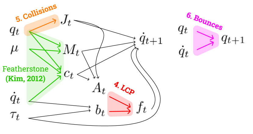
Figure 2: Data flow during a forward timestep computation. Each arrow represents a dependency. We can use the adjoint method to assemble Jacobians relating $q_{t}$, $\dot{\boldsymbol{q}}_{t}$, $\boldsymbol{\mu}$ and $\tau$ with $\dot{\boldsymbol{q}}_{t+1}$.[Karen: There should be arrows between (M,b), (c,b), and (J,b), and no arrow between (c,A). Also, if we define $\mu$ to be both mass and link dimensions, $J$ will depend on $\mu$, too, because Jabocian depends on the link dimensions. ][JS: Q: Do we have $\mu$ here for the case that the mass properties are regarded as variable in RL for example?]

The main task in developing a differentiable physics engine is to solve for the gradient of next velocity $\dot{\boldsymbol{q}}_{t+1}$ with respect to the input to the current time step, namely $\boldsymbol{q}_{t},\dot{\boldsymbol{q}}_{t},\bm{\tau}_{t}$, and $\bm{\mu}$. The data flow is shown in Figure 2. For brevity we refer to the ouput of a function for a given timestep by the same name as the function with a subscript $t$ (e.g. $\bm{J}_{t}=\bm{J}(\boldsymbol{q}_{t})$). The velocity at the next step can be simplified to

$$\dot{\bm{q}}_{t+1}=\dot{\bm{q}}_{t}+\bm{M}_{t}^{-1}\bm{z}_{t},$$

where $\boldsymbol{z}_{t}\equiv-\Delta t(\bm{c}_{t}-\bm{\tau}_{t})+\bm{J}_{t}^{T}\bm{f}_{t}$. The gradients we need to compute at each time step are written as:

$$\frac{\partial\dot{\bm{q}}_{t+1}}{\partial\bm{q}_{t}} =\frac{\partial\bm{M}_{t}^{-1}\boldsymbol{z}_{t}}{\partial\boldsymbol{q}_{t}}+\bm{M}_{t}^{-1}(-\Delta t\frac{\partial\bm{c}_{t}}{\partial\boldsymbol{q}_{t}}+\frac{\partial\bm{J}_{t}^{T}}{\partial\boldsymbol{q}_{t}}\bm{f}_{t}$$

$$+\boldsymbol{J}_{t}^{T}\frac{\partial{\boldsymbol{f}_{t}}}{\partial\boldsymbol{q}_{t}})$$ (7)

$$\frac{\partial\dot{\bm{q}}_{t+1}}{\partial\dot{\bm{q}}_{t}} =\bm{I}+\boldsymbol{M}_{t}^{-1}(-\Delta t\frac{\partial\boldsymbol{c}_{t}}{\partial\dot{\boldsymbol{q}}_{t}}+\boldsymbol{J}_{t}^{T}\frac{\partial\boldsymbol{f}_{t}}{\partial\dot{\boldsymbol{q}}_{t}})$$ (8)

$$\frac{\partial\dot{\bm{q}}_{t+1}}{\partial\bm{\tau}_{t}} =\boldsymbol{M}_{t}^{-1}(\Delta t\bm{I}+\boldsymbol{J}_{t}^{T}\frac{\partial\boldsymbol{f}_{t}}{\partial\boldsymbol{\tau}_{t}})$$ (9)

$$\frac{\partial\dot{\bm{q}}_{t+1}}{\partial\bm{\mu}} =\frac{\partial\boldsymbol{M}_{t}^{-1}\boldsymbol{z}_{t}}{\partial\boldsymbol{\mu}}+\boldsymbol{M}_{t}^{-1}(-\Delta t\frac{\partial\boldsymbol{c}_{t}}{\partial\boldsymbol{\mu}}+\boldsymbol{J}_{t}^{T}\frac{\partial\boldsymbol{f}_{t}}{\partial\boldsymbol{\mu}})$$ (10)

We will tackle several of the trickiest intermediate Jacobians in sections that follow. In Section 4 we will introduce a novel sparse analytical method to compute the gradients of contact force $\boldsymbol{f}_{t}$ with respect to $\boldsymbol{q}_{t},\dot{\boldsymbol{q}}_{t},\bm{\tau}_{t},\bm{\mu}$. Section 5 will discuss $\frac{\partial\boldsymbol{J}_{t}}{\partial\boldsymbol{q}_{t}}$—how collision geometry changes with respect to changes in position? In Section 6 we will tackle $\frac{\partial\boldsymbol{q}_{t+1}}{\partial\boldsymbol{q}_{t}}$ and $\frac{\partial\boldsymbol{q}_{t+1}}{\partial\dot{\boldsymbol{q}}_{t}}$, which is not as simple as it may at first appear, because naively taking gradients through a discrete time physics engine yields incorrect results when elastic collisions take place. Finally, Section LABEL:sec:featherstone will give a way to apply the derivations from (kim2012lie) to analytically find $\frac{\partial\boldsymbol{M}_{t}}{\partial\boldsymbol{q}_{t}}$, $\frac{\partial\boldsymbol{M}_{t}}{\partial\bm{\mu}}$, $\frac{\partial\boldsymbol{c}_{t}}{\partial\boldsymbol{q}_{t}}$, $\frac{\partial\boldsymbol{c}_{t}}{\partial\bm{\mu}}$, and $\frac{\partial\boldsymbol{c}_{t}}{\partial\dot{\boldsymbol{q}}_{t}}$.

4 Differentiating the LCP

This section introduces a method to analytically compute $\frac{\partial\boldsymbol{f}}{\partial\boldsymbol{A}}$ and $\frac{\partial\boldsymbol{f}}{\partial\boldsymbol{b}}$. It turns out that it is possible to get unambiguous gradients through an LCP in the vast majority of practical scenarios, without recasting it as a QP. To see this, let us consider a hypothetical LCP problem parameterized by $\boldsymbol{A},\boldsymbol{b}$ with a solution $\boldsymbol{f}^{*}$ found previously: $f_{LCP}(\bm{A},\bm{b})=\bm{f}^{*}$.

For brevity, we only include the discussion on normal contact impulses in this section and leave the friction impulses in Appendix X. Therefore, each element in $\boldsymbol{f}^{*}\geq\boldsymbol{0}$ indicates the normal impulse of a point contact. By complementarity, we know that if some element $f^{*}_{i}>0$, then $v_{i}=(\boldsymbol{A}\boldsymbol{f}^{*}+\boldsymbol{b})_{i}=0$. Intuitively, the relative velocity at contact point $i$ must be 0 if there is any non-zero impulse being exerted at contact point $i$. Let us call such contact points “Clamping” because the LCP is changing the impulse $f_{i}>0$ to keep the relative velocity $v_{i}=0$. Let us define the set $\mathcal{C}$ to be all indices that are clamping. Symmetrically, if $f_{j}=0$ for some index $j$, then the relative velocity $v_{j}=(\boldsymbol{A}\boldsymbol{f}^{*}+\boldsymbol{b})_{j}\geq 0$ is free to vary without the LCP needing to adjust $f_{j}$ to compensate. We call such contact points “Separating” and define the set $\mathcal{S}$ to be all indices that are separating. Let us call indices $j$ where $f_{j}=0$ and $v_{j}=0$ “Tied.” Define the set $\mathcal{T}$ to be all indices that are tied.

If no contact points are tied ($\mathcal{T}=\emptyset$), the LCP is strictly differentiable and the gradients can be analytically computed. When some contact points are tied ($\mathcal{T}\neq\emptyset$), the LCP has a couple of valid subgradients and it is possible to follow any in an optimization. The tied case is analogous to the non-differentiable points in a QP where an inequality constraint is active while the corresponding dual variable is also zero. In such case, computing gradients via taking differentials of the KKT conditions will result in a low-rank linear system and thus non-unique gradients (amos2017optnet).

4.1 Strictly differentiable cases

Consider the case where $\mathcal{T}=\emptyset$. We shuffle the indices of $\boldsymbol{f}^{*}$, $\boldsymbol{v}$, $\boldsymbol{A}$ and $\boldsymbol{b}$ to group together members of $\mathcal{C}$ and $\mathcal{S}$. The LCP becomes:

$$\begin{matrix}[l]\text{find}&&\boldsymbol{f}^{*}_{\mathcal{C}},\boldsymbol{f}^{*}_{\mathcal{S}},\boldsymbol{v}_{\mathcal{C}},\boldsymbol{v}_{\mathcal{S}}\\ \text{such that}&&\begin{bmatrix}\boldsymbol{v}_{\mathcal{C}}\\ \boldsymbol{v}_{\mathcal{S}}\end{bmatrix}=\begin{bmatrix}\boldsymbol{A}_{\mathcal{CC}}&&\boldsymbol{A}_{\mathcal{CS}}\\ \boldsymbol{A}_{\mathcal{SC}}&&\boldsymbol{A}_{\mathcal{SS}}\\ \end{bmatrix}\begin{bmatrix}\boldsymbol{f}^{*}_{\mathcal{C}}\\ \boldsymbol{f}^{*}_{\mathcal{S}}\end{bmatrix}+\begin{bmatrix}\boldsymbol{b}_{\mathcal{C}}\\ \boldsymbol{b}_{\mathcal{S}}\end{bmatrix}\\ &&\boldsymbol{f}^{*}_{\mathcal{C}}\geq\boldsymbol{0},\;\boldsymbol{f}^{*}_{\mathcal{S}}\geq\boldsymbol{0},\;\boldsymbol{v}_{\mathcal{C}}\geq\boldsymbol{0},\;\boldsymbol{v}_{\mathcal{S}}\geq\boldsymbol{0}\\ &&\boldsymbol{f}_{\mathcal{C}}^{*T}\boldsymbol{v}_{\mathcal{C}}=0,\;\boldsymbol{f}_{\mathcal{S}}^{*T}\boldsymbol{v}_{\mathcal{S}}=0\\ \end{matrix}$$ (11)

Since we know the classification of each contact that forms the valid solution $\boldsymbol{f}^{*}$, we rewrite the LCP as follows:

$$\begin{matrix}[l]\text{find}&&\boldsymbol{f}^{*}_{\mathcal{C}},\boldsymbol{f}^{*}_{\mathcal{S}},\boldsymbol{v}_{\mathcal{C}},\boldsymbol{v}_{\mathcal{S}}\\ \text{such that}&&\begin{bmatrix}\boldsymbol{v}_{\mathcal{C}}\\ \boldsymbol{v}_{\mathcal{S}}\end{bmatrix}=\begin{bmatrix}\boldsymbol{A}_{\mathcal{CC}}&&\boldsymbol{A}_{\mathcal{CS}}\\ \boldsymbol{A}_{\mathcal{SC}}&&\boldsymbol{A}_{\mathcal{SS}}\\ \end{bmatrix}\begin{bmatrix}\boldsymbol{f}^{*}_{\mathcal{C}}\\ \boldsymbol{f}^{*}_{\mathcal{S}}\end{bmatrix}+\begin{bmatrix}\boldsymbol{b}_{\mathcal{C}}\\ \boldsymbol{b}_{\mathcal{S}}\end{bmatrix}\\ &&\boldsymbol{f}^{*}_{\mathcal{C}}>\boldsymbol{0},\;\boldsymbol{f}^{*}_{\mathcal{S}}=\boldsymbol{0},\;\boldsymbol{v}_{\mathcal{C}}=\boldsymbol{0},\;\boldsymbol{v}_{\mathcal{S}}>\boldsymbol{0}\end{matrix}$$

From here we can see how the valid solution $\boldsymbol{f}^{*}$ changes under infinitesimal perturbations $\bm{\epsilon}$ to $\boldsymbol{A}$ and $\boldsymbol{b}$. Since $\boldsymbol{f}^{*}_{\mathcal{S}}=\boldsymbol{0}$ and $\boldsymbol{v}_{\mathcal{C}}=\boldsymbol{0}$, the LCP can be reduced to three conditions on $\boldsymbol{f}^{*}_{\mathcal{C}}$:

$$\boldsymbol{0}=\boldsymbol{A}_{\mathcal{CC}}\boldsymbol{f}^{*}_{\mathcal{C}}+\boldsymbol{b}_{\mathcal{C}}$$ (12)

$$\boldsymbol{f}^{*}_{\mathcal{C}}>\boldsymbol{0}$$ (13)

$$\boldsymbol{A}_{\mathcal{SC}}\boldsymbol{f}^{*}_{\mathcal{C}}+\boldsymbol{b}_{\mathcal{S}}>\boldsymbol{0}$$ (14)

We will show that these conditions will always be possible to satisfy under small enough perturbations $\bm{\epsilon}$ in the neighborhood of a valid solution. Let us first consider tiny perturbations to $\boldsymbol{b}_{\mathcal{S}}$ and $\boldsymbol{A}_{\mathcal{SC}}$. If the perturbations are small enough, then Equation 14 will still be satisfied with our original $\boldsymbol{f}_{\mathcal{C}}^{*}$, because we know Equation 14 already holds strictly such that there is some non-zero room to decrease any element of $\boldsymbol{A}_{\mathcal{SC}}\boldsymbol{f}^{*}_{\mathcal{C}}+\boldsymbol{b}_{\mathcal{S}}$ without violating Equation 14. Therefor,

$$\frac{\partial\boldsymbol{f}_{\mathcal{C}}^{*}}{\partial\boldsymbol{b}_{\mathcal{S}}}=\boldsymbol{0}\text{\;\;and\;\;}\frac{\partial\boldsymbol{f}_{\mathcal{C}}^{*}}{\partial\boldsymbol{A}_{\mathcal{SC}}}=\boldsymbol{0}$$

Next let us consider an infinitesimal perturbation $\bm{\epsilon}$ to $\boldsymbol{b}_{\mathcal{C}}$ and the necessary change on the clamping force $\Delta\boldsymbol{f}_{\mathcal{C}}^{*}$ to satisfy Equation 12:

$$\boldsymbol{0}=\boldsymbol{A}_{\mathcal{CC}}(\boldsymbol{f}^{*}_{\mathcal{C}}+\Delta\boldsymbol{f}^{*}_{\mathcal{C}})+\boldsymbol{b}_{\mathcal{C}}+\bm{\epsilon}.$$ (15)

Setting $\boldsymbol{A}_{\mathcal{CC}}\boldsymbol{f}^{*}_{\mathcal{C}}+\boldsymbol{b}_{\mathcal{C}}=\boldsymbol{0}$ and assuming $\boldsymbol{A}_{\mathcal{CC}}$ is invertible, the change of the clamping force is given as

$$\Delta\boldsymbol{f}^{*}_{\mathcal{C}}=-\boldsymbol{A}_{\mathcal{CC}}^{-1}\bm{\epsilon}.$$

Since $\boldsymbol{f}^{*}_{\mathcal{C}}$ is strictly greater than $\boldsymbol{0}$, it is always possible to choose an $\bm{\epsilon}$ small enough to make $\boldsymbol{f}^{*}_{\mathcal{C}}-\boldsymbol{A}_{\mathcal{CC}}^{-1}\bm{\epsilon}>0$ and $\boldsymbol{A}_{\mathcal{SC}}(\boldsymbol{f}^{*}_{\mathcal{C}}+\Delta\boldsymbol{f}^{*}_{\mathcal{C}})+\boldsymbol{b}_{\mathcal{S}}>0$ remain true. Therefor,

$$\frac{\partial\boldsymbol{f}_{\mathcal{C}}^{*}}{\partial\boldsymbol{b}_{\mathcal{C}}}=-\boldsymbol{A}_{\mathcal{CC}}^{-1}$$

Note that $\boldsymbol{A}_{\mathcal{CC}}$ is not always invertible because $\boldsymbol{A}$ is positive semidefinite. We will discuss the case when $\boldsymbol{A}_{\mathcal{CC}}$ is not full rank in Section 4.3 along with the proposed method to stabilize the gradients when there exists multiple LCP solutions in Appendix X.

Last up is computing gradients with respect to $\boldsymbol{A}_{\mathcal{CC}}$. In practice, changes to $\boldsymbol{A}_{\mathcal{CC}}$ only happen because we are differentiating with respect to parameters $\boldsymbol{q}$ or $\bm{\mu}$, which also changes $\boldsymbol{b}_{\mathcal{C}}$. As such, we introduce a new scalar variable, $x$, which could represent any arbitrary scalar quantity that effects both $\boldsymbol{A}$ and $\boldsymbol{b}$. Equation 12 can be rewritten as:

$$\boldsymbol{f}^{*}_{\mathcal{C}}=-\boldsymbol{A}_{\mathcal{CC}}(x)^{-1}\boldsymbol{b}_{\mathcal{C}}(x)$$

Because $\boldsymbol{A}_{\mathcal{CC}}(x)$ and $\boldsymbol{b}_{\mathcal{C}}(x)$ are continuous, and the original solution is valid, any sufficiently small perturbation to $x$ will not reduce $\boldsymbol{f}^{*}_{\mathcal{C}}$ below 0 or violating Equation 14. The Jacobian with respect to $x$ can be expressed as:

$$\frac{\partial\boldsymbol{f}^{*}_{\mathcal{C}}}{\partial x}=\boldsymbol{A}_{\mathcal{CC}}(x)^{-1}\frac{\partial\boldsymbol{A}_{\mathcal{CC}}(x)}{\partial x}\boldsymbol{A}_{\mathcal{CC}}(x)^{-1}\boldsymbol{b}_{\mathcal{C}}(x)$$

$$+\boldsymbol{A}_{\mathcal{CC}}(x)^{-1}\frac{\partial\boldsymbol{b}_{\mathcal{C}}(x)}{\partial x}$$ (16)

Section LABEL:sec:featherstone will describe $\frac{\partial\boldsymbol{A}_{\mathcal{CC}}}{\partial x}$ and $\frac{\partial\boldsymbol{b}_{\mathcal{C}}}{\partial x}$ for any specific $x$.

Remark: Previous methods (de2018end; cloth; qiao) cast a LCP to a QP and solved for a linear system of size $n+m$ derived from taking differentials of the KKT conditions of the QP, where $n$ is the dimension of the state variable and $m$ is the number of contact constraints. Our method also solves for linear systems to obtain $\bm{A}_{\mathcal{CC}}^{-1}$, but the size of $\bm{A}_{\mathcal{CC}}$ is less than $m$ due to the sparsity of the original matrix $\bm{A}$.

4.2 Subdifferentiable case

Now let us consider when $\mathcal{T}\neq\emptyset$. Replacing the LCP constraints with linear constraints will no longer work because any perturbation will immediately change the state of the contact and the change also depends on the direction of perturbation. Including the class of ”tied” contact points to Equation 11, we need to satisfy an additional linear system,

$$\bm{v}_{\mathcal{T}} =\bm{A}_{\mathcal{TT}}\bm{f}_{\mathcal{T}}^{*}+\bm{A}_{\mathcal{TC}}\bm{f}_{\mathcal{C}}^{*}+\bm{A}_{\mathcal{TS}}\bm{f}_{\mathcal{S}}^{*}+\bm{b}_{\mathcal{T}}$$

$$=\bm{A}_{\mathcal{TT}}\bm{f}_{\mathcal{T}}^{*}+\tilde{\bm{b}}_{\mathcal{T}},$$ (17)

where $\tilde{\bm{b}}_{\mathcal{T}}=\bm{A}_{\mathcal{TC}}\bm{f}_{\mathcal{C}}^{*}+\bm{b}_{\mathcal{T}}$ and $\bm{v}_{\mathcal{T}}$ and $\bm{f}_{\mathcal{T}}^{*}$ are both zero at the solution. Let $i\in\mathcal{T}$ be the index of a tied contact point. Consider perturbing the $i^{th}$ element of $\tilde{\boldsymbol{b}}_{\mathcal{T}}$ by $\epsilon$. If $\epsilon>0$, $\bm{A}_{\mathcal{TT}}\bm{f}_{\mathcal{T}}^{*}$ cannot become negative to balance Equation 4.2 because $\bm{A}_{\mathcal{TT}}$ is positive semidefinite and $\bm{f}_{\mathcal{T}}^{*}$ must be nonnegative. Therefore, $v_{\mathcal{T}i}$ must become positive, resulting contact point $i$ being separated and $f_{\mathcal{T}i}^{*}$ remaining zero. If $\epsilon<0$, then $i$ is immediately bumped into the “clamping” set $\mathcal{C}$ because $v_{\mathcal{T}i}$ cannot be negative. Therefore, $f^{*}_{\mathcal{T}i}$ must become positive to balance Equation 4.2. The gradients for the clamping and separating cases are both valid subgraidents for a tied contact point. In an optimization, we can choose either of the two subgradients at random without impacting the convergence (boyd2003subgradient). In practice, encountering elements in $\mathcal{T}$ is quite rare for practical numerical reasons.

4.3 When $\boldsymbol{A}_{\mathcal{CC}}$ is not full rank

When $\boldsymbol{A}_{\mathcal{CC}}$ is not full rank, the solution to $f_{LCP}(\boldsymbol{A},\boldsymbol{b})=\boldsymbol{f}^{*}$ is no longer unique. Nevertheless, once a solution is computed using any algorithm and the clamping set $\mathcal{C}$ is found, the gradient of clamping forces can be written as:

$$\frac{\partial\boldsymbol{f}^{*}_{\mathcal{C}}}{\partial x}=\boldsymbol{A}_{\mathcal{CC}}^{-1}\frac{\partial\boldsymbol{A}_{\mathcal{CC}}}{\partial x}\boldsymbol{A}_{\mathcal{CC}}^{-1}\boldsymbol{b}_{\mathcal{C}}+\boldsymbol{A}_{\mathcal{CC}}^{-1}\frac{\partial\boldsymbol{b}_{\mathcal{C}}}{\partial x}$$

$$+(\boldsymbol{I}-\boldsymbol{A}^{+}_{\mathcal{CC}}\boldsymbol{A}_{\mathcal{CC}})\big{(}\frac{\partial\boldsymbol{A}_{\mathcal{CC}}^{T}}{\partial x}\big{)}\boldsymbol{A}_{\mathcal{CC}}^{+T}\boldsymbol{A}_{\mathcal{CC}}^{+},$$ (18)

where $\boldsymbol{A}_{\mathcal{CC}}^{+}$ is the pseudo inverse matrix of the low-rank $\boldsymbol{A}$. For numerical stability, we can solve a series of linear systems instead of explicitly evaluating $\boldsymbol{A}_{\mathcal{CC}}(x)^{+}$.

To have smoother gradients across timesteps, the forward solving of LCP needs to have deterministic and stable behavior when faced with multiple valid solutions. We propose a simple and efficient LCP stabilization method detailed in Appendix X.

4.4 Escaping saddle-points during learning

The above analysis gives us a foundation to understand one reason why ordinary gradient descent is so sensitive to initialization for physical problems involving contact. In this section, we explain the saddle points that arise as the result of “Clamping” indices, and propose a method for escaping these saddle points.

To fully state the contact $\text{LCP}(\boldsymbol{A},\boldsymbol{b})=\boldsymbol{v}$, we have:

$$\begin{matrix}[l]\text{find}&&\boldsymbol{f},\boldsymbol{v}\\ \text{such that}&&\boldsymbol{A}\boldsymbol{f}-\boldsymbol{b}=\boldsymbol{v}\\ &&\boldsymbol{f}\geq 0\\ &&\boldsymbol{v}\geq 0\\ &&\boldsymbol{f}^{T}\boldsymbol{v}=0\end{matrix}$$

Suppose we have some desired result velocity, $\boldsymbol{v}^{*}$. Let’s pose an optimization problem: we’d like to find an appropriate $\boldsymbol{b}$ (while holding $\boldsymbol{A}$ fixed) to minimize a loss function $\ell(\boldsymbol{v})=||\boldsymbol{v}-\boldsymbol{v}^{*}||$. We’ll use a gradient descent method. Each iteration of this algorithm will backpropagate $\frac{\partial\boldsymbol{v}}{\partial\ell}$ to $\frac{\partial\boldsymbol{b}}{\partial\ell}$, through the LCP solution, before updating $\boldsymbol{b}$ and re-solving the LCP. When put in context of our whole engine, this exact operation occurs (holding $\boldsymbol{A}$ fixed, finding $\frac{\partial\boldsymbol{b}}{\partial\ell}$) when backpropagating our gradient wrt loss from next timestep’s velocity to gradient wrt loss from this timestep’s velocity or force vectors.

To see the problem that can arise, let’s consider a very simple one dimensional physical problem involving an LCP. Consider a 2D circle attached to a linear actuator that can produce force along the y axis. The circle is resting on the ground.

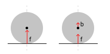
Figure 3: Increasing force from the linear actuator ($\boldsymbol{b}$) is met by an equal and opposite decrease in ground reaction force ($\boldsymbol{f}$), resulting in 0 change in velocity. In other words, $\frac{\partial\boldsymbol{v}}{\partial\boldsymbol{b}}=0$

In this example, the linear actuator’s power is linearly related to $\boldsymbol{b}$, and the resulting relative velocity of the circle and the ground at the next timestep is $\boldsymbol{v}$.

The problem arises if we want to use gradient descent to find a $\boldsymbol{b}$ vector that will cause the circle to leave the ground, which would mean $\boldsymbol{v}>1$. If we initialize a starting $\boldsymbol{b}<mg$, we will never find a solution where $\boldsymbol{b}>mg$.

It’s intuitively obvious that the way to make the circle leave the ground is to provide enough force in the linear actuator to overcome gravity. However, our gradient descent algorithm will never find this solution, unless it is initialized into it.

This is because of the behavior of “Clamping” indices. In effect, an index $i$ being “Clamping” means that the complimentarity constraint will prevent an change in $\boldsymbol{b}_{i}$ from having any impact whatsoever on $\boldsymbol{v}_{i}$, because $\boldsymbol{f}$ will vary to always ensure that $\boldsymbol{v}_{i}=0$.

In our example, because the circle is resting on the ground, it has a non-zero normal force. That means that the circle-ground contact is “Clamping.” Because it’s clamping, any tiny perturbation $\epsilon$ in the amount of linear actuator force $\boldsymbol{b}$ will be met with an exactly offsetting tiny perturbation $\epsilon$ in normal force $\boldsymbol{A}\boldsymbol{f}$, and the resulting change in $\boldsymbol{v}$ will be 0. That, in turn, means that $\frac{\partial\boldsymbol{v}}{\partial\boldsymbol{b}}=0$. And that means that no matter what gradient of loss $\frac{\partial\boldsymbol{v}}{\partial\ell}$ we try to backpropagate through our LCP, we will always get $\frac{\partial\boldsymbol{b}}{\partial\ell}=0$. That means learning will be impossible, because we have a 0 gradient and we’re not at a local optimum. We’re trapped in a saddle point.

To overcome this problem, we need to consider how we could set $\frac{\partial\boldsymbol{b}}{\partial\ell}$ to be the “best search direction” for $\boldsymbol{b}$ in order to move $\boldsymbol{v}$ along $\frac{\partial\boldsymbol{v}}{\partial\ell}$. Our problem really boils down to the myopia of the real gradient: it considers only an infinitely small region around our current point, perturbations $\epsilon$ around $\boldsymbol{b}$. Unfortunately $\epsilon$ is too small to see the discontinuity where $\boldsymbol{b}$ becomes large enough to overcome gravity, and suddenly $\frac{\partial\boldsymbol{v}}{\partial\boldsymbol{b}}=1$. Instead, in its local neighborhood, $\frac{\partial\boldsymbol{v}}{\partial\boldsymbol{b}}=0$, because normal force is fighting any changes to $\boldsymbol{b}$.

We propose to project to the nearest edge of our saddle point in the direction of $\frac{\partial\boldsymbol{v}}{\partial\ell}$, and get the (non-zero) gradient of $\frac{\partial\boldsymbol{b}}{\partial\ell}$ from there, if one exists. In practice, this is quite straightforward, since we have one non-linearity per variable, and they are all at 0, and independent for each index. To find an intelligent search direction, for any given index $i$, if we have $\frac{\partial\boldsymbol{v}}{\partial\ell}_{i}>0$ (which means we want to increase $\boldsymbol{b}_{i}$), and index $i$ is currently “Clamping” (which would block gradient flow to $\boldsymbol{b}_{i}$) then we arbitrarily declare index $i$ to be “Separating” for the duration of this backpropagation, and proceed otherwise normally. This has the effect of projecting index $\boldsymbol{b}_{i}$ “forward” to a point where it’s accumulated enough force to cause $\boldsymbol{f}_{i}$ to sit at 0, which allows breaking the contact. Said another way, this prevents $\boldsymbol{f}_{i}$ from “blocking” the gradients flowing backwards from $\frac{\partial\boldsymbol{v}_{i}}{\partial\ell}$ to $\frac{\partial\boldsymbol{b}_{i}}{\partial\ell}$. This gives the optimizer a chance to see what happens if it moves $\boldsymbol{b}_{i}$ upwards far enough.

For a clamping index $i$ where we have $\frac{\partial\boldsymbol{v}}{\partial\ell}_{i}\leq 0$, we leave it in “Clamping.” This corresponds to an infinite projection downwards in $\boldsymbol{b}_{i}$, which never encounters a discontinuity. Said another way, no matter how hard you push down on the floor (at least in an idealized rigid body simulation), pushing harder is never going to help you reach 0 normal force.

Updated version:

When you have a contact between two objects, there’s really two “strategies” that are available for force generation. The optimizer can either attempt to exploit the normal force between the objects to achieve its desired objective, or it can attempt to directly control the objects separately to achieve its desired objective.

When we’re taking gradients, we need to decide in advance what strategies to use for which contact points. This is important: The optimizer can’t simultaneously explore both strategies (normal force vs. separate control) for the same contact point! If we choose to try to exploit normal force, we put constraints on the Jacobians that mean that we’ll get 0 gradients for losses trying to encourage us to separately control the objects. Similarly, if we choose to try to control the objects separately, we remove constraints on the Jacobians that mean that we’ll get 0 gradients for losses trying to encourage us to use the normal forces.

When we label a contact as clamping, we force the optimizer to only explore the “normal force strategy” for getting results. When we’ve clamped two objects together, the gradients make it seem as though they’re welded at that point, and will move as a unit with respect to changes in velocity and forces. In our Jacobians we enforce the constraint that the contact velocity is 0 at that index $i$ ($v_{i}=0$), by varying contact force to achieve that. From the perspective of the Jacobians, any force or impulse on either object, in any direction, will apply to both objects, because contact velocity must remain 0. This is technically correct, for small enough perturbations $\epsilon$ around the existing conditions that led to this contact being classified as clamping. But it does mean that the optimizer will be blinded to any loss that would require forces or velocity changes that lead the contact point separate (where $v_{i}\neq 0$).

Symmetrically, when we label a contact as separating, we don’t apply any constraints to the relative velocity of the two objects at the contact point. From the perspective of the Jacobians, this means the contact may as well not exist: the objects can have velocities or forces moving them apart, but they can also have velocities or forces moving them together without the normal force changing.

Forcing the Jacobians to encode a strategy for each contact point is technically correct (see the LCP proofs in the previous section). However, it’s obvious that in some scenarios this myopia encoded in our naive gradients can lead to bad outcomes during optimization.

[Keenon: TODO: copy the ball on floor example]

Figure 4: Increasing force from the linear actuator ($\boldsymbol{b}$) is met by an equal and opposite decrease in ground reaction force ($\boldsymbol{f}$), resulting in 0 change in velocity. In other words, $\frac{\partial\boldsymbol{v}}{\partial\boldsymbol{b}}=0$

In the case of a ball resting on the floor, we’d like the optimizer to explore separate control instead of only using the normal force. If the optimizer tries to use normal force on a ball resting on the floor, it’ll never make any progress, because it can’t use the normal force to make the ball leave the ground. We could fix this specific problem by classifying the contact point between the ball and the ground as “separating”, regardless of it’s real classification.

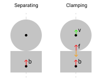
Figure 5: Increasing force from the linear actuator on the block ($\boldsymbol{b}$) is met by an increase in normal force ($\boldsymbol{f}$) if this contact is classified as “Clamping”. If it’s classified as “Separating” the gradient can’t predict any force transmitted from the block to the ball, resulting in 0 change in velocity when we increase force on the block. In other words, $\frac{\partial\boldsymbol{v}}{\partial\boldsymbol{b}}=0$

There are other cases where we want to use the normal force strategy. For example, imagine that same ball is uncontrolled, and is resting on a platform that is attached to a linear actuator. We still want to move the ball to the same place. Now we absolutely want the optimizer to use the normal force strategy, because direct control of the ball will result in 0 gradients, since it’s uncontrolled.

Is there a way to know which strategy we want to use in advance? In general, the answer seems to be no, but we can certainly do better than naive gradients. Naive gradients stick with whatever strategy they were initialized into, and don’t explore to break out of resulting saddle points. We propose a heuristic to explore somewhat more broadly at a constant additional cost, which fixes the issues in the simple examples we’ve highlighted above. We leave it to future work to explore more possible heuristics, and their effect on more complex optimizations.

The failure cases we’ve highlighted above can be detected because the gradients $\frac{\partial\ell}{\partial\dot{q}_{t}}$ and $\frac{\partial\ell}{\partial\tau_{t}}$ are 0, which means we’ve hit a saddle point (at least as long as we stick to this strategy). Inspired by this fact, let’s go with the set of contact strategies for our contact points that reduces loss the fastest. So let’s simply pick a strategy where the norms $||\frac{\partial\ell}{\partial\dot{q}_{t}}||_{2}^{2}+||\frac{\partial\ell}{\partial\tau_{t}}||_{2}^{2}$ are the largest.

In the worst case, exploring all possible combinations of strategies for all possible contact points is $\mathcal{O}(2^{n})$, which is disastrous as $n$ grows.

There are lots of possible ways to pick a subset of the $2^{n}$ strategies to explore. We propose only checking two strategies:

1. First, check the “correct” strategy, given to us by the real Jacobians.

2. Second, we compute $\frac{\partial\ell}{\partial f}$, and use the elements of $\frac{\partial\ell}{\partial f}$ to compute the “Clamping” and “Separating” sets as follows (ignoring the LCP). Take any indices $i$ that are trying to reduce the normal force at that contact $\frac{\partial\ell}{\partial f_{i}}<0$, which implies the optimizer is feebly trying to separate the objects, and put those indices into “Separating”. Take any indices $i$ where $\frac{\partial\ell}{\partial f_{i}}>0$, which implies the optimizer is trying to exploit the normal force between objects, and put them into “Clamping”.

If our “loss driven contact strategy” just described produces a larger magnitude for our loss gradients, then keep it. Otherwise, ignore it and stick with the original gradients.

Computing $\frac{\partial\ell}{\partial f_{i}}$ from $\frac{\partial\ell}{\partial\dot{q}_{t+1}}$: we need to get the Jacobian $\frac{\partial\dot{q}_{t+1}}{\partial f}$. This is straightforward:

$$\frac{\partial\dot{q}_{t+1}}{\partial f}=M^{-1}J^{T}$$

Then we can use the ordinary transpose rule for backprop:

$$\frac{\partial\ell}{\partial f}=\frac{\partial\dot{q}_{t+1}}{\partial f}^{T}\frac{\partial\ell}{\partial\dot{q}_{t+1}}=JM^{-1}\frac{\partial\ell}{\partial\dot{q}_{t+1}}$$

5 Gradients through collision geometry

This section addresses efficient computation of $\frac{\partial\boldsymbol{J}_{t}^{T}\boldsymbol{f}}{\partial\boldsymbol{q}_{t}}$, the relationship between position and joint impulse. In theory, we could utilize auto-diff libraries for the derivative computation. In practice, however, passing every gradient through a long kinematic chain of transformations is inefficient for complex articulated rigid body systems. In contrast, computing the gradients symbolically shortcuts much computation by operating directly in the world coordinate frame.

Let $\mathcal{A}_{i}\in se(3)$ be the screw axis for the $i$’th DOF, expressed in the world frame. Let the $k$’th contact point give an impulse $\mathcal{F}_{k}\in dse(3)$, also expressed in the world frame. The total joint impulse caused by contact impulses for the $i$’th joint is given by:

$$(\boldsymbol{J}_{t}^{T}\boldsymbol{f})_{i}=\sum_{k}\mathcal{A}_{i}^{T}\mathcal{F}_{k}=\mathcal{A}_{i}^{T}\sum_{k}\mathcal{F}_{k}.$$ (19)

Taking the derivative of Equation 19 gives

$$\frac{\partial(\boldsymbol{J}_{t}^{T}\boldsymbol{f})_{i}}{\partial\boldsymbol{q}_{t}}=\frac{\partial\mathcal{A}_{i}}{\partial\boldsymbol{q}_{t}}^{T}\sum_{k}\mathcal{F}_{k}+\mathcal{A}_{i}^{T}\sum_{k}\frac{\partial\mathcal{F}_{k}}{\partial\boldsymbol{q}_{t}}.$$ (20)

Evaluating the Jacobian $\frac{\partial\mathcal{A}_{i}}{\partial\boldsymbol{q}_{t}}$ is straightforward, but computing $\frac{\partial\mathcal{F}_{k}}{\partial q_{t}}$ requires understanding how the contact normal $\boldsymbol{n}_{k}\in\mathcal{R}^{3}$ and contact position $\boldsymbol{p}_{k}\in\mathcal{R}^{3}$ change with changes in $\boldsymbol{q}_{t}$.

To compute gradients through each contact point and normal with respect to $\boldsymbol{q}_{t}$, we need provide specialized routines for each type of collision geometry, including collisions between spheres, capsules, boxes, and arbitrary convex meshes. For illustration purposes, we only focus on mesh-mesh collisions, and refer readers to the appendix for handling of other combinations of meshes and/or primitive shapes. Mesh-mesh collisions only have two types of contacts: vertex-face and edge-edge collisions. The other cases (vertex-edge, vertex-vertex, edge-face, face-face) are degenerate and easily mapped into vertex-face and edge-edge collisions.

5.1 Vertex-face collisions

During the forward simulation, the collision detector places a collision at the point of the vertex, with a normal dictated by the face under collision. The body providing the vertex can only influence the collision location $\boldsymbol{p}$, and the body providing the face can only influence the collision normal $\boldsymbol{n}$.

TODO(keenon): illustrations

5.2 Edge-edge collisions

During the forward simulation, the collision detector places a collision at the nearest point between the two edges, with a normal dictated by the cross product of the two edges. [Karen: So does that mean changing $\boldsymbol{q}$ of Object A can affect the contact normal and the contact location along the other edge from Object B?] [Keenon: Indeed it does, unfortunately. These Jacobians need to be constructed globally for that reason. As we extended to other types of primitive shapes like spheres and capsules, this sort of entanglement turned out to be more common than not.]

With that, it’s possible to efficiently compute $\frac{\partial J_{t}^{T}f}{\partial q_{t}}$. [Karen: Need to talk more on how $\frac{\partial\boldsymbol{p}}{\partial\boldsymbol{q}}$ and $\frac{\partial\boldsymbol{n}}{\partial\boldsymbol{q}}$ are related to $\frac{\partial\mathcal{F}_{k}}{\partial\boldsymbol{q}_{t}}$.]

6 Gradients through elastic contacts

DiffTaichi (difftaichi) pointed out an interesting problem that arises from discretization of time in simulating elastic bouncing phenomenon between two objects. Suppose we have a trivial system with one degree of freedom: a bouncing ball confined to a single axis of motion. Let the ball’s height be given by $q$ and is perfectly elastic (coefficient or restitution, $e=1$). Consider the time step when the height of the ball is within some numerical tolerance from the ground, $q_{t}<\epsilon$. The velocity at the next time step will be $\dot{q}_{t+1}=-\dot{q}_{t}$. A problem arises when computing $\frac{\partial q_{t+1}}{\partial q_{t}}$ at this time step. We would intuitively expect that as we lower $q_{t}$, we cause the ball to hit the ground sooner and have more time to bounce up, resulting in a higher $q_{t+1}$. However, the descritization of time causes the exactly opposite to happen. If $q_{t}$ is lowered by $\epsilon$, $q_{t+1}$ will also be lowered by $\epsilon$.
TODO(keenon): illustrations

DiffTaichi (hu2019difftaichi) addresses this issue by implementing continuous collision detection to accurately compute the time of collision, but this approach is computationally too costly when extended to complex 3D geometry, which must be supported by a feature-complete physics engine. In contrast, we propose an efficient approximation of the time of collision for arbitrary geometry and dynamic systems in generalized coordinates. Our approximation presents a reasonable trade-off since by simply considering the continuous time of collision, we address the first order concern—ensuring that the gradients through elastic collision have the correct sign. Not computing the exact time of collision sacrifices some accuracy in gradient computation, but gives our engine speed and simplicity in return.

6.1 Our time-of-collision approximation:

We’re going to take the approach of computing each bouncing contact point independently, and combining them using a least squares solver.

Let’s talk about a single bouncing collision. Let’s use the variable $v$ for its relative contact velocity, $d$ for contact distance (which can be negative if we’ve interpenetrated already), and $\sigma$ for the coefficient of restitution.

We’re interested in finding $\frac{\partial d_{t+1}}{\partial d_{t}}$ and $\frac{\partial d_{t+1}}{\partial v_{t}}$.

TODO(keenon): illustrations

Let’s say $t_{c}$ is the time into this timestep at which the collision occurs. $t_{c}=0$ would mean the collision is occurring at time $t$, when we will have (for an instant, if we had continuous time) $d_{t}=0$. $t_{c}=\Delta t$ would mean the collision occurs at the very end of the timestep at time $t+\Delta t$, which would mean $d_{t+1}=0$.

Then we can work out what $d_{t+1}$ would be in terms of our predicted contact time $t_{c}$ in a continuous time system.

Start by finding $t_{c}$. We can say that $d_{t}+vt_{c}=0$, since the collision distance must be 0 at the time of collision. This assumes that $v$ doesn’t change during the timestep, but since timesteps are so small this is approximately true. Then we have $t_{c}=-d_{t}/v$.

Then $d_{t+1}=(\Delta t-t_{c})\sigma v$. We know $(\Delta t-t_{c})$ is the amount of time after the collision before the end of the timestep. We also know the velocity after the collision is $-\sigma v$. That gives us $d_{t+1}=(\Delta t-t_{c})(-\sigma v)=-\sigma\Delta tv-\sigma d_{t}$.

From there, it’s easy to read off:

$$\frac{\partial d_{t+1}}{\partial d_{t}}=-\sigma$$

and

$$\frac{\partial d_{t+1}}{\partial v_{t}}=-\sigma\Delta t$$

Now we want to find affine maps $f$ and $g$ such that:

$$f(\frac{\partial\theta_{t+1}}{\partial\theta_{t}})=\frac{\partial d_{t+1}}{\partial d_{t}}$$

$$g(\frac{\partial\theta_{t+1}}{\partial\dot{\theta}_{t+1}})=\frac{\partial d_{t+1}}{\partial v_{t}}$$

We’ll use the subscript cancellation trick:

$$\frac{\partial d_{t+1}}{\partial\theta_{t+1}}(\frac{\partial\theta_{t+1}}{\partial\theta_{t}})\frac{\partial\theta_{t}}{\partial d_{t}}=\frac{\partial d_{t+1}}{\partial d_{t}}$$

$$\frac{\partial d_{t+1}}{\partial\theta_{t+1}}(\frac{\partial\theta_{t+1}}{\partial\dot{\theta}_{t+1}})\frac{\partial\dot{\theta}_{t+1}}{\partial v_{t}}=\frac{\partial d_{t+1}}{\partial v_{t}}$$

[Karen: Is this applying chain rule? If so, the order of LHS should be reservsed.] [Keenon: Good catch, I think you’re right.] We have that $v=a_{i}^{T}\dot{\theta}$, if $a_{i}$ is the column of $J$ corresponding to this collision. Then we also have that $d=a_{i}^{T}\theta+C$, for some $C$. So:

$$\frac{\partial\dot{\theta}_{t+1}}{\partial v_{t}}=a_{i}^{T}$$

$$\frac{\partial\theta_{t}}{\partial d_{t}}=-a_{i}^{T}$$

$$\frac{\partial d_{t+1}}{\partial\theta_{t+1}}=a_{i}$$

[Karen: The RHS of second equation should $a^{-T}$ and the RHS of third equation should be $a^{T}$. Also, a depends on time because as is a function of $q_{t}$.] [Keenon: Again, good catch!] This allows us to write out some constraints on the Jacobians that must be true for our bounces to be correctly accounted for:

$$a_{i}^{T}(\frac{d\theta_{t+1}}{d\theta_{t}})a_{i}=-\sigma$$

$$a_{i}^{T}(\frac{d\theta_{t+1}}{d\dot{\theta}_{t+1}})a_{i}=-\sigma\Delta t$$

We can describe all of our constraints in bulk matrix notation if we declare $A_{b}$ to be a matrix with the subset of columns of $A$ corresponding to bounces (this is necessarily also a subset of the columns of $A_{c}$). We also declare $R$ (for “restitution”) as a diagonal matrix with the coefficients of restitution for each bounce along the diagonals, where $R_{ii}=\sigma_{i}$. So written in matrix form:

$$A_{b}^{T}(\frac{d\theta_{t+1}}{d\theta_{t}})A_{b}=-R$$

$$A_{b}^{T}(\frac{d\theta_{t+1}}{d\dot{\theta}_{t}})A_{b}=-\Delta tR$$

[Karen: I think the above two equations should be $\boldsymbol{J}_{t+1}\frac{\partial\boldsymbol{q}_{t+1}}{\partial\boldsymbol{q}_{t}}\boldsymbol{J}^{+}_{t}=-\boldsymbol{R}$ and $\boldsymbol{J}_{t+1}\frac{\partial\boldsymbol{q}_{t+1}}{\partial\dot{\boldsymbol{q}}_{t}}\boldsymbol{J}^{+}_{t}=-\Delta t\boldsymbol{R}$, where $\boldsymbol{v}=\boldsymbol{J}\dot{\boldsymbol{q}}$. Note that the two differences are A, I use pseudo inverse of Jacobian, $J^{+}$, instead of Jacobian transpose, and B, I assume Jacobian at t+1 is different from that at t.] [Keenon: Yeah, this is from a sloppy copy-paste from my old document. When I started writing about these ideas a few months ago I was using the notation that $A$ was what we’re now calling $J$. I never went through this section and updated the notation. I’ll have to think more about whether using a pseudoinverse instead of transpose makes sense here. The logic up to this point seems to point at transpose, but maybe a pseudoinverse makes sense. And then on the subject of using the Jacobian from the next timestep, you’re right that that would be more accurate, but getting that Jacobian is extremely slow, and this is already an approximation so I’d vote to just use this timestep’s Jacobian and note the opportunity to use the next timestep to increase accuracy. But if you want to go that far, you may just want to switch to using a continuous time collision engine.] [Karen: If you agree that it should be pseudoinverse of $\boldsymbol{J}$ than the solve for $\frac{\partial\boldsymbol{q}_{t+1}}{\partial\boldsymbol{q}_{t}}$ is actually quite simple. You just left-multiply $\boldsymbol{J}^{+}$ and right-multiply $\boldsymbol{J}$ to $\boldsymbol{R}$.] Note that this means, for our approximation:

$$\frac{d\theta_{t+1}}{d\dot{\theta}_{t}}=\Delta t\frac{d\theta_{t+1}}{d\theta_{t}}$$

So all we have to do is solve for $X$ and we get both Jacobians!

$$A_{b}^{T}XA_{b}=-R$$

This is a bit subtle, since an exact solution doesn’t necessarily exist so we need to settle on a good approximation.

The values we really care about matching with $A_{b}^{T}XA_{b}$ are the diagonals of $R$, since those correspond to specific bounces. Forcing the off-diagonals of $A_{b}^{T}XA_{b}$ to be 0 like in $R$ is of no importance to us, because enforcing no interaction between bounces is not a constraint we care about. In a common case where multiple vertices on a mesh are all experiencing very similar bounce constraints in the same frame (like when you drop a box onto flat ground), then trying to constrain interactions between bounces to be 0 is actively harmful, since you expect all 4 corners to be almost exactly the same (and therefore those columns of $A_{b}$ to not be linearly independent).

Doing this optimization for just the diagonals in closed form requires a bit of gymnastics, but is possible. We’ll use the notation that $a_{i}$ corresponds to the $i$’th column of $A_{b}$, $x_{i}$ to the $i$’th column of $X$, and $a_{ij}$ is the $j$’th entry of the $a_{i}$ vector. Similarly, $R_{ii}$ corresponds to the $i$’th diagonal entry. So we can talk about dimensions later, let’s say that $A_{b}\in\mathcal{R}^{m\times n}$, $X\in\mathcal{R}^{m\times m}$, and $R\in\mathcal{R}^{n\times n}$. Let’s begin by rewriting the optimization objective directly:

$$\text{min}\sum_{i}((A_{b}^{T}XA_{b})_{ii}-(-R_{ii}))^{2}$$

Note that

$$(A_{b}^{T}XA_{b})_{ii}=a_{i}^{T}Xa_{i}=\sum_{j}\underbrace{a_{ij}}_{\text{scalar}}(a_{i}^{T}x_{j})=\sum_{j}{\underbrace{(a_{ij}a_{i})}_{\text{vector}}}^{T}x_{j}$$

So it becomes clear that we could construct a long vector $q\in\mathcal{R}^{m^{2}}$, which will map to every column of $X$ placed end to end. We can also construct a matrix $W\in\mathcal{R}^{n\times m^{2}}$ where every column $w_{i}$ is the vectors $a_{ij}a_{i}$ placed end to end for each $a_{i}$. Then we have:

$$a_{i}^{T}Xa_{i}=w_{i}^{T}q$$

Now if we take the diagonals of $R_{ii}$ as entries of a vector $r\in\mathcal{R}^{n}$, we can write our optimization problem as a linear equation:

$$\text{min}\sum_{i}((A_{b}^{T}XA_{b})_{ii}-(-R_{ii}))^{2}=\text{min }||W^{T}q+r||_{2}^{2}$$

This is a standard least squares problem, and is solved when:

$$q=-W^{T\dagger}r$$

Once we have a value of $q$, we can reconstruct the original matrix $X$ by taking each column of $X$ the appropriate segment of $q$.

We’re not quite done yet though, because we want to default to having $X$ as close to $I$ as possible, rather than as close to 0 as possible. We can slightly reformulate our optimization problem to the equivalent, but where the least square objective tries to keep the diagonals at 1, rather than 0. If we define an arbitrary $c\in\mathcal{R}^{m^{2}}$ vector (for “center”), then we can use the identity:

$$W^{T}(q-c)=-r-W^{T}c$$

$$q=c-W^{T\dagger}(r+W^{T}c)$$

If we set $c$ to the mapping for $X=I$, then we’ll get a solution that minimizes the distance to the identity while satisfying the constraints, measured as the sum of the squares of all the terms.

And that should approximately solve the “gradient bounce” problem. On timesteps where there’s only a single bouncing contact, this will provide an exact solution. With more than one bounce in a single frame, this may be approximate.

$$\frac{d\theta_{t+1}}{d\theta_{t}}=X$$

$$\frac{d\theta_{t+1}}{d\dot{\theta}_{t}}=\Delta tX$$

7 Evaluation

7.1 Performance

We compare the performance of computing our analytical Jacobians with computing identical Jacobians using finite-differencing. For finite-differencing, we use the method of central differencing. Each column

Table 2: Time to do a complete timestep and compute Jacobians

Test	Finite-Differences	Analytical
Jumpworm	4.3ms	0.24ms

7.2 Intelligent gradients

7.3 Examples

We benchmark our DiffDART (with analytical gradients) against computing the same Jacobians using finite-differencing in standard DART. Results show an approximately 20x speed increase.

Appendix A Do not have an appendix here

Do not put content after the references. Put anything that you might normally include after the references in a separate supplementary file.

We recommend that you build supplementary material in a separate document. If you must create one PDF and cut it up, please be careful to use a tool that doesn’t alter the margins, and that doesn’t aggressively rewrite the PDF file. pdftk usually works fine.

Please do not use Apple’s preview to cut off supplementary material. In previous years it has altered margins, and created headaches at the camera-ready stage.

A.1 LCP stabilization

When $A_{\mathcal{CC}}$ is not full rank, the solution to $\text{LCP}(A,b)=f^{*}$ is no longer unique. To grasp this intuitively, consider a 2D case where a box of unit mass that cannot rotate is resting on a plane. The box has two contact points, with identical contact normals, and because the box is not allowed to rotate, the effect of an impulse at each contact point is exactly the same (it causes the box’s upward velocity to increase). This means that both columns of $A$ (one per contact) are identical. That means that $A_{\mathcal{CC}}\in\mathcal{R}^{2\times 2}$ is actually only rank one. Let’s assume we need a total upward impulse of $-mg$ to prevent the box from interpenetrating the floor. Because $A_{\mathcal{CC}}$ is low rank, we’re left with one equation and two unknowns:

$$A_{\mathcal{CC}}f^{*}_{\mathcal{C}}=\begin{bmatrix}1&&1\\ 1&&1\end{bmatrix}\begin{bmatrix}f^{*}_{\mathcal{C}}{}_{1}\\ f^{*}_{\mathcal{C}}{}_{2}\end{bmatrix}=\begin{bmatrix}f^{*}_{\mathcal{C}}{}_{1}+f^{*}_{\mathcal{C}}{}_{2}\\ f^{*}_{\mathcal{C}}{}_{1}+f^{*}_{\mathcal{C}}{}_{2}\end{bmatrix}=\begin{bmatrix}-mg\\ -mg\end{bmatrix}$$

It’s easy to see that this is just $f^{*}_{\mathcal{C}}{}_{1}+f^{*}_{\mathcal{C}}{}_{2}=-mg$. And that means that we have an infinite number of valid solutions to the LCP.

In order to have valid gradients, our LCP needs to have predictable behavior when faced with multiple valid solutions. Thankfully, our analysis in the previous sections suggest a quite simple and efficient (and to the authors’ knowledge novel) LCP stabilization method. Once an initial solution is computed using any algorithm, and the clamping set $\mathcal{C}$ is found, we can produce a least-squares-minimal (and numerically exact) solution to the LCP by setting:

$$f^{*}_{\mathcal{C}}=A_{\mathcal{CC}}^{-1}b_{\mathcal{C}},\hskip 27.00005ptf^{*}_{\mathcal{S}}=0$$

This is possible with a single matrix inversion because the hard part of the LCP problem (determining which indices belong in which classes) was already solved for us by the main solver. Once we know which indices belong in which classes, solving the LCP exactly reduces to simple linear algebra.

As an interesting aside, this “LCP stabilization” method doubles as an extremely efficient LCP solver for iterative LCP problems. In practical physics engines, most contact points do not change from clamping ($\mathcal{C}$) to separating ($\mathcal{S}$) or back again on most time steps. With that intuition in mind, we can opportunistically attempt to solve a new $\text{LCP}(A_{t+1},b_{t+1})=f_{t+1}^{*}$ at a new timestep by simply guessing that the contacts will sort into $\mathcal{C}$ and $\mathcal{S}$ in exactly the same way they did on the last time step. Then we can solve our stabilization equations for $f_{t+1}^{*}$ as follows:

$$f_{t+1}^{*}{}_{\mathcal{C}}=A_{t+1}{}_{\mathcal{CC}}^{-1}b_{t+1}{}_{\mathcal{C}},\hskip 27.00005ptf_{t+1}^{*}{}_{\mathcal{S}}=0$$

If we guessed correctly, which we can verify in negligible time, then $f_{t+1}^{*}$ is a valid, stable, and perfectly numerically exact solution to the LCP. When that happens, and in our experiments this heuristic is right $>95\%$ of the time, we can skip the expensive call to our LCP solver entirely. As an added bonus, because $\mathcal{C}$ is usually not all indices, inverting $A_{t+1}{}_{\mathcal{CC}}$ can be considerably cheaper than inverting all of $A_{t+1}$, which can be necessary in an algorithm to solve the full LCP.

When our heuristic doesn’t result in a valid $f_{t+1}^{*}$, we can simply return to our ordinary LCP solver to get a valid set $\mathcal{C}$ and $\mathcal{S}$, and then re-run our stabilization.

As long as results from our LCP are stabilized, then the gradients through the LCP presented in this section are valid even when $A$ is not full rank.

A.2 Extension to Boxed LCPs

[Karen: Important information but we need to move this to appendix. Mention that the friction formulation can be found in Appendix in the beginning of Section 4.] Here’s a doc with a better explanation of Boxed LCPs than I can manage in my current level of tiredness: https://docs.google.com/document/d/1mJ1m4BunNO9r5VkNWzNi6pz-7aCdhgg2W0Py3K0sZdU/edit?usp=sharing

Our extension of the LCP algorithm to boxed LCPs is based on simple intuition, and not currently backed by a math proof (it does work in practice though, and a proof could probably be found if we gave it a few days of thought).

Friction indices can be in one of two possible states:

1. Clamping ($\mathcal{C}$): If the relative velocity along the frictional force direction is zero, and friction force magnitude is below its bound, then any attempt to push this contact will be met with an increase in frictional force holding the point in place. This means the contact point is clamping, which behaves exactly the same as clamping indices in our original algorithm.

2. Upper Bound ($\mathcal{U}$): If the frictional force magnitude is at its bound (either positive or negative) then the contact point is sliding along this friction direction (or is about to begin sliding). An additional push along this frictional direction won’t actually change this friction magnitude, because it will remain at its bound. In that way, $\mathcal{U}$ is quite like “Separating” $\mathcal{S}$. The differences are that indices in $\mathcal{U}$ are not generating 0 force (they’re at a non-zero bound), and the value of indices in $\mathcal{U}$ can change based on the corresponding normal forces changing magnitude, which will change the bound. Intuitively, if you’ve got a puck sliding along a surface, and you push down on the puck, the frictional force will increase and bring the puck to a stop more quickly.

To make practical use of this, we bucket indices into Separating $\mathcal{S}$, Clamping $\mathcal{C}$, and Upper Bound $\mathcal{U}$. We also construct a mapping matrix $E\in\mathcal{R}^{|\mathcal{U}|\times|\mathcal{C}|}$ such that:

$$f^{*}_{\mathcal{U}}=Ef^{*}_{\mathcal{C}}$$

We construct $E$ as follows: since every member of $\mathcal{U}$ bound depends on some multiple of an element of $\mathcal{C}$, each row of $E$ contains a single non-zero value with the friction coefficient for the corresponding element of $\mathcal{C}$ (and possibly multiplied by -1, if we’re at the lower bound).

Now, we can recall that when no indices are upper bounded ($\mathcal{U}=\emptyset$), then:

$$A_{\mathcal{CC}}=J_{\mathcal{C}}^{T}M^{-1}J_{\mathcal{C}}$$

In the above, we take $J_{\mathcal{C}}$ to be the matrix with just the columns of $J$ corresponding to $\mathcal{C}$. Likewise, we now construct $J_{\mathcal{U}}$, containing just the columns of $J$ that are upper bounded. If we multiply $J_{\mathcal{C}}f_{\mathcal{C}}$ we get the joint torques due to the clamping constraint forces. Similarly, if we multiply $J_{\mathcal{U}}f_{\mathcal{U}}$ we get the joint torques due to the upper bounded constraint forces. Since we have $f_{\mathcal{U}}=Ef_{\mathcal{C}}$, we could also multiply $J_{\mathcal{U}}Ef_{\mathcal{C}}$ to get the joint torques due to upper bounded constraint forces. With that intuition in mind, we can make a small modification to $A_{\mathcal{CC}}$ to take upper bounded constraints into account:

$$A_{\mathcal{CC}}=J_{\mathcal{C}}^{T}M^{-1}(J_{\mathcal{C}}+J_{\mathcal{U}}E)$$

With that one small change, all our original proof now works with upper bounded constraints, including our stabilization logic. It’s important to remember to reconstruct our upper bound indices with $Ef_{\mathcal{C}}$ once we’ve found our $f_{\mathcal{C}}$.

This works because the upper bounded constraints are very similar to Separating constraints, in that their value doesn’t depend on impulses across them (since they’ll remain upper bounded), and so they can almost be completely ignored. The only way they change the original LCP is that now changing our clamping constraints can cause changes to our upper bound constraints, which can also apply joint torques to the world, which need to be accounted for. Once taken into account, the whole thing keeps working as normal.