Embedding Overhead Scaling of Optimization Problems in Quantum Annealing

Abstract

In order to treat all-to-all connected quadratic binary optimization problems (QUBO) with hardware quantum annealers, an embedding of the original problem is required due to the sparsity of the hardware’s topology. Embedding fully-connected graphs—typically found in industrial applications— incurs a quadratic space overhead and thus a significant overhead in the time to solution. Here we investigate this embedding penalty of established planar embedding schemes such as square lattice embedding, embedding on a Chimera lattice, and the Lechner-Hauke-Zoller scheme using simulated quantum annealing on classical hardware. Large-scale quantum Monte Carlo simulation suggest a polynomial time-to-solution overhead. Our results demonstrate that standard analog quantum annealing hardware is at a disadvantage in comparison to classical digital annealers, as well as gate-model quantum annealers and could also serve as benchmark for improvements of the standard quantum annealing protocol.

I INTRODUCTION

The availability of commercial quantum annealing devices Johnson et al. (2011); Dickson et al. (2013); Bunyk et al. (2014) has revolutionized (quantum) optimization across many disciplines. The fruitful race Pudenz et al. (2014); Smith and Smolin (2013); Boixo et al. (2013); Albash et al. (2015a); Rønnow et al. (2014); Katzgraber et al. (2014); Lanting et al. (2014); Santra et al. (2014); Shin et al. (2014); Vinci et al. (2014); Boixo et al. (2014); Albash et al. (2015b, a); Albash and Lidar (2018); Katzgraber et al. (2015); Martin-Mayor and Hen (2015); Pudenz et al. (2015); Hen et al. (2015); Venturelli et al. (2015); Vinci et al. (2015); Zhu et al. (2016); Mandrà et al. (2016); Mandrà and Katzgraber (2017, 2018) between quantum optimization using quantum annealing Finnila et al. (1994); Kadowaki and Nishimori (1998); Brooke et al. (1999); Farhi et al. (2001); Santoro et al. (2002); Das and Chakrabarti (2005); Santoro and Tosatti (2006); Das and Chakrabarti (2008); Morita and Nishimori (2008); Hauke et al. (2020) and classical algorithms on traditional CMOS hardware has resulted in multiple new ways to solve hard problems of practical importance previously thought to be intractable.

Despite overcoming formidable engineering challenges in building superconducting quantum optimization machines, some fundamental limitations will remain as seemingly insurmountable challenges for years to come Katzgraber (2018). Leaving analog noise aside, both mapping (binary) optimization problems onto $2$-local Hamiltonians, as well as the embedding of the resulting $2$-local Hamiltonian onto the hardwired topology of the quantum annealer, represent potentially large bottlenecks for solving application problems that typically do not perfectly fit the hardware layout. Already the mapping of general Hamiltonians onto a $2$-local model, such as a quadratic unconstrained binary optimization problem (QUBO), can result in a large overhead in the number of variables. In addition, the lack of reliable arbitrary long-range couplers between qubits in superconducting systems results in a quasiplanar layout of quantum annealing devices. While newer generations of superconducting quantum annealing devices have increased the qubit connectivity, the underlying topology remains local and therefore unable to natively accommodate long-range couplers between variables, which are often present in applications.

Such intrinsic limitations of analog computing devices have played a major role in the shift to programmable digital computers in classical computing. Digital approaches, either on classical hardware or on future gate-model quantum computers, circumvent the embedding problem because the programmable logic of these devices allows for arbitrary Hamiltonians on arbitrary graphs. While scalable gate-model quantum computers are not yet available, quantum-inspired optimization methods Mandrà et al. (2016) digitally implemented on classical hardware have gained traction to solve application problems Perdomo-Ortiz et al. (2017); Tsukamoto et al. (2017); Matsubara et al. (2017); Aramon et al. (2018); Hamerly et al. (2018). For current superconducting quantum annealing hardware, however, highly connected $2$-local logical problems with $N$ variables need to be embedded onto the sparse-connectivity hardware graph of ${\cal O}(N^{2})$ physical qubits. The additional degrees of freedom of the embedded problem need to be restricted using additional constraints in form of additional coupling terms. While this space overhead (which, incidentally, can sometimes be used for error-correction schemes Pudenz et al. (2014, 2015)) has been well studied, here we demonstrate that there is an even more significant time overhead in time to solution Rønnow et al. (2014); Mandrà et al. (2016).

Specifically, in this work, we focus on three embedding schemes: embedding on a square lattice, embedding on a chimera lattice, and the parity adiabatic quantum optimization (PAQO) or Lechner-Hauke-Zoller (LHZ) scheme. As an example, we illustrate these embedding approaches using the fully connected six-variable binary problem depicted in Fig. 1(a). Our focus in this work is on the embedding overhead. As such, we do not discuss the locality reduction overhead introduced by converting a binary $k$-local problem to a $2$-local. Also, without loss of generality, we assume that the problem does not have local biases (i.e., a field or $1$-local term), because these can always be implemented as $2$-local terms with a fixed auxiliary variable. For square and chimera embedding we use majority decoding, while belief propagation Pastawski and Preskill (2016) is used for the PAQO scheme.

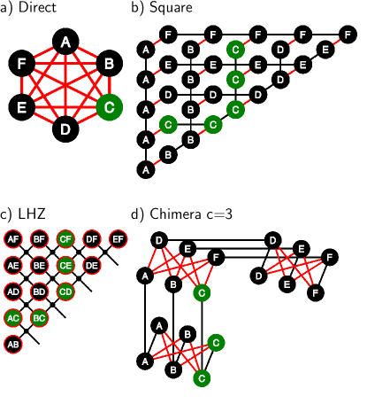
Figure 1: (a) Direct optimization. The fully connected problem with six binary variables (circles) labeled “A–F.” Couplers between the variables are represented as solid (red) lines. (b) The square lattice. The logical variable C is represented by a chain of $N-1$ logical qubits. Constraints are represented by black (dark) lines. These chains are laid out such that every variable chain can connect to every other variable chain, shown by the red (light) lines. (c) The LHZ scheme. In the PAQO embedding, a physical variable $\alpha_{i,j}$ is the product of two logical binary variables $\sigma_{i}\sigma_{j}$. The logical couplers correspond to physical local biases (red). Constraints are enforced with $4$-local interactions (black crosses) between neighboring spins. (d) The chimera lattice, $c=3$. A $K_{3,3}$ Chimera lattice consisting of a square-embedding-like chain structure (black or dark lines) combined with bipartite graph cells. These cells contain the logical couplers (red or light lines).

The paper is structured as follows. In Sec. II, we discuss the different embedding strategies analyzed in this work, and then, in Sec. III, we outline the technical details of the benchmarking. Section IV shows our main results, followed by Sec. V on embedding penalties. We summarize our findings in Sec. VI. Appendices A and B contain two technical notes about PAQO constraints and avoided level crossings.

II DETAILS ON EMBEDDING SCHEMES

In this section we describe in detail the different embedding schemes, as well as the corresponding decoding strategies. In general, we aim to optimize a binary quadratic optimization problem on a complete graph, i.e.,

$${\mathcal{H}}=\sum_{i<j}J_{ij}\sigma_{i}\sigma_{j},$$ (1)

where the variables $\sigma_{i}\in\{\pm 1\}$ and the problem is specified by the values of the couplers $J_{ij}$. Note that in this work we do not study linear terms in Eq. (1) without loss of generality.

II.1 Embedding on a square lattice

Square-lattice embedding reduces an all-to-all logical system to a physical system connected only locally. This is achieved by representing each logical variable as a chain of strongly coupled physical qubits. Figure 1(b) shows the square embedding for the example presented in Fig. 1(a). Each logical variable is represented by a chain of qubits of length $N-1$. With a careful chain layout, each chain of physical qubits has a coupler to every other chain, where the logical couplings (red, light color) are located. The black (dark) couplers along the chains are the constraints that ensure that all variables on the chain have the same value, i.e., either all up or all down. If the logical problem has a special structure or limited connectivity, the embedding of the logical problem can be optimized to use as few physical qubits as possible with the minor embedding Choi (2008). An optimal optimization, however, poses the risk of being computationally more expensive to solve than the actual optimization problem itself. Since we use heavily connected as well as all-to-all-connected problems, use of the minor embedding yields no benefits. We choose the constraints for each logical variable as

$$C_{i}(\omega,\gamma)=\omega+\gamma\sum_{j\neq i}|J_{ij}|,$$ (2)

where $\omega$ is a constant determining a fixed base constraint, while $\gamma$ is the so-called “sum constraint” that is multiplied by the sum of the absolute value of the couplers $J_{ij}$ involving variable $i$. This allows us to constrain variables with more or larger couplings more strongly than variables with fewer or smaller couplings, therefore ensuring that the system is not overconstrained. In general, one wants to use constraints that are as small as possible because large penalty terms tend to affect the performance of quantum annealing hardware com (a). However, if the constraints (penalties) are not strong enough, the chains that link physical variables to create logical counterparts have the potential to “break”, thus losing the logical information about the problem. If the decoding strategy can decode errors (broken chains), we might even deliberately choose weak constraints and fix the errors later, as this is beneficial for solving the problems faster. The chain length scales linearly with the number of variables. Similarly, if $\gamma\neq 0$, the constraints also scale linearly with the number of variables, as an increased number of variables typically increases the value of the sum in Eq. (2).

Once the logical problem is embedded in the physical system, the optimization procedure is executed. The physical solution then needs to be decoded to obtain the solution for the underlying logical system. If no constraints are broken, there is a trivial mapping from the chains to the logical variables. If constraints are broken, there are many decoding strategies for square-lattice embedding. We choose a straightforward and computationally inexpensive strategy here. For every chain, majority voting determines the value of the logical variable, depending on the value of the majority of physical variables in a chain.

II.2 Embedding on a chimera lattice

Chimera-lattice embedding Bunyk et al. (2014), which is used in the D-Wave 2000Q device, uses a variant of the aforementioned square-lattice embedding. The chimera lattice consists of bipartite unit cells of size $2c$ for some fixed integer $c$. For the D-Wave 2000Q, $c=4$. A logical variable is represented by a chain of physical qubits but it takes fewer qubits to represent the variable due to the higher connectivity in a single $K_{4,4}$ cell. Figure 1(d) shows the embedding on a $c=3$ chimera lattice for the example shown in Fig. 1(a). The cells at the bottom and on the right contain the same $c$ qubits, while all the other cells (in this example, only one) contain $2c$ unique qubits. As for embedding on the square lattice, we use majority voting for decoding. Note that the embedding strategy outlined here can also be used for the new generation of D-Wave devices, i.e., the D-Wave Advantage with the new Pegasus topology. Because the connectivity is higher, shorter chain lengths are needed. However, the lattice remains quasiplanar.

II.3 Parity adiabatic quantum optimization

An alternative way to map the logical problem has recently been proposed in Ref. Lechner et al. (2015). The PAQO or LHZ scheme encodes the logical problem differently to square- and chimera-lattice embedding. Instead of having the notion of logical variables in the physical system, each physical variable encodes the product between two logical variables $\alpha_{i,j}=\sigma_{i}\sigma_{j}$, i.e., stores if they are equal or opposite. The main advantage of this approach is the mapping from logical couplings to physical local biases, which can be controlled better than two-qubit physical couplers. Figure 1(c) shows the PAQO embedding for the example in Fig. 1(a). While the locality of the Hamiltonian goes from quadratic to quartic, a fully connected nonplanar graph turns into a square lattice. This embedding will be of considerable relevance once four-way couplers become available on quantum annealers.

The constraints are modeled as $4$-local terms com (b) between four variables that form a tile. Fixed variables that are positive can be introduced at the lower-right edge to complete tiles [not shown in Fig. 1(c)]. Because every logical variable appears twice in a constraint term, it must be $1$, i.e., for the example in Fig. 1(a),

$$\alpha_{\rm AH}\alpha_{\rm AG}\alpha_{\rm BH}\alpha_{\rm BG}=\sigma_{\rm A}\sigma_{\rm H}\sigma_{\rm A}\sigma_{\rm G}\sigma_{\rm B}\sigma_{\rm H}\sigma_{\rm B}\sigma_{\rm G}=1,$$ (3)

where $\alpha$ denotes physical variables (qubits) and $\sigma$ denotes logical variables. This that means every tile needs an even number of negative physical variables. The Hamiltonian is therefore defined as

$${\mathcal{H}_{\text{PAQO}}}=\sum_{i<j}J_{ij}\alpha_{i,j}+\sum_{l}C_{l}\leavevmode\nobreak\ \alpha_{\nwarrow}\alpha_{\swarrow}\alpha_{\searrow}\alpha_{\nearrow}$$ (4)

where $l$ iterates over all $4$-local constraints that have one physical spin in each corner and $C_{l}(\omega,\gamma)=\omega+\gamma\leavevmode\nobreak\ (J_{\nwarrow}+J_{\swarrow}+J_{\searrow}+J_{\nearrow})$, analogous to Eq. 2.

In general, the scaling of the constraints depends on the problem class and can be analytically understood for the ferromagnetic, antiferromagnetic and spin-glass cases with exponents between $0.5$-$2$ Lanthaler and Lechner (2020). Here, we choose to scale the constraints according to the worst-case scenario, i.e., $\propto N^{2}$, which is motivated in Appendix A. An alternative is to set the constraints, perform the optimization, and then verify if any of the constraints are broken. If so, increase the value and iterate. This, however, can be computationally costly.

The PAQO embedding shares similarities with a low-density parity code, which can be decoded using belief propagation, as also proposed in Ref. Pastawski and Preskill (2016). The original choice of constraints is not unique in any way; there are many combinations of physical variables that form loops, meaning that each logical variable occurs an even number of times leading the expression to be $1$. Belief propagation uses this fact and creates, for example, all possible three-variable loops, e.g., $\alpha_{AB}\alpha_{AC}\alpha_{BC}=1$ and determines which of the physical variables are most likely to be wrong in a broken constraint. While the random bit-flip error resilience of the PAQO scheme might be very useful in an implementation, it cannot correct for single broken constraints as shown in Fig. 8. Belief propagation then decodes the wrong logical state if started from Fig. 8(e) compared to Fig. 8(b). Hence, reducing the constraints is undesirable.

III METHODS

We compare the different embedding schemes using the time to solution (TTS) Rønnow et al. (2014) for quantum annealing with the goal of determining the cost overhead compared to a direct optimization of the logical problem. The TTS $s$ is defined via

$$s_{p_{\text{tar}}}(T)=Tr_{p_{\text{tar}}}(T),$$ (5)

where

$$r_{p_{\text{tar}}}(T)=\frac{\log[1-p_{\text{tar}}]}{\log[1-p_{\text{g.s.}}(T)]}$$ (6)

is the number of repetitions needed to obtain a given target success probability $p_{\text{tar}}$, $T$ is the anneal time, and $p_{\text{g.s.}}(T)$ is the probability that the ground state is found. There are two possible types of ground states that interest us, the physical one and, more importantly, the logical one. It is valuable to investigate the physical ground state, because it can be decoded trivially. The result can then be compared to that obtained by the decoder to check its performance. We use a simple grid search to determine the optimal parameters and thus extract the true scaling. This works well because $s_{p_{\text{tar}}}(T)$ is typically a convex function, as shown in Fig. 2(b). To obtain the optimal $s^{\rm opt}$ that describes the actual scaling, the TTS is minimized with respect to the anneal time $T$, i.e.,

$$s_{p_{\text{tar}}}^{\rm opt}=\min_{T}[s_{p_{\text{tar}}}(T)].$$ (7)

To keep the notation concise, we use $s_{P}=s_{90\%}^{\rm opt,physical}$ for the optimal time to solution of the physical ground state and $s_{L}=s_{90\%}^{\rm opt,logical}$ for the logical ground state after the decoder is run.

As a benchmark problem and a proxy for real-world applications, we use two instance types. First, we use unweighted MaxCut instances characterized by their connectivity density $p$, where $p=1$ ($100\%$) corresponds to an all-to-all-connected graph. Given a graph of size $N$ and density $p$, we generate instances with $N$ vertices and $N_{e}=p[N(N-1)]/2$ edges. This number is then rounded to the nearest integer. The seed $s$ initializes the random number generator that draws $N_{e}$ random edges from the set of all possible edges. All edges have an antiferromagnetic weight, i.e., $J=-1$. The second problem family class consists of all to all connected ($p=1$) instances with weights drawn from a Gaussian distribution, such that there are ferromagnetic and antiferromagnetic weights, i.e., a Gaussian Sherrington-Kirkpatrick Sherrington and Kirkpatrick (1975) spin glass.

We simulate $31$ different logical problems with size $N=5$ – $35$ variables. For each system size $N$, we generate $30$ random instances of three types: $p=0.3$ MaxCut, $p=0.5$ MaxCut, and fully connected Gaussian spin glasses with mean $\mu=0$ and variance $\sigma=1$. Using simulated quantum annealing, we study the logical problem directly, the problem embedded in a square lattice, the problem embedded on a chimera lattice and the problem encoded in the PAQO scheme. For each instance, we use $30$ repetitions of the transverse-field-simulated quantum annealing Santoro et al. (2002); Heim et al. (2015); Isakov et al. (2016); Mazzola et al. (2017) algorithm with $29$ different annealing times between $5$ and $28000$ Monte Carlo sweeps. Furthermore, we use $1024$ Trotter slices and an inverse temperature of $\beta=1024$. The transverse field (annealing schedule) is varied from $0.5$ to $0.001$ in a square manner, with the steep edge at the beginning. Multiplying all dimensions yields approximately $1.1\times 10^{7}$ simulations to be performed. To reduce the search space, we drop selected parameter combinations, e.g., a small logical problem size with a long annealing time and vice versa. This, in turn, reduces the search space to approximately $9$ million simulations. Finally, for square- and cimera-lattice embedding we use $\omega=0$ and $\gamma=1.1$ in Eq. (2), while for the PAQO scheme we use $\omega=N^{2}/50$ and $\gamma=1.1$ for the constraints.

As an example, Fig. 2(a) shows the ground-state (g.s.) hit probability for a single specific instance and different annealing times. By counting the Trotter slices that have the ground-state energy, we can compute the ground-state hit probability, because a measurement corresponds to choosing one random Trotter slice. We then convert this quantity to $s_{0.9}$ and display the result in Fig. 2(b) where $s_{0.9}^{opt}$ is marked by an arrow.

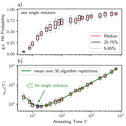
Figure 2: (a) The ground-state hit probability (g.s.-Hit) for various annealing times $T$ using simulated quantum annealing. The slower we anneal, the more likely we are to find the ground state. The specific instance used in this example is a MaxCut instance of size $N=25$ and density $p=0.3$. For each annealing time, we repeat the algorithm $30$ times. The box plot shows the first to third quartile, while the whiskers represent 5% and 95% of the measured data. (b) The time to solution (with a probability of 90%) versus the annealing time $T$. Because the ground-state hit probability is not a linear function, it is faster to repeat short-annealing-time runs than to invest in one long run. Therefore, we measure the mean and not the median. Both panels have the same horizontal axis.

Following the same procedure, we calculate $s_{0.9}^{opt}$ for every individual instance. It is quite possible that different MaxCut instances of the same size and density display their $s_{0.9}^{opt}$ at different $T$. Figure 3(a) shows these $s_{0.9}^{opt}$ versus different instance sizes. As an example, we show data for the logical problems embedded onto the chimera lattice.

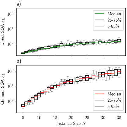
Figure 3: (a) All $s_{0.9}^{opt}$ for a physical problem using simulated quantum annealing (SQA) [one highlighted in Fig. 2(b) with a green arrow] of all instances, with density $p=0.5$ sorted by size in a linear-log box plot. (b) The same as (a), but for the problems embedded in the chimera lattice. Both panels have the same horizontal axis.

To estimate the embedding overhead, we compare the data in Fig. 3(b) (post chimera embedding) with Fig. 3(a) (direct optimization of the logical problem) by plotting $s_{0.9}^{opt}$ in a scatter plot for the different embedding schemes in Sec. IV.

IV QUANTUM MONTE CARLO RESULTS

Figure 4 shows the $s_{L}$ of the direct simulation and the three embedding schemes versus the logical system size $N$. The data clearly show a time-based penalty due to the different embedding schemes over the direct simulation of the logical problem. To better quantify the embedding overhead, we study the ratio between the TTS of the logical and physical problems. The data are shown in Fig. 5 as an instance-by-instance scatter plot. The data have an approximately linear trend (log-log plot), indicating a polynomial overhead in the time to solution.

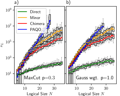
Figure 4: $s_{L}$ vs the logical system size $N$ for (a) MaxCut instances with $p=0.3$ and (b) Gaussian spin glasses. The data shown are for the three embedding schemes, as well as a direct simulation of the logical problem (bottom data set). The $s_{L}$ for each instance is determined by averaging over $30$ random starts of the algorithm. The reason for the absence of the largest system size for the PAQO scheme is the inability to find the ground state, likely due to insufficient constraint scaling. Both panels have the same vertical axis.

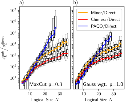
Figure 5: The same data as in Fig. 4 but divided by $s_{L}^{\rm direct}$. Both panels have the same vertical axis.

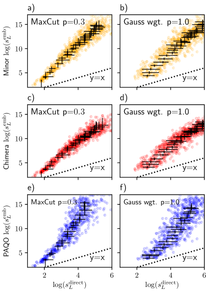
Figure 6: The same data as in Fig. 4 but displayed with $\log(s_{L})$ embedded versus direct optimization of every independent instance as a scatter plot. The black crosses show the first to third quartiles for each logical size. The linear scaling in a log-log plot indicates a polynomial scaling. All panels share the same vertical and horizontal axes.

Fitting the data in Fig. 6 to a linear function of the form $y=mx+c$ yields the parameters shown in Tab. 1. We show the fit for both $s_{L}$ and $s_{P}$. While it seems nonintuitive that $s_{L}$ scales worse than $s_{P}$, Fig. 7 shows that the decoding yields more benefits for small sizes and hence distorts the scaling. However, the actual graph of $s_{L}$ is bounded by $s_{P}$, because $s_{P}$ is trivially decodable. Therefore, the scaling of $s_{L}$ is also bounded eventually by $s_{P}$. Thus we assume the smaller scaling of the two. A stronger decoder might lead to a better scaling but most likely at a corresponding level of complexity regarding its run time.

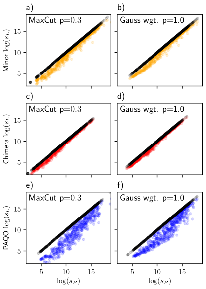
Figure 7: $s_{L}$ plotted versus $s_{P}$ for the three embedding schemes and MaxCut ($p=0.3$, left column) and Gaussian spin glasses (right column). A decoder can only make $s_{L}$ faster. If we run a trivial decoder that accepts no errors, then $s_{L}$ is equal to $s_{P}$ — shown as the black circles. A trend to smaller benefits toward larger sizes (i.e., larger $s_{P}$) is visible, which leads to slightly worse scaling when fitting the data. Furthermore, it is visible that the decoder for the PAQO scheme is more efficient than majority voting for embedding on both the square and chimera lattices. While it reduces $s_{L}$ by orders of magnitude compared to $s_{P}$—which could be invaluable for any real-world applications—it does not improve the scaling.

Table 1: The fitting parameters for a linear fitting function of the form $y=mx+c$ over the medians shown in Fig. 6. Easier instances might scale better, while harder instance families might scale considerably worse. We include the fit parameters for $s_{L}$ and $s_{P}$, together with the correlation coefficient $r$ of the linear regression.

Algorithm	Problem type	$m_{L}$	$c_{L}$	$r_{L}$	$m_{P}$	$c_{P}$	$r_{P}$
Square	MaxCut p=0.3	3.27	-2.28	1.00	2.98	-0.52	0.99
Square	MaxCut p=0.5	3.45	-2.95	0.99	3.06	-0.66	0.99
Square	Gaussian weights p=1.0	3.00	-2.92	0.99	2.70	-0.97	0.99
Chimera	MaxCut p=0.3	2.73	-1.59	1.00	2.55	-0.57	0.99
Chimera	MaxCut p=0.5	2.81	-1.72	0.99	2.57	-0.39	0.99
Chimera	Gaussian weights p=1.0	2.54	-1.95	0.99	2.35	-0.84	0.99
PAQO	MaxCut p=0.3	5.03	-7.61	0.99	3.89	-1.66	0.99
PAQO	MaxCut p=0.5	4.31	-6.05	0.99	3.80	-1.23	0.99
PAQO	Gaussian weights p=1.0	4.09	-7.62	0.98	3.35	-2.71	0.99

V A note on Embedding penalties

Both an all-to-all spin glass and the encoded spin glass suffer from an exponentially closing gap Knysh (2015). Due to the chainlike nature of the physical spins representing a logical spin, all three embeddings are subject to the fact that the gap of a ferromagnetic chain in a weak field is exponentially suppressed Isakov et al. (2016) with system size $N$. More precisely, Ref. Isakov et al. (2016) has shown the gap to be $\Delta\approx\Gamma^{N}/J^{N-1}$, where $\Gamma$ is the field strength and $J$ the ferromagnetic coupling of the chain. The gap is related to the tunneling rate to flip the chain, which determines the dynamics and hence the required annealing time $T$. The reason why the physical spin chain must be able to flip is motivated in Appendix B with a three-spin example. Furthermore, the constraint-to-logical coupling ratio worsens with growing chains, because longer chains require stronger constraints to prevent breaks. However, an embedded system using $\mathcal{O}({N^{2}})$ spins is not as slow as a native $\mathcal{O}({N^{2}})$ problem, because the constraint structure is ferromagnetic, which is easier to solve.

VI CONCLUSIONS

We study the time overhead when solving quadratic binary optimization problems using quantum annealing after embedding the problems with three different embedding schemes. In all cases, there is a sizable time overhead in the time to solution with exponents between $m=2.35$ and $m=5.03$, and an exponential slowdown with respect to the system size $N$. A constant-speed advantage of analog quantum annealers is quickly decreased and turned into a slowdown by this run-time penalty for embedding. Therefore, in the absence of long-range physical couplers that would allow for the study of problems without the need of embedding schemes in superconducting quantum annealing machines, simulated quantum annealing scales better in time to solution than analog quantum annealers with quasiplanar graph topologies. Similarly, programmable gate-model quantum computers could also implement arbitrary problems with arbitrary connectivity with only a polynomial and not an exponential overhead in the problem size $N$.

In light of these results, as far as analog quantum annealers are concerned, it is also of great interest to develop novel approaches to potentially overcome these limitations. These could include variable connectivity Hauke et al. (2015), nonlinear driving Susa and Nishimori (2020), variational quantum annealing Susa and Nishimori (2021), as well as counterdiabatic driving Hartmann and Lechner (2019). The present results could serve as a benchmark for future developments of hardware quantum annealers.

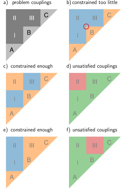
Figure 8: A constraint-scaling example in the PAQO scheme. The logical system is not shown. (a) The logical couplers are set up in three equal groups for a logical system of large size N; hence we do not display the individual physical spins as in Figure 1(c). All spins in A want to be parallel (light gray, $J=1$) to each other, as do the ones in B and C. Region I wants all A spins to be antiparallel (dark gray, $J=-1$) to all B spins. Region II is the same for all A and C spins and region III is the same for all B and C spins. (b) The physical ground state (blue down spin, orange up spin) if the $4$-local term constraint marked with the (red) circle is too weak. This broken ground state satisfies all problem couplings but does not correspond to a logical state. (c) If the constraints are strong enough, at least one of the regions is not satisfied [here, region II of area $(1/9)N^{2}$]. (d) Unsatisfied couplings from the solution in (c), where the red color marks physical spins that add energy. (e) Another possible physical ground state if constrained enough, with (f) showing the unsatisfied couplings thereof in region III, again of area $(1/9)N^{2}$.

Appendix A PAQO CONSTRAINTS

The constraints for the PAQO embedding need to be selected more carefully because a safe lower bound for the constraint strength is not immediately evident. Consider the following logical problem, which consists of $N$ all-to-all-connected spins divided into three groups, A, B, and C. Within each group, they are coupled with $J=1$ and want to be parallel. Each group is connected with $J=-1$ to any spin of the other groups, i.e. groups A, B, and C all want to be antiparallel to each other, making them frustrated amongst each other. Because it is not possible for A, B, and C to be all antiparallel, at least one pairing needs to be parallel. Figure 8 shows the corresponding PAQO embedding where allowing one broken constraint lowers the energy by $E=(1/9)N^{2}$. Note that this argument can be repeated in a recursive way in the regions A, B, and C to reach a bound of $E=(1/6)N^{2}$. This lower bound dictates the constraint to grow at least as fast to prevent being broken in the physical ground state. Because this is just one example, it is not a safe theoretical lower bound for any arbitrary problem. As such, calculating the necessary minimal constraints is more difficult than for square- and chimera-lattice embedding. We expand the analysis of Fig. 8 in Fig. 9, where we change the problem in Fig. 8(a) such that we can observe the break at every point and plot the strength required to prevent it. Again, this is one problem family with one antiferromagnetic and one ferromagnetic coupling and not a guaranteed lower bound. But if any one constraint is below this bound, we can construct an instance for which the constraints are too weak to find the proper physical ground state. The decoder might still recover from this error, but it is straightforward to construct problems where this is not the case.

Figure 9: The minimal $4$-local-term constraint strength required. Using the example from Fig. 8 and changing the number of spins in Groups A, B, and C (and therefore the size of the blocks I, II, and III) allows one to move the constraint position that breaks to any point and observe at which strength it breaks. This is mapped out in this contour plot in terms of $N^{2}$. It shows that the $4$-local-term constraint must be stronger in the middle of the PAQO embedding and can be weaker at toward the borders. This is, however, just one type of problem family and not a rigorous lower bound.

Appendix B A Note on Avoided Level Crossings

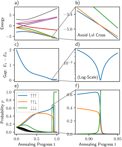
Figure 10: Spectrum, energy gap, and instantaneous ground state for a 3-spin ferromagnetic chain with individual local fields com (c). Panel (a) shows the spectrum of transverse field annealing, starting with the pure transverse field at $t=0$ and transforming to the pure problem Hamiltonian at $t=1$ in a linear manner. (b) Avoided level crossing between the two lowest states. Panel (c) show the first energy gap with a zoom in log scale shown in panel (d). The gap reaches $\Delta\approx 10^{-3}$ at its smallest position. (e) The instantaneous ground state is shown by the probabilities in the computational basis, of which we only label the three dominant parts and display the remaining five as black lines. Panel (f) shows the sudden rise and fall of the ground-state components representing a flip in the first two spins, and changing the third spin from a superposition to up.

In hard-optimization problems, avoided level crossings Knysh (2015) arise in the annealing spectrum because the driver Hamiltonian might initially favor certain configurations that become unfavorable once the driver is weak enough. To remain in the instantaneous ground state and follow the adiabatic anneal path, the spins have to flip. In contrast problems where the initial horizontal spins (due to the transverse field driver) only move toward up or down and do not need to flip during the anneal are much easier to solve . We include a three-spin example com (c) with the spectrum shown in Figs. 10(a) and 10(b) that displays such an avoided crossing at $t\approx 0.92$, where $T$ is the annealing time and $t$ is the progress in the annealing schedule. The gap in Figs. 10(c) and 10(d) shrinks linearly to near zero and then grows again. The instantaneous ground state displayed in computational-basis probabilities in Figs. 10(e) and 10(f) clearly shows that the first two spins flip from up ($p_{\text{up}}\approx 1$) to down ($p_{\text{down}}\approx 1$), while the third spin changes from a superposition to down. Figures 1(a) – 1(d) show the spins that need to be flipped if one flips the logical spin marked C. For square- and chimera-lattice embedding, it corresponds to a ferromagnetic chain that grows linearly with the system size $N$. In the PAQO scheme, we also require a number of flips that grows linearly with $N$. The physical spins are connected by $4$-local terms and hence form a chain structure as well, as can be seen in Fig. 1(c). Any embedding needs to accommodate the flips of logical spins during the anneal (ideally) in an efficient manner.

References

- Johnson et al. (2011) M. W. Johnson, M. H. S. Amin, S. Gildert, T. Lanting, F. Hamze, N. Dickson, R. Harris, A. J. Berkley, J. Johansson, P. Bunyk, et al., Quantum annealing with manufactured spins, Nature 473, 194 (2011).
- Dickson et al. (2013) N. G. Dickson, M. W. Johnson, M. H. Amin, R. Harris, F. Altomare, A. J. Berkley, P. Bunyk, J. Cai, E. M. Chapple, P. Chavez, et al., Thermally assisted quantum annealing of a 16-qubit problem, Nat. Commun. 4, 1903 (2013).
- Bunyk et al. (2014) P. Bunyk, E. Hoskinson, M. W. Johnson, E. Tolkacheva, F. Altomare, A. J. Berkley, R. Harris, J. P. Hilton, T. Lanting, and J. Whittaker, Architectural Considerations in the Design of a Superconducting Quantum Annealing Processor, IEEE Trans. Appl. Supercond. 24, 1 (2014).
- Pudenz et al. (2014) K. L. Pudenz, T. Albash, and D. A. Lidar, Error-corrected quantum annealing with hundreds of qubits, Nat. Commun. 5, 3243 (2014).
- Smith and Smolin (2013) G. Smith and J. A. Smolin, Putting “Quantumness” to the Test, Physics 6, 105 (2013).
- Boixo et al. (2013) S. Boixo, T. Albash, F. M. Spedalieri, N. Chancellor, and D. A. Lidar, Experimental signature of programmable quantum annealing, Nat. Commun. 4, 2067 (2013).
- Albash et al. (2015a) T. Albash, T. F. Rønnow, M. Troyer, and D. A. Lidar, Reexamining classical and quantum models for the D-Wave One processor, Eur. Phys. J. Spec. Top. 224, 111 (2015a).
- Rønnow et al. (2014) T. F. Rønnow, Z. Wang, J. Job, S. Boixo, S. V. Isakov, D. Wecker, J. M. Martinis, D. A. Lidar, and M. Troyer, Defining and detecting quantum speedup, Science 345, 420 (2014).
- Katzgraber et al. (2014) H. G. Katzgraber, F. Hamze, and R. S. Andrist, Glassy Chimeras Could Be Blind to Quantum Speedup: Designing Better Benchmarks for Quantum Annealing Machines, Phys. Rev. X 4, 021008 (2014).
- Lanting et al. (2014) T. Lanting, A. J. Przybysz, A. Y. Smirnov, F. M. Spedalieri, M. H. Amin, A. J. Berkley, R. Harris, F. Altomare, S. Boixo, P. Bunyk, et al., Entanglement in a quantum annealing processor, Phys. Rev. X 4, 021041 (2014).
- Santra et al. (2014) S. Santra, G. Quiroz, G. Ver Steeg, and D. A. Lidar, Max 2-SAT with up to 108 qubits, New J. Phys. 16, 045006 (2014).
- Shin et al. (2014) S. W. Shin, G. Smith, J. A. Smolin, and U. Vazirani, How “Quantum” is the D-Wave Machine? (2014), (arXiv:1401.7087).
- Vinci et al. (2014) W. Vinci, T. Albash, A. Mishra, P. A. Warburton, and D. A. Lidar, Distinguishing classical and quantum models for the D-Wave device (2014), (arXiv:1403.4228).
- Boixo et al. (2014) S. Boixo, T. F. Rønnow, S. V. Isakov, Z. Wang, D. Wecker, D. A. Lidar, J. M. Martinis, and M. Troyer, Evidence for quantum annealing with more than one hundred qubits, Nat. Phys. 10, 218 (2014).
- Albash et al. (2015b) T. Albash, W. Vinci, A. Mishra, P. A. Warburton, and D. A. Lidar, Consistency Tests of Classical and Quantum Models for a Quantum Device, Phys. Rev. A 91, 042314 (2015b).
- Albash and Lidar (2018) T. Albash and D. A. Lidar, Demonstration of a scaling advantage for a Quantum Annealer over Simulated Annealing, Phys. Rev. X 8, 031016 (2018).
- Katzgraber et al. (2015) H. G. Katzgraber, F. Hamze, Z. Zhu, A. J. Ochoa, and H. Munoz-Bauza, Seeking Quantum Speedup Through Spin Glasses: The Good, the Bad, and the Ugly, Phys. Rev. X 5, 031026 (2015).
- Martin-Mayor and Hen (2015) V. Martin-Mayor and I. Hen, Unraveling Quantum Annealers using Classical Hardness, Nature Scientific Reports 5, 15324 (2015).
- Pudenz et al. (2015) K. L. Pudenz, T. Albash, and D. A. Lidar, Quantum Annealing Correction for Random Ising Problems, Phys. Rev. A 91, 042302 (2015).
- Hen et al. (2015) I. Hen, J. Job, T. Albash, T. F. Rønnow, M. Troyer, and D. A. Lidar, Probing for quantum speedup in spin-glass problems with planted solutions, Phys. Rev. A 92, 042325 (2015).
- Venturelli et al. (2015) D. Venturelli, S. Mandrà, S. Knysh, B. O’Gorman, R. Biswas, and V. Smelyanskiy, Quantum Optimization of Fully Connected Spin Glasses, Phys. Rev. X 5, 031040 (2015).
- Vinci et al. (2015) W. Vinci, T. Albash, G. Paz-Silva, I. Hen, and D. A. Lidar, Quantum annealing correction with minor embedding, Phys. Rev. A 92, 042310 (2015).
- Zhu et al. (2016) Z. Zhu, A. J. Ochoa, F. Hamze, S. Schnabel, and H. G. Katzgraber, Best-case performance of quantum annealers on native spin-glass benchmarks: How chaos can affect success probabilities, Phys. Rev. A 93, 012317 (2016).
- Mandrà et al. (2016) S. Mandrà, Z. Zhu, W. Wang, A. Perdomo-Ortiz, and H. G. Katzgraber, Strengths and weaknesses of weak-strong cluster problems: A detailed overview of state-of-the-art classical heuristics versus quantum approaches, Phys. Rev. A 94, 022337 (2016).
- Mandrà and Katzgraber (2017) S. Mandrà and H. G. Katzgraber, The pitfalls of planar spin-glass benchmarks: Raising the bar for quantum annealers (again), Quant. Sci. Technol. 2, 038501 (2017).
- Mandrà and Katzgraber (2018) S. Mandrà and H. G. Katzgraber, A deceptive step towards quantum speedup detection, Quantum Sci. Technol. 3, 04LT01 (2018).
- Finnila et al. (1994) A. B. Finnila, M. A. Gomez, C. Sebenik, C. Stenson, and J. D. Doll, Quantum annealing: A new method for minimizing multidimensional functions, Chem. Phys. Lett. 219, 343 (1994).
- Kadowaki and Nishimori (1998) T. Kadowaki and H. Nishimori, Quantum annealing in the transverse Ising model, Phys. Rev. E 58, 5355 (1998).
- Brooke et al. (1999) J. Brooke, D. Bitko, T. F. Rosenbaum, and G. Aepli, Quantum annealing of a disordered magnet, Science 284, 779 (1999).
- Farhi et al. (2001) E. Farhi, J. Goldstone, S. Gutmann, J. Lapan, A. Lundgren, and D. Preda, A quantum adiabatic evolution algorithm applied to random instances of an NP-complete problem, Science 292, 472 (2001).
- Santoro et al. (2002) G. Santoro, E. Martoňák, R. Tosatti, and R. Car, Theory of quantum annealing of an Ising spin glass, Science 295, 2427 (2002).
- Das and Chakrabarti (2005) A. Das and B. K. Chakrabarti, Quantum Annealing and Related Optimization Methods (Edited by A. Das and B.K. Chakrabarti, Lecture Notes in Physics 679, Berlin: Springer, 2005).
- Santoro and Tosatti (2006) G. E. Santoro and E. Tosatti, TOPICAL REVIEW: Optimization using quantum mechanics: quantum annealing through adiabatic evolution, J. Phys. A 39, R393 (2006).
- Das and Chakrabarti (2008) A. Das and B. K. Chakrabarti, Quantum Annealing and Analog Quantum Computation, Rev. Mod. Phys. 80, 1061 (2008).
- Morita and Nishimori (2008) S. Morita and H. Nishimori, Mathematical Foundation of Quantum Annealing, J. Math. Phys. 49, 125210 (2008).
- Hauke et al. (2020) P. Hauke, H. G. Katzgraber, W. Lechner, H. Nishimori, and W. Oliver, Perspectives of quantum annealing: methods and implementations, Rep. Prog. Phys. 83, 054401 (2020).
- Katzgraber (2018) H. G. Katzgraber, Viewing vanilla quantum annealing through spin glasses, Quantum Science and Technology 3, 030505 (2018).
- Perdomo-Ortiz et al. (2017) A. Perdomo-Ortiz, A. Feldman, A. Ozaeta, S. V. Isakov, Z. Zhu, B. O’Gorman, H. G. Katzgraber, A. Diedrich, H. Neven, J. de Kleer, et al., On the readiness of quantum optimization machines for industrial applications (2017), arXiv:1708.09780.
- Tsukamoto et al. (2017) S. Tsukamoto, M. Takatsu, S. Matsubara, and H. Tamura, An Accelerator Architecture for Combinatorial Optimization Problems, FUJITSU Sci. Tech. J. 53, 8 (2017).
- Matsubara et al. (2017) S. Matsubara, H. Tamura, M. Takatsu, D. Yoo, B. Vatankhahghadim, H. Yamasaki, T. Miyazawa, S. Tsukamoto, Y. Watanabe, K. Takemoto, et al., in Complex, Intelligent, and Software Intensive Systems – Proceedings of the 11th International Conference on Complex, Intelligent, and Software Intensive Systems (CISIS-2017), Torino, Italy, July 10–12, 2017 (2017), p. 432.
- Aramon et al. (2018) M. Aramon, G. Rosenberg, T. Miyazawa, H. Tamura, and H. G. Katzgraber, Physics-inspired optimization for constraint-satisfaction problems using a digital annealer (2018), (arXiv:1806.08815).
- Hamerly et al. (2018) R. Hamerly, T. Inagaki, P. L. McMahon, D. Venturelli, A. Marandi, T. Onodera, E. Ng, C. Langrock, K. Inaba, T. Honjo, et al., Scaling advantages of all-to-all connectivity in physical annealers: The Coherent Ising Machine vs. D-Wave 2000Q (2018), (arXiv:quant-phys/1805.05217).
- Pastawski and Preskill (2016) F. Pastawski and J. Preskill, Error correction for encoded quantum annealing, Phys. Rev. A 93, 052325 (2016).
- Choi (2008) V. Choi, Minor-embedding in adiabatic quantum computation. I: The parameter setting problem., Quantum Inf. Process. 7, 193 (2008).
- com (a) This constraint modeling can be improved. Constraints closer to the chain end can be smaller, since they need only be stronger than the weaker part of the chain.
- Lechner et al. (2015) W. Lechner, P. Hauke, and P. Zoller, A quantum annealing architecture with all-to-all connectivity from local interactions, Science Advances 1, e1500838 (2015).
- com (b) In absence of a -local coupling therm, these constraints can be broken down into -local coupling terms by introducing further auxiliary spins.
- Lanthaler and Lechner (2020) M. Lanthaler and W. Lechner, Minimal constraints in the parity formulation of optimization problems, arXiv preprint arXiv:2008.10458 (2020).
- Sherrington and Kirkpatrick (1975) D. Sherrington and S. Kirkpatrick, Solvable model of a spin glass, Phys. Rev. Lett. 35, 1792 (1975).
- Heim et al. (2015) B. Heim, T. F. Rønnow, S. V. Isakov, and M. Troyer, Quantum versus classical annealing of Ising spin glasses, Science 348, 215 (2015).
- Isakov et al. (2016) S. V. Isakov, G. Mazzola, V. N. Smelyanskiy, Z. Jiang, S. Boixo, H. Neven, and M. Troyer, Understanding Quantum Tunneling through Quantum Monte Carlo Simulations, Phys. Rev. Lett. 117, 180402 (2016).
- Mazzola et al. (2017) G. Mazzola, V. N. Smelyanskiy, and M. Troyer, Quantum Monte Carlo tunneling from quantum chemistry to quantum annealing, Phys. Rev. B 96, 134305 (2017).
- Knysh (2015) S. Knysh, Computational Bottlenecks of Quantum Annealing (2015), (arXiv:quant-phys/1506.08608).
- Hauke et al. (2015) P. Hauke, L. Bonnes, M. Heyl, and W. Lechner, Probing entanglement in adiabatic quantum optimization with trapped ions, Frontiers in Physics 3, 21 (2015).
- Susa and Nishimori (2020) Y. Susa and H. Nishimori, Performance enhancement of quantum annealing under the lechner–hauke–zoller scheme by non-linear driving of the constraint term, Journal of the Physical Society of Japan 89, 044006 (2020).
- Susa and Nishimori (2021) Y. Susa and H. Nishimori, Variational optimization of the quantum annealing schedule for the lechner-hauke-zoller scheme, Physical Review A 103, 022619 (2021).
- Hartmann and Lechner (2019) A. Hartmann and W. Lechner, Rapid counter-diabatic sweeps in lattice gauge adiabatic quantum computing, New Journal of Physics 21, 043025 (2019).
- com (c) The coupling for the 3-spin systems are (unspecified energy unit): and the local fields are: .