Complexity of a Projected Newton-CG Method for Optimization with Bounds

Abstract

This paper describes a method for solving smooth nonconvex minimization problems subject to bound constraints with good worst-case complexity guarantees and practical performance. The method contains elements of two existing methods: the classical gradient projection approach for bound-constrained optimization and a recently proposed Newton-conjugate gradient algorithm for unconstrained nonconvex optimization. Using a new definition of approximate second-order optimality parametrized by some tolerance $\epsilon$ (which is compared with related definitions from previous works), we derive complexity bounds in terms of $\epsilon$ for both the number of iterations required and the total amount of computation. The latter is measured by the number of gradient evaluations or Hessian-vector products. We also describe illustrative computational results on several test problems from low-rank matrix optimization.

1 Introduction

We consider the problem

$$\min\,f(x)\quad\mbox{subject to}\;\;x\in\Omega,$$ (1)

where $f:\mathbb{R}^{n}\rightarrow\mathbb{R}$ is twice continuously differentiable and is bounded below by $f_{\rm low}>-\infty$ on the closed feasible set $\Omega$. We focus on $\Omega$ defined by nonnegativity constraints on a subset $\mathcal{I}$ of the variables, that is,

$$\Omega\triangleq\{x\in\mathbb{R}^{n}\mid x^{i}\geq 0,\;i\in\mathcal{I}\},\;\;\mbox{where $\mathcal{I}\subseteq\{1,2,\dotsc,n\}$.}$$ (2)

Bounds are the simplest type of inequality constraint. Euclidean projection onto the feasible set $\Omega$, a trivial operation when $\Omega$ is defined by bounds, is a fundamental component of several successful algorithms. Bound-constrained subproblems often arise in algorithms for more complicated constrained optimization problems, such as augmented Lagrangian methods. Bound constraints also appear in popular problems such as nonnegative least-squares and nonnegative matrix factorization gillis2014and . Approaches of several types have been proposed for solving this problem, including gradient projection, active set methods, and interior-point methods. See nocedal2006numerical for details.

In this paper, we describe a line-search method for solving (1), (2) that exploits the simplicity of Euclidean projection onto $\Omega$. It combines gradient projection with a Newton-conjugate gradient (Newton-CG) method for smooth nonconvex unconstrained optimization proposed recently in Royer2019 . The elements of our method are well known for their good practical performance in various optimization contexts. By combining these elements in the right way, and introducing judicious strategies for diagonal scaling, step length acceptance, and detection of negative curvature, we equip the method with a worst-case complexity theory that matches best-known theoretical bounds for bound-constrained optimization and even for unconstrained optimization. Preliminary numerical results confirm that the method has appealing practical performance. In contrast to most previous works on complexity, we prove results for both iteration and computational complexity. The latter is measured in terms of two key operations: evaluation of a gradient at a given point, and computation of a Hessian-vector product involving an arbitrary vector. (The latter is known to cost a modest multiple of a gradient evaluation when computational differentiation techniques are used griewank2008evaluating .) Our method does not require explicit calculation or storage of the Hessian; it accesses the Hessian only via products with given vectors.

Background and Prior Work.

There has been renewed interest in devising optimization algorithms with worst-case complexity guarantees for constrained nonconvex optimization. Interior-point type methods were developed to solve nonconvex problems with bound constraints Bian2015 , or with bounds and linear equality constraints Haeser2018 . A log-barrier method for bound-constrained problems was proposed in 10.1093/imanum/drz074 . Like the present paper, this method made use of the Newton-CG method of Royer2019 , but in a quite different way. An adaptive cubic regularization algorithm was proposed in cartis2012adaptive to solve nonconvex optimization with general convex constraints. Later, in cartis2015evaluation , the authors of cartis2012adaptive designed a novel two-phase target-following algorithm to address a more general problem class: nonconvex optimization with nonlinear equality constraints and a general convex feasible region. They also generalize the concept of approximate first-order optimal point to arbitrary high-order and apply a conceptual high-order algorithm for obtaining such a point cartis2018second . Authors of birgin2018regularization outline a high-order algorithm that obtains approximate first-order optimal point of a nonconvex optimization problem with general constraints. The paper cartis2019universal considered a high-order universal adaptive regularization algorithm to find approximate first-order optimal points for nonconvex problems with convex constraints, but they have even less stringent assumptions on the smoothness of the objective. Specifically, they required $q$th-order derivatives to be Hölder continuous, and they obtained complexity results that depend on the degree of smoothness and / or the regularization power (see details below). For high-order adaptive regularization methods, chen2017partially showed that the complexity may not be affected when a non-Lipschitz singular function ($l_{p}$-norm, $p\in(0,1)$) is introduced into the objective. Other works include nouiehed2020trust , which uses a trust region method to locate second-order optimal point of nonconvex problems with linear constraints. A Hessian barrier algorithm was recently proposed dvurechensky2021hessian , based on self-concordant barrier functions, which solves nonconvex problems with general conic constraints and linear equality constraints.

In these articles, good complexity results follow from the use of the Hessian and sometimes higher-order derivatives: $\mathcal{O}(\epsilon^{-3/2})$ iteration/evaluation complexity to locate an $\epsilon$-approximate first-order optimal point cartis2012adaptive ; cartis2015evaluation ; birgin2018regularization or a $(\epsilon,\sqrt{\epsilon})$ second-order optimal point Bian2015 ; Haeser2018 ; 10.1093/imanum/drz074 ; dvurechensky2021hessian ; nouiehed2020trust . (Here $\epsilon$ and $\sqrt{\epsilon}$ represent the precision of first- and second-order optimality conditions, respectively.) The $q$th-order algorithm in cartis2018second locates an $\epsilon$-approximate $q$th-order solution in $\mathcal{O}(\epsilon^{-(q+1)})$ iterations; while the $q$th-order algorithms in birgin2018regularization finds an $\epsilon$-approximate first-order solution in $\mathcal{O}(\epsilon^{-(q+1)/q})$ iterations. The algorithm that exploits the $q$th-order Taylor model in cartis2019universal locates the $\epsilon$-approximate first-order solution in $\mathcal{O}(\epsilon^{-(q+\alpha)/(q+\alpha-1)})$ iterations under the assumption that the objective’s $q$th-order derivative (with $q\geq 1$) is Hölder continuous with exponent $\alpha$ (with $0<\alpha\leq 1$) and the regularization power is high enough.

Complexity results in the works discussed above focus on iteration/evaluation complexity; less attention is paid to the bounds on the total amount of computation required. In fact, these methods can require solution of nonconvex subproblems that may themselves require a significant and undetermined amount of computation. For example, in cartis2012adaptive ; cartis2015evaluation , a potentially expensive cubic regularized subproblem (itself a constrained nonconvex problem) needs to be solved to approximate first-order optimality at each iteration, while the higher-order methods of cartis2018second , birgin2018regularization , cartis2019universal and chen2017partially require solution of subproblems involving higher-order derivatives. In nouiehed2020trust , checking the second-order stationary condition can be NP-hard, and the constrained nonconvex subproblem needs to be solved to at least first-order stationary per iteration. Moreover, implementations of these methods may require explicit evaluation of the Hessian or higher-order derivatives. The method of this paper, by contrast, requires explicit evaluation only of gradients; the Hessians are accessed only via Hessian-vector products. This fact allows us to define meaningful bounds on computational complexity.

The pursuit of optimal iteration/evaluation complexity results may compromise the practicality of algorithms. For example, subproblems in the second-order algorithms from Bian2015 and Haeser2018 have a small trust-region radius that depends on $\epsilon$. The log-barrier approach of 10.1093/imanum/drz074 has unimpressive practical performance, as we see in Section 5.

Other works that address complexity of constrained nonconvex optimization, include curtis2018complexity , which discusses the trust funnel algorithm to solve optimization with equality constraints; xie2021complexity ; grapiglia2021complexity ; birgin2020complexity ; sahin2019inexact , which discuss augmented Lagrangian methods (ALM); and lin2022complexity , concerning penalty methods. In grapiglia2021complexity , ALM and appropriate first-order algorithms to solve subproblems are utilized to locate $\epsilon$ approximate first-order point, with evaluation complexity arbitrarily close to $\mathcal{O}(\epsilon^{-4})$. Complexity of a safeguarded ALM is derived in birgin2020complexity to find first-order stationary points, but the cost of solving the subproblems is not well defined. In lin2022complexity , complexity results are established in terms of the number of proximal gradient steps needed to find an $\epsilon$ first-order stationary points. The complexity can be improved to $\mathcal{O}(\epsilon^{-5/2})$ (omitting logarithm terms) when the constraint functions are convex and Slater’s condition holds. curtis2018complexity ; xie2021complexity ; sahin2019inexact consider optimization with equality constraints that do not accommodate the bound-constrained problem class (1), (2).

A complicating factor in comparing complexity of methods for finding approximate optimal points is that the definitions of such points vary between papers. This is not unexpected since different papers consider a variety of constraint types, and the approximate optimality conditions are adapted to the particular formulations. The relation between different definitions has not been discussed in any detail, even for the case of optimization with bounds. We believe that a proper discussion facilitates a better understanding of the goals and characteristics of different algorithms.

Approach and Contributions.

We describe an algorithm for locating an approximate second-order point of the problem (1),(2) that has good worst-case complexity bounds — similar to the unconstrained case ($\Omega=\mathbb{R}^{n}$ in (1)) — and is also practical.

As a preliminary to our description of the algorithm, we state our definition of approximate second-order optimality, alongside four other definitions that have appeared in the literature. These definitions are typically parametrized by a tolerance $\epsilon$. We introduce a second parameter $p$ that represents the power of $\epsilon$ that determines the approximate condition involving the Hessian, and refer to the resulting conditions as “$(\epsilon,p)$-second-order optimality” or “$(\epsilon,p)$-2o” for short. The alternative definitions that we discuss in this article are based on those from cartis2018second ; Haeser2018 ; 10.1093/imanum/drz074 ; Bian2015 , specialized to the bound-constrained problem (1),(2), with $\mathcal{I}=\{1,\ldots,n\}$. We make comparisons among all these definitions, using a new notion of “essentially stronger”.

Practical methods that make use of gradient projection and Newton scaling have yet to be considered seriously as methods with good complexity guarantees for bound-constrained problems. Such methods exploit the simplicity of the projection operation for $\Omega$ in (2), as well as the benefits of second-order information that have been shown in the unconstrained context. The two-metric projection framework proposed by Bertsekas bertsekas1982projected ; bertsekas2014constrained provides a potential framework, for appropriate choice of scaling matrix. This method takes steps of the form

$$x_{k+1}\triangleq P(x_{k}-\alpha_{k}D_{k}\nabla f(x_{k})),$$ (3)

where $D_{k}$ is a symmetric positive definite matrix (with a certain structure defined below) and $P(z)$ is the projection onto the feasible set $\Omega$ in (2), defined by

$$[P(z)]^{i}=\begin{cases}\max\{z^{i},0\}&\;\;i\in\mathcal{I},\\ z^{i}&\;\;\mbox{\rm otherwise.}\end{cases}$$ (4)

The matrix $D_{k}$ scales the free and active parts of the gradient differently, in a way that guarantees decrease in the objective function for sufficiently small positive steplengths $\alpha_{k}$. Denoting a set of “apparently-active” components of $x_{k}$ by

$$I_{k}^{+}(\epsilon_{k})\triangleq\{i\in\mathcal{I}\mid 0\leq x_{k}^{i}\leq\epsilon_{k},\;\nabla_{i}f(x_{k})>0\},$$ (5)

for small positive $\epsilon_{k}$, $D_{k}$ is assumed to be positive diagonal in the $I_{k}^{+}(\epsilon_{k})$ components, that is, $D_{k}[i,j]=0$ if either $i$ or $j$ is in $I_{k}^{+}(\epsilon_{k})$ with $j\neq i$, and $D_{k}[i,i]>0$ for all $i\in I_{k}^{+}(\epsilon_{k})$. The two-metric projection method can have rapid convergence when $f(x)$ is convex and the square submatrix of $D_{k}$ for the “apparently-free” indices $i\notin I_{k}^{+}(\epsilon_{k})$ is derived from the corresponding submatrix of the Hessian $\nabla^{2}f(x_{k})$. The complexity properties of this method in the setting of nonconvex $f$ are the subject of ongoing work.

Inspired by both two-metric gradient projection approach and the Newton-CG algorithm for unconstrained optimization described in Royer2019 , we propose a projected Newton-CG algorithm. We show that the algorithm terminates within $\mathcal{O}(\epsilon^{-3/2})$ iterations and outputs an $(\epsilon,\tfrac{1}{2})$-2o point with high probability. In each iteration of the projected Newton-CG, we either (1) take a gradient projection step; (2) take a projected Newton-CG step, obtained via a capped CG procedure applied to the apparently-free components, or (3) take a projected step along a negative curvature direction of a diagonally scaled Hessian. The operations required to calculate each type of step are well defined, and are similar to those used in Royer2019 ; doi:10.1137/17M1134329 . These “fundamental operations” are of two types: (1) a gradient calculation, and (2) computation of the product of the Hessian with an arbitrary vector — an operation that does not require explicit computation or knowledge of the Hessian and that can be performed at roughly equivalent cost to a gradient evaluation; see griewank2008evaluating . The other potentially significant computations are (1) function evaluations performed during the backtracking line searches, the number of which is bounded by an $O(\log\epsilon)$ multiple of the number of gradient evaluations, and which are usually significantly cheaper than gradient evaluations; and (2) vector operations involving vectors of length $n$ (inner products and saxpys), whose $\mathcal{O}(n)$ cost is dominated by the cost of the fundamental operations for all functions of interest. By contrast, other methods require solution of potentially expensive constrained nonconvex subproblems in each iteration birgin2018regularization ; cartis2012adaptive ; cartis2015evaluation ; cartis2018second and possibly explicit evaluation of Hessians and higher derivatives. These requirements have the potential to make the computational complexity less competitive.

Table 1 shows iteration/evaluation complexity and operation complexity results for our algorithm (last row) and existing algorithms, based on their respective definitions of $(\epsilon,p)$-2o. The “operation complexity” results are upper bounds on the number of fundamental operations required to find an approximate solution.

Table 1: Complexity estimates for nonconvex optimization procedures involving bounds.

Definition of $(\epsilon,p)$-2o∗	$\begin{array}[]{l}\mbox{Iteration/evaluation}\\ \mbox{Complexity }\end{array}$	$\begin{array}[]{l}\mbox{Operation}\\ \mbox{Complexity }(p=\tfrac{1}{2})\end{array}$	Ref.
(12)	$\mathcal{O}(\epsilon^{-3})^{\star\star}$ $(p=1)$	$-$	cartis2018second
(13)	$\mathcal{O}(\epsilon^{-3/2})$ $(p=1/2)$	$-$	Haeser2018
(14)	$\begin{array}[]{l}\tilde{\mathcal{O}}(n\epsilon^{-1/2}+\epsilon^{-3/2})^{\dagger}\\ (p=1/2)\end{array}$	$\begin{array}[]{l}\tilde{\mathcal{O}}(n\epsilon^{-3/4}+\epsilon^{-7/4}),\mbox{$n$ large}\\ \tilde{\mathcal{O}}(n\epsilon^{-3/2}),\mbox{$n$ small}\end{array}$	10.1093/imanum/drz074
(15)	$\mathcal{O}(\epsilon^{-3/2})$ $(p=1/2)$	$-$	Bian2015
(9) w. $\mathcal{I}=\{1,\ldots,n\}$	$\mathcal{O}(\epsilon^{-3/2})$ $(p=1/2)$	$\mathcal{O}(\epsilon^{-3/2}\min\{n,\epsilon^{-1/4}\log(\frac{n}{\epsilon\delta})\})$	(here)

$*$: Definition of $(\epsilon,p)$-2o is based on the paper in “Ref.” but tailored to problem (1),(2) with $\mathcal{I}=\{1,\ldots,n\}$.
$\star\star$: When $p=1$, accuracy on the optimality condition involving Hessian is higher, leading to a higher complexity bound.
$\dagger$: $\tilde{\mathcal{O}}$ represents $\mathcal{O}$ with logarithmic factors omitted.

Illustrative numerical experiments on nonnegative matrix factorization problems show that the projected Newton-CG algorithm has good practical performance: It contends well with gradient projection method and the log-barrier Newton-CG algorithm proposed in 10.1093/imanum/drz074 , and is comparable to approaches that are specialized to this problem in relatively low dimensions.

With minor modifications (c.f. Appendix D), the projected Newton-CG can be applied to problems with two-sided bounds, where $\Omega$ is redefined as $\{x\in\mathbb{R}^{n}\mid 0\leq x^{i}\leq u^{i},i\in\mathcal{I}\}$, $\mathcal{I}\subseteq\{1,2,\ldots,n\}$, with the same complexity guarantees.

Organization.

In Section 2, we introduce some basic assumptions and definitions to be used throughout the article. Definitions of the approximate second-order optimal point in our work and others are discussed in Section 3. The projected Newton-CG is presented and analyzed in Section 4. Section 5 describes numerical experiments. Section 6 contains some concluding remarks.

We include in the Appendix details of the relationship between different definitions of approximate second-order optimality, the oracles utilized in the projected Newton-CG algorithm, and extension to two-sided bounds.

2 Preliminaries

We summarize here some notations, two assumptions used throughout the paper, and (exact) optimality conditions for (1), (2).

Notation.

We use subscripts for iteration numbers (usually $k$) throughout, and denote components of vectors by superscripts and components of matrices using square-bracket notation, with $[i,j]$ denotes the $i,j$ element. We use the following notation for gradient and Hessian of $f$ at $x_{k}$:

$$g_{k}\triangleq\nabla f(x_{k}),\quad H_{k}\triangleq\nabla^{2}f(x_{k}).$$

We use $\nabla_{i}f(x)$ to denote the $i$th component of $\nabla f(x)$. $\mathop{\hbox{\rm diag}}(v)$ is a diagonal matrix with $v^{i}$ being its $[i,i]$ element. $\mathop{\hbox{\rm sgn}}(z)=1$ if $z\geq 0$ and $\mathop{\hbox{\rm sgn}}(z)=-1$ otherwise. $\|\cdot\|$ denotes the 2-norm of a vector or a matrix. $c_{+}\triangleq\max\{c,0\}$ for a scalar $c\in\mathbb{R}$. $\mathcal{I}^{c}\triangleq\{1,\ldots,n\}\setminus\mathcal{I}$. $P(\cdot)$ denotes the projection onto the feasible region $\Omega$.

Assumptions.

The following assumptions are used throughout the paper, though they are not mentioned explicitly in the statements of some lemmas.

Assumption 1

The level set $\mathcal{L}_{f}(x_{0})\triangleq\{x\in\mathbb{R}^{n}\mid x\in\Omega,\;f(x)\leq f(x_{0})\}$ is compact.

Assumption 2

$f$ is twice Lipschitz continuously differentiable on an open convex set containing $\mathcal{L}_{f}(x_{0})$ and all the trial points generated by Algorithm 1.

Lipschitz constants for $f$, $\nabla f(x)$ and $\nabla^{2}f(x)$ on the set described in Assumption 2 are denoted by $L_{f}$, $L_{g}$ and $L_{H}$, respectively. Thus, for any $x,v\in\mathbb{R}^{n}$ such that $x$ and $x+v$ are in this set, we have

$$f(x+v)\leq f(x)+L_{f}\|v\|,$$ (6a)

$$f(x+v)\leq f(x)+\nabla f(x)^{T}v+\frac{L_{g}}{2}\|v\|^{2},$$ (6b)

$$f(x+v)\leq f(x)+\nabla f(x)^{T}v+\frac{1}{2}v^{T}\nabla^{2}f(x)v+\frac{L_{H}}{6}\|v\|^{3}.$$ (6c)

Therefore, $\|\nabla f(x)\|\leq L_{f}$ and $\|\nabla^{2}f(x)\|\leq L_{g}$ over $\mathcal{L}_{f}(x_{0})$.

Optimality Conditions.

We can write first-order optimality conditions for (1), (2) (also known as stationarity conditions) at a point $\bar{x}$ as follows:

$$\begin{aligned} &\bar{x}^{i}\geq 0,\quad\nabla_{i}f(\bar{x})\geq 0,\;\quad\forall i\in\mathcal{I};\\ &\nabla_{i}f(\bar{x})=0,\quad\forall i\in\mathcal{I}^{c}\cup\{i\in\mathcal{I}\mid\bar{x}^{i}>0\}.\end{aligned}$$ (7)

A weak second-order condition for (1), (2) is that the two-sided projection of $\nabla^{2}f(\bar{x})$ onto the variables $i$ such that $\bar{x}^{i}>0$ or $i\in\mathcal{I}^{c}$ is positive semidefinite, which is equivalent to

$$z^{T}\nabla^{2}f(\bar{x})z\geq 0,\quad\forall z\in\{z\in\mathbb{R}^{n}\mid z^{i}=0,i\in\{i\in\mathcal{I}\mid\bar{x}^{i}=0\}\}.$$ (8)

This condition coincides with the usual second-order necessary condition where there are no “degenerate” indices, that is, indices $i\in\mathcal{I}$ for which both $\bar{x}^{i}=0$ and $\nabla_{i}f(\bar{x})=0$. When such indices exist, a standard second-order necessary condition is:

$$z^{T}\nabla^{2}f(\bar{x})z\geq 0,\quad\forall z\in\left\{z\in\mathbb{R}^{n}\Big{|}\begin{array}[]{cc}z^{i}=0,&\mbox{if}\;i\in\mathcal{I},\bar{x}^{i}=0,\nabla_{i}f(\bar{x})>0,\\ z^{i}\geq 0&\mbox{if}\;i\in\mathcal{I},\bar{x}^{i}=0,\nabla_{i}f(\bar{x})=0.\end{array}\right\}.$$

However, checking this condition can be as hard as checking copositivity of a matrix, which is NP-hard. Thus, as in previous works (such as 10.1093/imanum/drz074 ), we base our analysis on the less stringent condition (8).

3 Approximate second-order optimal points

In this section we give our definition of $(\epsilon,p)$-approximate second-order optimal points and compare it with similar definitions in the literature. For simplicity of notation, we use $(\epsilon,p)$-2o points to denote $(\epsilon,p)$-approximate second-order optimal points. We assume $\epsilon,p>0$ throughout.

Our definition of an $(\epsilon,p)$-2o point is as follows.

Definition 1 (($\epsilon,p$)-2o, Def1)

$x$ is an ($\epsilon,p$)-2o point of (1),(2) according to Def1 if $x\in\Omega$ and for sets $J^{+}$ and $J^{-}$ defined by

$$J^{+} \triangleq\{i\in\mathcal{I}\mid 0\leq x^{i}\leq\sqrt{\epsilon}\},$$

$$J^{-} \triangleq\{1,\ldots,n\}\setminus J^{+}=\mathcal{I}^{c}\cup\{i\in\mathcal{I}\mid x^{i}>\sqrt{\epsilon}\},$$

and for diagonal matrix $S=\mathop{\hbox{\rm diag}}(s)$ with $s^{i}=1$ when $i\in J^{-}$ and $s^{i}=x^{i}$ when $i\in J^{+}$, we have

$$\|S\nabla f(x)\|\leq 2\epsilon,\quad\nabla_{i}f(x)\geq-\epsilon^{3/4},\,\mbox{\rm for all $i\in J^{+}$,}$$ (9a)

$$S\nabla^{2}f(x)S\succeq-\epsilon^{p}I.$$ (9b)

Definition 1 is motivated by the (weak) second-order optimal conditions (7) and (8). In fact, if we let $\epsilon=0$, then the $(0,p)$-2o point satisfies (7) and (8) exactly. The following lemma further justifies Definition 1 and our purpose to find an $(\epsilon,p)$-2o point given small $\epsilon$.

Lemma 1

Consider problem (1),(2). Suppose we have a positive scalar sequence $\{\epsilon_{k}\}$ with $\epsilon_{k}\downarrow 0$ and vector sequence $\{x_{k}\}\subseteq\Omega$ with $x_{k}\rightarrow x^{*}$ such that $x_{k}$ is an $(\epsilon_{k},p)$-2o point according to Definition 1. Then $x^{*}$ satisfies second-order optimal conditions (7), (8). That is, for sets $\mathcal{J}_{*}^{-}$ and $\mathcal{J}_{*}^{-}$ defined by

$$\mathcal{J}_{*}^{-}\triangleq\mathcal{I}_{c}\cup\{i\in\mathcal{I}\mid(x^{*})^{i}>0\},\quad\mathcal{J}_{*}^{+}\triangleq\{1,2,\ldots,n\}\setminus\mathcal{J}_{*}^{-},$$

we have

$$(x^{*})^{i}\geq 0,\quad\nabla_{i}f(x^{*})\geq 0,\quad \forall i\in\mathcal{I};$$ (10a)

$$\nabla_{i}f(x^{*})=0,\quad \forall i\in\mathcal{J}_{*}^{-};$$ (10b)

$$z^{T}\nabla^{2}f(x^{*})z\geq 0,\quad \forall z\in\{z\in\mathbb{R}^{n}\mid z^{i}=0,\,i\in\mathcal{J}_{*}^{+}\}.$$ (10c)

Proof

Denote sets $\mathcal{J}_{k}^{+}$, $\mathcal{J}_{k}^{-}$ and diagonal matrix $\mathcal{S}_{k}=\mathop{\hbox{\rm diag}}(s_{k})$ which correspond to $J^{+}$, $J^{-}$, and $S$ in Definition 1 with $x=x_{k}$, $\epsilon=\epsilon_{k}$ and $s=s_{k}$. Note that since $x_{k}\to x^{*}$ and $\epsilon_{k}\downarrow 0$, there exists $\bar{k}$ such that for any $k>\bar{k}$, we have $\mathcal{J}_{k}^{+}\subseteq\mathcal{J}_{*}^{+}$, $\mathcal{J}_{*}^{-}\subseteq\mathcal{J}_{k}^{-}$. Our claim that $x^{*}$ satisfies (10) is a consequence of the following four observations.

• Feasibility of $x^{*}$ follows from closedness of $\Omega$.

• For any $i\in\mathcal{I}$ and any $k$, either $i\in\mathcal{J}_{k}^{+}$ so $\nabla_{i}f(x_{k})\geq-\epsilon_{k}^{3/4}$, or $i\in\mathcal{J}_{k}^{-}$ so $|\nabla_{i}f(x_{k})|\leq 2\epsilon_{k}\implies\nabla_{i}f(x_{k})\geq-2\epsilon_{k}$. By taking limits, we have $\nabla_{i}f(x^{*})\geq 0$.

• Fix any $i\in\mathcal{J}_{*}^{-}$. For all $k>\bar{k}$, we have $i\in\mathcal{J}_{k}^{-}$. Therefore, $s_{k}^{i}=1$ and $|\nabla_{i}f(x_{k})|\leq 2\epsilon_{k}$. By taking limits, we have $\nabla_{i}f(x^{*})=0$.

• Fix any $z\in\{z\in\mathbb{R}^{n}\mid z^{i}=0,i\in\mathcal{J}_{*}^{+}\}$. For all $k>\bar{k}$, we have $i\in\mathcal{J}_{k}^{+}\implies i\in\mathcal{J}_{*}^{+}\implies z^{i}=0$, so that $\mathcal{S}_{k}z=z$. Since $z^{T}\mathcal{S}_{k}\nabla^{2}f(x_{k})\mathcal{S}_{k}z\geq-\epsilon_{k}^{p}\|z\|^{2}$ for any $k$, we have by taking limits that $z^{T}\nabla^{2}f(x^{*})z\geq 0$.

∎

We now identify several definitions of approximate second-order optimal conditions proposed in literature and discuss their relationship. For simplicity, we assume in the rest of this section that

$$\mathcal{I}\triangleq\{1,2,\ldots,n\},$$ (11)

(so that $\Omega=\mathbb{R}^{n}_{+}$, the nonnegative orthant). When we refer to Definition 1 or Def1 in the rest of this section, we implicitly assume that (11) holds.

We start from a definition in cartis2018second , which is defined for optimization with general convex constraints and high-order optimal points. Here we tailor it to fit the scope of this paper: second-order optimal points and bound-constrained optimization: (1), (2), (11).

Definition 2 (cartis2018second , Def2)

$x$ is an $(\epsilon,p)$-2o point of (1), (2), (11) according to Def2 if $x\geq 0$ and, for some user-defined constant $\Delta_{\max}$ that is independent of $x$ and $\epsilon$, there exists $\Delta\in(0,\Delta_{\max}]$ such that

$$\begin{aligned} \left|\mbox{globalmin}_{x+d\in\Omega,\|d\|\leq\Delta}\quad\nabla f(x)^{T}d\right|&\leq\Delta\epsilon,\\ \left|\mbox{globalmin}_{x+d\in\Omega,\|d\|\leq\Delta}\quad\nabla f(x)^{T}d+\frac{1}{2}d^{T}\nabla^{2}f(x)d\right|&\leq\Delta^{2}\epsilon^{p}.\end{aligned}$$ (12)

$\Delta_{\max}$ is often chosen to reduce the effort in global minimization.

The following three definitions are from Haeser2018 ; 10.1093/imanum/drz074 ; Bian2015 tailored to our problem of interest. Here we let $X=\mathop{\hbox{\rm diag}}(x)$, $\bar{X}=\mathop{\hbox{\rm diag}}(\min\{x,{\bf 1}\})$ and ${\bf 1}$ denotes the vectors with all elements being $1$.

Definition 3 (Haeser2018 , Def3)

$x$ is an $(\epsilon,p)$-2o point of (1), (2), (11) according to Def3 if

$$\begin{aligned} x\geq 0,\;\nabla f(x)\geq-\epsilon{\bf 1},\;\|X\nabla f(x)\|_{\infty}&\leq\epsilon,\\ X\nabla^{2}f(x)X&\succeq-\epsilon^{p}I_{n}.\end{aligned}$$ (13)

Definition 4 (10.1093/imanum/drz074 , Def4)

$x$ is an $(\epsilon,p)$-2o point of (1), (2), (11) according to Def4 if

$$\begin{aligned} x\geq 0,\;\nabla f(x)\geq-\epsilon{\bf 1},\;\|\bar{X}\nabla f(x)\|_{\infty}&\leq\epsilon,\\ \bar{X}\nabla^{2}f(x)\bar{X}&\succeq-\epsilon^{p}I_{n}.\end{aligned}$$ (14)

Definition 5 (Bian2015 , Def5)

$x$ is an $(\epsilon,p)$-2o point of (1), (2), (11) according to Def5 if

$$\begin{aligned} x\geq 0,\;\|X\nabla f(x)\|_{\infty}&\leq\epsilon,\\ X\nabla^{2}f(x)X&\succeq-\epsilon^{p}I_{n}.\end{aligned}$$ (15)

The relationship between each of these definitions and second-order criticality has been discussed in the respective work. In order to discuss the relation between any two of these definitions including ours, we propose the following concept, which relates pairs of definitions of $(\epsilon,p)$-2o under the assumption that $x$ is confined to a compact set $\mathcal{X}$.

Definition 6

We say that DefA is essentially stronger than DefB on $\mathcal{X}$ if given any sufficiently small $\epsilon\in(0,1]$, any $(\epsilon,p)$-2o point $x\in\mathcal{X}$ by DefA is also a $(c\epsilon,p)$-2o point by DefB, where $c>0$ is a constant independent of $\epsilon$ or $x$. We denote this relation as $\text{\bf DefA}\gtrsim_{f,\mathcal{X},p}\text{\bf DefB}$, simplified as $\text{\bf DefA}\gtrsim\text{\bf DefB}$. We say that DefA and DefB are essentially equivalent (denoted $\text{\bf DefA}\thickapprox\text{\bf DefB}$) if $\text{\bf DefA}\gtrsim\text{\bf DefB}$ and $\text{\bf DefB}\gtrsim\text{\bf DefA}$.

Transitivity of the relation $\gtrsim$ is shown in Lemma 6.

Comparison and evaluation of complexity of different algorithms makes more sense if we are able to relate the guarantees on the points they produce according to the relations in Definition 6. In fact, if we care most about the complexity as a function of the accuracy parameter $\epsilon$, Definition 6 is natural and intuitive due to the following theorem.

Theorem 3.1

Given any $\epsilon>0$ sufficiently small, suppose that an algorithm can find an $(\epsilon,p)$-2o point $x\in\mathcal{X}$ by DefA in $\mathcal{O}(\epsilon^{-q})$ iterations ($q>0$) and $\text{\bf DefA}\gtrsim\text{\bf DefB}$. Then the algorithm can also locate an $(\epsilon,p)$-2o point by DefB in $\mathcal{O}(\epsilon^{-q})$ iterations.

Proof

Since $\text{\bf DefA}\gtrsim\text{\bf DefB}$, there is a constant $c>0$ such that for all $\epsilon>0$ sufficiently small, an $(\epsilon/c,p)$-2o point by DefA is an $(\epsilon,p)$-2o point by DefB. By assumption, the algorithm can an locate $(\epsilon/c,p)$-2o point by DefA in $\mathcal{O}((\epsilon/c)^{-q})=\mathcal{O}(\epsilon^{-q})$ number of iterations. The result follows. ∎

We can now clarify several pairwise relations between the Definitions 1-5. The proof of the following result appears in Appendix A.

Theorem 3.2

Suppose that $\mathcal{X}$ is a compact set. Then we have the following.

1. $\text{\bf Def2}\gtrsim\text{\bf Def3}$.

2. $\text{\bf Def3}\thickapprox\text{\bf Def4}$.

3. $\text{\bf Def4}\gtrsim\text{\bf Def5}$.

4. $\text{\bf Def1}\gtrsim\text{\bf Def5}$.

The assumption in Theorem 3.2 on compactness of $\mathcal{X}$ is mild. In fact, many works in literature assume that the iterates generated by their algorithms lie in a compact region, for example, the sublevel set of the objective function. By Theorem 3.2, we have the following relation chart of Definition 1-Definition 5:

$$\text{\bf Def2}\gtrsim\text{\bf Def3}\thickapprox\text{\bf Def4}\gtrsim\text{\bf Def5},\quad\text{\bf Def1}\gtrsim\text{\bf Def5}.$$

Note that each $\gtrsim$ relation above is probably strict. For example, Def2 considers the global minimum of the first-order and second-order Taylor expansions of $f$ over a small trust region, while Def3 (in fact all other definitions) is only closely related to the weak second-order necessary conditions (7),(8) for $x$ being a local minimal point. Def5 is weaker than others since it does not offer an appropriate lower bound on $\nabla_{i}f(x)$ when $x^{i}=0$. In fact, the relation between Def5 and second-order criticality is also weaker than others. Unfortunately, we cannot describe by $\gtrsim$ the relation between our definition (Def1) with definitions other than Def5. On one hand, the condition $\nabla_{i}f(x)\geq-\epsilon^{-3/4},i\in J^{+}$ in Def1 is weaker; on the other hand, the condition $\|S\nabla f(x)\|\leq 2c\epsilon$ is strong and cannot be implied by other $(\epsilon,p)$-2o definitions for any constant $c$ independent of $\epsilon$. An illustrative example is given in Appendix A, Example 1.

During the review process, we found that the definition used in nouiehed2020trust is also relevant. When tailored to the scope in this paper (see Definition 7 in Appendix A), it can be placed between Def2 and Def3 (see Theorem A.1 Appendix A).

4 Projected Newton-CG method and its complexity

We now describe a projected Newton-CG algorithm to find an $(\epsilon,\tfrac{1}{2})$-2o point according to Definition 1 for problem (1), (2), and analyze its complexity properties.

4.1 Description of the Algorithm

Given the sequence of iterates $\{x_{k}\}$ and a positive scalar sequence $\{\epsilon_{k}\}$ we define the following index sets inspired by the two-metric projection method (3), (5):

$$J_{k}^{+} \triangleq\{i\in\mathcal{I}\mid 0\leq x_{k}^{i}\leq\epsilon_{k}\},$$ (16)

$$J_{k}^{-} \triangleq\{1,\ldots,n\}\setminus J_{k}^{+}=\mathcal{I}^{c}\cup\{i\in\mathcal{I}\mid x_{k}^{i}>\epsilon_{k}\}.$$

Let $g^{-}_{k}$, $H^{-}_{k}$ be the subvector and square submatrix of $g_{k}$ and $H_{k}$, resp., corresponding to index set $J_{k}^{-}$. Similarly, we use $g^{+}_{k}$ and $H^{+}_{k}$ for the subvector and square submatrix of $g_{k}$ and $H_{k}$, resp., corresponding to index set $J_{k}^{+}$. For search direction $d_{k}$, denote $d_{k}^{-}$ and $d_{k}^{+}$ in the same fashion. Define the scaling vector $s_{k}$ and diagonal scaling matrix $S_{k}$ as follows:

$$s^{i}_{k}\triangleq\begin{cases}x_{k}^{i},\;&i\in J_{k}^{+}\\ 1,\;&i\in J_{k}^{-}\end{cases},\quad S_{k}\triangleq\mathop{\hbox{\rm diag}}(s_{k}).$$ (17)

We can then define the projected Newton-CG algorithm as Algorithm 1.

Algorithm 1 Projected Newton-CG (PNCG)

  (Initialization) Choose an initial point $x_{0}\geq 0$, tolerance $\epsilon_{g}>0$, scalar sequence $\{\epsilon_{k}\}$ with $\epsilon_{k}\in(0,1)$ for all $k$, backtracking parameters $\theta\in(0,1)$, accuracy parameter $\zeta\in(0,1)$, step acceptance parameter $\eta\in\left(0,\frac{1-\zeta}{2}\right)$.

  for $k=0,1,2,\dotsc$ do

     if $J_{k}^{+}\neq\emptyset$ and ( $g_{k}^{i}<-\epsilon_{k}^{3/2}$ for some $i\in J_{k}^{+}$ or $\|S^{+}_{k}g^{+}_{k}\|>\epsilon_{k}^{2}$ ) then

        (Gradient Projection step) Let $d_{k}:=-g_{k}$;

        Let $\tilde{m}_{k}$ be the smallest nonnegative integer $m$ such that

$$f(P(x_{k}+\theta^{m}d_{k}))<f(x_{k})-\frac{1}{2}(x_{k}-P(x_{k}+\theta^{m}d_{k}))^{T}g_{k};$$

        Let $x_{k+1}:=P(x_{k}+\theta^{\tilde{m}_{k}}d_{k})$;

     else if  $J_{k}^{-}\neq\emptyset$ and $\|g^{-}_{k}\|>\epsilon_{g}$ then

        (Newton-CG step) Call Algorithm 3 (Capped CG, Appendix B) with $H:=H^{-}_{k}$, $\epsilon:=\epsilon_{k}$, $g:=g^{-}_{k}$, accuracy parameter $\zeta$ and upper bound $M$ on Hessian norm (if provided). Obtain outputs $t\in\mathbb{R}^{|J_{k}^{-}|}$ and $d{\_\rm type}$;

        if $d\_{\rm type}={\rm NC}$ then

           Let $d^{-}_{k}:=-{\rm sgn}(t^{T}g^{-}_{k})\frac{|t^{T}H^{-}_{k}t|}{\|t\|^{2}}\frac{t}{\|t\|}$; (Negative curvature direction)

        else

           Let $d^{-}_{k}:=t$; (Approx. solution to reduced Newton equations)

        end if

        Let $d^{+}_{k}=0$ (Complete $d_{k}$ with zeros in the active components)

        Let $m_{k}$ be smallest nonnegative integer $m$ such that

$$f(P(x_{k}+\theta^{m}d_{k}))<f(x_{k})-\eta\theta^{2m}\epsilon_{k}\|d_{k}\|^{2};$$

        Let $\alpha_{k}:=\theta^{m_{k}}$, $x_{k+1}:=P(x_{k}+\theta^{m_{k}}d_{k})$;

     else

        Call Procedure 4 (Minimum Eigenvalue Oracle (MEO), Appendix C) with $H:=S_{k}H_{k}S_{k}$, $\epsilon:=\epsilon_{k}$ and the upper bound of norm of $H$ if known.

        if Procedure 4 certifies that $S_{k}H_{k}S_{k}\succeq-\epsilon_{k}I$ then

           STOP and output $x_{k}$;

        end if

        (Negative curvature step) Let $d_{k}:=-\mathop{\hbox{\rm sgn}}(g_{k}^{T}S_{k}d)\cdot|d^{T}S_{k}H_{k}S_{k}d|\cdot d$, where $d$ is the output of Procedure 4;

        Let $\bar{m}_{k}$ be the smallest nonnegative integer $m$ such that

$$f(P(x_{k}+\theta^{m}S_{k}d_{k}))<f(x_{k})-\eta\theta^{2m}\|d_{k}\|^{3}.$$

        Let $x_{k+1}:=P(x_{k}+\theta^{\bar{m}_{k}}S_{k}d_{k})$;

     end if

  end for

Elements of Algorithm 1.

As in the two-metric projection method (3), our method starts each iteration by partitioning the components of $x$ into the “apparently-free” and “apparently-active” indices based on their proximity to the boundary and a threshold parameter $\epsilon_{k}$. Then one of three types of steps is taken. For all such steps, backtracking in combination with projection onto the feasible set is used to determine an appropriate steplength.

• Gradient projection step: If examination of the gradient components corresponding to the apparently-active components indicate that a significant improvement in $f$ can be obtained by taking a standard gradient projection step, such a step is taken.

• Newton-CG step on apparently-free components: When the gradient corresponding to the apparently-free components is above the threshold $\epsilon_{g}$, the Capped CG procedure (c.f. Appendix B) is called to either find an approximate Newton step in these components, or else return a direction of negative curvature. Only the apparently-free components are modified in a step of this type.

• Scaled negative curvature step (full-dimensional): When neither of the two types of steps defined above is deemed appropriate, the current iterate $x_{k}$ satisfies the approximate optimality conditions of Definition 1, except for the condition (9b) on the scaled Hessian. We therefore check this condition and, if it is not satisfied, find a scaled negative curvature step that will lead to a significant decrease in $f$. While the other type of negative curvature step (obtained from Capped CG) changes only the apparently-free components, this scaled negative curvature step changes all components, in general. We believe that this type of step will rarely be taken; most instances of negative curvature will be detected during computation of the Newton-CG step.

Connections to known methods for bound-constrained and unconstrained optimization.

The way in which Algorithm 1 combines Newton-CG steps with gradient projection steps is inspired in part by Moré and Toraldo More91GPCG , who use CG iterations applied to the Newton system to “explore” a face of the feasible orthant and gradient projection to move to a new face. However, More91GPCG addresses only convex quadratic problems and has no complexity analysis.

There are obvious connections between Algorithm 1 and the Newton-CG methods for unconstrained nonconvex optimization described in Royer2019 and doi:10.1137/17M1134329 . The latter methods make use of Capped CG procedures (where the ”cap” refers to an implicit bound on the number of CG iterations allowed at each invocation), as well as negative curvature directions and backtracking line searches. We leverage the similarities by using the same “subroutines” for Capped CG and negative curvature detection as in Royer2019 ; these methods are stated for completeness in Appendices B and C, along with their key properties. However, the modifications required to adapt the approach of Royer2019 to handle bound constraints, in a way that allows complexity results to be proved, are significant and non-obvious. For one thing, we cannot simply project the approximate Newton step onto the feasible region, as this may not yield descent even for convex $f$; see (bertsekas2014constrained, , Section 1.5). Indeed, Bertsekas proposed the two-metric gradient projection approach precisely to deal with this issue. Essentially, the proximity of iterates $x_{k}$ to the boundary of the feasible set $\Omega$ and the use of projection inhibit steps in ways that may prevent the “significant decrease” in objective $f$ required at each iteration to prove complexity. We need to use scaling of steps and Hessians, modified steplength acceptance criteria, and novel partitions of the set of components to overcome this potential hazard. Differences with prior work, particularly the unconstrained Newton-CG approach of Royer2019 , can be summarized as follows.

1. Our partition of $\{1,2,\dotsc,n\}$ into apparently-active and apparently-free parts (16) differs from standard two-metric gradient projection in not considering the sign of the gradient.

2. We use a gradient projection step in certain conditions; devising these conditions in such a way that the step yields the significant improvement in $f$ required by our complexity analysis (see Lemma 2) is somewhat intricate.

3. We utilize a different sufficient decrease criterion for the Newton-CG step from the one in Royer2019 , and this step takes place only in the subspace of apparently-free variables. The analysis in proofs of Lemmas 3 and 4 is similar to that of corresponding results in Royer2019 , but takes the presence of bound constraints in the apparently-free variables into account.

4. We compute the full-dimensional negative curvature direction on a diagonally scaled version of the Hessian, and need a scaled direction and a different sufficient decrease condition from Royer2019 .

4.2 Complexity of Algorithm 1

The following four results — Lemmas 2 to 5 — prove a lower bound on the amount of decrease in $f$ at a single iteration in each of the following four cases. (We assume that Assumptions 1 and 2 hold with $\Omega$ in (2) for all these results, although we do not mention them in the statement of each result.)

• A gradient projection step is taken (Lemma 2);

• The Newton-CG step is triggered and the Capped CG algorithm returns $d\_{\rm type}={\rm NC}$, resulting in a negative curvature step involving the apparently-free components (Lemma 3);

• The Newton-CG step is triggered and the Capped CG algorithm returns $d\_{\rm type}={\rm SOL}$, resulting in a Newton-like step (Lemma 4);

• The MEO procedure returns a negative curvature direction instead of a certificate of optimality, and a negative curvature step is taken (Lemma 5).

We state and prove these results without further elaboration.

Lemma 2

Suppose that $J_{k}^{+}\neq\emptyset$ at iteration $k$, and that $g_{k}^{i}<-\epsilon_{k}^{3/2}$ for some $i\in J_{k}^{+}$ or $\|S^{+}_{k}g^{+}_{k}\|>\epsilon_{k}^{2}$, so that a projected gradient step is taken. Then

$$f(x_{k})-f(x_{k+1})>\frac{1}{4}\min\{\theta/L_{g},1\}\epsilon_{k}^{3}.$$

Proof

If $g_{k}^{i}<-\epsilon_{k}^{3/2}$ for some $i\in J_{k}^{+}$ or $\|S^{+}_{k}g^{+}_{k}\|>\epsilon_{k}^{2}$ at the gradient projection step, then for any steplength $\beta>0$, at least one of two cases occurs. In the first case of $g_{k}^{i}<-\epsilon_{k}^{3/2}$ for some $i\in J_{k}^{+}$, we have

$$g_{k}^{i}<-\epsilon_{k}^{3/2}\implies(g_{k}^{i})^{2}>\epsilon_{k}^{3}\implies(x_{k}^{i}-(x_{k}^{i}-\beta g_{k}^{i})_{+})g_{k}^{i}=\beta(g_{k}^{i})^{2}>\beta\epsilon_{k}^{3}.$$ (18)

In the second case, we have

$$\|S^{+}_{k}g^{+}_{k}\|^{2}>\epsilon_{k}^{4} \implies\sum_{i\in J_{k}^{+}}(x_{k}^{i})^{2}(g_{k}^{i})^{2}>\epsilon_{k}^{4}$$

$$\implies\sum_{i\in J_{k}^{+},\beta g_{k}^{i}\leq x_{k}^{i}}(x_{k}^{i})^{2}(g_{k}^{i})^{2}+\sum_{i\in J_{k}^{+},\beta g_{k}^{i}>x_{k}^{i}}(x_{k}^{i})^{2}(g_{k}^{i})^{2}>\epsilon_{k}^{4}.$$

Therefore, either

$$\sum_{i\in J_{k}^{+},\beta g_{k}^{i}\leq x_{k}^{i}}(x_{k}^{i})^{2}(g_{k}^{i})^{2}\geq\epsilon_{k}^{4}/2\overset{(x_{k}^{i}\leq\epsilon_{k},\forall i\in J_{k}^{+})}{\implies}\sum_{i\in J_{k}^{+},\beta g_{k}^{i}\leq x_{k}^{i}}(g_{k}^{i})^{2}\geq\epsilon_{k}^{2}/2,$$

or

$$\sum_{i\in J_{k}^{+},\beta g_{k}^{i}>x_{k}^{i}}(x_{k}^{i})^{2}(g_{k}^{i})^{2}\geq\epsilon_{k}^{4}/2\implies\sum_{i\in J_{k}^{+},\beta g_{k}^{i}>x_{k}^{i}}x_{k}^{i}g_{k}^{i}\geq\epsilon_{k}^{2}/\sqrt{2}.$$

Thus in this case, we have

$$\sum_{i\in J_{k}^{+}}(x_{k}^{i}-(x_{k}^{i}-\beta g_{k}^{i})_{+})g_{k}^{i} =\sum_{i\in J_{k}^{+},\beta g_{k}^{i}\leq x_{k}^{i}}\beta(g_{k}^{i})^{2}+\sum_{i\in J_{k}^{+},\beta g_{k}^{i}>x_{k}^{i}}x_{k}^{i}g_{k}^{i}$$

$$\geq\min\{\beta/2,1/\sqrt{2}\}\epsilon_{k}^{2}$$

$$\overset{(\epsilon_{k}<1)}{>}\min\{\beta/2,1/\sqrt{2}\}\epsilon_{k}^{3}.$$ (19)

By noting $g_{k}^{i}(x_{k}^{i}-(x_{k}^{i}-\beta g_{k}^{i})_{+})\geq 0$ for any $i\in\mathcal{I}$, we have for any $\beta>0$ that

$$g_{k}^{T}(x_{k}-P(x_{k}-\beta g_{k})) =\sum_{i\in\mathcal{I}}g_{k}^{i}(x_{k}^{i}-(x_{k}^{i}-\beta g_{k}^{i})_{+})+\sum_{i\in\mathcal{I}^{c}}\beta(g_{k}^{i})^{2}$$

$$\geq\sum_{i\in J_{k}^{+}}g_{k}^{i}(x_{k}^{i}-(x_{k}^{i}-\beta g_{k}^{i})_{+})$$

$$\overset{\eqref{ineq: dec.1},\eqref{ineq: dec.2}}{>}\min\{\beta/2,1/\sqrt{2}\}\epsilon_{k}^{3}.$$ (20)

Note for any $0<\beta<\frac{1}{L_{g}}$, where $L_{g}$ is the Lipschitz constant of $\nabla f$, we have

$$f(P(x_{k}-\beta g_{k})) \leq f(x_{k})-g_{k}^{T}(x_{k}-P(x_{k}-\beta g_{k}))+\frac{L_{g}}{2}\|x_{k}-P(x_{k}-\beta g_{k})\|^{2}$$

$$\leq f(x_{k})-g_{k}^{T}(x_{k}-P(x_{k}-\beta g_{k}))+\frac{L_{g}}{2}\beta g_{k}^{T}(x_{k}-P(x_{k}-\beta g_{k}))$$

$$<{\color[rgb]{0,0,0}f(x_{k})-g_{k}^{T}(x_{k}-P(x_{k}-\beta g_{k}))+\frac{1}{2}g_{k}^{T}(x_{k}-P(x_{k}-\beta g_{k}))}$$

$$=f(x_{k})-\frac{1}{2}g_{k}^{T}(x_{k}-P(x_{k}-\beta g_{k})),$$

where the second inequality holds because $(u-v)^{T}(P(u)-P(v))\geq\|P(u)-P(v)\|^{2}$ for any $u,v\in\mathbb{R}^{n}$, and the third inequality holds because $\beta<1/L_{g}$ and $g_{k}^{T}(x_{k}-P(x_{k}-\beta g_{k}))>0$ by (20). Therefore, by the line search rule, $\tilde{m}_{k}<+\infty$ and $\theta^{\tilde{m}_{k}}\geq\min\left\{\frac{\theta}{L_{g}},1\right\}$. Thus, by the lower bound for $\theta^{\tilde{m}_{k}}$, the bound (20), and the backtracking line search mechanism, we have

$$f(x_{k})-f(x_{k+1}) >\frac{1}{2}g_{k}^{T}(x_{k}-P(x_{k}-\theta^{\tilde{m}_{k}}g_{k}))>\frac{1}{4}\min\left\{\theta/L_{g},1\right\}\epsilon_{k}^{3}.$$

∎

Lemma 3

Suppose that at iteration $k$, a Newton-CG step is triggered and that Algorithm 3 returns $d\_{\rm type}={\rm NC}$. Then we have $m_{k}<+\infty$ and

$$f(x_{k})-f(P(x_{k}+\alpha_{k}d_{k}))>c_{\textnormal{nc}}\epsilon_{k}^{3},$$

where $c_{\textnormal{nc}}\triangleq\eta\min\left\{\frac{(3-6\eta)^{2}\theta^{2}}{L_{H}^{2}},\theta^{2}\right\}$.

Proof

For the Newton-CG step, if $\|\alpha d_{k}\|\leq\epsilon_{k}$ for some $\alpha>0$, then $\|\alpha d^{-}_{k}\|_{\infty}=\|\alpha d_{k}\|_{\infty}\leq\epsilon_{k}$ and $P(x_{k}+\alpha d_{k})=x_{k}+\alpha d_{k}$. From (6c), we have

$$f(P(x_{k}+\alpha d_{k})) =f(x_{k}+\alpha d_{k})$$

$$\leq f(x_{k})+\alpha g_{k}^{T}d_{k}+\frac{\alpha^{2}}{2}d_{k}^{T}H_{k}d_{k}+\frac{L_{H}}{6}\alpha^{3}\|d_{k}\|^{3}.$$ (21)

Since $d\_{\rm type}={\rm NC}$, we have that $(d^{-}_{k})^{T}g^{-}_{k}\leq 0$, and from Lemma 7(let $\bar{d}=d_{k}^{-}$,$\epsilon=\epsilon_{k}$) that $\frac{(d^{-}_{k})^{T}H^{-}_{k}d^{-}_{k}}{\|d^{-}_{k}\|^{2}}=-\|d^{-}_{k}\|\leq-\epsilon_{k}$. Then for any $0<\alpha<\frac{3-6\eta}{L_{H}}$,

$$f(x_{k})+\alpha g_{k}^{T}d_{k}+\frac{\alpha^{2}}{2}d_{k}^{T}H_{k}d_{k}+\frac{L_{H}}{6}\alpha^{3}\|d_{k}\|^{3}$$

$$=f(x_{k})+\alpha(g^{-}_{k})^{T}d^{-}_{k}+\frac{\alpha^{2}}{2}(d^{-}_{k})^{T}H^{-}_{k}d^{-}_{k}+\frac{L_{H}}{6}\alpha^{3}\|d^{-}_{k}\|^{3}$$

$$\leq f(x_{k})-\frac{\alpha^{2}}{2}\|d^{-}_{k}\|^{3}+\frac{L_{H}}{6}\alpha^{3}\|d^{-}_{k}\|^{3}$$

$$<f(x_{k})-\eta\alpha^{2}\|d^{-}_{k}\|^{3}\leq f(x_{k})-\eta\alpha^{2}\epsilon_{k}\|d_{k}\|^{2}.$$ (22)

Then, by leveraging (21) and (22), we have that if $\alpha<\min\left\{\frac{3-6\eta}{L_{H}},\frac{\epsilon_{k}}{\|d_{k}\|}\right\}$, then $f(P(x_{k}+\alpha d_{k}))<f(x_{k})-\eta\alpha^{2}\epsilon_{k}\|d_{k}\|^{2}$. Therefore, backtracking will terminate when $\alpha_{k}$ drops below $\min\left\{\frac{3-6\eta}{L_{H}},\frac{\epsilon_{k}}{\|d_{k}\|}\right\}$, if not earlier. Further, because of the backtracking mechanism, $\alpha_{k}$ cannot be less than $\theta$ times this value. As a result, we have

$$\alpha_{k}\geq \min\left\{\theta\min\left\{\frac{3-6\eta}{L_{H}},\frac{\epsilon_{k}}{\|d_{k}\|}\right\},1\right\}$$

$$\implies\alpha_{k}\|d_{k}\|\geq \min\left\{\frac{(3-6\eta)\theta\|d_{k}\|}{L_{H}},\theta\epsilon_{k},\|d_{k}\|\right\}$$

$$\overset{(\|d_{k}\|\geq\epsilon_{k})}{\geq} \min\left\{\frac{(3-6\eta)\theta}{L_{H}},\theta,1\right\}\epsilon_{k}$$

$$\implies\alpha_{k}^{2}\epsilon_{k}\|d_{k}\|^{2}\geq \min\left\{\frac{(3-6\eta)^{2}\theta^{2}}{L_{H}^{2}},\theta^{2}\right\}\epsilon_{k}^{3}.$$

Also, $\|d_{k}\|=\|d^{-}_{k}\|=\frac{|(d^{-}_{k})^{T}H^{-}_{k}d^{-}_{k}|}{\|d^{-}_{k}\|^{2}}\leq\|H^{-}_{k}\|_{2}\leq\|H_{k}\|_{2}\leq L_{g}$ and

$$\alpha_{k}\geq\min\left\{\theta\min\left\{\frac{3-6\eta}{L_{H}},\frac{\epsilon_{k}}{\|d_{k}\|}\right\},1\right\}\overset{(\|d_{k}\|\leq L_{g})}{\geq}\min\left\{\frac{(3-6\eta)\theta}{L_{H}},\frac{\theta\epsilon_{k}}{L_{g}},1\right\}$$

$$\implies m_{k}=\log_{\theta}\alpha_{k}\leq\max\left\{\log_{\theta}\left(\frac{(3-6\eta)\theta}{L_{H}}\right),\log_{\theta}\left(\frac{\theta\epsilon_{k}}{L_{g}}\right),0\right\},$$

verifying that $m_{k}$ is finite and completing the proof.∎

Lemma 4

Suppose that at iteration $k$, a Newton-CG step is triggered. Moreover, Algorithm 3 returns $d\_{\rm type}={\rm SOL}$. Then $m_{k}<+\infty$ and

$$f(x_{k})-f(P(x_{k}+\alpha_{k}d_{k}))>c_{\textnormal{sol}}\min\{\|\nabla f(P(x_{k}+\alpha_{k}d_{k}))\mid_{J_{k}^{-}}\|^{2}\epsilon_{k}^{-1},\epsilon_{k}^{3}\},$$ (23)

where

$$c_{\textnormal{sol}}\triangleq\eta\min\left\{\frac{4}{25+8L_{H}},\theta^{2},\frac{9(1-\zeta-2\eta)^{2}\theta^{2}}{L_{H}^{2}},\frac{(1-\zeta)^{2}\theta^{2}}{(L_{H}/3+2\eta)^{2}}\right\}.$$

Proof

Define

$$l_{k}\triangleq\min\left\{l\in\mathbb{N}\mid\theta^{l}\|d_{k}\|\leq\epsilon_{k}\right\}$$

$$j_{k}\triangleq$$

$$\min\left\{j\geq l_{k},j\in\mathbb{N}\mid\theta^{j}g_{k}^{T}d_{k}+\frac{\theta^{2j}}{2}d_{k}^{T}H_{k}d_{k}+\frac{L_{H}\theta^{3j}}{6}\|d_{k}\|^{3}<-\eta\theta^{2j}\epsilon_{k}\|d_{k}\|^{2}\right\}.$$

Then from (21) and the definition of $j_{k}$, we have that

$$f(P(x_{k}+\theta^{j_{k}}d_{k}))<f(x_{k})-\eta\theta^{2j_{k}}\epsilon_{k}\|d_{k}\|^{2}.$$

Therefore, by the definition of $m_{k}$ in Algorithm 1, it follows that $m_{k}\leq j_{k}$. By Lemma 7($d=d_{k}^{-}$, $g=g_{k}^{-}$, $\epsilon=\epsilon_{k}$), we have

$$\|d_{k}\|=\|d^{-}_{k}\|\leq 1.1\epsilon_{k}^{-1}\|g^{-}_{k}\|\leq 1.1\epsilon_{k}^{-1}\|g_{k}\|\leq 1.1\epsilon_{k}^{-1}L_{f},$$

so that

$$l_{k}\leq\left[\log_{\theta}\left(\frac{\epsilon_{k}}{\|d_{k}\|}\right)\right]_{+}+1\leq\left[\log_{\theta}\left(\frac{\epsilon_{k}^{2}}{1.1L_{f}}\right)\right]_{+}+1.$$ (24)

According to Lemma 7 (with $d=d_{k}^{-}$, $H=H_{k}^{-}$, $g=g_{k}^{-}$, $\epsilon=\epsilon_{k}$), we have that

$$(d_{k}^{-})^{T}(H_{k}^{-}+2\epsilon_{k}I)d_{k}^{-} \geq\epsilon_{k}\|d_{k}^{-}\|^{2},$$ (25a)

$$\|r_{k}^{-}\| \leq\frac{1}{2}\epsilon_{k}\zeta\|d_{k}^{-}\|,$$ (25b)

where $r_{k}^{-}\triangleq(H_{k}^{-}+2\epsilon_{k}I)d_{k}^{-}+g_{k}^{-}$. Then,

$$\theta^{j}(g_{k}^{-})^{T}d_{k}^{-}+\frac{\theta^{2j}}{2}(d_{k}^{-})^{T}H_{k}^{-}d_{k}^{-}+\frac{L_{H}\theta^{3j}}{6}\|d_{k}^{-}\|^{3}$$

$$=-\theta^{j}(H_{k}^{-}d_{k}^{-}+2\epsilon_{k}d_{k}^{-}-r_{k}^{-})^{T}d_{k}^{-}+\frac{\theta^{2j}}{2}(d_{k}^{-})^{T}H_{k}^{-}d_{k}^{-}+\frac{L_{H}\theta^{3j}}{6}\|d_{k}^{-}\|^{3}$$

$$=-\theta^{j}\left(1-\frac{\theta^{j}}{2}\right)(d_{k}^{-})^{T}(H_{k}^{-}+2\epsilon_{k}I)d_{k}^{-}-\epsilon_{k}\theta^{2j}\|d_{k}^{-}\|^{2}-\theta^{j}(r_{k}^{-})^{T}d_{k}^{-}$$

$$+\frac{L_{H}\theta^{3j}}{6}\|d_{k}^{-}\|^{3}$$

$$\overset{\eqref{ineq1: royer19}}{\leq}-\theta^{j}\left(1-\frac{\theta^{j}}{2}\right)\epsilon_{k}\|d_{k}^{-}\|^{2}+\theta^{j}\|r_{k}^{-}\|\|d_{k}^{-}\|+\frac{L_{H}\theta^{3j}}{6}\|d_{k}^{-}\|^{3}$$

$$\overset{\eqref{ineq2: royer19}}{\leq}-\frac{\theta^{j}}{2}\epsilon_{k}\|d_{k}^{-}\|^{2}+\frac{\theta^{j}}{2}\epsilon_{k}\zeta\|d_{k}^{-}\|^{2}+\frac{L_{H}\theta^{3j}}{6}\|d_{k}^{-}\|^{3}$$

$$=-\frac{\theta^{j}}{2}(1-\zeta)\epsilon_{k}\|d_{k}^{-}\|^{2}+\frac{L_{H}\theta^{3j}}{6}\|d_{k}^{-}\|^{3}.$$ (26)

It can be verified that for any $j\geq\left[\log_{\theta}\left(\frac{(1-\zeta)\epsilon_{k}}{\eta\epsilon_{k}+\sqrt{\eta^{2}\epsilon_{k}^{2}+1.1L_{H}(1-\zeta)L_{f}/3}}\right)\right]_{+}+1$, we have

$$\theta^{j}<\frac{(1-\zeta)\epsilon_{k}}{\eta\epsilon_{k}+\sqrt{\eta^{2}\epsilon_{k}^{2}+1.1L_{H}(1-\zeta)L_{f}/3}}$$

$$\overset{(\|d^{-}_{k}\|\leq 1.1\epsilon_{k}^{-1}L_{f})}{\implies} \theta^{j}<\frac{(1-\zeta)\epsilon_{k}}{\eta\epsilon_{k}+\sqrt{\eta^{2}\epsilon_{k}^{2}+L_{H}(1-\zeta)\epsilon_{k}\|d^{-}_{k}\|/3}}.$$

It then follows from the quadratic formula applied to the following quadratic inequality in $\theta^{j}$,

$$\frac{L_{H}\|d^{-}_{k}\|}{6}\theta^{2j}+\eta\epsilon_{k}\theta^{j}-\frac{(1-\zeta)\epsilon_{k}}{2} <0$$

$$\implies -\frac{\theta^{j}}{2}(1-\zeta)\epsilon_{k}\|d^{-}_{k}\|^{2}+\frac{L_{H}}{6}\theta^{3j}\|d^{-}_{k}\|^{3} <-\eta\theta^{2j}\epsilon_{k}\|d^{-}_{k}\|^{2}$$

$$\overset{\eqref{ineq: CR}}{\implies} \theta^{j}(g^{-}_{k})^{T}d^{-}_{k}+\frac{\theta^{2j}}{2}(d^{-}_{k})^{T}H^{-}_{k}d^{-}_{k}+\frac{L_{H}\theta^{3j}}{6}\|d^{-}_{k}\|^{3} <-\eta\theta^{2j}\epsilon_{k}\|d^{-}_{k}\|^{2}$$

$$\implies \theta^{j}g_{k}^{T}d_{k}+\frac{\theta^{2j}}{2}d_{k}^{T}H_{k}d_{k}+\frac{L_{H}\theta^{3j}}{6}\|d_{k}\|^{3} <-\eta\theta^{2j}\epsilon_{k}\|d_{k}\|^{2}.$$

Then by the definitions of $j_{k}$ and $l_{k}$ together with (24), we have

$$j_{k}\leq 1+$$

$$\max\left\{\left[\log_{\theta}\left(\frac{\epsilon_{k}^{2}}{1.1L_{f}}\right)\right]_{+},\left[\log_{\theta}\left(\frac{(1-\zeta)\epsilon_{k}}{\eta\epsilon_{k}+\sqrt{\eta^{2}\epsilon_{k}^{2}+1.1L_{H}(1-\zeta)L_{f}/3}}\right)\right]_{+}\right\},$$

which is also an upper bound for $m_{k}$.

Next, we derive the lower bound for $\alpha_{k}^{2}\epsilon_{k}\|d_{k}\|^{2}$ which, when scaled by $\eta$, is the required amount of decrease in $f$. We consider four cases.

Case 1. $j_{k}=l_{k}=0$. In this case we have $m_{k}=0$, $\alpha_{k}=1$, and $\|d^{-}_{k}\|=\|d_{k}\|\leq\epsilon_{k}$. Therefore, $x_{k}^{i}+d_{k}^{i}\geq 0,\forall i\in\mathcal{I}\cap J_{k}^{-}\implies P(x_{k}+\alpha_{k}d_{k})=x_{k}+d_{k}$. Then we have

$$\|\nabla f(P(x_{k}+\alpha_{k}d_{k}))\mid_{J_{k}^{-}}\| =\|\nabla f(x_{k}+d_{k})\mid_{J_{k}^{-}}\|$$

$$=\|\nabla f(x_{k}+d_{k})\mid_{J_{k}^{-}}-g_{k}^{-}+g_{k}^{-}\|$$

$$=\|\nabla f(x_{k}+d_{k})\mid_{J_{k}^{-}}-g_{k}^{-}-H_{k}^{-}d_{k}^{-}-2\epsilon_{k}d_{k}^{-}+r_{k}^{-}\|$$

$$\leq\frac{L_{H}}{2}\|d_{k}^{-}\|^{2}+2\epsilon_{k}\|d_{k}^{-}\|+\|r_{k}^{-}\|$$

$$\overset{\eqref{ineq2: royer19}}{\leq}\frac{L_{H}}{2}\|d_{k}^{-}\|^{2}+\frac{4+\zeta}{2}\epsilon_{k}\|d_{k}^{-}\|$$

$${\color[rgb]{0,0,0}\overset{(\zeta<1)}{\leq}\frac{L_{H}}{2}\|d_{k}^{-}\|^{2}+\frac{5}{2}\epsilon_{k}\|d_{k}^{-}\|}.$$

By applying the quadratic formula to the inequality above (which involves a quadratic in $\|d^{-}_{k}\|$), we obtain

$$\|d^{-}_{k}\| \geq\frac{-\frac{5}{2}+\sqrt{\frac{25}{4}+2L_{H}\|\nabla f(P(x_{k}+\alpha_{k}d_{k}))\mid_{J_{k}^{-}}\|/\epsilon_{k}^{2}}}{L_{H}}\cdot\epsilon_{k}$$

$$=\frac{-5+\sqrt{25+8L_{H}\min\{\|\nabla f(P(x_{k}+\alpha_{k}d_{k}))\mid_{J_{k}^{-}}\|/\epsilon_{k}^{2},1\}}}{2L_{H}}\cdot\epsilon_{k}$$

$$=\frac{4\min\{\|\nabla f(P(x_{k}+\alpha_{k}d_{k}))\mid_{J_{k}^{-}}\|/\epsilon_{k}^{2},1\}}{5+\sqrt{25+8L_{H}\min\{\|\nabla f(P(x_{k}+\alpha_{k}d_{k}))\mid_{J_{k}^{-}}\|/\epsilon_{k}^{2},1\}}}\cdot\epsilon_{k}$$

$$\geq\frac{4}{5+\sqrt{25+8L_{H}}}\min\{\|\nabla f(P(x_{k}+\alpha_{k}d_{k}))\mid_{J_{k}^{-}}\|\epsilon_{k}^{-1},\epsilon_{k}\}$$

$$\geq\frac{2}{\sqrt{25+8L_{H}}}\min\{\|\nabla f(P(x_{k}+\alpha_{k}d_{k}))\mid_{J_{k}^{-}}\|\epsilon_{k}^{-1},\epsilon_{k}\}$$

$$\Downarrow(\alpha_{k}=1,\|d_{k}\|=\|d^{-}_{k}\|)$$

$$\alpha_{k}^{2}\epsilon_{k}\|d_{k}\|^{2} \geq\frac{4}{25+8L_{H}}\min\{\|\nabla f(P(x_{k}+\alpha_{k}d_{k}))\mid_{J_{k}^{-}}\|^{2}\epsilon_{k}^{-1},\epsilon_{k}^{3}\}.$$

Case 2. $j_{k}=l_{k}\geq 1$. In this case, since $\alpha_{k}=\theta^{m_{k}}$ with $m_{k}\leq j_{k}=l_{k}$, we have

$$\theta^{l_{k}}\|d_{k}\|>\theta\epsilon_{k} \implies\alpha_{k}\|d_{k}\|=\theta^{m_{k}}\|d_{k}\|>\theta\epsilon_{k}$$

$$\implies\alpha_{k}^{2}\epsilon_{k}\|d_{k}\|^{2}=(\alpha_{k}\|d_{k}\|)^{2}\epsilon_{k}>\theta^{2}\epsilon_{k}^{3}.$$

Case 3. $j_{k}>l_{k}=0$. For $j=0$ and $j=j_{k}-1$, we must have

$$\theta^{j}g_{k}^{T}d_{k}+\frac{\theta^{2j}}{2}d_{k}^{T}H_{k}d_{k}+\frac{L_{H}\theta^{3j}}{6}\|d_{k}\|^{3}\geq-\eta\theta^{2j}\epsilon_{k}\|d_{k}\|^{2}$$

$$\implies \theta^{j}(g^{-}_{k})^{T}d^{-}_{k}+\frac{\theta^{2j}}{2}(d^{-}_{k})^{T}H^{-}_{k}d^{-}_{k}+\frac{L_{H}\theta^{3j}}{6}\|d^{-}_{k}\|^{3}\geq-\eta\theta^{2j}\epsilon_{k}\|d^{-}_{k}\|^{2}$$

$$\overset{\eqref{ineq: CR}}{\implies} -\frac{\theta^{j}}{2}(1-\zeta)\epsilon_{k}\|d^{-}_{k}\|^{2}+\frac{L_{H}}{6}\theta^{3j}\|d^{-}_{k}\|^{3}\geq-\eta\theta^{2j}\epsilon_{k}\|d^{-}_{k}\|^{2}$$

$$\implies \frac{L_{H}}{6}\theta^{2j}+\frac{\eta\epsilon_{k}}{\|d^{-}_{k}\|}\theta^{j}-\frac{(1-\zeta)\epsilon_{k}}{2\|d^{-}_{k}\|}\geq 0.$$ (27)

By setting $j=0$ in this inequality, we have $\|d^{-}_{k}\|\geq(3(1-\zeta)-6\eta)\epsilon_{k}/L_{H}$. By setting $j=j_{k}-1$ in this same inequality, and using $\theta^{j_{k}}>\theta^{2j_{k}}$, we have

$$\left(\frac{L_{H}}{6}+\frac{\eta\epsilon_{k}}{\|d^{-}_{k}\|}\right)\theta^{j_{k}-1} \geq\frac{(1-\zeta)\epsilon_{k}}{2\|d^{-}_{k}\|}$$

$$\implies\theta^{j_{k}}\|d^{-}_{k}\| \geq\frac{(1-\zeta)\theta\epsilon_{k}}{(L_{H}/3)+2\eta\epsilon_{k}/\|d^{-}_{k}\|}$$ (28)

$$\geq\frac{(1-\zeta)\theta\epsilon_{k}}{(L_{H}/3)+2\eta L_{H}/(3(1-\zeta)-6\eta)}$$

$$=\frac{3(1-\zeta-2\eta)\theta\epsilon_{k}}{L_{H}},$$

where the final equality follows by elementary manipulation. Using again $\alpha_{k}=\theta^{m_{k}}\geq\theta^{j_{k}}$, we have

$$\alpha_{k}^{2}\epsilon_{k}\|d_{k}\|^{2}=\alpha_{k}^{2}\epsilon_{k}\|d^{-}_{k}\|^{2}\geq(\theta^{j_{k}}\|d^{-}_{k}\|)^{2}\epsilon_{k}\geq\frac{9(1-\zeta-2\eta)^{2}\theta^{2}\epsilon_{k}^{3}}{L_{H}^{2}}.$$

Case 4. $j_{k}>l_{k}\geq 1$. By the same argument as in Case 3, (28) holds. Moreover, $\|d^{-}_{k}\|=\|d_{k}\|>\epsilon_{k}$ since $l_{k}\geq 1$. Therefore, we have

$$\eqref{ineq: pp8} \implies\theta^{j_{k}}\|d^{-}_{k}\|\geq\frac{(1-\zeta)\theta\epsilon_{k}}{L_{H}/3+2\eta\epsilon_{k}/\|d^{-}_{k}\|}>\frac{(1-\zeta)\theta\epsilon_{k}}{L_{H}/3+2\eta}$$

$$\implies\alpha_{k}^{2}\epsilon_{k}\|d_{k}\|^{2}\geq(\theta^{j_{k}}\|d_{k}\|)^{2}\epsilon_{k}\geq\frac{(1-\zeta)^{2}\theta^{2}\epsilon_{k}^{3}}{(L_{H}/3+2\eta)^{2}}$$

By combining the four cases analyzed above, we obtain

$$\alpha_{k}^{2}\epsilon_{k}\|d_{k}\|^{2}\geq\frac{1}{\eta}c_{\textnormal{sol}}\min\{\|\nabla f(P(x_{k}+\alpha_{k}d_{k}))\mid_{J_{k}^{-}}\|^{2}\epsilon_{k}^{-1},\epsilon_{k}^{3}\}.$$

Therefore, by the line search rule, (23) holds.∎

Lemma 5

Suppose that at iteration $k$ of Algorithm 1, Procedure 4 is invoked and identifies a direction with curvature less than or equal to $-\tfrac{1}{2}\epsilon_{k}$. Then we have

$$f(x_{k})-f(x_{k+1})>\eta\min\left\{\frac{(3-6\eta)^{2}\theta^{2}}{8L_{H}^{2}},\frac{\theta^{2}}{2},\frac{1}{8}\right\}\epsilon_{k}^{3}\geq\min\left\{\frac{c_{\textnormal{nc}}}{8},\frac{\eta}{8}\right\}\epsilon_{k}^{3}.$$

Proof

Let scalar $\lambda$ and vector $d$ be the quantities returned by MEO, Procedure 4, so that $d^{T}S_{k}H_{k}S_{k}d=\lambda\leq-\epsilon_{k}/2$ and $\|d\|=1$. From the subsequent definition of $d_{k}$ in Algorithm 1, we have that

$$g_{k}^{T}S_{k}d_{k} =-|g_{k}^{T}S_{k}d||d^{T}S_{k}H_{k}S_{k}d|\leq 0,$$ (29a)

$$\|d_{k}\| =|d^{T}S_{k}H_{k}S_{k}d|\|d\|=|\lambda|\geq\tfrac{1}{2}\epsilon_{k},$$ (29b)

$$d_{k}S_{k}H_{k}S_{k}d_{k} =(d^{T}S_{k}H_{k}S_{k}d)^{3}=\lambda^{3}=-\|d_{k}\|^{3}.$$ (29c)

Then, for any $0<\gamma<\frac{3-6\eta}{L_{H}}$, we have

$$f(x_{k}+\gamma S_{k}d_{k}) \leq f(x_{k})+\gamma g_{k}^{T}S_{k}d_{k}+\frac{\gamma^{2}}{2}d_{k}^{T}S_{k}H_{k}S_{k}d_{k}+\frac{L_{H}}{6}\gamma^{3}\|S_{k}d_{k}\|^{3}$$

$$\overset{(S_{k}[i,i]\leq 1)}{\leq}f(x_{k})+\gamma g_{k}^{T}S_{k}d_{k}+\frac{\gamma^{2}}{2}d_{k}^{T}S_{k}H_{k}S_{k}d_{k}+\frac{L_{H}}{6}\gamma^{3}\|d_{k}\|^{3}$$

$$\overset{\eqref{ineq: misc1}}{\leq}f(x_{k})-\frac{\gamma^{2}}{2}\|d_{k}\|^{3}+\frac{L_{H}}{6}\gamma^{3}\|d_{k}\|^{3}$$

$$<f(x_{k})-\eta\gamma^{2}\|d_{k}\|^{3}.$$

Note that if $\gamma\|d_{k}\|\leq\epsilon_{k}<1$ then $\gamma\|d_{k}\|_{\infty}\leq\epsilon_{k}<1$ and $P(x_{k}+\gamma S_{k}d_{k})=x_{k}+\gamma S_{k}d_{k}$. In fact, by invoking (17), we have

$$i\in J_{k}^{+}\; \implies\;x_{k}^{i}+\gamma s_{k}^{i}d_{k}^{i}\geq x_{k}^{i}-x_{k}^{i}\|\gamma d_{k}\|_{\infty}\geq 0,$$

$$i\in J_{k}^{-}\cap\mathcal{I}\; \implies\;x_{k}^{i}+\gamma s_{k}^{i}d_{k}^{i}=x_{k}^{i}+\gamma d_{k}^{i}\geq x_{k}^{i}-\epsilon_{k}>0.$$

Thus for any $\gamma<\min\left\{\frac{3-6\eta}{L_{H}},\frac{\epsilon_{k}}{\|d_{k}\|}\right\}$, we have

$$f(P(x_{k}+\gamma S_{k}d_{k}))=f(x_{k}+\gamma S_{k}d_{k})<f(x_{k})-\eta\gamma^{2}\|d_{k}\|^{3}.$$

Therefore, because of the backtracking mechanism and the definition of $\bar{m}_{k}$, we have

$$\theta^{\bar{m}_{k}} \geq\min\left\{\theta\min\left\{\frac{3-6\eta}{L_{H}},\frac{\epsilon_{k}}{\|d_{k}\|}\right\},1\right\}$$

$$\implies\theta^{\bar{m}_{k}}\|d_{k}\| \geq\min\left\{\frac{(3-6\eta)\theta\|d_{k}\|}{L_{H}},\theta\epsilon_{k},\|d_{k}\|\right\}$$ (30)

$$\overset{(\|d_{k}\|=|\lambda|\geq\frac{\epsilon_{k}}{2})}{\geq}\min\left\{\frac{(3-6\eta)\theta}{2L_{H}},\theta,\frac{1}{2}\right\}\epsilon_{k}.$$

Then, based on the line search rule and the bounds (30) and (29b), we have

$$f(x_{k})-f(x_{k+1}) =f(x_{k})-f(P(x_{k}+\theta^{\bar{m}_{k}}S_{k}d_{k}))$$

$$>\eta\theta^{2\bar{m}_{k}}\|d_{k}\|^{3}$$

$$\geq\eta\min\left\{\frac{(3-6\eta)^{2}\theta^{2}}{8L_{H}^{2}},\frac{\theta^{2}}{2},\frac{1}{8}\right\}\epsilon_{k}^{3}.$$

The final inequality follows from the definition of $c_{\textnormal{nc}}$ in Lemma 3.∎

We now state and prove the main complexity result for Algorithm 1. Note that $\epsilon_{g}$ is the parameter in the condition triggering the Newton-CG step in Algorithm 1.

Theorem 4.1

Suppose that Assumptions 1 and 2 hold for the problem (1), (2). Consider Algorithm 1 with $\epsilon_{k}\equiv\epsilon_{H}<1$. Then Algorithm 1 will stop within

$$K_{\mbox{\rm\scriptsize pncg}}\triangleq\left\lfloor\frac{16(f(x_{0})-f_{\rm low})}{\min\left\{c_{\textnormal{nc}},8c_{\textnormal{sol}},\frac{2\theta}{L_{g}},\eta\right\}}\max\{\epsilon_{g}^{-2}\epsilon_{H},\epsilon_{H}^{-3}\}\right\rfloor+2$$ (31)

iterations, and outputs a vector $x\in\Omega$ such that the following approximate first-order optimality conditions hold

$$x^{i}\geq 0\;\;\mbox{for $i\in\mathcal{I}$},\quad \|S\nabla f(x)\|\leq\epsilon_{g}+\epsilon_{H}^{2},$$ (32a)

$$\nabla_{i}f(x)\geq-\epsilon_{H}^{3/2},\, \forall i\in J^{+}\triangleq\{i\in\mathcal{I}\mid 0\leq x^{i}\leq\epsilon_{H}\},$$ (32b)

with probability 1. Moreover, $S\nabla^{2}f(x)S\succeq-\epsilon_{H}I$ with probability at least $(1-\delta)^{K_{\mbox{\rm\scriptsize pncg}}}$, where $S=\mathop{\hbox{\rm diag}}(s)$ is a diagonal matrix with $s^{i}=x^{i},\forall i\in J^{+}$ and $s^{i}=1$ otherwise; and $\delta\in[0,1)$ is the probability of failure in Procedure 4. In particular, if we set $\epsilon_{g}=\epsilon$ and $\epsilon_{H}=\sqrt{\epsilon}$, then the algorithm outputs an $(\epsilon,1/2)$-2o point (according to Definition 1) with probability at least $(1-\delta)^{K_{\mbox{\rm\scriptsize pncg}}}$ within $\mathcal{O}(\epsilon^{-3/2})$ iterations.

Proof

We prove by estimating the function decrease when the algorithm does not stop at iteration $k$ or $k+1$.
Case 1. A gradient projection step is taken at iteration $k$. Then by Lemma 2, we have

$$f(x_{k})-f(x_{k+1})>\frac{1}{4}\min\left\{\frac{\theta}{L_{g}},1\right\}\epsilon_{k}^{3}.$$ (33)

Case 2. The Newton-CG step is triggered at iteration $k$, $J_{k+1}^{-}\neq\emptyset$ and $\|g^{-}_{k+1}\|>\epsilon_{g}$. Note that $\epsilon_{k}\equiv\epsilon_{H}$ indicates that $J_{k+1}^{-}\subseteq J_{k}^{-}$. Therefore, we have

$$\|\nabla f(x_{k+1})\mid_{J_{k}^{-}}\|\geq\|g^{-}_{k+1}\|>\epsilon_{g}.$$

Thus, by Lemma 3 and Lemma 4, we have that

$$f(x_{k})-f(x_{k+1}) \geq\min\{c_{\textnormal{nc}},c_{\textnormal{sol}}\}\min\{\|\nabla f(x_{k+1})\mid_{J_{k}^{-}}\|^{2}\epsilon_{H}^{-1},\epsilon_{H}^{3}\}$$

$$>\min\{c_{\textnormal{nc}},c_{\textnormal{sol}}\}\min\{\epsilon_{g}^{2}\epsilon_{H}^{-1},\epsilon_{H}^{3}\}.$$

Case 3. The MEO procedure is triggered and a negative curvature step is taken at iteration $k$. Lemma 5 then implies that

$$f(x_{k})-f(x_{k+1})>\min\left\{\frac{c_{\textnormal{nc}}}{8},\frac{\eta}{8}\right\}\epsilon_{k}^{3}.$$ (34)

Case 4. The Newton-CG step is triggered at iteration $k$, but $J_{k+1}^{-}=\emptyset$ or $\|g^{-}_{k+1}\|\leq\epsilon_{g}$. We have from Lemmas 3 and 4 that $f(x_{k})>f(x_{k+1})$. Moreover, since the algorithm does not stop at iteration $k+1$, $x_{k+2}$ is calculated from a step that is analyzed in either Case 1 or Case 3. It follows that either (33) or (34) is satisfied with $k$ replaced by $k+1$.

We now combine the lower bounds for function value decrease derived in the above four cases, let $\epsilon_{k}\equiv\epsilon_{H}<1$, and we have that for any $k\geq 0$ such that the algorithm does not stop at iteration $k$ and $k+1$, that

$$f(x_{k})-f(x_{k+2})>\min\left\{c_{\textnormal{sol}},\frac{c_{\textnormal{nc}}}{8},\frac{\theta}{4L_{g}},\frac{\eta}{8}\right\}\min\{\epsilon_{g}^{2}\epsilon_{H}^{-1},\epsilon_{H}^{3}\}$$

if the stopping criterion is not satisfied. Therefore, the algorithm must stop within the number of iterations stated in the theorem. When the algorithm stops, the output $x_{k}$ satisfies:

$$\|g^{-}_{k}\|\leq\epsilon_{g},\quad g_{k}^{i}\geq-\epsilon_{H}^{3/2},\ \forall i\in J_{k}^{+},\quad\|S^{+}_{k}g^{+}_{k}\|\leq\epsilon_{H}^{2}.$$ (35)

Now let us derive the probability that the output $x_{k}$ does not satisfies $S_{k}H_{k}S_{k}\succeq-\epsilon_{H}I$. Denote by $p_{k,F}$ the probability that the algorithm does not stop before iteration $k-1$ and $x_{k}$ does not satisfy $\lambda_{\min}(S_{k}\nabla^{2}f(x_{k})S_{k})\geq-\epsilon_{H}$. (We set $p_{0,F}\triangleq 1$.) Denote by $p_{k,F,stop}$ the probability that the algorithm stops at iteration $k$ but $x_{k}$ does not satisfy $\lambda_{\min}(S_{k}\nabla^{2}f(x_{k})S_{k})\geq-\epsilon_{H}$. Therefore, since the failure probability of Procedure 4 is $\delta$, we have that

$$p_{k,F,stop}\leq\delta p_{k,F}.$$

We know that the algorithm must stop within $K_{\mbox{\rm\scriptsize pncg}}$ number of iterations. Therefore, if we denote the probability of failure of PNCG as $p_{F}$, then

$$p_{F}=\sum_{k=0}^{K_{\mbox{\rm\scriptsize pncg}}-1}p_{k,F,stop}.$$

We have that for any $k=0,1,\dotsc,K_{\mbox{\rm\scriptsize pncg}}-1$ that

$$p_{k,F}+\sum_{t=0}^{k-1}p_{t,F,stop}\leq 1,$$

so that

$$p_{k,F,stop}\leq\delta\left(1-\sum_{t=0}^{k-1}p_{t,F,stop}\right),\quad k=0,1,\dotsc,K_{\mbox{\rm\scriptsize pncg}}-1.$$

Next we show that $\sum_{t=0}^{k}p_{t,F,stop}\leq 1-(1-\delta)^{k+1}$, $k=0,1,\dotsc,K_{\mbox{\rm\scriptsize pncg}}-1$ by induction. The claim is trivial for $k=0$. Supposing that it holds when $k=\bar{k}\in\{0,1,\dotsc,K_{\mbox{\rm\scriptsize pncg}}-2\}$, we have

$$\sum_{t=0}^{\bar{k}+1}p_{t,F,stop} =\sum_{t=0}^{\bar{k}}p_{t,F,stop}+p_{\bar{k}+1,F,stop}$$

$$\leq\sum_{t=0}^{\bar{k}}p_{t,F,stop}+\delta\left(1-\sum_{t=0}^{\bar{k}}p_{t,F,stop}\right)$$

$$=\delta+(1-\delta)\sum_{t=0}^{\bar{k}}p_{t,F,stop}$$

$$\leq\delta+(1-\delta)[1-(1-\delta)^{\bar{k}+1}]$$

$$=1-(1-\delta)^{\bar{k}+2}.$$

This proves that the desired bound holds for $k=\bar{k}+1$, completing the induction. Therefore, we have that

$$p_{F}=\sum_{k=0}^{K_{\mbox{\rm\scriptsize pncg}}-1}p_{k,F,stop}\leq 1-(1-\delta)^{K_{\mbox{\rm\scriptsize pncg}}}.$$

Then we proved that with probability at least $(1-\delta)^{K_{\mbox{\rm\scriptsize pncg}}}$, the output $x_{k}$ satisfies $S_{k}H_{k}S_{k}\succeq-\epsilon_{H}I$. This condition for $x_{k}$ combined with (35) indicate the output property.∎

In the statement of Theorem 4.1, $\delta$ is a user-defined parameter. It can be chosen small enough to ensure that $(1-\delta)^{K_{\mbox{\rm\scriptsize pncg}}}$ is large. Specifically, by Bernoulli’s inequality, for $\delta\in[0,1)$ and $K\geq 1$,

$$(1-\delta)^{K}\geq 1-K\delta.$$

If, for example, we set $\delta=0.01/K_{\mbox{\rm\scriptsize pncg}}$, then $(1-\delta)^{K_{\mbox{\rm\scriptsize pncg}}}\geq 1-0.01=0.99$. Note that the value of $\delta$ only affects the operation complexity (involving Hessian-vectors products), which depends only logarithmically on $\delta$ (see Corollary 1 below). Therefore, we are free to choose very small values of $\delta$ without affecting the operation complexity significantly.

We now state a result for operation complexity of this approach, based on the fundamental operations of gradient evaluation and Hessian-vector products.

Corollary 1

Suppose that Assumptions 1, 2 hold for the problem (1), (2). For some $\epsilon\in(0,1)$, consider Algorithm 1 with $\epsilon_{k}\equiv\sqrt{\epsilon}$ and $\epsilon_{g}=\epsilon$. Then Algorithm 1 stops and outputs an $(\epsilon,1/2)$-2o point with probability at least $(1-\delta)^{K_{\mbox{\rm\scriptsize pncg}}}$ ($K_{\mbox{\rm\scriptsize pncg}}$ defined in (31)) within

$$O\left(\epsilon^{-3/2}\min\left\{n,\epsilon^{-1/4}\log\left(\frac{n}{\delta\epsilon}\right)\right\}\right).$$

fundamental operations (gradient evaluations or Hessian-vector products).

Proof

The bound on Hessian-vector products before Algorithm 1 stops is:

$$\sum_{k=0}^{K_{\mbox{\rm\scriptsize pncg}}-1}(\max\{2\min\{n,\mathbb{J}_{k}\}+1,N^{\mbox{\rm\scriptsize meo}}_{k}\}),$$ (36)

where $2\min\{n,\mathbb{J}_{k}\}+1$ and $N^{\mbox{\rm\scriptsize meo}}_{k}$ are the bound on Hessian-vector products of the Capped CG and MEO procedure, respectively, at iteration $k$. By Lemma 8 and 9 in Appendix B and C, given $\kappa\triangleq\frac{\|H_{k}^{-}\|+\epsilon_{k}}{\epsilon_{k}}\leq\frac{L_{g}+\epsilon_{k}}{\epsilon_{k}}$, $\mathcal{C}^{\mbox{\rm\scriptsize meo}}_{k}=\log\left(\frac{2.75n}{\delta^{2}}\right)\frac{\sqrt{\|H\|}}{2}\leq\log\left(2.75n/\delta^{2}\right)\sqrt{L_{g}}/2$ and $\epsilon_{k}\equiv\sqrt{\epsilon}$, we have that:

$$\mathbb{J}_{k} \leq\min\left\{n,\left\lceil\left(\sqrt{\kappa}+\frac{1}{2}\right)\log\left(\frac{144(\sqrt{\kappa}+1)^{2}\kappa^{6}}{\zeta^{2}}\right)\right\rceil\right\}$$

$$\implies\mathbb{J}_{k} =\mathcal{O}\left(\min\left\{n,\epsilon^{-\frac{1}{4}}\log\left(\epsilon^{-1}\right)\right\}\right)$$

$$N^{\mbox{\rm\scriptsize meo}}_{k} =\min\left\{n,1+\lceil\mathcal{C}^{\mbox{\rm\scriptsize meo}}_{k}\epsilon_{k}^{-\frac{1}{2}}\rceil\right\}=\mathcal{O}\left(\min\left\{n,\epsilon^{-\frac{1}{4}}\log\left(n/\delta\right)\right\}\right),$$

Therefore, by Theorem 4.1 we have that

$$\eqref{hvbd} \leq\sum_{k=0}^{K_{\mbox{\rm\scriptsize pncg}}-1}2(\max\{\mathbb{J}_{k},N^{\mbox{\rm\scriptsize meo}}_{k}\}+1)$$

$$=\mathcal{O}\left(K_{\mbox{\rm\scriptsize pncg}}\min\left\{n,\epsilon^{-\frac{1}{4}}\max\left\{\log\left(\epsilon^{-1}\right),\log\left(n/\delta\right)\right\}\right\}\right)$$

$$=\mathcal{O}\left(K_{\mbox{\rm\scriptsize pncg}}\min\left\{n,\epsilon^{-\frac{1}{4}}\left(\log\left(\epsilon^{-1}\right)+\log\left(n/\delta\right)\right)\right\}\right)$$

$$=\mathcal{O}\left(\epsilon^{-\frac{3}{2}}\min\left\{n,\epsilon^{-\frac{1}{4}}\log\left(\frac{n}{\delta\epsilon}\right)\right\}\right)$$

Then the result follows by noticing that the number of gradient evaluation is bounded by the number of outer-loop iterations of Algorithm 1, i.e., $K_{\mbox{\rm\scriptsize pncg}}$. ∎

5 Numerical experiment

We test the practicality of PNCG (Algorithm 1) by comparing it with several other approaches on the well-known Nonnegative Matrix Factorization (NMF) problem. The competitors include the gradient projection method (pgrad) described in (bertsekas2016nonlinear, , Section 3.3) (see Algorithm 2), a log-barrier Newton-CG (LBNCG) proposed in 10.1093/imanum/drz074 for optimization with bounds, and two approaches that are specialized to NMF. Preliminary results show that PNCG contends well with pgrad and LBNCG, and is competitive with the specialized methods on problems with relatively low dimensions. We use $\left<A,B\right>$ to denote the inner product of matrices $A,B\in\mathbb{R}^{d_{1}\times d_{2}}$ defined by $Tr(A^{T}B)$, while the Frobenius norm is $\|A\|_{F}=\sqrt{\left<A,A\right>}$.

NMF is stated as follows, for a given matrix $V\in\mathbb{R}^{m\times n}$:

$$\min_{W\in\mathbb{R}^{m\times r},Y\in\mathbb{R}^{r\times n}}\,F(W,Y)\triangleq\frac{1}{2}\|WY-V\|_{F}^{2},\quad\mbox{subject to $W\geq 0$, $Y\geq 0$},$$ (37)

where the nonnegativity constraints apply componentwise, that is, all elements of $W$ and $Y$ are required to be nonnegative. NMF has a wide range of applications in image processing and text mining; see gillis2014and for a comprehensive review.

In all following experiments, we create synthetic datasets following the approach in kim2008toward : Matrices $\bar{W}\in\mathbb{R}^{m\times r}$ and $\bar{Y}\in\mathbb{R}^{r\times n}$ are generated randomly where each element has half standard normal distribution (to ensure $\bar{W}\geq 0$ and $\bar{Y}\geq 0$). Then approximately $60\%$ of the elements of these matrices (chosen uniformly at random) are replaced by zeros. We then set $V=\bar{W}\bar{Y}+E$, where $E$ is elementwise Gaussian with mean $0$ and standard deviation of $5\%$ of average elementwise magnitude of $\bar{W}\bar{Y}$. Finally, $V$ is normalized such that its average elementwise magnitude is $1$.

5.1 Comparison with other solvers with complexity guarantees

In this subsection we solve NMF using PNCG and other solvers, including the gradient projection method (pgrad) and the log-barrier Newton-CG (LBNCG). The former is a known practical method for constrained nonlinear optimization (bertsekas2016nonlinear, , Section 3.3). However, it is only guaranteed to seek an approximate first-order optimal point; its complexity guarantees ($\mathcal{O}(\epsilon^{-2})$) (c.f. ghadimi2016mini ) are generally worse than second-order methods ($\mathcal{O}(\epsilon^{-3/2})$) in the nonconvex regime. The latter is proposed in 10.1093/imanum/drz074 , which does have competitive complexity guarantees (see Table 1). Although PNCG and LBNCG are able to locate approximate second-order optimal solutions, we stop these algorithms as long as a first-order point is found or time/iteration limit is reached, so that comparison with pgrad is fair.

Methods.

First we specify the methods implemented in the experiment and their settings. We make use here of notation $\nabla^{P}$ introduced in lin2007projected and defined as follows:

$$\begin{aligned} \nabla^{P}_{i}f(x)=\begin{cases}\nabla_{i}f(x)&\ \mbox{if $x^{i}>0$ or $i\in\mathcal{I}^{c}$},\\ \min\{0,\nabla_{i}f(x)\}&\ \mbox{if $x^{i}=0$ and $i\in\mathcal{I}$}.\end{cases}\end{aligned}$$ (38)

(Note that $\nabla^{P}f(x)=0$ implies the first-order optimality conditions of (7).)

1. PNCG (Algorithm 1): Set $\epsilon_{g}=10^{-6}$, $\epsilon_{k}\equiv\sqrt{\epsilon_{g}}$, $\theta=\zeta=1/2$, $\eta=0.2$. For the parameter $\hat{\zeta}$ in Algorithm 3, we set it initially $.1$, but decrease by a factor of $10$ whenever the line search procedure in the outer-loop fails to find a descent direction, until a lower bound of $\frac{\zeta}{3\kappa}$ is reached. We do not use Procedure MEO, terminating Algorithm 1 when $g_{k}^{i}\geq-\epsilon_{k}^{3/2}$ for all $i\in J_{k}^{+}$ and $\|S^{+}_{k}g^{+}_{k}\|\leq\epsilon_{k}^{2}$ and $\|g^{-}_{k}\|\leq\epsilon_{g}$, because we are interested only in finding an approximate first-order solution satisfying (32).

2. pgrad (Algorithm 2): Projected gradient method (bertsekas2016nonlinear, , Section 3.3) directly applied to NMF. This method uses Armijo rule along the projection arc bertsekas2016nonlinear , with backtracking parameter $\beta=1/2$ and step acceptance parameter $\sigma=1/2$ is chosen as such to be consistent with the gradient projection step in Algorithm 1 (where the step acceptance parameter is set as the default value $1/2$). This algorithm is terminated when $\|\nabla^{P}F(W,Y)\|_{F}\leq 10^{-4}$.

   Algorithm 2 Projected gradient method for NMF (pgrad)

     (Initialization) Choose initial nonnegative real matrices $W_{0},Y_{0}$, backtracking parameter $\beta\in(0,1)$ and step acceptance parameter $\sigma\in(0,1)$.

     for $k=0,1,2,\dotsc$ do

        Let $m_{k}$ be the smallest nonnegative integer $m$ such that

   $$F(W_{k},Y_{k})-F(W_{k}(\beta^{m}),Y_{k}(\beta^{m}))$$

   $$>\sigma(\left\langle W_{k}-W_{k}(\beta^{m}),\nabla_{W}F(W_{k},Y_{k})\right\rangle+\left\langle Y_{k}-Y_{k}(\beta^{m}),\nabla_{Y}F(W_{k},Y_{k})\right\rangle),$$

   where $W_{k}(\alpha)\triangleq\max(W_{k}-\alpha\nabla_{W}F(W_{k},Y_{k}),0)$    and $Y_{k}(\alpha)\triangleq\max(Y_{k}-\alpha\nabla_{Y}F(W_{k},Y_{k}),0)$.

        Let $W_{k+1}:=W_{k}(\beta^{m_{k}})$; $Y_{k+1}:=Y_{k}(\beta^{m_{k}})$.

     end for

3. LBNCG: Log-barrier Newton-conjugate-gradient 10.1093/imanum/drz074 . This method is
   equipped with worst case complexity guarantees (see Table 1) but its practical performance has not been studied to date. We implement it as Algorithm 1 in 10.1093/imanum/drz074 with parameter choices $\epsilon_{g}=10^{-4}$, $\theta=1/2$, $\xi_{r}=1/2$, $\bar{\xi}=1/2$, $\beta=1/2$, $\eta=1/2$. We deal with the CG accuracy tolerance $\hat{\xi}_{r}$ and $c_{\mu}$ similarly as in our implementation of PNCG, setting them initially to $.1$ and decreasing them when we find that the modified CG is not yielding descent directions. Similar as in PNCG, we turn off Procedure 3 (MEO) in Algorithm 1 in 10.1093/imanum/drz074 because we are only interested in locating an approximate first-order solution. Termination criterion is $\nabla F(W_{k},Y_{k})>-10^{-4}$ and $|\min\{[W_{k}^{T},Y_{k}],1\}\odot[\nabla_{W}F(W_{k},Y_{k})^{T},\nabla_{Y}F(W_{k},Y_{k})]|\leq 10^{-4}$, where $>,\leq,\min\{\},|\cdot|$ hold elementwisely and $\odot$ denotes elementwise multiplication.

An outer-loop iteration limit of 5000 and a running time of 100s are set for PNCG and pgrad. An outer-loop iteration limit of 10000 and a time limit of 60s are applied to LBNCG.

Experiment settings and metrics.

To create Table 2, we generate three different scenarios ($(m,n,r)\in\{(150,100,15),(300,200,15),(600,400,15)\}$). The elements of the initial matrices $W_{0}$ and $Y_{0}$ are chosen from the half standard normal distribution, then normalized so that the average elementwise magnitude of either $W_{0}$ or $Y_{0}$ is $1$. Given $\bar{x}\geq 0$, the residual of (1),(2) is defined following Definition 1:

$$\mbox{residual}=\max\left\{\|\bar{S}\nabla f(\bar{x})\|,-\min_{i\in J^{+}}\left\{\nabla_{i}f(\bar{x})\right\}\right\},$$ (39)

where $J^{+}\triangleq\{i\in\mathcal{I}\mid 0\leq\bar{x}^{i}\leq\sqrt{\epsilon_{r}}\}$, $J^{-}\triangleq\{1,\ldots,n\}\setminus J^{+}=\mathcal{I}^{c}\cup\{i\in\mathcal{I}\mid\bar{x}^{i}>\sqrt{\epsilon_{r}}\}$, and $\bar{S}=\mathop{\hbox{\rm diag}}(\bar{s})$ is a diagonal matrix with $\bar{s}^{i}=1$ when $i\in J^{-}$ and $\bar{s}^{i}=\bar{x}^{i}$ when $i\in J^{+}$. In this experiment we let $\epsilon_{r}=10^{-6}$.

Results.

Table 2 indicates that PNCG and pgrad are close in performance, with PNCG attaining slightly better residual measures. PNCG requires fewer outer-loop iterations because the Newton-CG steps taken on some iterations yield more progress than a first-order step. LBNCG is not competitive, perhaps not surprisingly since this method was designed with good worst-case complexity in mind, rather than for any practical considerations.

Table 2: Comparison of three solvers with complexity guarantees on NMF. Three scenarios are considered with different dimensions $m$ and $n$. In each scenario, 5 trials are run from different initial points (each of the four algorithms starts from the same initial point on each trial) and average results are reported. Elapsed time of each algorithm is reported. $F^{*}$ is the objective function value of the output. residual is defined in (39) and projnorm represents $\|\nabla^{P}F(W,Y)\|_{F}$. PNCG and pgrad have similar performance that clearly dominates LBNCG, which always fails to converge in the allotted time / iteration limit.

Algorithm	outer-loop iteration	time(s)	$F^{*}$	residual	projnorm
$m=150$, $n=100$, $r=15$
PNCG	1030.4	1.3	15.8	2.7e-05	6.3e-05
pgrad	1275.2	1.4	15.8	9.4e-05	9.5e-05
LBNCG	9774.8	57.7	4574.0	2.6e+04	4.4e+04
$m=300$, $n=200$, $r=15$
PNCG	639.4	2.3	68.9	2.8e-05	1.4e-04
pgrad	708.8	2.2	68.9	9.3e-05	9.5e-05
LBNCG	4529.4	60.0	23702.8	7.5e+04	1.4e+05
$m=600$, $n=400$, $r=15$
PNCG	579.2	8.1	285.5	3.0e-05	1.1e-04
pgrad	619.4	8.8	285.5	9.3e-05	9.7e-05
LBNCG	1364.8	60.0	146213.1	2.1e+05	4.3e+05

5.2 Comparison with specialized NMF schemes

We now compare PNCG with efficient alternating-direction schemes that are specialized for NMF. The following methods are compared.

1. PNCG(Algorithm 1): We use the same settings as in in Section 5.1, except that the MEO Procedure (Procedure (4)) is turned on and implemented using CG (see (Royer2019, , Theorem 1)) with $\delta=.01$. This procedure enables PNCG to escape from a saddle point, as is shown in Figure 1(d).

2. alspgrad: Alternating nonnegative least squares using projected gradient, described in lin2007projected . Parameter settings are as described in lin2007projected , except that the algorithm is stopped when $\|\nabla^{P}F(W,Y)\|_{F}\leq 10^{-4}$ (instead of $\|\nabla^{P}F(W,Y)\|_{F}$ $\leq 10^{-4}\times\|\nabla F(W_{0},Y_{0})\|_{F}$ ) and the initial tolerance for the subproblem is set as $10^{-3}$ (instead of $10^{-3}\times\|\nabla F(W_{0},Y_{0})\|_{F}$).

3. pnm: Alternating nonnegative least squares using two-metric gradient projection, described in gong2012efficient . Parameter settings from gong2012efficient are used, except that the algorithm is stopped when $\|\nabla^{P}F(W,Y)\|_{F}\leq 10^{-4}$ and the initial tolerance for the subproblem is set as $10^{-3}$.

An outer-loop iteration limit of 5000 and a running time limit of 100s are set for PNCG, while limits of 1000 and 100s are applied to the other two algorithms.

Settings.

Synthetic datasets are created as above, with $m=300$ and $n=200$, and $r=10,15$. For Table 3, we use 10 cases of randomly generated datasets and initial matrices for each triple $(m,n,r)$ and record the average outcome. In particular, the initial matrices $W_{0},Y_{0}$ are generated i.i.d. elementwise from a half standard normal distribution, then normalized such that the average magnitude of either $W_{0}$ or $Y_{0}$ is $1$. For Figure 1, we start both algorithms near a saddle point of (37), constructed according to the following observation. If $U\in\mathbb{R}^{m\times r_{0}}$ and $R\in\mathbb{R}^{r_{0}\times n}$ constitute a first-order optimal point of (37) (that is, $\nabla^{P}F(U,R)=0$) when $r=r_{0}$, then

$$W\triangleq\frac{1}{k_{1}}\underbrace{(1,\ldots,1)}_{k_{1}\times k_{2}}\otimes U,\quad Y\triangleq\frac{1}{k_{2}}\underbrace{(1;\ldots;1)}_{k_{1}\times k_{2}}\otimes R$$ (40)

constitute a first-order optimal point of (37) when $r=r_{0}k_{1}k_{2}$. In the experiment, we first use alspgrad to solve (37) with $r=r_{0}$ and obtain the approximate solution $U$ and $R$. We then set $W_{0}$ and $Y_{0}$ as in (40), and run alspgrad with $r=r_{0}k_{1}k_{2}$ from this starting point, to see if it is able to escape from the saddle point. The other approaches are run from the same choice of $W_{0}$ and $Y_{0}$. In Figure 1, we record three cases: $(r,r_{0},k_{1},k_{2})=(10,1,5,2)$, $(10,2,5,1)$,$(15,5,3,1)$.

Results.

Table 3 averages results over ten runs for each choice of $(m,n,r)$. We see that PNCG is slower in computation time (though within a factor of two of the fastest specialized solver) but locates a slightly more accurate solution, as measured by the Frobenius norm of the projected gradient. Note that alspgrad and pnm are methods designed exclusively to solve NMF; they are not equipped with complexity results. When $m$ and $n$ are larger than the values used here, the discrepancy of computation time may become larger. In fact, the cost of the Hessian-vector product or gradient evaluation or checking step acceptance criterion in PNCG is $O(mnr)$; the cost of the gradient evaluation or step acceptance criterion validation in the subproblem of alspgrad is either $\mathcal{O}(mr^{2})$ or $\mathcal{O}(nr^{2})$; the cost of gradient evaluation or partial Hessian evaluation or step acceptance criterion validation in pnm is either $\mathcal{O}(mr^{2})$ or $\mathcal{O}(nr^{2})$, while the step direction calculation in pnm costs either $\mathcal{O}(\bar{m}\bar{s}^{3})$ or $\mathcal{O}(\bar{n}\bar{s}^{3})$ where $\bar{m}\leq m$, $\bar{n}\leq n$, $\bar{s}\leq r$. Therefore, when $m\gg r$, $n\gg r$, the higher costs of these basic operations compromise the performance of PNCG.

In Figure 1, where the algorithms are initialized near the saddle point, pnm cannot be applied since the Hessian for the subproblem is singular at the initial point. The first-order method alspgrad is able to escape from the vicinity of the current saddle point and reduce the objective further, but it appears to get stuck at another suboptimal point. Meanwhile, PNCG appears to exit the saddle point, due to a call to the MEO procedure, Algorithm 4. We include Figure 1 to verify the theory for PNCG in the worst-case scenario of starting at a saddle point. Random starts like those used in the other plots are likely to yield convergence of the specialized methods to local minima.

Table 3: Comparison between PNCG and two solvers that are specialized to NMF, showing time, objective function value $F^{*}$ and projnorm $\|\nabla^{P}F(W,Y)\|_{F}$ of the output. For each group of $(m,n,r)$, we generate synthetic data and initial points randomly. Then repeat for 10 times and report the average values of run time, final objective value, and norm of projected gradient.

Algorithm	time(s)	$F^{*}$	projnorm
$m=300$, $n=200$, $r=10$
PNCG	1.06	70.065	3.1e-05
alspgrad	0.59	70.065	5.6e-05
pnm	0.79	70.065	7.8e-05
$m=300$, $n=200$, $r=15$
PNCG	2.37	68.692	6.9e-05
alspgrad	1.70	68.692	8.1e-05
pnm	1.19	68.692	8.0e-05

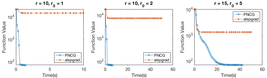
Figure 1: Comparison between PNCG and specialized solver alspgrad, showing the objective function value plotted against time. The algorithms are started near saddle points constructed as in (40).

6 Conclusion

In this article, we relate and compare different definitions of approximate second-order optimal point in literature and define our own for optimization with bounds. We proposed a projected Newton-CG method. It has good complexity guarantees and is designed with practicality in mind, and is related to the two-metric projection algorithms proposed in the 1980s. The projected Newton-CG terminates within $\mathcal{O}(\epsilon^{-3/2})$ iterations or $\tilde{\mathcal{O}}(\epsilon^{-7/4})$ number of Hessian-vector product/gradient evaluation operations and finds a point that is approximately second-order optimal to tolerance $\epsilon$, with high probability. Numerical experiments on nonnegative matrix factorization illustrate practicality of the methods.

In future work, we will consider extensions of the algorithms to solve optimization problems with more complex structures such as polyhedral feasible sets, $\ell_{1}$-norm terms, and even more general convex constraints that allow for cheap projection. We will also investigate complexity guarantees of the two-metric projection algorithm proposed by Bertsekas.

Appendix A Comparing approximate second-order optimality conditions

We show that the relation $\gtrsim$ is transitive.

Lemma 6

If $\text{\bf DefA}\gtrsim\text{\bf DefB}$ and $\text{\bf DefB}\gtrsim\text{\bf DefC}$, then $\text{\bf DefA}\gtrsim\text{\bf DefC}$.

Proof

Since $\text{\bf DefA}\gtrsim\text{\bf DefB}$, there exists $\epsilon_{A}\in(0,1]$ and $c_{A}>0$ such that for any $x\in\mathcal{X}$ and $\epsilon\in(0,\epsilon_{A}]$, if $x$ is an $(\epsilon,p)$-2o point by DefA, then $x$ is also a $(c_{A}\epsilon,p)$-2o point by DefB.

Likewise, since $\text{\bf DefB}\gtrsim\text{\bf DefC}$, there exists $\epsilon_{B}\in(0,1]$ and $c_{B}>0$ such that for any $x\in\mathcal{X}$ and $\epsilon\in(0,\epsilon_{B}]$, if $x$ is an $(\epsilon,p)$-2o point by DefB, then $x$ is also a $(c_{B}\epsilon,p)$-2o point by DefC.

Let $\bar{\epsilon}=\min\{\epsilon_{A},\epsilon_{B}/c_{A}\}$. Take arbitrary $x\in\mathcal{X}$ and $\epsilon\in(0,\bar{\epsilon}]$. Suppose that $x$ is an $(\epsilon,p)$-2o point by DefA. Since $\text{\bf DefA}\gtrsim\text{\bf DefB}$ and $\epsilon\leq\epsilon_{A}$, $x$ is a $(c_{A}\epsilon,p)$-2o point by DefB; Since $\text{\bf DefB}\gtrsim\text{\bf DefC}$ and $c_{A}\epsilon\leq\epsilon_{B}$, $x$ is also a $(c_{B}c_{A}\epsilon,p)$-2o point by DefC. Since the choice of $x\in\mathcal{X}$ and $\epsilon\in(0,\bar{\epsilon}]$ is arbitrary, we have that $\text{\bf DefA}\gtrsim\text{\bf DefC}$. ∎

We now give the proof of Theorem 3.2.

Proof

Let $U_{\mathcal{X}}\triangleq\max_{x\in\mathcal{X}}\|x\|_{\infty}$.

1. Suppose that $x$ is an $(\epsilon,p)$-2o point by Def2 and $\epsilon\leq 1$. We show (1) through the following steps.

   1. Fix any index $i$. Choose $d$ such that $d^{i}=\Delta$ and $d^{j}=0,\forall j\neq i$, then $\eqref{eq:em2o-cartis}\implies\nabla f(x)^{T}d=\nabla_{i}f(x)\Delta\geq-\Delta\epsilon\implies\nabla_{i}f(x)\geq-\epsilon$. This indicates that $\nabla f(x)\geq-\epsilon{\bf 1}.$

   2. Fix any index $i$. Let $d^{i}=-\mbox{sign}(\nabla_{i}f(x))\min\{\Delta,x^{i}\}$ and $d^{j}=0$, $\forall j\neq i$. Then $\eqref{eq:em2o-cartis}\implies\nabla f(x)^{T}d=-|\nabla_{i}f(x)|\min\{\Delta,x^{i}\}\geq-\Delta\epsilon\implies|\nabla_{i}f(x)|\leq\frac{\Delta\epsilon}{\min\{\Delta,x^{i}\}}$ $\implies|\nabla_{i}f(x)x^{i}|\leq\frac{\Delta x^{i}\epsilon}{\min\{\Delta,x^{i}\}}=\max\{x^{i},\Delta\}\epsilon\leq\max\{U_{\mathcal{X}},\Delta\}\epsilon.$ This indicates that $\|X\nabla f(x)\|_{\infty}$ $\leq\max\{U_{\mathcal{X}},\Delta\}\epsilon\leq\max\{U_{\mathcal{X}},\Delta_{\max}\}\epsilon.$

   3. If $x=0$, then second row of (13) holds trivially. Suppose that $x\neq 0$. Let $d\triangleq c_{d}Xv$, where $c_{d}\triangleq\min\left\{\frac{\Delta}{\|x\|_{\infty}},1\right\}$, $v$ is an arbitrary vector with $\|v\|_{2}=1$. Therefore, we have that $x+d\geq 0,x-d\geq 0,\|d\|\leq\Delta$. Therefore,

      $$-\Delta^{2}\epsilon^{p} \overset{\eqref{eq:em2o-cartis}}{\leq}\nabla f(x)^{T}d+\frac{1}{2}d^{T}\nabla^{2}f(x)d$$

      and also,

      $$-\Delta^{2}\epsilon^{p} \overset{\eqref{eq:em2o-cartis}}{\leq}-\nabla f(x)^{T}d+\frac{1}{2}d^{T}\nabla^{2}f(x)d.$$

      Therefore,

      $$-\Delta^{2}\epsilon^{p} \leq\frac{1}{2}d^{T}\nabla^{2}f(x)d=\frac{c_{d}^{2}}{2}v^{T}X\nabla^{2}f(x)Xv$$

      $$\implies v^{T}X\nabla^{2}f(x)Xv \geq-\frac{2\Delta^{2}}{c_{d}^{2}}\epsilon^{p}\geq-2\max\{\|x\|_{\infty}^{2},\Delta^{2}\}\epsilon^{p}\geq-2\max\{U_{\mathcal{X}}^{2},\Delta_{\max}^{2}\}\epsilon^{p}.$$

   Denote $c_{\Delta}\triangleq\left(2\max\{U_{\mathcal{X}}^{2},\Delta_{\max}^{2}\}\right)^{1/p}$. Therefore, by (1a)-(1c), $x$ is an $(c\epsilon,p)$-2o point by Def3, where $c\triangleq\max\{1,U_{\mathcal{X}},\Delta_{\max},c_{\Delta}\}$.

2. Given $x\geq 0$, let $T\triangleq\mathop{\hbox{\rm diag}}(t)$ be a diagonal matrix of $n\times n$ such that $t^{i}=1$ if $x^{i}\leq 1$ and $t^{i}=1/x^{i}$ if $x^{i}>1$. Then we have that $\bar{X}=XT=TX$.
   $\text{\bf Def3}\gtrsim\text{\bf Def4}$. Suppose that $x$ is an $(\epsilon,p)$-2o point by Def3. Note

   $$\|\bar{X}\nabla f(x)\|_{\infty}\leq\|X\nabla f(x)\|_{\infty}\leq\epsilon.$$

   $$d^{T}\bar{X}\nabla^{2}f(x)\bar{X}d=(Td)^{T}X\nabla^{2}f(x)XTd\geq-\epsilon^{p}\|Td\|^{2}\geq-\epsilon^{p}\|d\|^{2},\forall d\in\mathbb{R}^{n}.$$

   Therefore, $x$ is also an $(\epsilon,p)$-2o point by Def4.
   $\text{\bf Def4}\gtrsim\text{\bf Def3}$. $x$ is an $(\epsilon,p)$-2o point by Def4. Then

   $$\|X\nabla f(x)\|_{\infty}=\|T^{-1}\bar{X}\nabla f(x)\|_{\infty}\leq\|x\|_{\infty}\|\bar{X}\nabla f(x)\|_{\infty}\leq U_{\mathcal{X}}\epsilon.$$

   $$d^{T}X\nabla^{2}f(x)Xd=(T^{-1}d)^{T}\bar{X}\nabla^{2}f(x)\bar{X}(T^{-1}d)\geq-\epsilon^{p}\|T^{-1}d\|^{2}$$

   $$\geq-\epsilon^{p}\|x\|^{2}_{\infty}\|d\|^{2}\geq-(U_{\mathcal{X}}^{2/p}\epsilon)^{p}\|d\|^{2}.$$

   Then $x$ is also an $(\max\{U_{\mathcal{X}},U_{\mathcal{X}}^{2/p}\}\epsilon,p)$-2o point by Def3.

3. Obviously we have that $\text{\bf Def3}\gtrsim\text{\bf Def5}$. By (2) and the property of $\gtrsim$ and $\thickapprox$, $\text{\bf Def4}\gtrsim\text{\bf Def5}$.

4. Suppose that $x$ is an $(\epsilon,p)$-2o point by Def1. Let $J^{+}$, $J^{-}$, and $S$ be associated with $x$ as in Def1. Let $T=\mathop{\hbox{\rm diag}}(t)$ be a diagonal matrix of dimension $n\times n$ with $t^{i}=1$ for $i\in J^{+}$ and $t^{i}=x^{i}$, for $i\in J^{-}$. Then $X=TS$ and

   $$\|X\nabla f(x)\|_{\infty}\leq\|X\nabla f(x)\|=\|TS\nabla f(x)\|\leq\|T\|\|S\nabla f(x)\|$$

   $$\leq\max\{\|x\|_{\infty},1\}\|S\nabla f(x)\|\leq 2\max\{U_{\mathcal{X}},1\}\epsilon\leq\max\{U_{\mathcal{X}}^{2/p},2U_{\mathcal{X}},2\}\epsilon.$$

   Also, for any $d\in\mathbb{R}^{n}$, we have

   $$d^{T}X\nabla^{2}f(x)Xd=d^{T}TS\nabla^{2}f(x)STd\geq-\epsilon^{p}\|Td\|^{2}$$

   $$\geq-\epsilon^{p}\max\{\|x\|_{\infty}^{2},1\}\|d\|^{2}=-(\epsilon\max\{\|x\|_{\infty}^{2/p},1\})^{p}\|d\|^{2}$$

   $$\geq-(\epsilon\max\{U_{\mathcal{X}}^{2/p},1\})^{p}\|d\|^{2}\geq-(\epsilon\max\{U_{\mathcal{X}}^{2/p},2U_{\mathcal{X}},2\})^{p}\|d\|^{2}.$$

   If we let $c=\max\{U_{\mathcal{X}}^{2/p},2U_{\mathcal{X}},2\}$, then $x$ is an $(c\epsilon,p)$-2o point by Def5.

∎

The following example illustrates why Def2,Def3,Def4 are not essentially stronger than Def1.

Example 1

Consider problem (1),(2),(11) in 1-dimension. Let $f(x)=\frac{1}{4}x^{4}$ and $p\in(0,1]$. Given any $c>0$, there exists $\bar{\epsilon}\in(0,1)$ such that for any $\epsilon\in(0,\bar{\epsilon})$, we can find an $x\geq 0$ that is an $(\epsilon,p)$-2o point by Def2, Def3, Def4, but not a $(c\epsilon,p)$-2o point by Def1. In particular, choose $\bar{\epsilon}$ such that for any $\epsilon\in(0,\bar{\epsilon})$,

$$\epsilon^{7/24}\leq\Delta_{\max},\;\epsilon^{1/6}\leq\Delta_{\max},\;\epsilon^{1/6}\leq 6\Delta_{\max}^{2},\;\epsilon^{5/24}<c^{-1/2},\;\epsilon^{1/8}<\frac{1}{2c}.$$ (41)

Let $x=\epsilon^{7/24}$. Then $f^{\prime}(x)=x^{3}=\epsilon^{7/8},xf^{\prime}(x)=x^{4}=\epsilon^{7/6},f^{\prime\prime}(x)=3x^{2}\geq 0,\forall x\geq 0$. Apparently, $x$ is an $(\epsilon,p)$-2o point by Def3, Def4. Note that by (41),

$$\min_{x+d\geq 0,|d|\leq\Delta_{\max}}f^{\prime}(x)d=-x^{3}\cdot x=-\epsilon^{7/6}\geq-\Delta_{\max}\epsilon.$$

$$\min_{x+d\geq 0,|d|\leq\Delta_{\max}}f^{\prime}(x)d+\frac{1}{2}f^{\prime\prime}(x)d^{2}=\min_{x+d\geq 0,|d|\leq\Delta_{\max}}x^{3}d+\frac{3x^{2}}{2}\cdot d^{2}$$

$$\overset{(d^{*}=-x/3)}{=}-x^{4}/6=-\epsilon^{7/6}/6\geq-\Delta_{\max}^{2}\epsilon^{p}.$$

Therefore, $x$ is also an $(\epsilon,p)$-2o point by Def2(let $\Delta=\Delta_{\max}$). However, note that by (41),

$$x>\sqrt{c\epsilon}\implies J^{-}=\{1\};\;f^{\prime}(x)=\epsilon^{7/8}>2c\epsilon,$$

so $x$ is not an $(c\epsilon,p)$-2o point by Def1.

A definition of approximate second-order optimality proposed in nouiehed2020trust is adapted to the scope of our study by setting $\Omega=\mathbb{R}^{n}_{+}$, to obtain the following definition.

Definition 7 (nouiehed2020trust , Def7)

$x$ is an $(\epsilon,p)$-2o point of (1), (2), (11) according to Def7 if $x\in\Omega$, and

$$\begin{aligned} \left|\mbox{globalmin}_{x+d\in\Omega,\|d\|\leq 1}\quad\nabla f(x)^{T}d\right|&\leq\epsilon,\\ \left|\mbox{globalmin}_{x+d\in\Omega,\|d\|\leq 1,\nabla f(x)^{T}d\leq 0}\quad d^{T}\nabla^{2}f(x)d\right|&\leq\epsilon^{p}.\end{aligned}$$ (42)

The next result states that Def2 is essentially stronger than Def7, which in turn is essentially stronger than Def3.

Theorem A.1

(1). $\text{\bf Def2}\gtrsim\text{\bf Def7}$; (2). $\text{\bf Def7}\gtrsim\text{\bf Def3}$.

Proof

• Suppose that $x$ is an $(\epsilon,p)$-2o point by Def2. Let $d_{1}^{*}$ and $d_{2}^{*}$ be the solution of the first and second problems in (42), respectively. WLOG, suppose that $\|d_{1}^{*}\|\neq 0$, $\|d_{2}^{*}\|\neq 0$. Define $\bar{d_{i}}=d_{i}^{*}\min\{\Delta/\|d_{i}^{*}\|,1\}$, $i=1,2$. Then $\bar{d}_{1}$ and $\bar{d}_{2}$ are feasible points in (12). Then we have

  $$\nabla f(x)^{T}\bar{d}_{1} \geq-\Delta\epsilon,$$

  $$\implies\nabla f(x)^{T}d_{1}^{*} =\nabla f(x)^{T}\bar{d}_{1}\max\{\|d_{1}^{*}\|/\Delta,1\}$$

  $$\geq-\Delta\max\{\|d_{1}^{*}\|/\Delta,1\}\epsilon=-\max\{\|d_{1}^{*}\|,\Delta\}\epsilon\geq-\max\{\Delta_{\max},1\}\epsilon.$$

  Moreover, we have

  $$\frac{1}{2}\bar{d}_{2}^{T}\nabla^{2}f(x)\bar{d}_{2}+\nabla f(x)^{T}\bar{d}_{2}\geq-\Delta^{2}\epsilon^{p},$$

  which implies that

  $$\frac{1}{2}\bar{d}_{2}^{T}\nabla^{2}f(x)\bar{d}_{2}\geq-\Delta^{2}\epsilon^{p},$$

  since $\nabla f(x)^{T}\bar{d}_{2}\leq 0$. Therefore, we have

  $$\frac{1}{2}(d_{2}^{*})^{T}\nabla^{2}f(x)d_{2}^{*}=\frac{1}{2}\bar{d}_{2}^{T}\nabla^{2}f(x)\bar{d}_{2}(\max\{\|d_{2}^{*}\|/\Delta,1\})^{2}\geq-\Delta^{2}(\max\{\|d_{2}^{*}\|/\Delta,1\})^{2}\epsilon^{p}$$

  $$=-\max\{\|d_{2}^{*}\|^{2},\Delta^{2}\}\epsilon^{p}\geq-\max\{\Delta_{\max}^{2},1\}\epsilon^{p}.$$

  Altogether, these expressions imply that $x$ is an $(c\epsilon,p)$-2o point by Def7 where
  $c=\max\{2^{1/p}\Delta_{\max}^{2/p},\Delta_{\max},2^{1/p}\}$.

• Let $U_{\mathcal{X}}\triangleq\max_{x\in\mathcal{X}}\|x\|_{\infty}$. Suppose that $x$ is an $(\epsilon,p)$-2o point by Def7. Similar to the proof of Theorem 3.2, first row of (13) holds because $\nabla f(x)\geq-\epsilon{\bf 1}$, and $\|X\nabla f(x)\|_{\infty}\leq\max\{U_{\mathcal{X}},1\}\epsilon$. Consider now the second row of (13). If $x=0$, this condition holds trivially. When $x\neq 0$, let $d\triangleq c_{d}Xv$, where $c_{d}\triangleq\min\left\{\frac{1}{\|x\|_{\infty}},1\right\}$, $v$ is an arbitrary vector with $\|v\|_{2}=1$. Let $\bar{d}=-{\rm sign}(\nabla f(x)^{T}d)d$. Therefore, we have that $x+\bar{d}\geq 0,\|\bar{d}\|\leq 1$, $\nabla f(x)^{T}\bar{d}\leq 0$. According to Def7, we have

  $$\bar{d}^{T}\nabla^{2}f(x)\bar{d}\geq-\epsilon^{p}$$

  Therefore,

  $$-\epsilon^{p} \leq\bar{d}^{T}\nabla^{2}f(x)\bar{d}=d^{T}\nabla^{2}f(x)d=c_{d}^{2}v^{T}X\nabla^{2}f(x)Xv$$

  $$\implies v^{T}X\nabla^{2}f(x)Xv \geq-\epsilon^{p}/c_{d}^{2}\geq-\max\{\|x\|_{\infty}^{2},1\}\epsilon^{p}\geq-\max\{U_{\mathcal{X}}^{2},1\}\epsilon^{p}.$$

  Altogether, $x$ is an $(c\epsilon,p)$-2o point by Def3, where $c=\max\{U_{\mathcal{X}}^{2/p},U_{\mathcal{X}},1\}$.

Appendix B Capped conjugate gradient algorithm

The version of the conjugate gradient method shown in Algorithm 3 was described in (Royer2019, , Algorithm 1) to solve a system of the form $\bar{H}y=-g$, where $\bar{H}=H+2\epsilon I$ is a damped version of the symmetric matrix $H$, which in our case is a principal submatrix of the Hessian $\nabla^{2}f(x_{k})$. Note that the following results hold regarding Algorithm 3, as is shown in (Royer2019, , Lemma 3) and (Royer2019, , Lemma 1).

Lemma 7

Consider the inputs $H,g,\epsilon$ and outputs d_type and $d$ of Algorithm 3, if
1. d_type=SOL, then

$$d^{T}(H+2\epsilon I)d\geq\epsilon\|d\|^{2},\quad\|d\|\leq 1.1\epsilon^{-1}\|g\|,\quad\|r\|\leq\frac{1}{2}\epsilon\zeta\|d\|,$$

where $r\triangleq(H+2\epsilon I)d+g$.
2. d_type = NC and $\bar{d}\triangleq-\mathop{\hbox{\rm sgn}}(d^{T}g)\frac{d^{T}Hd}{\|d\|^{2}}\frac{d}{\|d\|}$, then $\bar{d}^{T}g\leq 0$ and

$$\frac{\bar{d}^{T}H\bar{d}}{\|\bar{d}\|^{2}}=-\|\bar{d}\|\leq-\epsilon.$$

Lemma 8

Number of matrix-vector multiplication of Algorithm 3 is bounded by

$$2\min\{n,\mathbb{J}(M,\epsilon,\zeta)\}+1,$$

where

$$\mathbb{J}(M,\epsilon,\zeta)\leq\min\left\{n,\left\lceil\left(\sqrt{\kappa}+\frac{1}{2}\right)\log\left(\frac{144(\sqrt{\kappa}+1)^{2}\kappa^{6}}{\zeta^{2}}\right)\right\rceil\right\}.$$

Algorithm 3 Capped Conjugate Gradient

  Inputs: Symmetric matrix $H\in\mathbb{R}^{n\times n}$; vector $g\neq 0$; damping parameter $\epsilon\in(0,1)$; desired relative accuracy $\zeta\in(0,1)$;

  Optional input: scalar $M$ (set to $0$ if not provided);

  Outputs: d_type, $d$;

  Secondary outputs: final values of $M$, $\kappa$, $\hat{\zeta}$, $\tau$, and $T$;

  Set

$$\bar{H}:=H+2\epsilon I,\quad\kappa:=\frac{M+2\epsilon}{\epsilon},\quad\hat{\zeta}:=\frac{\zeta}{3\kappa},\quad\tau:=\frac{\sqrt{\kappa}}{\sqrt{\kappa}+1},\quad T:=\frac{4\kappa^{4}}{(1-\sqrt{\tau})^{2}};$$

  Set $y_{0}\leftarrow 0$, $r_{0}\leftarrow g$, $p_{0}\leftarrow-g$, $j\leftarrow 0$;

  if $p_{0}^{\top}\bar{H}p_{0}<\epsilon\|p_{0}\|^{2}$ then

     Set $d=p_{0}$ and terminate with d_type=NC;

  else if $\|Hp_{0}\|>M\|p_{0}\|$ then

     Set $M\leftarrow{\|Hp_{0}\|}/{\|p_{0}\|}$ and update $\kappa,\hat{\zeta},\tau,T$ accordingly;

  end if

  while TRUE do

     $\alpha_{j}\leftarrow{r_{j}^{\top}r_{j}}/{p_{j}^{\top}\bar{H}p_{j}}$; {Begin Standard CG Operations}

     $y_{j+1}\leftarrow y_{j}+\alpha_{j}p_{j}$;

     $r_{j+1}\leftarrow r_{j}+\alpha_{j}\bar{H}p_{j}$;

     $\beta_{j+1}\leftarrow{(r_{j+1}^{\top}r_{j+1})}/{(r_{j}^{\top}r_{j})}$;

     $p_{j+1}\leftarrow-r_{j+1}+\beta_{j+1}p_{j}$; {End Standard CG Operations}

     $j\leftarrow j+1$;

     if $M<\max\left(\|Hp_{j}\|/\|p_{j}\|,\|Hy_{j}\|/\|y_{j}\|,\|Hr_{j}\|/\|r_{j}\|\right)$ then

        Set $M\leftarrow\max\left(\|Hp_{j}\|/\|p_{j}\|,\|Hy_{j}\|/\|y_{j}\|,\|Hr_{j}\|/\|r_{j}\|\right)$ and update $\kappa,\hat{\zeta},\tau,T$ accordingly;

     end if

     if $y_{j}^{\top}\bar{H}y_{j}<\epsilon\|y_{j}\|^{2}$ then

        Set $d\leftarrow y_{j}$ and terminate with d_type=NC;

     else if $\|r_{j}\|\leq\hat{\zeta}\|r_{0}\|$ then

        Set $d\leftarrow y_{j}$ and terminate with d_type=SOL;

     else if $p_{j}^{\top}\bar{H}p_{j}<\epsilon\|p_{j}\|^{2}$ then

        Set $d\leftarrow p_{j}$ and terminate with d_type=NC;

     else if $\|r_{j}\|>\sqrt{T}\tau^{j/2}\|r_{0}\|$  then

        Compute $\alpha_{j},y_{j+1}$ as in the main loop above;

        Find $i\in\{0,\dotsc,j-1\}$ such that

$$\frac{(y_{j+1}-y_{i})^{\top}\bar{H}(y_{j+1}-y_{i})}{\|y_{j+1}-y_{i}\|^{2}}\;<\;\epsilon;$$ (43)

        Set $d\leftarrow y_{j+1}-y_{i}$ and terminate with d_type=NC;

     end if

  end while

Appendix C Minimum eigenvalue oracle (MEO) procedure

The procedure shown as Procedure 4 is used to identify a direction of significant negative curvature, smaller than a threshold $-\epsilon/2$ for a given $\epsilon>0$, or else return a certificate that all eigenvalues of $H$ are greater than $-\epsilon$. In the latter case, the certificate may be wrong, with probability up to a supplied tolerance $\delta$. This procedure is defined in (Royer2019, , Procedure 2), where a discussion of various possible implementations is given. The most interesting implementation for our purposes is a randomized Lanczos procedure, which performs a single matrix-vector product involving $H$ at each of its iterations, and which finds the minimum eigenvalue of the projection of $H$ onto a Krylov subspace seeded by an initial random vector at each iteration.

Procedure 4 Minimum Eigenvalue Oracle (MEO)

  Inputs: Symmetric matrix $H\in\mathbb{R}^{n\times n}$, tolerance $\epsilon>0$, error probability $\delta\in[0,1)$;

  Optional input: Upper bound on Hessian norm $M$;

  Outputs: An estimate $\lambda$ of $\lambda_{\min}(H)$ such that $\lambda\leq-\epsilon/2$, and vector $v$ with $\|v\|=1$ such that $v^{\top}Hv=\lambda$ OR a certificate that $\lambda_{\min}(H)\geq-\epsilon$. The probability that the certificate is issued but $\lambda_{\min}(H)<-\epsilon$ is at most $\delta$.

Based on the discussion in (Royer2019, , Section 3.2) and (Royer2019, , Assumption 3), we have the following result about bound on Hessian-vector products when a randomized Lanczos procedure (or a randomized CG) is used to implement Procedure 4.

Lemma 9

We use a randomized Lanczos method with a starting vector uniformly generated on a unit sphere to implement Procedure 4. Then given a failure probability $0<\delta\ll 1$, Procedure 4 either certifies that $H\succeq-\epsilon I$ or finds a direction along which curvature of $H$ is smaller than $-\epsilon/2$ in at most $N^{\mbox{\rm\scriptsize meo}}\triangleq\min\{n,1+\lceil\mathcal{C}^{\mbox{\rm\scriptsize meo}}\epsilon^{-1/2}\rceil\}$ Hessian-vector products, where $\mathcal{C}^{\mbox{\rm\scriptsize meo}}=\log(2.75n/\delta^{2})\sqrt{\|H\|\max\{1,\epsilon^{2}\}}/2.$ If $\lambda_{\min}(H)<-\epsilon$, then with probability at most $\delta$, a certificate will be given.

Appendix D Two-sided bounds

In this section we consider the two-sided bound-constrained optimization:

$$\min\,f(x)\quad\mbox{s.t.}\;\;x\in\Omega\triangleq\{x\in\mathbb{R}^{n}\mid 0\leq x^{i}\leq u^{i},\;i\in\mathcal{I}\}$$ (44)

where $f:\mathbb{R}^{n}\rightarrow\mathbb{R}$ is twice continuously differentiable and is bounded below by $f_{\rm low}$ on the feasible region $\Omega$, and $\mathcal{I}\subset\{1,2,\dotsc,n\}$. We assume without loss of generality that $u^{i}>0$ for all $i\in\mathcal{I}$. We allow $u_{i}=\infty$, that is, not all components $x_{i}$ for $i\in\mathcal{I}$ have upper bounds.

Extending Definition 1, we define approximate optimality for (44) as follows.

Definition 8 ($(\epsilon,p)$-2o of (44))

We say that $x$ is an $(\epsilon,p)$-2o point for (44) if and only if

$$0\leq x^{i}\leq u^{i},\;i\in\mathcal{I},\;\|S\nabla f(x)\|\leq 2\epsilon,\mbox{ and }\begin{cases}\nabla_{i}f(x)\geq-\epsilon^{3/4},&\;i\in\mathcal{I},x_{k}^{i}\leq\sqrt{\epsilon},\\ \nabla_{i}f(x)\leq\epsilon^{3/4},&\;i\in\mathcal{I},x_{k}^{i}\geq u^{i}-\sqrt{\epsilon},\end{cases}$$

$$S\nabla^{2}f(x)S\succeq-\epsilon^{p}I,$$

where we define $J^{+}\triangleq\{i\in\mathcal{I}\mid 0\leq x^{i}\leq\sqrt{\epsilon}\mbox{ or }u^{i}-\sqrt{\epsilon}\leq x^{i}\leq u^{i}\}$, $J^{-}\triangleq\{1,\ldots,n\}\setminus J^{+}$, $S=\mathop{\hbox{\rm diag}}({s})$, where $s^{i}=\min\{x^{i},u^{i}-x^{i}\}$ if $i\in J^{+}$, and $s^{i}=1$ if $i\in J^{-}$. Again, this definition reduces to Definition 1 when $u^{i}=+\infty$ for all $i\in\mathcal{I}$, and can be motivated by exact (weak) second-order optimal conditions of (44). The extension of projected Newton-CG (Algorithm 1) to the general bound-constrained optimization (44) is relatively straightforward. We redefine the projection operator $P$, index sets $J_{k}^{+}$ and $J_{k}^{-}$, and $S_{k}=\mathop{\hbox{\rm diag}}(s_{k})$ as follows:

$$[P(x)]^{i} \triangleq\begin{cases}\mbox{mid}(0,x^{i},u^{i})&\;i\in\mathcal{I},\\ x^{i}&\;\mbox{otherwise},\end{cases}$$

$$J_{k}^{+} \triangleq\{i\in\mathcal{I}\mid 0\leq x_{k}^{i}\leq\epsilon_{k}\mbox{ or }u^{i}-\epsilon_{k}\leq x_{k}^{i}\leq u^{i}\},$$

$$J_{k}^{-} \triangleq\{1,\ldots,n\}\setminus J_{k}^{+}=\{i\in\mathcal{I}\mid\epsilon_{k}<x_{k}^{i}<u^{i}-\epsilon_{k}\}\cup\mathcal{I}^{c}.$$

$$s_{k}^{i} =\begin{cases}\min\{x_{k}^{i},u^{i}-x_{k}^{i}\},&\mbox{if }i\in J_{k}^{+},\\ 1,&\mbox{otherwise.}\end{cases}$$

The definitions of $g^{-}_{k}$, $H^{-}_{k}$, $g^{+}_{k}$ and $S^{+}_{k}$, are the same, modulo the redefined $P$, $J_{k}^{+}$, $J_{k}^{-}$, and $S_{k}$. For Algorithm 1, the only adjustment to be made is the conditions to trigger the gradient step, which become

$$g_{k}^{i}<-\epsilon_{k}^{3/2},x_{k}^{i}\leq\epsilon_{k},i\in\mathcal{I}\mbox{ or }g_{k}^{i}>\epsilon_{k}^{3/2},x_{k}^{i}\geq u^{i}-\epsilon_{k},i\in\mathcal{I}\mbox{ or }\|S^{+}_{k}g^{+}_{k}\|\geq\epsilon_{k}^{2}.$$

We make an additional assumption on $\epsilon_{k}$ that

$$2\epsilon_{k}\leq u^{i},\quad\forall k\geq 0,\ i\in\mathcal{I},$$

and assume that Assumption 1 and 2 hold when $\Omega$ includes two-sided bounds. It can then be verified that Lemmas 3, 4 and 5 still hold for the modified Algorithm 1. Lemma 2 also holds if the conditions to trigger the gradient step is tailored accordingly. Furthermore, if we let $\epsilon_{k}\equiv\epsilon_{H}=\sqrt{\epsilon}$ and $\epsilon_{g}=\epsilon$, then the Algorithm stops within the same number of iterations specified in Theorem 4.1 ($\mathcal{O}(\epsilon^{-3/2})$) and locates an $x$ that is an $(\epsilon,1/2)$-2o point of (44) with probability at least $(1-\delta)^{K_{\mbox{\rm\scriptsize pncg}}}$, where $\delta\in[0,1)$ is the probability of failure in Procedure 4. Moreover, the complexity of fundamental operations (gradient evaluations or Hessian-vector products) is also $\tilde{O}(\epsilon^{-7/4})$.

References

- (1) Bertsekas, D.P.: Projected Newton methods for optimization problems with simple constraints. SIAM Journal on Control and Optimization 20(2), 221–246 (1982). DOI 10.1137/0320018
- (2) Bertsekas, D.P.: Constrained optimization and Lagrange multiplier methods. Academic Press (2014)
- (3) Bertsekas, D.P.: Nonlinear Programming, third edn. Athena Scientific, Belmont, MA 02478 (2016)
- (4) Bian, W., Chen, X., Ye, Y.: Complexity analysis of interior point algorithms for non-Lipschitz and nonconvex minimization. Mathematical Programming 149(1), 301–327 (2015). DOI 10.1007/s10107-014-0753-5
- (5) Birgin, E.G., Martínez, J.M.: Complexity and performance of an augmented lagrangian algorithm. Optimization Methods and Software 35(5), 885–920 (2020)
- (6) Birgin, E.G., Martínez, J.M.: On regularization and active-set methods with complexity for constrained optimization. SIAM Journal on Optimization 28(2), 1367–1395 (2018)
- (7) Cartis, C., Gould, N.I., Toint, P.L.: Universal regularization methods: varying the power, the smoothness and the accuracy. SIAM Journal on Optimization 29(1), 595–615 (2019)
- (8) Cartis, C., Gould, N.I.M., Toint, P.L.: An adaptive cubic regularization algorithm for nonconvex optimization with convex constraints and its function-evaluation complexity. IMA Journal of Numerical Analysis 32(4), 1662–1695 (2012)
- (9) Cartis, C., Gould, N.I.M., Toint, P.L.: On the evaluation complexity of constrained nonlinear least-squares and general constrained nonlinear optimization using second-order methods. SIAM Journal on Numerical Analysis 53(2), 836–851 (2015)
- (10) Cartis, C., Gould, N.I.M., Toint, P.L.: Second-order optimality and beyond: Characterization and evaluation complexity in convexly constrained nonlinear optimization. Foundations of Computational Mathematics 18(5), 1073–1107 (2018)
- (11) Chen, X., Toint, P.L., Wang, H.: Partially separable convexly-constrained optimization with non-Lipschitzian singularities and its complexity. arXiv preprint arXiv:1704.06919 (2017)
- (12) Curtis, F.E., Robinson, D.P., Samadi, M.: Complexity analysis of a trust funnel algorithm for equality constrained optimization. SIAM Journal on Optimization 28(2), 1533–1563 (2018)
- (13) Dvurechensky, P., Staudigl, M.: Hessian barrier algorithms for non-convex conic optimization. arXiv preprint arXiv:2111.00100 (2021)
- (14) Ghadimi, S., Lan, G., Zhang, H.: Mini-batch stochastic approximation methods for nonconvex stochastic composite optimization. Mathematical Programming 155(1), 267–305 (2016)
- (15) Gillis, N.: The why and how of nonnegative matrix factorization. In: J.A.K. Suykens, M. Signoretto, A. Argyriou (eds.) Regularization, Optimization, Kernels, and Support Vector Machines, Machine Learning and Pattern Recognition, pp. 257–291. Chapman & Hall/CRC (2014)
- (16) Gong, P., Zhang, C.: Efficient nonnegative matrix factorization via projected Newton method. Pattern Recognition 45(9), 3557–3565 (2012)
- (17) Grapiglia, G.N., Yuan, Y.X.: On the complexity of an augmented lagrangian method for nonconvex optimization. IMA Journal of Numerical Analysis 41(2), 1546–1568 (2021)
- (18) Griewank, A., Walther, A.: Evaluating derivatives: principles and techniques of algorithmic differentiation. SIAM (2008)
- (19) Haeser, G., Liu, H., Ye, Y.: Optimality condition and complexity analysis for linearly-constrained optimization without differentiability on the boundary. Mathematical Programming (2018). DOI 10.1007/s10107-018-1290-4
- (20) Kim, J., Park, H.: Toward faster nonnegative matrix factorization: A new algorithm and comparisons. In: 2008 Eighth IEEE International Conference on Data Mining, pp. 353–362. IEEE (2008)
- (21) Lin, C.J.: Projected gradient methods for nonnegative matrix factorization. Neural computation 19(10), 2756–2779 (2007)
- (22) Lin, Q., Ma, R., Xu, Y.: Complexity of an inexact proximal-point penalty method for constrained smooth non-convex optimization. Computational Optimization and Applications pp. 1–50 (2022)
- (23) Moré, J.J., Toraldo, G.: On the solution of large quadratic programming problems with bound constraints. SIAM Journal on Optimization 1(1), 93–113 (1991). DOI 10.1137/0801008. URL https://doi.org/10.1137/0801008
- (24) Nocedal, J., Wright, S.J.: Numerical Optimization, second edn. Springer Science & Business Media (2006)
- (25) Nouiehed, M., Razaviyayn, M.: A trust region method for finding second-order stationarity in linearly constrained nonconvex optimization. SIAM Journal on Optimization 30(3), 2501–2529 (2020)
- (26) O’Neill, M., Wright, S.J.: A log-barrier Newton-CG method for bound constrained optimization with complexity guarantees. IMA Journal of Numerical Analysis (2020). DOI 10.1093/imanum/drz074
- (27) Royer, C.W., O’Neill, M., Wright, S.J.: A Newton-CG algorithm with complexity guarantees for smooth unconstrained optimization. Mathematical Programming (2019). DOI 10.1007/s10107-019-01362-7
- (28) Royer, C.W., Wright, S.J.: Complexity analysis of second-order line-search algorithms for smooth nonconvex optimization. SIAM Journal on Optimization 28(2), 1448–1477 (2018). DOI 10.1137/17M1134329
- (29) Sahin, M.F., Alacaoglu, A., Latorre, F., Cevher, V., et al.: An inexact augmented Lagrangian framework for nonconvex optimization with nonlinear constraints. Advances in Neural Information Processing Systems 32 (2019)
- (30) Xie, Y., Wright, S.J.: Complexity of proximal augmented Lagrangian for nonconvex optimization with nonlinear equality constraints. Journal of Scientific Computing 86(3), 1–30 (2021)