Tasting the cake: evaluating self-supervised generalization on out-of-distribution multimodal MRI data

Abstract

Self-supervised learning has enabled significant improvements on natural image benchmarks. However, there is less work in the medical imaging domain in this area. The optimal models have not yet been determined among the various options. Moreover, little work has evaluated the current applicability limits of novel self-supervised methods. In this paper, we evaluate a range of current contrastive self-supervised methods on out-of-distribution generalization in order to evaluate their applicability to medical imaging. We show that self-supervised models are not as robust as expected based on their results in natural imaging benchmarks and can be outperformed by supervised learning with dropout. We also show that this behavior can be countered with extensive augmentation. Our results highlight the need for out-of-distribution generalization standards and benchmarks to adopt the self-supervised methods in the medical imaging community.

1 Introduction

Self-supervised learning has fueled recent advances in image recognition (Oord et al., 2018; Hjelm et al., 2018; Bachman et al., 2019; Tian et al., 2019; Chen et al., 2020; Grill et al., 2020; Chen & He, 2020) and spurred great interest and high expectations in neuroimaging (Fedorov et al., 2019; Mahmood et al., 2020; Jeon et al., 2020; Taleb et al., 2020; Fedorov et al., 2020b). The expectations are generally high even outside neuroimaging, so much so that in Yann LeCun’s metaphor of learning as a cake (LeCun, 2019), self-supervised learning makes the tastiest part of the cake: the filling.

However, the observed similarity in performance of self-supervised and supervised methods on natural images (Geirhos et al., 2020b) does not guarantee the same for other domains. Work on the generalization of these methods in neuroimaging data is generally lacking. We investigate the out-of-distribution generalization using simulated distortions and a natural distributional shift based on race with multimodal human MRI data to fill this gap. The multimodal data is as a natural case of multi-view data. It contains a wealth of complementary information regarding the healthy and dysfunctional brain (Calhoun & Sui, 2016). We show that on neuroimaging data, contrastive multimodal self-supervised learning leads to models that differ from models trained in a supervised way. The models disagree in how they react to distortions or modality. When using Dropout (Tompson et al., 2015), supervised models, counter to our expectations, can significantly outperform self-supervised models in out-of-distribution generalization. Further, the class of methods inspired by DeepInfoMax (DIM) (Hjelm et al., 2018) tends to struggle with intensity-based distortions, which we attempt to solve using additional data augmentation. Our findings further reinforce the advantages of multimodal models over unimodal ones.

Finally, we argue that the medical imaging community needs standards and benchmarks for out-of-distribution generalization. Introducing them could advance researchers towards a more reliable and standardized evaluation of newly proposed methods because similar performance on downstream tasks does not necessarily imply robust generalization. Standards could lead to a better understanding of methodological trade-offs in medical imaging. For example, the out-of-distribution generalization to distortions (e.g., affine scale distortion) may drive models to learn trivial discriminative features (see shortcut (Geirhos et al., 2020a)).

2 Methodology

2.1 Dataset and modeling out-of-distribution generalization

We evaluate the model on multimodal neuroimaging dataset OASIS-3 (LaMontagne et al., 2019). The modalities we selected are T1 and resting-state fMRI (rs-fMRI), which capture the brain’s anatomy and functional dynamics, respectively. First, T1 volumes were masked to only include the brain, and the rs-fMRI volumes were used to compute the fractional amplitude of low-frequency fluctuation (fALFF) in the $0.01$ to $0.1$Hz power band. The exhaustive details can be found in Appendix A.2.

To model out-of-distribution data, we utilize the following random data transformations available in TorchIO (Pérez-García et al., 2020): Affine, Elastic, Gamma, Motion, Spike, Ghosting, BiasField, GaussianNoise. The transformation details can be found in Appendix A.1. The samples are shown in the Appendix in Figure 4. To model natural distributional shift from the training set, we selected African-American subjects.

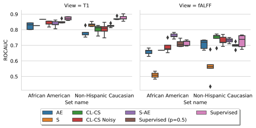
Figure 1: Left: The combined scheme of CL–CS and S–AE. Red arrow defines CS, Pink — CL, Purple — S, and Green — reconstruction for AE. Decoder $D$ is only required for S–AE, as CL–CS is a decoder-free model. Right: ROCAUC for holdout test sets with Non-Hispanic Caucausian and African American subjects for T1 and fALFF.

2.2 Multimodal self-supervised models

Let ${\cal D}=\{x^{\text{T1}}_{i},x^{\text{fALFF}}_{i}\}_{i=1}^{N}$ be a dataset with $N$ paired T1 and fALFF volumes. We want to learn a latent representation $z^{M}=E^{M}_{\theta_{M}}(x^{M})\in\mathbb{R}^{64}$ where $E^{m}_{\theta_{m}}$ is an encoder part of the 3D convolutional DCGAN architecture (Radford et al., 2015) for modality $M$.

Based on the performance of the proposed taxonomy in Fedorov et al. (2020a), we selected the following multimodal self-supervised models: CL–CS (Cross-Local and Cross-Spatial connections) and S–AE (Similarity AutoEncoder) (Figure 1). Additionally, we compare these models with Supervised (pretraining with cross-entropy) and AutoEncoder (AE) unimodal models, and multimodal models based only on the maximization of similarity (S) between latent representations. The model S is equivalent to SimCLR (Chen et al., 2020).

CL–CS is an AMDIM (Bachman et al., 2019) inspired model. Its inductive bias is to maximize mutual information between a p‘air of global and local variables. The first part of the objective, called CL, is defined between a ”local” variable $c$ (embedding of the location in the convolutional featuremap) in layer $l$ and a ”global” (latent) variable $z$ as $\{(c_{j,l}^{M},z^{L})_{M\neq L}\}$, where $j$ is the location index, and $M$ and $L$ are modality indexes. The second part of the objective, called CS, is defined on pairs $\{(c_{j,l}^{M},c_{k,l}^{L})_{M\neq L}\}$ where $k$ is a location index in the other modality. The CL–CS objective is by minimizing ${\cal L}_{\text{CL--CS}}=I_{\text{CL}}(\{c\}_{\text{T1}};\{z\}_{\text{fALFF}})+I_{\text{CL}}(\{c\}_{\text{fALFF}};\{z\}_{\text{T1}})+I_{\text{CS}}(\{c\}_{\text{T1}};\{c\}_{\text{fALFF}})+I_{\text{CS}}(\{c\}_{\text{fALFF}};\{c\}_{\text{T1}})$, where $I(\{u\}_{M};\{v\}_{L})=-\frac{1}{N}\sum_{n=1}^{N}\log\frac{e^{f(u^{M}_{n},v^{L}_{n})}}{\frac{1}{N}\sum_{k=1}^{N}e^{f(u_{n}^{M},v_{k}^{L})}}$ is an InfoNCE (Oord et al., 2018) based estimator with a separable critic $f(u^{M}_{n},v^{L}_{k})=\frac{u^{M\intercal}_{n}v^{L}_{k}}{\sqrt{n}}$ (Bachman et al., 2019) and $n=64$ is the dimensionality of the embeddings.

S–AE is a fusion of CMC (Tian et al., 2019) and SimCLR (Chen et al., 2020) with DCCAE (Wang et al., 2015), where the CCA objective is substituted by a maximization of similarity (mutual information) between a pair of latent variables $\{(z^{M},z^{L})_{M\neq L}\}$. The similarity is approximated with a DIM objective that allows the model to be trained end-to-end and improves numerical stability compared to SVD-based solutions of CCA (Wang et al., 2015). Combining an AE with similarity maximization is shown to avoid the collapse of its representation in a multimodal scenario (Fedorov et al., 2020a). The S–AE objective is by minimizing ${\cal L}_{\text{S--AE}}=I(\{z\}_{\text{T1}};\{z\}_{\text{fALFF}})+I(\{z\}_{\text{fALFF}};\{z\}_{\text{T1}})+R^{\text{T1}}+R^{\text{fALFF}}$, where $R^{M}=\frac{1}{N}\sum_{n=1}^{N}||x^{M}_{n}-D^{M}(E^{M}(x^{M}_{n}))||^{2}$ is a reconstruction loss with a DCGAN decoder $D$ for modality $M$.

3 Results and Discussion

In our experiments, we use the frozen encoder and linear projection trained on Non-Hispanic Caucasian subjects. First, we pretrain the encoder on all possible pairs; then, we train a linear projection from the encoder’s output to classify Healthy Controls (HC) and patients with Alzheimer’s Disease (AD). Eventually, we evaluate the out-of-distribution generalization on a natural race-based distributional shift and simulated distortions applied to volumes in standardized MNI space. All the models follow the same pipeline and use the same hyperparameters (Appendix A.3).

Figure 2: ROCAUC performance for out-of-distribution generalization on T1 data with simulated distortions. Each title contains the name of a random distorsion and x-axis label — parameter of the distorsion.

3.1 Do self-supervised multimodal models produce robust representations?

In Figure 2 we compare the results of selected models and their baselines on out-of-distributional generalization with simulated distortions. In most cases, the supervised model performs quite well and better than the self-supervised models, except it may break down on RandomGhosting, RandomSpike, RandomBlur, and Random Noise for stronger distortion levels. The unimodal AE and multimodal S perform much worse compared to the combined approach: S–AE. CL–CS performs much worse than other models on intensity-based noise: RandomGhosting, RandomSpike, RandomBlur, RandomNoise. We hypothesize that adding intensity-based data-augmentation should help DIM-inspired models. DIM-inspired models maximize the mutual information between features with respect to depth, which can lead to learning spurious correlations.

In Figure 3 we compare models on out-of-distributional performance for fALFF. Specifically, in this case, S completely fails to represent fALFF, and the unimodal AE may fail in most cases. The multimodal self-supervised models: S–AE and CL–CS outperform the supervised baseline in most cases.

We want to note that fALFF is a ”harder” modality because it represents rs-fMRI as a timeless and less-informative voxel-wise hand-engineered feature. Visually (Figure 1 (left)), it looks highly noisy compared to T1. Importantly, most of the distortions used to augment the data are not natural variations in the fALFF data because it has undergone a heavy preprocessing pipeline.

It is unclear what generalization requirements we should satisfy in medical imaging and what out-of-distribution generalization is meaningful. For example, if we look at the first subfigure with the RandomAffine and scale parameter in Figure 2, it is not clear whether generalization to scaling is desirable. When we scale the volume 1.7$\times$ or more, we can only see the center of the brain, which might force some models (Supervised, CL–CS) to learn trivial features, such as a reduced ventricle size is a well-known trivial biomarker for Alzheimer’s disease (Frisoni et al., 2010). In contrast, other models (AE, S, S–AE) try to utilize information from the whole brain for decision making because they aren’t directly optimizing an objective that maximizes classification accuracy.

Figure 3: ROCAUC performance for out-of-distribution generalization on fALFF data with simulated distortions. Each title contains the name of a random distorsion and x-axis label — parameter of the distorsion.

These findings suggest contrastive multimodal self-supervised learning produces models that differ strongly from models trained in a supervised way but that there is room for improvement for both methods. We explore the improvement of Supervised and DIM models in the next subsection.

3.1.1 Improving out-of-distribution generalization of supervised and DIM inspired models

To improve the supervised model’s out-of-distribution generalization, we utilized volumetric (3D) Dropout with $p=0.5$. The Supervised model with dropout shows a significant boost in generalization for T1 volumes compared to self-supervised models (Supervised (p=0.5), Figure 2). Additionally, dropout did push the model to not only extract features from the center of the brain Figure 2 for RandomAffine scale distortion. This may suggest that dropout is a simple solution to the problem. Dropout however, does not work for noisy and hand-engineered fALFF data (Figure 3).

To improve the out-of-distribution generalization for CL–CS, we added RandomNoise with a maximum standard deviation of $1.0$ with a probability of $0.33$ to the data augmentation pipeline during the encoder’s pretraining. Such data augmentations partly improve generalization for T1 (CL–CS Noisy, Figure 2) but may reduce out-of-distribution generalization for some distortions and does not work for fALFF. This solution requires some additional finetuning. Some ideas to improve data-augmentation are to utilize curriculum learning (e.g., Sinha et al. (2020)) due convergence improvements.

3.2 Race-based distributional shift

The performance of the selected models is shown in Figure 1 (right). When comparing the models’ performance on different races visually, there is no evident racial bias trend. The S model fails to generalize to African American subjects with a classification accuracy of $0.5$ for fALFF. The reduced classification accuracy is likely due to its representations collapsing during pretraining.

4 Conclusions

Self-supervised medical imaging models are only now beginning to be developed, and we hope that our analysis will facilitate robust and fair self-supervised models. Additionally, we hope to see more exhaustive benchmarks to evaluate out-of-distribution generalization in medical imaging.

Acknowledgments

This work is supported by NIH R01 EB006841.

Data were provided in part by OASIS-3: Principal Investigators: T. Benzinger, D. Marcus, J. Morris; NIH P50 AG00561, P30 NS09857781, P01 AG026276, P01 AG003991, R01 AG043434, UL1 TR000448, R01 EB009352. AV-45 doses were provided by Avid Radiopharmaceuticals, a wholly-owned subsidiary of Eli Lilly.

Appendix A Appendix

A.1 Simulated distortions

Figure 4: The simulated samples are shown on T1 image.

The default parameters for data transformation are:

⬇

"affine": {

"scales": (1, 1), "degrees": (0, 0), "translation": (0, 0)

}

"anisotropy": {"downsampling": (2, 2)}

"motion": {

"degrees": (0, 0), "translation": (0, 0), "num_transforms": 1

}

"ghost": {"num_ghosts": (1, 1), "intensity": (0.5, 0.5)}

"spike": {"num_spikes": (1, 1), "intensity": (0.5, 0.5)}

"blur": {"std": (0.25, 0.25)}

"bias": {"coefficients": (0.5, 0.5), "order": 3}

"noise": {"mean": (0, 0), "std": (0.25, 0.25)}

For transformations that are not listed, we have used default parameters from TorchIO package (Pérez-García et al., 2020).

The parameter space is defined as:

⬇

class ParameterSpace():

def __init__(self, left, right, n_steps, data_type, eps=10e-8):

step = (right - left) / n_steps

self.range = np.round(np.arange(left, right + eps, step), 2)

self.range = self.range.astype(data_type)

Then we can define search space as:

⬇

search_space = {

"affine": {

"class": tio.transforms.RandomAffine,

"space": {

"scales": ParameterSpace(0.5, 2.5, 10, data_type=float),

"degrees": ParameterSpace(-90, 90, 10, data_type=int),

"translation": ParameterSpace(-45, 45, 10, data_type=int)

}

},

"elastic": {

"class": tio.transforms.RandomElasticDeformation,

"space": {

"num_control_points": ParameterSpace(

5, 16, 10, data_type=int),

"max_displacement": ParameterSpace(

1, 32, 10, data_type=float),

}

},

"motion": {

"class": tio.transforms.RandomMotion,

"space": {

"degrees": ParameterSpace(-90, 90, 10, data_type=int),

"translation": ParameterSpace(-9, 9, 10, data_type=int),

}

},

"ghost": {

"class": tio.transforms.RandomGhosting,

"space": {

"intensity": ParameterSpace(0.1, 0.9, 10, data_type=float),

}

},

"spike": {

"class": tio.transforms.RandomSpike,

"space": {

"intensity": ParameterSpace(0, 2, 10, data_type=float)

}

},

"blur": {

"class": tio.transforms.RandomBlur,

"space": {

"std": ParameterSpace(1, 10, 10, data_type=float)

}

},

"bias": {

"class": tio.transforms.RandomBiasField,

"space": {

"coefficients": ParameterSpace(

0.1, 2, 10, data_type=float),

"order": ParameterSpace(1, 8, 8, data_type=int)

}

},

"noise": {

"class": tio.transforms.RandomNoise,

"space": {

"mean": ParameterSpace(-2., 2., 10, data_type=float),

"std": ParameterSpace(0, 2., 10, data_type=float)

}

},

"gamma": {

"class": tio.transforms.RandomGamma,

"space": {

"log_gamma": ParameterSpace(-0.9, 0.9, 10, data_type=float)

}

}

}

The data transformation class is defined by a class in the TorchIO package (Pérez-García et al., 2020). The sample images for each transformation are shown in Figure 4.

A.2 Dataset preprocessing details

To preprocess rs-fMRI, we registered the time-series to the first image in the series using mcflirt (FSL v6.0.2) (Jenkinson et al., 2002) with a 3-stage search level ($8$mm, $4$mm, $4$mm), 20mm field-of-view, matching with 256 histogram bins, 6 degrees-of-freedom (dof) for the transformation, a 6mm scaling factor, and normalized correlation values across the volumes as a cost function (smoothed to 1mm). The interpolation of the final transformations and outputs is done using splines. The fALFF volume was then computed in the 0.01 to 0.1 Hz power band using REST (Song et al., 2011).

To preprocess the T1 volume, we first removed 15 subjects after visual inspection. The T1 volumes were brainmasked with bert ((FSL v6.0.2) (Jenkinson et al., 2002)). The brainmasked volumes were then linearly warped (7 dof) to MNI space and resampled to a 3mm resolution with a final volume of 64-by-64-by-64 mm.

The samples were z-normalized and normalized with histogram standardization based on the training set before being fed into the deep neural network. During training, we apply random flips and random crops as data augmentation.

We selected $826$ non-Hispanic Caucasian subjects ($70\%$ HC, $15\%$ AD, $15\%$ with other disorders). After pairing the two modalities for all of the scans the dataset included a total of $4021$ pairs, because subjects can have multiple scans. We split the subjects into $5$ stratified folds ($580-582$ subjects ($2828-2944$ pairs), $144-146$ ($653-769$)) and hold-out — $100$ ($424$). The subset with African American subjects contains $134$ ($100$ HC, $34$ AD) samples. In the downstream tasks we only use the first pair of multimodal volumes per subject.

A.3 Architecture, optimization and hyperparameters

The main architectures for the encoder and decoder are based on the fully convolutional DCGAN architecture  (Radford et al., 2015). The final convolutional layer in the encoder produces a 64x1x1x1 feature map. We initialize all layers with Xavier initialization.

The CL–CS method also uses a convolutional projection head to map $c$ (128x8x8x8) to a 64x8x8x8 to get 8x8x8 locations with 64-dimensional representation. The projection head consists of one ResNet (He et al., 2016) block, which combines information from two paths: identity and two convolutional layers with a kernel size of $1$, $64$ channels, ReLU activation function and 3D Batch Normalization in between. The projections are shared between the CL and CS objectives. The layers of the convolutional projection are initialized as a uniform distribution $[-0.01,0.01]$ and set to $1.$ on the diagonal, which is where the input and output dimensions match, similar to AMDIM (Bachman et al., 2019).

Similarly to AMDIM (Bachman et al., 2019), each InfoNCE objective is penalized using squared critic scores $\lambda f(u,v)^{2}$ where $\lambda=4\mathrm{e}{-2}$ and we clip the values of the critic by $c\tanh(\frac{s}{c})$ with $c=20$.

We pretrain the encoders for $200$ epochs and train the linear projection layers for $500$ epochs with batch size $64$ using the RAdam (Liu et al., 2019) optimizer (learning rate $4e-4$) and a OneCycleLR (Smith & Topin, 2019) scheduler (maximum learning rate $0.01$).

A.4 Implementation and computational resources

The experiments are implemented using PyTorch (Paszke et al., 2019) and Catalyst (Kolesnikov, 2018) frameworks. The experiments were performed with NVIDIA DGX-1 V100. The code will be available at some point.

References

- Bachman et al. (2019) Philip Bachman, R Devon Hjelm, and William Buchwalter. Learning representations by maximizing mutual information across views. arXiv preprint arXiv:1906.00910, 2019.
- Calhoun & Sui (2016) Vince D Calhoun and Jing Sui. Multimodal fusion of brain imaging data: a key to finding the missing link (s) in complex mental illness. Biological psychiatry: cognitive neuroscience and neuroimaging, 1(3):230–244, 2016.
- Chen et al. (2020) Ting Chen, Simon Kornblith, Mohammad Norouzi, and Geoffrey Hinton. A simple framework for contrastive learning of visual representations. In International conference on machine learning, pp. 1597–1607. PMLR, 2020.
- Chen & He (2020) Xinlei Chen and Kaiming He. Exploring simple siamese representation learning. arXiv preprint arXiv:2011.10566, 2020.
- Fedorov et al. (2019) Alex Fedorov, R Devon Hjelm, Anees Abrol, Zening Fu, Yuhui Du, Sergey Plis, and Vince D Calhoun. Prediction of progression to alzheimer’s disease with deep infomax. In 2019 IEEE EMBS International Conference on Biomedical & Health Informatics (BHI), pp. 1–5. IEEE, 2019.
- Fedorov et al. (2020a) Alex Fedorov, Tristan Sylvain, Margaux Luck, Lei Wu, Thomas P DeRamus, Alex Kirilin, Dmitry Bleklov, Sergey M Plis, and Vince D Calhoun. Taxonomy of multimodal self-supervised representation learning. arXiv preprint arXiv:2012.13623, 2020a.
- Fedorov et al. (2020b) Alex Fedorov, Lei Wu, Tristan Sylvain, Margaux Luck, Thomas P DeRamus, Dmitry Bleklov, Sergey M Plis, and Vince D Calhoun. On self-supervised multi-modal representation learning: An application to alzheimer’s disease. arXiv preprint arXiv:2012.13619, 2020b.
- Frisoni et al. (2010) Giovanni B Frisoni, Nick C Fox, Clifford R Jack, Philip Scheltens, and Paul M Thompson. The clinical use of structural mri in alzheimer disease. Nature Reviews Neurology, 6(2):67–77, 2010.
- Geirhos et al. (2020a) Robert Geirhos, Jörn-Henrik Jacobsen, Claudio Michaelis, Richard Zemel, Wieland Brendel, Matthias Bethge, and Felix A Wichmann. Shortcut learning in deep neural networks. Nature Machine Intelligence, 2(11):665–673, 2020a.
- Geirhos et al. (2020b) Robert Geirhos, Kantharaju Narayanappa, Benjamin Mitzkus, Matthias Bethge, Felix A Wichmann, and Wieland Brendel. On the surprising similarities between supervised and self-supervised models. arXiv preprint arXiv:2010.08377, 2020b.
- Grill et al. (2020) Jean-Bastien Grill, Florian Strub, Florent Altché, Corentin Tallec, Pierre H Richemond, Elena Buchatskaya, Carl Doersch, Bernardo Avila Pires, Zhaohan Daniel Guo, Mohammad Gheshlaghi Azar, et al. Bootstrap your own latent: A new approach to self-supervised learning. arXiv preprint arXiv:2006.07733, 2020.
- He et al. (2016) Kaiming He, Xiangyu Zhang, Shaoqing Ren, and Jian Sun. Deep residual learning for image recognition. In Proceedings of the IEEE conference on computer vision and pattern recognition, pp. 770–778, 2016.
- Hjelm et al. (2018) R Devon Hjelm, Alex Fedorov, Samuel Lavoie-Marchildon, Karan Grewal, Phil Bachman, Adam Trischler, and Yoshua Bengio. Learning deep representations by mutual information estimation and maximization. In International Conference on Learning Representations, 2018.
- Jenkinson et al. (2002) Mark Jenkinson, Peter Bannister, Michael Brady, and Stephen Smith. Improved optimization for the robust and accurate linear registration and motion correction of brain images. Neuroimage, 17(2):825–841, 2002.
- Jeon et al. (2020) Eunjin Jeon, Eunsong Kang, Jiyeon Lee, Jaein Lee, Tae-Eui Kam, and Heung-Il Suk. Enriched representation learning in resting-state fmri for early mci diagnosis. In International Conference on Medical Image Computing and Computer-Assisted Intervention, pp. 397–406. Springer, 2020.
- Kolesnikov (2018) Sergey Kolesnikov. Accelerated deep learning r&d. https://github.com/catalyst-team/catalyst, 2018.
- LaMontagne et al. (2019) Pamela J. LaMontagne, Tammie LS. Benzinger, John C. Morris, Sarah Keefe, Russ Hornbeck, Chengjie Xiong, Elizabeth Grant, Jason Hassenstab, Krista Moulder, Andrei G. Vlassenko, Marcus E. Raichle, Carlos Cruchaga, and Daniel Marcus. Oasis-3: Longitudinal neuroimaging, clinical, and cognitive dataset for normal aging and alzheimer disease. medRxiv, 2019. doi: 10.1101/2019.12.13.19014902. URL https://www.medrxiv.org/content/early/2019/12/15/2019.12.13.19014902.
- LeCun (2019) Yann LeCun. 1.1 deep learning hardware: Past, present, and future. In 2019 IEEE International Solid-State Circuits Conference-(ISSCC), pp. 12–19. IEEE, 2019.
- Liu et al. (2019) L. Liu, H. Jiang, P. He, W. Chen, X. Liu, J. Gao, and J. Han. On the variance of the adaptive learning rate and beyond. arXiv preprint arXiv:1908.03265, 2019.
- Mahmood et al. (2020) Usman Mahmood, Md Mahfuzur Rahman, Alex Fedorov, Noah Lewis, Zening Fu, Vince D Calhoun, and Sergey M Plis. Whole milc: generalizing learned dynamics across tasks, datasets, and populations. In International Conference on Medical Image Computing and Computer-Assisted Intervention, pp. 407–417. Springer, 2020.
- Oord et al. (2018) Aaron van den Oord, Yazhe Li, and Oriol Vinyals. Representation learning with contrastive predictive coding. arXiv preprint arXiv:1807.03748, 2018.
- Paszke et al. (2019) Adam Paszke, Sam Gross, Francisco Massa, Adam Lerer, James Bradbury, Gregory Chanan, Trevor Killeen, Zeming Lin, Natalia Gimelshein, Luca Antiga, et al. Pytorch: An imperative style, high-performance deep learning library. Advances in Neural Information Processing Systems, 32:8026–8037, 2019.
- Pérez-García et al. (2020) Fernando Pérez-García, Rachel Sparks, and Sebastien Ourselin. TorchIO: a Python library for efficient loading, preprocessing, augmentation and patch-based sampling of medical images in deep learning. arXiv:2003.04696 [cs, eess, stat], March 2020. URL http://arxiv.org/abs/2003.04696. arXiv: 2003.04696.
- Radford et al. (2015) Alec Radford, Luke Metz, and Soumith Chintala. Unsupervised representation learning with deep convolutional generative adversarial networks. arXiv preprint arXiv:1511.06434, 2015.
- Sinha et al. (2020) Samarth Sinha, Animesh Garg, and Hugo Larochelle. Curriculum by smoothing. In H. Larochelle, M. Ranzato, R. Hadsell, M. F. Balcan, and H. Lin (eds.), Advances in Neural Information Processing Systems, volume 33, pp. 21653–21664. Curran Associates, Inc., 2020. URL https://proceedings.neurips.cc/paper/2020/file/f6a673f09493afcd8b129a0bcf1cd5bc-Paper.pdf.
- Smith & Topin (2019) Leslie N Smith and Nicholay Topin. Super-convergence: Very fast training of neural networks using large learning rates. In Artificial Intelligence and Machine Learning for Multi-Domain Operations Applications, volume 11006, pp. 1100612. International Society for Optics and Photonics, 2019.
- Song et al. (2011) Xiao-Wei Song, Zhang-Ye Dong, Xiang-Yu Long, Su-Fang Li, Xi-Nian Zuo, Chao-Zhe Zhu, Yong He, Chao-Gan Yan, and Yu-Feng Zang. Rest: a toolkit for resting-state functional magnetic resonance imaging data processing. PloS one, 6(9):e25031, 2011.
- Taleb et al. (2020) Aiham Taleb, Winfried Loetzsch, Noel Danz, Julius Severin, Thomas Gaertner, Benjamin Bergner, and Christoph Lippert. 3d self-supervised methods for medical imaging. In H. Larochelle, M. Ranzato, R. Hadsell, M. F. Balcan, and H. Lin (eds.), Advances in Neural Information Processing Systems, volume 33, pp. 18158–18172. Curran Associates, Inc., 2020. URL https://proceedings.neurips.cc/paper/2020/file/d2dc6368837861b42020ee72b0896182-Paper.pdf.
- Tian et al. (2019) Yonglong Tian, Dilip Krishnan, and Phillip Isola. Contrastive multiview coding. arXiv preprint arXiv:1906.05849, 2019.
- Tompson et al. (2015) Jonathan Tompson, Ross Goroshin, Arjun Jain, Yann LeCun, and Christoph Bregler. Efficient object localization using convolutional networks. In Proceedings of the IEEE conference on computer vision and pattern recognition, pp. 648–656, 2015.
- Wang et al. (2015) Weiran Wang, Raman Arora, Karen Livescu, and Jeff Bilmes. On deep multi-view representation learning. In International conference on machine learning, pp. 1083–1092. PMLR, 2015.