CateNorm: Categorical Normalization for Robust Medical Image Segmentation

Abstract

Batch normalization (BN) uniformly shifts and scales the activations based on the statistics of a batch of images. However, the intensity distribution of the background pixels often dominates the BN statistics because the background accounts for a large proportion of the entire image. This paper focuses on enhancing BN with the intensity distribution of foreground pixels, the one that really matters for image segmentation. We propose a new normalization strategy, named categorical normalization (CateNorm), to normalize the activations according to categorical statistics. The categorical statistics are obtained by dynamically modulating specific regions in an image that belong to the foreground. CateNorm demonstrates both precise and robust segmentation results across five public datasets obtained from different domains, covering complex and variable data distributions. It is attributable to the ability of CateNorm to capture domain-invariant information from multiple domains (institutions) of medical data.
Code is available at https://github.com/lambert-x/CateNorm.

1 Introduction

Figure 1: This paper addresses two limitations in conventional normalization strategies (e.g., BN): (i) the intensity distribution of dominant classes, such as background, takes over the global statistics for normalization; (ii) the shift of intensity statistics across different domains is substantial (examples in Domains A–C). In response, we propose categorical normalization—instead of normalizing the intensity distribution based on the entire image, CateNorm normalizes the distribution per category.

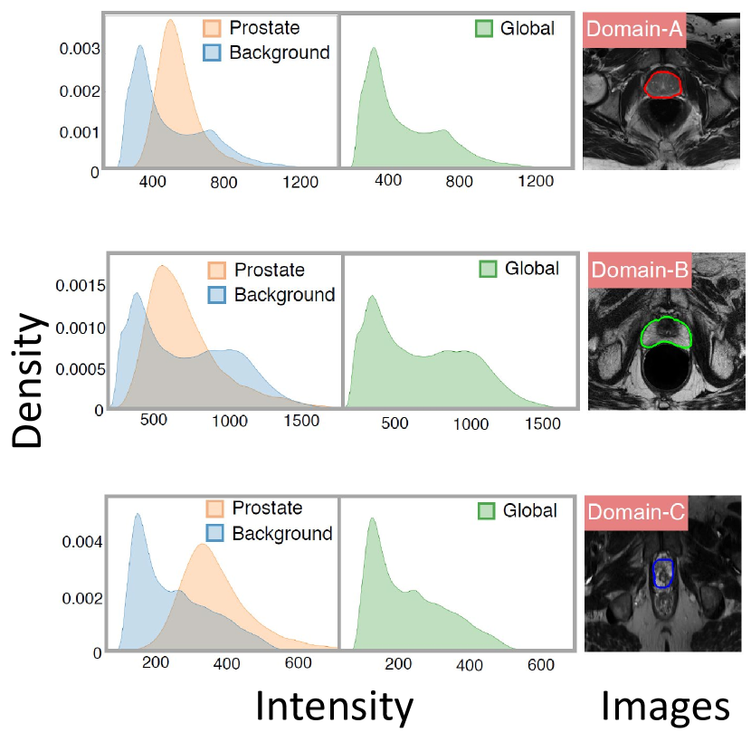
Normalization techniques are vital to accelerate and stabilize the network training procedure. In addition to batch normalization (BN) [13], alternative techniques have been used, such as group normalization [25], layer normalization [1], and instance normalization [24]. However, these normalization strategies are found to be suboptimal for medical image segmentation [19] because they only estimate the statistics of the images as a whole, which can be easily biased towards the intensity distribution of dominant categories (see Figure 1).

To address this problem, this paper focuses on enhancing BN with the intensity distribution of foreground pixels—the one that matters for image segmentation. We propose a new normalization strategy, named categorical normalization, named CateNorm, to normalize the activations according to categorical statistics. We introduce CateNorm to the U-Net architecture by enforcing the normalization layers to modulate foreground regions (e.g., pancreas, stomach) differently. Specifically, two parallel and complementary schemes are adopted for normalizing the activations—one is the conventional BN to capture the statistics of a batch of images; the other is the proposed CateNorm to integrate the statistics of specific regions with the guidance from the learned categories. As CateNorm conditions on the categorical masks (not available in the inference phase), we hereby introduce a simple yet effective two-stage training strategy: concretely, we first train exclusively using BN for generating the categorical masks and then feed them to CateNorm for updating the semantic-related modulating parameters.

Our extensive experiments on five datasets show that the integration of categorical statistics into normalization strategies can better capture the domain-invariant information from different domain data, thereby robustifying the learned medical representation. Compared with the existing normalization techniques [1, 13, 24, 25], CateNorm achieves more precise and robust segmentation results in various applications, including multi-organ segmentation from CT images and prostate segmentation from MRI images. CateNorm also consistently improves over the previous state of the arts for multi-domain data. This result suggests that CateNorm not only extracts more discriminative features but also compensates for the statistical bias in small distribution shifts and domain gaps.

Our contributions are three-fold: (1) a novel normalization to integrate categorical statistics with BN’s general statistics, surpassing existing normalization techniques; (2) a light CateNorm residual block for the U-Net encoder, yielding a prominent performance gain with negligible additional parameters; (3) CateNorm achieves better robustness in complex and variable data distributions.

2 Related Work

Normalization is one of the keys to the success of deep networks. As the most commonly used normalization technique, batch normalization (BN) [13] enables training with larger learning rates and greatly mitigates general gradient issues. Besides, alternative normalization strategies have also been designed for specific scenarios: layer normalization (LN) [1] for recurrent neural networks, instance normalization (IN) [24] for style transfer, group normalization (GN) [25] for small-batch training, etc. Beyond the natural image domain, these normalization strategies have also been successfully applied to medical applications. For example, Kao et al. [15] apply GN for brain tumor segmentation; Isensee et al. [14] apply IN in a self-adaptive framework for various segmentation tasks; Chen et al. [4] apply LN in Transformers for abdominal multi-organ segmentation. A detailed comparison among different normalization strategies for medical semantic segmentation and cross-modality synthesis has been summarized in Zhou et al. [28] and Hu et al. [11]. To offer stronger affine transformation, the latest strategies [7, 12] utilize external data to denormalize the features. As class information could be “washed away” with previous strategies, SPADE [20] directly uses class masks to guide the normalization. In addition, for domain adaptation and multi-domain learning, other methods propose to modify BN by modulating [18] or calculating domain-specific [3, 19] statistics. Unlike existing strategies, this paper proposes a novel categorical normalization strategy for incorporating different types of statistics.

3 Categorical Normalization (CateNorm)

Proof of concept: A simple experiment is designed to illustrate how categorical statistics can better mitigate distribution shifts across domains. We align the input image distributions based on the categorical statistics obtained from different datasets. Then we jointly train these heterogeneous datasets on the aligned input images. With class-wise distribution alignment, the model gains an improvement of 0.7% (91.4% vs. 90.7%). This suggests that aligning the data distribution based on class-wise statistics can better mitigate domain shifts between datasets and therefore achieve better results in the joint training setting. This interesting observation further motivates us to design normalization strategies to further leverage local statistics during the learning process.

We devise a two-stage training paradigm. In the first stage, the network is trained with BN to generate the class masks, which are later fed to the second stage to normalize the distribution based on each category. Figure 2 presents the overall pipeline of our approach. In the following, we will first introduce our CateNorm Residual Block (CNRB), following with the overall training and testing pipeline of CateNorm.

CateNorm Residual Block: In addition to BN in residual blocks [10], we introduce categorical normalization scheme while keeping all other components the same (see Figure 2(b)). Let $x$ with the spatial resolution of $H\times W$ denotes the input feature map, with a batch of $N$ samples and $C$ number of channels. For the $n$-th sample at the $c$-th channel, $x_{n,c,i,j}$ denotes the associated activation value at spatial location $(i,j)$. Then a BN branch and a CateNorm branch are used for fully leveraging the general and categorical statistics, respectively. BN [13] estimates the statistics of a batch of images and then applies affine transformation with learnable parameters $\gamma^{\textup{BN}}_{c}$ and $\beta^{\textup{BN}}_{c}$ at the $c$-th channel. Specifically, we first compute the mean and standard deviation $\mu_{c}$ and $\sigma_{c}$ as follows: $\mu_{c}=\frac{1}{NHW}\sum_{n,i,j}x_{n,c,i,j}$, $\sigma_{c}=\sqrt{\frac{1}{NHW}\sum_{n,i,j}\left(\left(x_{n,c,i,j}\right)^{2}-\left(\mu_{c}\right)^{2}\right)+\epsilon}$, where $\epsilon$ denotes a small constant for avoiding invalid denominators. And the associated activation map can be then computed as:

$$\centering\gamma^{\textup{BN}}_{c}\cdot\frac{x_{n,c}-\mu_{c}}{\sigma_{c}}+\beta^{\textup{BN}}_{c}.\@add@centering$$ (1)

Figure 2: Framework overview: (a) architecture & training stages of U-Net using BN and CateNorm; (b) design of CateNorm residual block; (c) design of CateNorm.

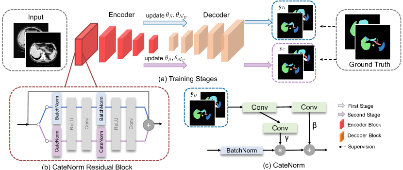
CateNorm serves as an addition normalization to integrate categorical statistics. The key difference, compared with BN, is that CateNorm provides a spatially-variant affine transformation which is learned from the corresponding class mask for modulating the activations. Therefore, the modulation parameters $\gamma^{\textup{CateNorm}}(\mathbf{m})$ and $\beta^{\textup{CateNorm}}(\mathbf{m})$ are no longer $C$-dimensional vectors as aforementioned, but tensors with spatial resolution $H\times W$. Here $\gamma^{\textup{CateNorm}}(\cdot)$ and $\beta^{\textup{CateNorm}}(\cdot)$ are learnable functions that act on the given class mask $\mathbf{m}$.

The activations of the CateNorm branch are computed as:

$$\centering\gamma^{\textup{CateNorm}}_{c,i,j}(\mathbf{m})\frac{x_{n,c,i,j}-\mu_{c}}{\sigma_{c}}+\beta^{\textup{CateNorm}}_{c,i,j}(\mathbf{m}).\@add@centering$$ (2)

Inspired by SPADE [20], we use a lightweight two-layer convolutional network to learn the modulation functions $\gamma^{\textup{CateNorm}}(\cdot)$ and $\beta^{\textup{CateNorm}}(\cdot)$, where the first layer is set to output features of $C/2$ number of channels.

Training CateNorm: We inject CateNorm into popular segmentation models, such as U-Net [21] and DeepLabV3+ [5]. The model can be denoted by $\mathcal{F}(\cdot;\theta)$ parameterized by $\theta=\{\theta_{s},\theta_{\mathcal{N}_{B}},\theta_{\mathcal{N}_{C}}\}$. $\theta_{\mathcal{N}_{B}}$ denote the learnable modulating parameters used in the BN branch and $\theta_{\mathcal{N}_{C}}$ is the learning modulation function that requires the corresponding class mask as an input; the subscripts $\mathcal{N}_{B}$ and $\mathcal{N}_{C}$ here denote BN and CateNorm. $\theta_{s}$ stands for all other network parameters.

In the first stage, we exclusive train the model through the BN branch, i.e., only $\theta_{s}$ and $\theta_{\mathcal{N}_{B}}$ are updated. The goal of the first stage is not only to leverage the global statistics for accelerating training but also to provide class information for learning CateNorm parameters in the second stage. Specifically, the class mask generated from the first stage $\hat{\mathbf{y}}_{B}$ can be written as:

$$\hat{\mathbf{y}}_{B} =\mathcal{F}(\theta_{S},\theta_{\mathcal{N}_{B}};\mathbf{x}).$$ (3)

In the second training stage, we train exclusively on the CateNorm branch for exploiting the local statistics, i.e., only update network parameters $\theta_{s}$ and the learnable function $\theta_{\mathcal{N}_{C}}(\cdot)$. Given the class mask $\hat{\mathbf{y}}_{B}$, the normalization parameters $\theta_{\mathcal{N}_{C}}(\hat{\mathbf{y}}_{B})$ can be then computed via Equation (2), and the predicted mask in the second stage $\hat{\mathbf{y}}_{C}$ can be written as:

$$\hat{\mathbf{y}}_{C}=\mathcal{F}(\theta_{S},\theta_{\mathcal{N}_{C}}(\hat{\mathbf{y}}_{B});\mathbf{x}),$$ (4)

where $\hat{\mathbf{y}}_{C}$ denotes the softmax probability map from the CateNorm branch. With auxiliary class information integrated, this training step aims at enhancing discriminative features, which leads to more accurate and robust segmentation

Overall training objective: Given a pair of probability prediction $\hat{\mathbf{y}}$ and the associated ground truth $\mathbf{y}\in\mathbb{L}^{D}$, the Dice loss and the cross entropy loss are: $\mathcal{L}_{Dice}(\mathbf{y},\hat{\mathbf{y}})=\frac{1}{|\mathbb{L}|}\sum_{l}[1-\frac{2\sum_{i,j,l}y_{i,j,l}\cdot\hat{y}_{i,j,l}}{\sum_{i,j,l}(y_{i,j,l}^{2}+\hat{y}_{i,j,l}^{2})}]$, $\mathcal{L}_{CE}(\mathbf{y},\hat{\mathbf{y}})=-\frac{1}{D\cdot|\mathbb{L}|}\sum_{i,j,l}y_{i,j,l}\cdot\log(\hat{y}_{i,j,l})$, where $\hat{y}_{i,j,l}$ is the output probability of the $l$-th class ($l\in\mathbb{L}$) of at spatial location $i,j$. In our loss function, we use a weighted sum of these two losses, which can be written as: $\mathcal{L}(\mathbf{y},\hat{\mathbf{y}})=\lambda\mathcal{L}_{Dice}(\mathbf{y},\hat{\mathbf{y}})+(1-\lambda)\mathcal{L}_{CE}(\mathbf{y},\hat{\mathbf{y}})$, where $\lambda$ is the balance parameter. Therefore, our overall training objective over these two stages is:

$$\mathcal{L}_{total}=\alpha\mathcal{L}(\mathbf{y},\hat{\mathbf{y}}_{B})+(1-\alpha)\mathcal{L}(\mathbf{y},\hat{\mathbf{y}}_{C}),$$ (5)

where $\alpha$ is set as 1 in the first stage and 0 in the second stage, for updating $\{\theta_{s},\theta_{\mathcal{N}_{B}}\}$ and $\{\theta_{s},\theta_{\mathcal{N}_{C}}\}$ alternately. In the testing phase, the final prediction is obtained by forwarding twice with Equations (3) & (4) sequentially. The whole training procedure is summarized in Appendix Algorithm 1.

4 Experiments

4.1 Dataset and Benchmark

Prostate segmentation datasets: Following Liu et al. [19], we use prostate T2-weighted MRI collected from three different domains. (1) 30 samples from Radboud University Nijmegen Medical Centre; (2) 30 samples from Boston Medical Center. Both (1) and (2) are available from NCI-ISBI 2013 challenge (ISBI 13) dataset [2], therefore are denoted as “ISBN-R” and “ISBN-B”. (3) 19 samples from Initiative for Collaborative Computer Vision Benchmarking (I2CVB) dataset [17], denoted as “I2CVB”. Details of their acquisition protocols are included in Appendix §0.C.

Abdominal multi-organ segmentation datasets: We use abdominal CT images of two different domains. (1) 30 training cases from the Beyond the Cranial Vault (BTCV) dataset [16]; (2) 41 cases from the Cancer Image Archive (TCIA) Pancreas-CT dataset [6, 22, 23], where the multi-class annotation can be acquired from Gibson et al. [9]. For single-domain experimental settings, 8 organs (spleen, left kidney, right kidney, gallbladder, pancreas, liver, stomach, and aorta) are evaluated following the settings in Fu et al. [8] and Chen et al. [4]. For multi-domain experiments, right kidney and aorta are excluded and we evaluate the remaining 6 organs which are labeled in both datasets.

Table 1: CateNorm vs. three other normalization strategies under the single-domain setting. The performance is measured by Dice score (%). CN denotes our categorical normalization. We report the average performance on five-fold cross-validation, along with the statistic analysis (*$p<$0.5, **$p<$0.1, ***$p<$0.05) between the best and second best methods.

Method	Norm	BTCV	ISBN-R	ISBN-B	I2CVB
Baseline	BN	75.56	88.69	85.20	87.21
Baseline	BN	77.83	89.13	85.99	88.22
Baseline	BN	78.98	90.08	87.22	88.99
Baseline	IN	78.96	89.05	88.37	88.98
Baseline	GN	78.50	89.15	88.61	89.16
Ours (block 1)	CN	79.33	91.36	88.55	89.31
Ours (block 1-4)	CN	80.37**	91.41**	87.57	89.79**

Table 2: CateNorm vs. three other methods under the multi-domain setting. CN denotes our categorical normalization. We report the average performance on five-fold cross-validation, along with the statistic analysis (*$p<$0.5, **$p<$0.1, ***$p<$0.05) between ours (bolded) and the best previous method (DSBN [3]).

Method	Norm	BTCV	TCIA	ISBN-R	ISBN-B	I2CVB
Baseline	BN	82.64	87.33	91.50	90.46	90.34
DSBN	BN	82.67	87.83	91.98	90.22	90.10
MS-Net	BN	82.17	87.85	91.93	90.30	89.89
Ours (block1)	CN	83.28	88.22	92.12	90.76	90.33
Ours (block1-4)	CN	83.45*	88.38**	92.47***	91.17***	90.79*

4.2 Robust Performance on Single- & Multi-Domain Data

We compare the proposed CateNorm strategy with various normalization methods, including BN [13], IN [24], and GN [25]. In addition, for multi-domain settings, we also compare with state-of-the-art multi-domain learning approaches, including DSBN [3], MS-Net [19]. To ensure a fair comparison, we implement UNet with residual blocks in the encoder [19, 27] for all baseline methods.

Single-domain results: As shown in Table 1, even with strong data augmentation, our CateNorm still yield a solid performance gain on all four datasets. For instance, on the prostate dataset “ISBN-R” and the multi-organ segmentation dataset, CateNorm outperforms BN by a large margin of $1.33\%$ and $1.39\%$ in average Dice. While different normalization methods (e.g., GN, IN) may behave similarly, our CateNorm consistently achieves better results compared with all other methods. We also compare two different configurations of CateNorm: 1) CateNorm (block 1) only replaces the first encoder block with CNRB; 2) CateNorm (block 1-4) replaces all of the first four encoder blocks with CNRBs. For prostate segmentation, we find that both variants show a solid improvement while CateNorm (block 1) with only few additional parameters performs similarly as CateNorm (block 1-4) (i.e., $89.74\%$ vs. $89.59\%$). On the contrary, for multi-organ segmentation, block 1 demonstrates inferior results than block 1-4 (i.e., $79.33\%$ vs. $80.37\%$). This suggests that CNRB can bring additional benefits for complex tasks such as multi-organ segmentation. For the relatively simpler binary segmentation task, block 1 might be enough to learn a good model, therefore using more CNRBs does not lead to further performance gain. A detailed study regarding where to add CNRBs has been illustrated in §4.3.

Multi-domain segmentation results: We evaluate our method using the same multi-domain setting as in Liu et al. [19]. To demonstrate the effectiveness of CateNorm, we compare the performance with the baseline and state-of-the-art multi-domain learning methods (i.e., DSBN, MS-Net) on three prostate segmentation datasets and two multi-organ segmentation datasets. As shown in Table 2, under strong data augmentation (e.g., rotation, flipping), DSBN and MS-Net do not yield improvements anymore, while our method still secures a reasonable improvement compared to the baseline. For instance, block 1-4 outperforms the baseline by $0.81\%$ and $1.05\%$ in average Dice on the BTCV and TCIA dataset, respectively. This indicates that, unlike previous methods which customize the normalization layers for different domains [3, 19], our CateNorm can better extract domain-invariant information in the face of a more complex and variable data distribution. Meanwhile, it is also worth mentioning that our approach is complementary to previously domain-specific normalization methods.

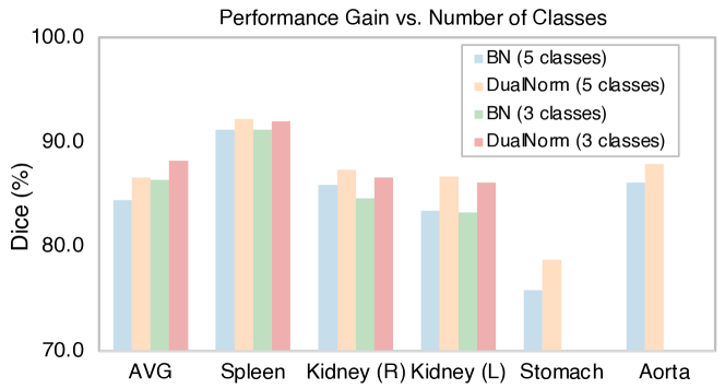
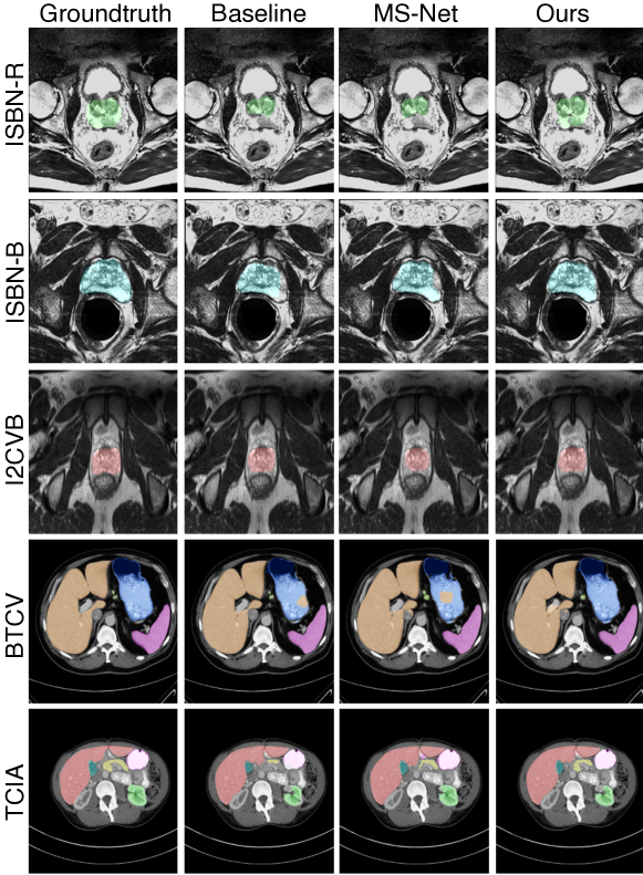
Unlike the single-domain setting, block 1-4 outperforms block 1 for both prostate segmentation and multi-organ segmentation. We conjecture that this is due to that given a more complex data distribution, more CNRBs can bring additional benefits by imposing semantic guidance on the encoder more densely. More importantly, our CateNorm is flexible to many popular segmentation architectures such as DeepLabV3+ (see Appendix Table 6). Moreover, CateNorm shows great robustness in partially annotated scenarios—detailed studies are provided in Appendix Figure 3. Qualitative results are in Appendix Figure 4.

4.3 Discussion and Ablation Study

Table 3: Parameter sharing for the two-stage normalization (Dice Score in %)

Method	Sharing	#Params	Dice
U-Net	–	1.0$\times$	90.08
W-Net	✗	2.073$\times$	90.36
Ours(blk1)	✓	1.001$\times$	91.36
Ours(blk1-4)	✓	1.073$\times$	91.41

(a) Sharing vs. no-sharing

	Forward	Prostate	Abdominal
Baseline	BN	90.76	84.98
Ours	BN	91.00	85.39
	CN	91.48	85.92

(b) Mutual benefits of BN and CateNorm.

Parameter sharing for the two-stage normalization: To prove the necessity of network sharing except the normalization layers, we also implement our method by using different network parameters $\theta_{s}$ in the two training stages, similar to W-Net [26]. In this implementation, CateNorm and BN are deployed in two independent sub-networks, which are simply concatenated for training and testing. As shown in Table 3a, our method performs much better than W-Net with only about 50% of the parameters. Besides, even only comparing the results in the first stage where only BN is used during inference, as shown in Table 3b, our approach still outperforms the baseline by $0.24\%$ and $0.41\%$ in average Dice. Then in the second stage where CateNorm is used for inference, the performance can be further improved by $0.48\%$ and $0.53\%$. This indicates that by sharing the rest of the network parameters, the two normalization schemes can mutually benefit each other by leveraging both general and categorical statistics.

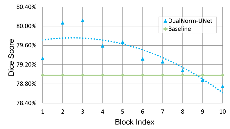
Adding CateNorm to the earlier encoder: As shown in §4.2, adding more CateNorm in the U-Net encoder can benefit both prostate and multi-organ segmentation, especially under the multi-domain setting. This observation motivates us to further investigate where to add CateNorm, as this can help us design better configurations of CateNorm which achieve higher performance without incurring much computation cost. In our experiments, U-Net consists of 5 encoder blocks and 5 decoder blocks. By varying the position to add the CateNorm from blocks 1 to 10, we compare the average Dice score on the BTCV dataset. As shown in Appendix Figure 5, CateNorm blocks are preferred to be set in early blocks (encoder).

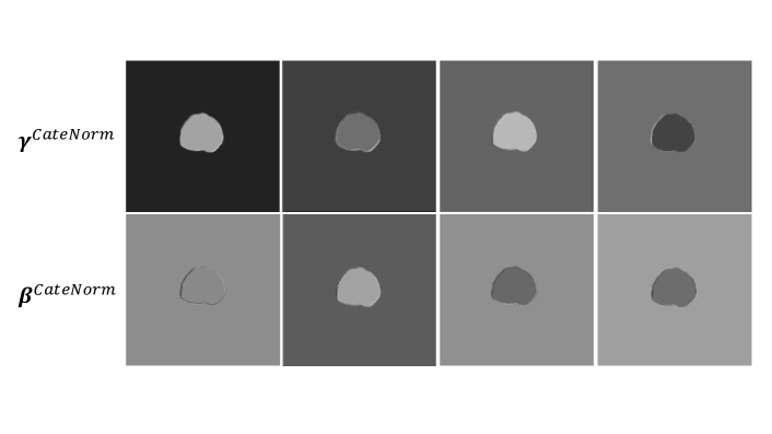
Visualizing activations in CateNorm: Appendix Figure 6 visualizes the learned $\gamma^{\textup{CateNorm}}$ and $\beta^{\textup{CateNorm}}$ on different channels of the intermediate CateNorm layers during the second forward. With prior class information as guidance, CateNorm can modulate spatially-adaptive parameters. Such spatial-wise modulation can be complementary to the channel-wise modulation accomplished by BN, and derives more discriminative features that benefit segmentation.

5 Conclusion

We have presented a new normalization strategy, named CateNorm, which complementarily enhance the categorical statistics in BN for robust medical image segmentation. Our CateNorm can be used as an add-on to existing segmentation architectures, such as U-Net and DeepLabV3+. Compared with existing normalization strategies, CateNorm consistently achieves superior results, even with complex and variable data distributions. We believe that the proposed normalization strategy could also improve natural image segmentation and plan to explore it in the future work.

Acknowledgments: This work was supported by the Lustgarten Foundation for Pancreatic Cancer Research. We also thank Quande Liu for the discussion.

Appendix 0.A Details of Aligning Input Distribution Algorithm

Assume that we have $N$ source domains $S_{1},S_{2},S_{3},...,S_{N}$, with $M_{1},M_{2},M_{3},...,M_{N}$ examples respectively, where the $i$-th domain source domain $S_{i}$ consists of an image set $\{\mathbf{x}_{i,j}\in\mathbb{R}^{D_{i,j}}\}_{j=1,...,M_{i}}$ as well as their associated annotations. Our goal is to align the image distributions of these source domains with the target domain $T$ based on the class-wise (region-wise) statistics. The algorithm can be illustrated as the following steps:

Step 1: Calculate class-wise statistics of each case

Firstly, we calculate the mean and standard deviation of each case in both the source domain and the target domain.

$$\centering\mu_{i,j}^{c}\@add@centering =\frac{\sum_{k=1}^{|D^{c}_{i,j}|}\mathbf{x}^{c}_{i,j,k}}{|D^{c}_{i,j}|},$$ (6)

$$\sigma_{i,j}^{c} =\sqrt{\frac{1}{|D^{c}_{i,j}|}\sum_{k=1}^{|D^{c}_{i,j}|}(\mathbf{x}^{c}_{i,j,k}-\mu_{i,j}^{c})^{2}},$$ (7)

where $\mathbf{x}_{i,j}^{c}$ denotes the pixels which belong to the $c$-th class (region) in image $\mathbf{x}_{i,j}$, with the number of pixels denoted as $|D^{c}_{i,j}|$. As a special case, $i=T$ indicates the target domain.

Step 2: Estimate aligned (new) class-wise statistics

Next, we calculate the mean of the statistics over all examples obtained in each domain as follows:

$$\centering\bar{\mu}_{i}^{c}\@add@centering =\frac{\sum_{j=1}^{M_{i}}\mu_{i,j}^{c}}{M_{i}},$$ (8)

$$\bar{\sigma}_{i}^{c} =\frac{\sum_{j=1}^{M_{i}}\sigma_{i,j}^{c}}{M_{i}}.$$ (9)

Based on the $\bar{\mu}_{i}^{c}$, we now estimate the new class-wise mean $\tilde{\mu}_{i,j}$ for each case of the source domain $S_{i}$ as follows:

$$\begin{split}\tilde{\mu}_{i,j}^{c}&=\frac{\mu_{i,j}^{c}-\bar{\mu}_{i}^{c}}{\sqrt{\frac{\sum_{j=1}^{M_{i}}(\mu_{i,j}^{c}-\bar{\mu}_{i}^{c})^{2}}{M_{i}}}}\cdot\sqrt{\frac{\sum_{j=1}^{M_{T}}(\mu_{T,j}^{c}-\bar{\mu}_{T}^{c})^{2}}{M_{T}}}+\bar{\mu}_{T}^{c},\\ \end{split}$$ (10)

where $M_{T}$ denotes the number of cases in the target domain $T$. Similarly, the new standard deviation $\tilde{\sigma}_{i,j}$ can be computed by:

$$\begin{split}\tilde{\sigma}_{i,j}^{c}&=\frac{\sigma_{i,j}^{c}-\bar{\sigma}_{i}^{c}}{\sqrt{\frac{\sum_{j=1}^{M_{i}}(\sigma_{i,j}^{c}-\bar{\sigma}_{i}^{c})^{2}}{M_{i}}}}\cdot\sqrt{\frac{\sum_{j=1}^{M_{T}}(\sigma_{T,j}^{c}-\bar{\sigma}_{T}^{c})^{2}}{M_{T}}}+\bar{\sigma}_{T}^{c}.\\ \end{split}$$ (11)

Step 3: Align each case with the estimated statistics

Based on the computed new mean and standard deviation $\tilde{\mu}_{i,j}$, $\tilde{\sigma}_{i,j}$, the aligned image $\tilde{\mathbf{x}}_{i,j}$ can be computed as:

$$\centering\tilde{\mathbf{x}}_{i,j}^{c}\@add@centering =\frac{\mathbf{x}_{i,j}^{c}-\mu_{i,j}^{c}}{\sigma_{i,j}^{c}}\cdot\tilde{\sigma}_{i,j}^{c}+\tilde{\mu}_{i,j}^{c}.$$ (12)

Appendix 0.B Implementation Details

Table 4: Data Preprocessing.

Step	Prostate	Abdominal
1	Center-cropping	Window range Clipping [-125, 275]
2	Out-of-mask slice cropping	Out-of-mask slice cropping
3	Resizing	Resizing
4	Z-score Normalization	Z-score Normalization

Table 5: Experimental Setting.

config	value
training iterations	9000
optimizer	Adam
initial learning rate	1e-3
optimizer momentum	$\beta_{1},\beta_{2}{=}0.9,0.999$
batch size	4 (single) 6 (multi)
learning rate schedule	plateau scheduler
Dice/CE balance factor $\lambda$	0.5 (abdominal) 1.0 (prostate)
augmentation	horizontal flipping (prostate only) + random rotation
validation strategy	5-fold
evaluation metric	Dice Score (%) and ASD (mm)

Appendix 0.C Details of the Prostate Datasets

Table 6: Details of the 3 prostate segmentation datasets.

Dataset	#Cases	Field strength (T)	Resolution (in/through plane)	Manufacturer
ISBN-R	30	3	0.6-0.625/3.6-4	Siemens
ISBN-B	30	1.5	0.4/3	Philips
I2CVB	19	3	0.67-0.79/1.25	Siemens

Appendix 0.D Training procedure of CateNorm

Algorithm 1 Training procedure of CateNorm

0:  Images and labels $\mathbf{x}$, $\mathbf{y}$;        Network parameters $\theta=\{\theta_{S},\theta_{\mathcal{N}_{B}},\theta_{\mathcal{N}_{C}}\}$;        Training iterations $\tau$;

0:  Optimized parameters $\theta_{S}$, $\theta_{\mathcal{N}_{B}}$, $\theta_{\mathcal{N}_{C}}$;

1:  t $\leftarrow$ 0;

2:  Initialize $\theta_{S}$, $\theta_{\mathcal{N}_{B}}$ with the pretrained model and randomly initialize $\theta_{\mathcal{N}_{C}}$;

3:  while $t<\tau$ do

4:     Compute the class mask $\hat{\mathbf{y}}_{B}$;

5:     $\alpha\leftarrow 1$;

6:     Update ${\theta_{s},\theta_{\mathcal{N}_{B}}}\leftarrow\mathop{\mathrm{min}_{\theta_{s},\theta_{\mathcal{N}_{B}}}}{\mathcal{L}_{total}}$;

7:     Detach $\hat{\mathbf{y}}_{B}$ from gradient calculation;

8:     Compute the class mask $\hat{\mathbf{y}}_{C}$;

9:     $\alpha\leftarrow 0$;

10:     Update ${\theta_{s},\theta_{\mathcal{N}_{C}}(\cdot)}\leftarrow\mathop{\mathrm{min}_{\theta_{s},\theta_{\mathcal{N}_{C}}}}{\mathcal{L}_{total}}$;

11:     $t\leftarrow t+1$;

12:  end while

Appendix 0.E Average Surface Distance (ASD) Comparison

The detailed average surface distance results of both prostate segmentation and abdominal segmentation tasks can be found in Tables 7 and 8. the proposed CateNorm achieves the lowest average ASD on both tasks, even under the more challenging multi-domain setting.

Table 7: ASD comparison on the abdominal datasets under the multi-domain setting (in mm). Compared with the baseline and other competitive methods, the proposed CateNorm achieves the lowest average ASD.

Method	Forward	BTCV	TCIA	AVG	Spleen	Kid.(L)	Gall.	Liver	Stom.	Panc.
Baseline	BN	1.28	1.17	1.22	0.59	0.59	2.36	0.77	1.93	1.10
DSBN [3]	BN	1.86	0.90	1.38	0.51	0.79	3.07	0.76	1.96	1.19
MS-Net [19]	BN	1.61	1.02	1.31	0.52	0.75	2.91	0.91	1.58	1.21
Ours (block1)	CN	1.22	1.10	1.16	0.54	0.58	2.22	0.74	1.76	1.10
Ours (block1-4)	CN	1.64	0.97	1.30	0.51	0.55	3.25	0.75	1.75	1.01

Table 8: ASD comparison on prostate segmentation datasets under the multi-domain setting (in mm). Compared with the baseline and other competitive methods, the proposed CateNorm achieves the lowest average ASD.

Method	Norm	ISBN-R	ISBN-B	I2CVB	AVG
Baseline	BN	0.64	0.71	1.22	0.86
DSBN [3]	BN	0.56	0.69	1.17	0.81
MS-Net [19]	BN	0.58	0.70	1.32	0.87
Ours (block1)	CN	0.63	0.66	1.27	0.85
Ours (block1-4)	CN	0.54	0.64	1.13	0.77

Figure 3: Performance gain under partial annotation. We compare our method to the baseline with fewer annotated classes (i.e., 3/5). We can see that by partitioning the images into different number of regions, CateNorm consistently achieves better results than BN for all tested organs. This suggests that our algorithm is not sensitive to the number of regions.

Figure 4: Qualitative results comparison. We compare our baseline and the other SOTA method under the multi-domain setting on prostate segmentation and abdominal multi-organ segmentation. Results in the first three rows clearly show that our method outperforms others as their results are cracked and incomplete with these unapparent prostate boundaries. And the results in the last two rows show our methods could better suppress inconsistent class information inside a close segmented area (e.g., reducing false positives inside the stomach) and predict hard organs like the pancreas more accurately by incorporating general and categorical statistics.

Table 4: Comparison on the multi-organ segmentation dataset (BTCV) with single-domain setting (Dice Score in %).

Method	Pretrained	Aug	Norm	AVG	Spleen	Kidney (R)	Kidney (L)	Gallbladder	Pancreas	Liver	Stomach	Aorta
Baseline	✗	✗	BN	75.56	92.00	81.92	84.45	50.76	48.89	95.07	68.25	83.16
Baseline	✗	✓	BN	77.83	91.86	84.36	86.99	53.92	51.18	95.11	75.24	83.97
Baseline	✓	✓	BN	78.98	93.43	84.68	87.98	54.54	55.14	95.35	76.19	84.49
Baseline	✓	✓	IN	78.96	91.93	83.70	87.83	54.29	55.08	95.23	78.72	84.93
Baseline	✓	✓	GN	78.50	89.84	85.64	86.26	55.14	55.70	94.71	75.98	84.71
Ours(blk1)	✓	✓	CN	79.33	93.07	85.66	88.26	52.79	54.34	95.64	77.38	87.49
Ours(blk-4)	✓	✓	CN	80.37	94.63	86.29	88.64	55.51	55.91	95.64	79.80	86.52

Table 5: Organ-wise results on the multi-organ segmentation datasets under the multi-domain setting (Dice Score in %).

Method	Norm	BTCV	TCIA	AVG	Spleen	Kidney (L)	Gallbladder	Liver	Stomach	Pancreas
Baseline	BN	82.64	87.33	84.98	95.22	93.54	69.63	96.01	85.52	69.97
DSBN	BN	82.67	87.83	85.25	95.42	93.49	69.98	96.16	86.11	70.34
MS-Net	BN	82.17	87.85	85.01	95.36	93.10	68.38	95.75	86.77	70.69
Ours (block1)	CateNorm	83.28	88.22	85.75	95.45	93.63	70.79	96.13	87.18	71.32
Ours (block1-4)	CateNorm	83.45	88.38	85.92	95.55	93.48	71.53	96.13	87.20	71.60

Table 6: CateNorm is compatible to other segmentation models. This table compares performance on multi-domain multi-organ and prostate segmentation with DeepLabv3+ [5] architecture. Our CateNorm consistently outperforms BN.

Backbone	Norm	AVG	BTCV	TCIA
DeepLabV3+	BN	84.58	81.33	87.83
DeepLabV3+	CN	85.42	82.13	88.72
		AVG	ISBN-R	ISBN-B	I2CVB
DeepLabV3+	BN	88.54	90.73	89.35	85.55
DeepLabV3+	CN	89.21	91.26	89.78	86.59

Table 7: CateNorm is not sensitive to the warmup length.. This table reports average accuracy (%) of our CateNorm under deteriorated pretrained models with fewer pretraining iterations. We reduce the warmup iterations to 450, 1440, and 9000 for multi-domain prostate segmentation experiments, to investigate how our CateNorm performs when warmuped with less iterations.

Warmup Iters	450	1440	9000
Warmup Acc.	73.91%	82.32%	90.10%
Ours Acc.	91.16%	91.17%	91.48%

Figure 5: Set CateNorm block(s) early. This table compares performance with single CateNorm block set in different positions. Adding the CateNorm to the encoder (block index 1-5) always yields better performance than adding to the decoder (block index 6-10). In general, the performance decreases as the block index increases. We believe that it is because the earlier layers in the encoder extract lower-level features that are less discriminative than the decoder features.

Figure 6: CateNorm does normalize with semantic information. This figure visualizes the learned $\gamma^{\textup{CateNorm}}$ (1st row) and $\beta^{\textup{CateNorm}}$ (2nd row) of a CateNorm layer in a CateNorm block on different channels of the intermediate CateNorm layer during the second forward. With prior class information as guidance, CateNorm can modulate spatially-adaptive parameters. Such spatial-wise modulation can be complementary to the channel-wise modulation accomplished by BN, and derives more discriminative features that benefit segmentation.

References

- [1] Ba, J.L., Kiros, J.R., Hinton, G.E.: Layer normalization (2016)
- [2] Bloch, N., Madabhushi, A., Huisman, H., Freymann, J., Kirby, J., Grauer, M., Enquobahrie, A., Jaffe, C., Clarke, L., Farahani, K.: Nci-isbi 2013 challenge: Automated segmentation of prostate structures. (2015), the Cancer Imaging Archive. http://doi.org/10.7937/K9/TCIA.2015.zF0vlOPv
- [3] Chang, W.G., You, T., Seo, S., Kwak, S., Han, B.: Domain-specific batch normalization for unsupervised domain adaptation. In: Proceedings of the IEEE/CVF Conference on Computer Vision and Pattern Recognition. pp. 7354–7362 (2019)
- [4] Chen, J., Lu, Y., Yu, Q., Luo, X., Adeli, E., Wang, Y., Lu, L., Yuille, A.L., Zhou, Y.: Transunet: Transformers make strong encoders for medical image segmentation (2021)
- [5] Chen, L.C., Zhu, Y., Papandreou, G., Schroff, F., Adam, H.: Encoder-decoder with atrous separable convolution for semantic image segmentation. In: Proceedings of the European conference on computer vision (ECCV). pp. 801–818 (2018)
- [6] Clark, K., Vendt, B., Smith, K., Freymann, J., Kirby, J., Koppel, P., Moore, S., Phillips, S., Maffitt, D., Pringle, M., et al.: The cancer imaging archive (tcia): maintaining and operating a public information repository. Journal of digital imaging 26(6), 1045–1057 (2013)
- [7] Dumoulin, V., Shlens, J., Kudlur, M.: A learned representation for artistic style. In: 5th International Conference on Learning Representations, ICLR 2017, Toulon, France, April 24-26, 2017, Conference Track Proceedings. OpenReview.net (2017), https://openreview.net/forum?id=BJO-BuT1g
- [8] Fu, S., Lu, Y., Wang, Y., Zhou, Y., Shen, W., Fishman, E., Yuille, A.: Domain adaptive relational reasoning for 3d multi-organ segmentation. In: International Conference on Medical Image Computing and Computer-Assisted Intervention. pp. 656–666. Springer (2020)
- [9] Gibson, E., Giganti, F., Hu, Y., Bonmati, E., Bandula, S., Gurusamy, K., Davidson, B., Pereira, S.P., Clarkson, M.J., Barratt, D.C.: Multi-organ Abdominal CT Reference Standard Segmentations (Feb 2018). https://doi.org/10.5281/zenodo.1169361, https://doi.org/10.5281/zenodo.1169361
- [10] He, K., Zhang, X., Ren, S., Sun, J.: Deep residual learning for image recognition. In: Proceedings of the IEEE conference on computer vision and pattern recognition. pp. 770–778 (2016)
- [11] Hu, S., Yuan, J., Wang, S.: Cross-modality synthesis from mri to pet using adversarial u-net with different normalization. In: 2019 International Conference on Medical Imaging Physics and Engineering (ICMIPE). pp. 1–5. IEEE (2019)
- [12] Huang, X., Belongie, S.: Arbitrary style transfer in real-time with adaptive instance normalization. In: Proceedings of the IEEE International Conference on Computer Vision. pp. 1501–1510 (2017)
- [13] Ioffe, S., Szegedy, C.: Batch normalization: Accelerating deep network training by reducing internal covariate shift. In: International conference on machine learning. pp. 448–456. PMLR (2015)
- [14] Isensee, F., Kickingereder, P., Wick, W., Bendszus, M., Maier-Hein, K.H.: No new-net. In: International MICCAI Brainlesion Workshop. pp. 234–244. Springer (2018)
- [15] Kao, P.Y., Ngo, T., Zhang, A., Chen, J.W., Manjunath, B.: Brain tumor segmentation and tractographic feature extraction from structural mr images for overall survival prediction. In: International MICCAI Brainlesion Workshop. pp. 128–141. Springer (2018)
- [16] Landman, B., Xu, Z., Igelsias, J., Styner, M., Langerak, T., Klein, A.: 2015 miccai multi-atlas labeling beyond the cranial vault workshop and challenge (2015), doi:10.7303/syn3193805
- [17] Lemaître, G., Martí, R., Freixenet, J., Vilanova, J.C., Walker, P.M., Meriaudeau, F.: Computer-aided detection and diagnosis for prostate cancer based on mono and multi-parametric mri: a review. Computers in biology and medicine 60, 8–31 (2015)
- [18] Li, Y., Wang, N., Shi, J., Liu, J., Hou, X.: Revisiting batch normalization for practical domain adaptation (2016)
- [19] Liu, Q., Dou, Q., Yu, L., Heng, P.A.: Ms-net: Multi-site network for improving prostate segmentation with heterogeneous mri data. IEEE Transactions on Medical Imaging (2020)
- [20] Park, T., Liu, M.Y., Wang, T.C., Zhu, J.Y.: Semantic image synthesis with spatially-adaptive normalization. In: Proceedings of the IEEE/CVF Conference on Computer Vision and Pattern Recognition. pp. 2337–2346 (2019)
- [21] Ronneberger, O., Fischer, P., Brox, T.: U-net: Convolutional networks for biomedical image segmentation. In: International Conference on Medical image computing and computer-assisted intervention. pp. 234–241. Springer (2015)
- [22] Roth, H., Farag, A., Turkbey, E.B., Lu, L., Liu, J., Summers, R.M.: Data from pancreas-ct (2016). https://doi.org/10.7937/K9/TCIA.2016.TNB1KQBU, the Cancer Imaging Archive. https://doi.org/10.7937/K9/TCIA.2016.tNB1kqBU
- [23] Roth, H.R., Lu, L., Farag, A., Shin, H.C., Liu, J., Turkbey, E.B., Summers, R.M.: Deeporgan: Multi-level deep convolutional networks for automated pancreas segmentation. In: International conference on medical image computing and computer-assisted intervention. pp. 556–564. Springer (2015)
- [24] Ulyanov, D., Vedaldi, A., Lempitsky, V.: Instance normalization: The missing ingredient for fast stylization (2017)
- [25] Wu, Y., He, K.: Group normalization. In: Proceedings of the European conference on computer vision (ECCV). pp. 3–19 (2018)
- [26] Xia, X., Kulis, B.: W-net: A deep model for fully unsupervised image segmentation (2017)
- [27] Yu, L., Yang, X., Chen, H., Qin, J., Heng, P.A.: Volumetric convnets with mixed residual connections for automated prostate segmentation from 3d mr images. In: Thirty-first AAAI conference on artificial intelligence (2017)
- [28] Zhou, X.Y., Yang, G.Z.: Normalization in training u-net for 2-d biomedical semantic segmentation. IEEE Robotics and Automation Letters 4(2), 1792–1799 (2019)