Using Context for Creating Rich Explanations for Query Answers
Augmenting Provenance with Contextual Information for Rich Explanations
Putting Things into Context: Rich Explanations for Query Answers using Join Graphs
Abstract.
In many data analysis applications, there is a need to explain why a surprising or interesting result was produced by a query. Previous approaches to explaining results have directly or indirectly used data provenance (input tuples contributing to the result(s) of interest), which is limited by the fact that relevant information for explaining an answer may not be fully contained in the provenance. We propose a new approach for explaining query results by augmenting provenance with information from other related tables in the database. We develop a suite of optimization techniques, and demonstrate experimentally using real datasets and through a user study that our approach produces meaningful results by efficiently navigating the large search space of possible explanations.
tabsize=2, basicstyle=, language=SQL, morekeywords=PROVENANCE,BASERELATION,INFLUENCE,COPY,ON,TRANSPROV,TRANSSQL,TRANSXML,CONTRIBUTION,COMPLETE,TRANSITIVE,NONTRANSITIVE,EXPLAIN,SQLTEXT,GRAPH,IS,ANNOT,THIS,XSLT,MAPPROV,cxpath,OF,TRANSACTION,SERIALIZABLE,COMMITTED,INSERT,INTO,WITH,SCN,UPDATED,GROUPING, extendedchars=false, keywordstyle=, mathescape=true, escapechar=@, sensitive=true
tabsize=2, basicstyle=, language=SQL, morekeywords=PROVENANCE,BASERELATION,INFLUENCE,COPY,ON,TRANSPROV,TRANSSQL,TRANSXML,CONTRIBUTION,COMPLETE,TRANSITIVE,NONTRANSITIVE,EXPLAIN,SQLTEXT,GRAPH,IS,ANNOT,THIS,XSLT,MAPPROV,cxpath,OF,TRANSACTION,SERIALIZABLE,COMMITTED,INSERT,INTO,WITH,SCN,UPDATED,GROUPING, extendedchars=false, keywordstyle=, deletekeywords=count,min,max,avg,sum, keywords=[2]count,min,max,avg,sum, keywordstyle=[2], stringstyle=, commentstyle=, mathescape=true, escapechar=@, sensitive=true
basicstyle=, language=prolog
tabsize=3, basicstyle=, language=c, morekeywords=if,else,foreach,case,return,in,or, extendedchars=true, mathescape=true, literate=:=1 ¡=1 !=1 append1 calP2, keywordstyle=, escapechar=&, numbers=left, numberstyle=, stepnumber=1, numbersep=5pt,
tabsize=3, basicstyle=, language=xml, extendedchars=true, mathescape=true, escapechar=£, tagstyle=, usekeywordsintag=true, morekeywords=alias,name,id, keywordstyle=
1. Introduction
Today’s world is dominated by data. Recent advances in complex analytics enable businesses, governments, and scientists to extract value from their data. However, results of such operations are often hard to interpret and debugging such applications is challenging, motivating the need to develop approaches that can automatically interpret and explain results to data analysts in a meaningful way. Data provenance (Green et al., 2007a; Cheney et al., 2009), which has been studied for several decades, is an immediate form of explanations that describes how an answer is derived from input data. However, provenance is often insufficient for unearthing interesting insights from the data that led to a surprising result, especially for aggregate query answers. In the last few years, several “explanation” methods have emerged in the data management literature (Barman et al., 2007; Wu and Madden, 2013; Roy and Suciu, 2014; Gebaly et al., 2014; ten Cate et al., 2015; Roy et al., 2015; Miao et al., 2019; Wang and Meliou, 2019) that return insightful answers in response to questions from a user. However, real world data often exhibits complex correlations and inter-relationships that connect the provenance of a query with data that has not been accessed by the query. Current approaches do not take these crucial inter-relationships into account. Thus, the explanations they produce may lack important contextual information that can aid the user in developing a deeper understanding of the results. We illustrate how to use context to explain a user’s question using data extracted from the official website of the NBA (NBA.com, 2020).
Example 0.
Consider a simplified NBA database with the following relations (the keys are underlined, the full schema has 11 relations). Some tuples from each relation are shown in Figure 1. Each team participating in a game can use multiple lineups consisting of five players. Home refers to the home team in a game.
-
•
Game(year, month, day, home, away, home_pts, away_pts, winner, season): participating teams and the winning team.
-
•
PlayerGameScoring(player, year, month, day, home, pts): the points each player scored in each game he played in.
-
•
LineupPerGameStats(lineupid, year, month, day, home,
mp): the minutes played by each lineup. -
•
LineupPlayer(lineupid, player): players for a lineup.
Suppose we are interested in exploring the winning records of the team GSW (Golden State Warriors) in every season. The following query returns this information:
Figure 1(e) shows the number of games team won for each season. made history in the NBA in the 2015-16 season to be the team that won the most games in a single season. Observe that team GSW improved its performance significantly from season 2012-13 () to season 2015-16 (). Such a drastic increase in a relatively short period of time naturally raises the question of what changed between these 2 seasons (denoted as the user question in Figure 1(f)). Note that only the Game table (shown in Figure 1(a)) was accessed by . This table provides the user with information about each game such as the name of the opponent team or whether was the home team or not. However, such information is not enough for understanding why won or lost more games than in the other seasons, since in each season a team would play the same number of games and home games, and roughly the same number of times against each opponent.
| year | mon | day | home | away | home_pts | away_pts | winner | season | |
| 2013 | 01 | 02 | MIA | DAL | 119 | 109 | MIA | 2012-13 | |
| 2012 | 12 | 05 | DET | GSW | 97 | 104 | GSW | 2012-13 | |
| 2015 | 10 | 27 | GSW | NOP | 111 | 95 | GSW | 2015-16 | |
| 2014 | 01 | 05 | GSW | WAS | 96 | 112 | GSW | 2013-14 | |
| 2016 | 01 | 22 | GSW | IND | 122 | 110 | GSW | 2015-16 |
| lineupid | player |
| 58420 | K. Thompson |
| 58420 | D. Green |
| 13507 | S. Battier |
| 13507 | L. James |
| 67949 | D. Green |
| player | year | mon | day | home | pts | |
| 2012 | 12 | 05 | DET | 22 | ||
| 2015 | 10 | 27 | GSW | 40 | ||
| 2016 | 01 | 22 | GSW | 39 | ||
| 2012 | 12 | 05 | DET | 27 | ||
| 2016 | 01 | 22 | DET | 18 | ||
| 2012 | 12 | 05 | DET | 2 |
| lineupid | year | mon | day | home | mp |
| 13507 | 2013 | 11 | 09 | MIA | 4.30 |
| 77727 | 2012 | 12 | 12 | MIA | 14.70 |
| 58420 | 2015 | 11 | 07 | SAC | 10.30 |
| 58482 | 2015 | 11 | 07 | SAC | 11.10 |
| 58420 | 2014 | 12 | 08 | MIN | 11.70 |
| team | season | win | |
| 2012-13 | 47 | ||
| 2013-14 | 51 | ||
| 2014-15 | 67 | ||
| 2015-16 | 73 | ||
| 2016-17 | 67 |
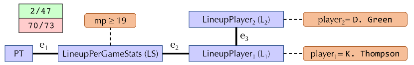
In this paper, we present an approach that answer questions like (Figure 1(f)). Our approach produces insightful explanations that are based on contextual information mined from tables that are related to the tables accessed by a user’s query. To give a flavor of the explanations produced by our approach, we present two of the top explanations for in Figures 2 and 2 (the formal definitions and scoring function are presented in the next section). Each explanation consists of three elements: (1) A join graph consisting of a node labeled PT representing the table(s) accessed by the user’s query (we refer to this as the provenance table, or PT for short), and nodes representing other tables that were joined with the provenance table to provide the context. Edges in a join graph represent joins between two tables. Each edge is labeled with the join condition that was used to connect the tables. (2) A pattern, which is a conjunction of predicates on attributes from the provenance or any table from the context. (3) The support of the pattern in terms of the number of tuples from the provenance of each of the two result tuples from the user question that are covered by the pattern (bold and underlined in the explanations shown below, formally defined in Section 2.5).
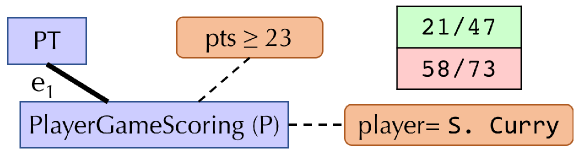
= (PT.year=P.year PT.month=P.month PT.day=P.day PT.home=P.home)
-
= (PT.year=LS.year PT.month=LS.month PT.day=LS.day PT.home=LS.home)
-
= (LS.lineupid = .lineupid) = (.lineupid = .lineupid)
Intuitively, the explanation from Figure 2 can be interpreted as:
Given this explanation, the user can infer that S. Curry was one of the key contributors for the improvement of GSW’s winning record since his points significantly improved in the season. Similarly, the explanation in Figure 2 can be interpreted as:
This implies that Green and Thompson’s increase of playing time together might have helped improve ’s record. We will discuss other example queries, user questions, and explanations returned by our approach using the NBA and the MIMIC hospital records dataset (Johnson et al., 2016) in Section 6.
Our Contributions. In this paper, we develop CaJaDE (Context-Aware Join-Augmented Deep Explanations), the first system that automatically augments provenance data with related contextual information from other tables to produce more informative summaries of the difference between the values of two tuples in the answer of an aggregate query, or, the high/low value of a single outlier tuple. We make the following contributions in this paper.
(1) Join-augmented provenance summaries as explanations. We propose the notion of join-augmented provenance and use summaries of augmented provenance as explanations. The join-augmented provenance is generated based on a join graph that encodes how the provenance should be joined with tables that provide context. We use patterns, i.e., conjunctions of equality and inequality predicates, to summarize the difference between the join-augmented provenance of two tuples from a query’s output selected by the user’s question. We adapt the notion of F-score to evaluate the quality of patterns . A high F-score is likely to combine two desired properties for the summary distinguishing and by giving preference to patterns with (i) high recall (the pattern covers many tuples in the provenance of ) and (ii) high precision (the pattern does not cover many tuples in the provenance of ). (Section 2)
(2) Mining patterns over augmented provenance. We present algorithms for mining patterns for a given join graph and discuss a number of optimizations. Even if we fix a single join graph to compute the augmented provenance, the large number of possible patterns poses challenges to efficiently mining patterns with high F-score values. Our optimizations include clustering and filtering attributes using machine learning methods, using a monotonicity property for the recall of patterns to prune refinements of patterns (patterns are refined by adding additional predicates), and finding useful patterns on categorical attributes before considering numeric attributes to reduce the search space. (Section 3).
(3) Mining join graphs giving useful patterns. We also address the challenge of mining patterns over different join graphs that are based on a schema graph which encodes which joins are permissible in a schema. We prune the search space by estimating the cost of pattern mining as well as detecting from the available join patterns if the join graph is unlikely to generate high quality patterns. (Section 4)
(4) Qualitative and quantitative evaluation. We quantitatively evaluated the explanations produced by our approach using a case study using two real world datasets: NBA and MIMIC. We further conducted a user study to evaluate how useful the explanations generated by our approach are and how they compare with explanations generated based on the original provenance alone (Section 6). We conducted performance experiments using the NBA and MIMIC database to evaluate scalability varying parameters of our algorithms, and demonstrate the effectiveness of our optimizations. (Section 5)
2. Join-Augmented Provenance
A database comprises a set of relations . We will use and both for the schema and the instance where it is clear from the context. For a relation , denotes the set of attributes in ; similarly, for a set of relations , denotes the set of attributes in relations in . Without loss of generality, we assume the attribute names are distinct and use for disambiguation if an attribute appears in multiple relations. In this work we focus on simple single-block SQL queries with a single aggregate function (select-from-where-group by), or, equivalently extended relational algebra queries with the same restriction.111Extensions are discussed in Section 8. Given a query , denotes the result of evaluating the query over a database . We use to denote the relations accessed by .
2.1. Provenance Table
A large body of work has studied provenance semantics for various classes of queries (e.g., (Green et al., 2007a; Cheney et al., 2009)). Here we resort to a simple why-provenance (Cheney et al., 2009) model sufficient for our purpose. We define the provenance of an output tuple of a query as a subset of the cross product () of all relations in . For instance, Perm (Glavic and Alonso, 2009) can produce this type of provenance for queries in relational algebra plus aggregation and nested subqueries. In our implementation we use the GProM system (Arab et al., 2018).
Definition 1 (Provenance Table).
Given a with , we define the provenance table for and to be a subset of . We assume the existence of a provenance model that determines which tuples from the cross product belong to . For a tuple , we define the provenance table to be the subset of the provenance that contributes to (decided by the provenance model).
Example 0.
In Example 1.1, contains all the tuples from Figure 1(a) which has as the winner, i.e., , and . For as shown in Table 1(e), includes all the tuples where GSW won in the season, i.e., , and contains and .
2.2. Schema Graph s and Join Graph s
,
Schema graphs. As mentioned in the introduction, we create explanations by summarizing provenance augmented with additional information produced by joining the provenance with related tables. We assume that a schema graph is given as input that models which joins are allowed. The vertices of schema graph correspond to the relations in the database. Each edge in this graph encodes a possible join between the connected relations, and is labeled with a set of possible join conditions between the two connected relations. We use Cond to denote the set of all predicates involving Boolean conjunctions () and equality (=) of two attributes or an attribute with a constant that can be used for joining relations in (i.e., only equi-joins are allowed, although all common attributes do not have to be used as in natural joins).
Definition 2 (Schema Graph).
Given a database schema , schema graph for is an undirected edge-labeled graph with nodes , edges , and a labeling function that associates a set of conditions with every edge from . We require that for each edge , each condition in only references attributes from relations adjacent to .
Note that is an input for our method. To create schema graphs, our system can extract join conditions from the foreign key constraints of a database and also allows the user to provide additional join conditions. Furthermore, could be determined using join discovery techniques such as (Fernandez et al., 2018; Zhu et al., 2019; Sarma et al., 2012). Figure 3 shows the simplified schema graph for the NBA dataset discussed in Example 1.1. Unused relations in examples above are omitted. In the schema graph, relations are represented by nodes and are connected through edges () with conditions as labels. For example, in Figure 3 implies that we are allowed to join PlayerGameScoring(P) with Game(G) in two different ways: (1) through an equi-join on year, month, day, and home (i.e., the home-team of a game), which form the key of a game and therefore gives players’ stats in all the games they played, and (2) with an additional condition on home = winner, which gives players’ stats in the games when the home team won. Note that there is an edge which suggests node LineupPlayer(L) can be-joined with itself on condition L.lineupid = L.lineupid (renaming of is needed in the actual join) to find players in the same lineup.
Join graphs. A join graph encodes one possible way of augmenting with related tables in the schema. It contains a distinguished node representing the relations in . The other nodes of are labeled with relations, edges in are labeled with join conditions allowed by the schema graph , and there can be multiple parallel edges between two nodes ( is a multi-graph).
Definition 3 (join graph).
Given a database , schema graph and query , a join graph for is a node- and edge-labeled undirected multigraph with nodes , edges , a node labeling function , and edge labeling function . For any join graph we require that it contains exactly one node labeled with and there are no edges with as both end-points. For every edge we require that there exists a corresponding edge such that all of the following conditions hold:
-
•
(modulo renaming relations using their aliases for disambiguation as discussed below)
-
•
If , then , else,
-
•
If , then , else,
The first condition above says that the join condition between two relations in the join graph should be one of the allowed conditions in the schema graph . The second and third conditions say that edges adjacent to node should correspond to an edge adjacent to a relation accessed by query . Note that multiple nodes in may be labelled with the same relation and also relations from may appear node labels.
Disambiguation of relations and attributes in a join graph using aliases and multigraph. In join graphs corresponding to a schema graph, we may need to address some ambiguity in attribute names and relation names. (1) Unlike the schema graph , the join graph may contain the same relation multiple times with node label . We give each such occurrence of a fresh label in . Each original attribute in the conditions in labels are now renamed as and so on in the edges incident on respectively in . (2) In addition to the join graph , even in the original query and therefore in the provenance table , the same relation can appear multiple times using different aliases, say, . Suppose in the schema graph there is an edge between . Then in a join graph , there can be two parallel edges between node and , one corresponding to the join condition between and , and the second one corresponding to the join condition between and . The labels of these edges will use the corresponding aliases ( on one edge and on the other) for disambiguation. Note that in a join graph, there can be a combination of (1) and (2).
Example 0.
Consider the join graph from Figure 2. Since = {Game}, represents the one relation accessed by . Nodes from this join graph are connected through edges (), where each edge has a corresponding condition in the schema graph shown in Figure 3. For example, join condition on from is the first condition in the label of from the schema graph, i.e., . Similarly, . As discussed above, LineupPlayer appears more than once in the join graph renamed as LineupPlayer1 () and LineupPlayer2 ().
2.3. Augmented Provenance Table
We now describe the process of generating the relation produced for a given join graph — the result of joining the relations in the graph based on the encoded join conditions (after renaming relations and attributes as described in the previous section).
Definition 4 (Augmented Provenance Table).
Consider a database , a query , and a join graph . Let , i.e., all the relations that appear in with labels . Furthermore, let and tuple , we define: The augmented provenance table (APT) for , , and (and , ) is defined as
Here is the conjunction of join conditions in the join graph . The join conditions only use equality comparisons between two attributes. We assume that duplicate (renamed) columns are removed from .
Example 0.
Consider in Figure 2 that combines provenance table PT with PlayerGameScoring through an equi-join on year, month, day, and home. Figure 4 shows the join result using the tuples from Figures 1(a) and 1(c).
| year | mon | day | home | away | home_pts | away_pts | winner | season | player | pts |
| 2012 | 12 | 05 | DET | GSW | 97 | 104 | GSW | 2012-13 | S. Curry | 22 |
| 2012 | 12 | 05 | DET | GSW | 97 | 104 | GSW | 2012-13 | K. Thompson | 27 |
| 2012 | 12 | 05 | DET | GSW | 97 | 104 | GSW | 2012-13 | D. Green | 2 |
| 2015 | 10 | 27 | GSW | NOP | 111 | 95 | GSW | 2015-16 | S. Curry | 40 |
| 2016 | 01 | 22 | GSW | IND | 122 | 110 | GSW | 2015-16 | S. Curry | 39 |
| 2016 | 01 | 22 | GSW | IND | 122 | 110 | GSW | 2015-16 | K. Thompson | 18 |
2.4. Explanations with Augmented Provenance
CaJaDE’s approach for generating explanations is based on summarizing augmented provenance tables. In particular, given a database and a query, the user identifies interesting or surprising tuples in the query answer (e.g., the aggregate value is high/low, or the value of a tuple is higher/lower than another). To explain such interesting results, CaJaDE returns patterns (i.e., predicates) that each summarize the difference between the augmented provenance for two query result tuples (or the provenance of one result tuple).
User questions. Given a database and a query , CaJaDE supports two-point questions or comparisons, which we will discuss by default: Given , summarize input tuples in that differentiate from . However, CaJaDE also works for single-point questions: Given a single tuple , summarize input tuples in that differentiate from the rest of the tuples. Here the intuitive idea is to treat as , and all tuples as .
Explaining aggregates vs. summarizing provenance vs. non-provenance. Instead of directly explaining why an aggregate value is high/low or higher/lower than another value (Wu and Madden, 2013; Roy and Suciu, 2014; Miao et al., 2019), the goal of CaJaDE is to use “patterns” (discussed below) to summarize the input tuples that contributed the most to an output tuple as well as distinguish it from the other outputs. Therefore, unlike the approaches in (Wu and Madden, 2013; Roy and Suciu, 2014; Miao et al., 2019), in CaJaDE, the aggregate values do not play a role in the explanations222Taking the amount of contribution (responsibility/sensitivity) of input tuples into account as in (Wu and Madden, 2013; Roy and Suciu, 2014; Miao et al., 2019) is an interesting direction for future work..
Summarization patterns and explanations. In the CaJaDE framework, explanations are provided as patterns or conjunctive predicates to compactly represent sets of tuples from the augmented provenance tables based on different join graphs. This type of patterns has been used widely for explanations (Wu and Madden, 2013; Roy and Suciu, 2014; Gebaly et al., 2014; Miao et al., 2019; Lee et al., 2019).
Definition 5 (Summarization Pattern and Matching Tuples).
Let be a relation with attributes , and let denote the active domain of attribute in . A summarization pattern (or simply a pattern) is an ary tuple such that for every , (i) if is a numerical or ordinal attribute: , (ii) if is a categorical attribute: .
Here denotes that the attribute is not being used in the pattern and denotes a threshold for numeric attributes. If , then denotes the threshold and denotes the comparison operator , or .
A tuple matches a pattern , written as , if and agree on all conditions, i.e., , one of the following must hold: (i) , or (ii) (, or (iii) (, or (iv) (. We use to denote .
When presenting textual descriptions of summarization patterns, we omit attributes which are set to , and instead include the attribute name as to avoid ambiguity. Also, since the group-by attributes exactly capture the answer tuples , and do not provide any additional information, patterns are not allowed to include attributes used in grouping in the query .
As discussed in the introduction, the explanations given by CaJaDE consist of a join graph , a pattern over , and statistics on support of to show how it differentiates one tuple from the others by augmenting the provenance using , and thereby including additional contextual information from other tables in .
Definition 6 (Explanations from Augmented Provenance).
Given a database , schema graph , query , and a two-point question with , an explanation is a tuple = , , , , where is a join graph for ; is a pattern over the augmented provenance table ; and and denote the relative support of for .333We will discuss the relative support in the next section.
For simplicity, we will often drop and as the supports can be easily computed with this information.
Example 0.
Consider the explanation from Figure 2. The pattern is found from by CaJaDE as the following tuple: {(player: S.Curry, =), (pts: 23, ) }. Here player is a categorical attribute and pts is a numeric attribute (the other attributes are ), both coming from the PlayerGameScoring table. Any tuple from the which fulfills player = ’S.Curry’ and will be included in . Rephrasing the text box, for in Figure 1(f) one explanation is: .
It can be noted that the explanations for two-point questions are asymmetric, as one of the tuples is chosen as the primary tuple whose relative support is given by , and the second one is chosen as the secondary tuple, whose relative support is given by . Switching these two tuples may result in a different set of top explanations using quality measures that we discuss next.
2.5. Quality Measure of Explanations
First, we discuss the quality measures for explanations when the join graph is given, and then discuss how to find top explanations across all join graphs mined by our algorithms.
2.5.1. Quality Measures Given a Join Graph
For a two-point user question focusing on the difference between , we would like the pattern in a good explanation to match as much provenance of as possible, and not match much in the provenance of . For this purpose, we adapt the standard notion of F-score. Recall that denotes .
Definition 7 (Quality Metrics of a Pattern).
Consider a database , a query , a join graph , two output tuples in the user question , and an explanation pattern .
(a) A tuple (similarly for ) is said to be covered by if there exists (ref. Definition 4) such that . The coverage of on in is:
where is the indicator function.
(b) The coverage (or, true positive) of for is defined as the sum of its coverage on all tuples in the provenance table:
(c) The false positive of for in comparison to is the sum of its coverage on all tuples in that are in the provenance of ( does not appear on the right-hand side here):
(d) The false negative of for is defined as the sum of the uncovered tuples in the provenance of :
(e) Using (b)-(d), we define precision, recall, and F-score for in comparison to as usual:
A high recall implies that the pattern describes the tuples contributing to well. A high precision implies that covers few tuples in the provenance of . A high F-score indicates both. This definition can be easily adapted to single-point questions involving a single output tuple by summing over instead of summing over in the false positives definition above. The other definitions remain the same.
Support of explanation patterns. As described in the running examples and in 6, an explanation includes the relative support of the pattern for to illustrate how this pattern differentiates the output tuples . Here and as defined in Definition 7, denoting the set of tuples in the provenance of covered by the pattern , and the set of all tuples in the provenance of respectively. Similarly, we define for the output tuple to illustrate the difference with .
Finding Top- Patterns with Highest F-scores. Given a join graph , our goal is to find the top- patterns in terms of their individual F-scores according to 7. However, in practice there are additional considerations that we should take into account, e.g., the maximum number of attributes appearing in a pattern.
Complexity. Finding top- patterns given a join graph has polynomial data complexity (Vardi, 1982) (fixed size schema and query). The provenance table and APTs can be computed in PTIME in the size of the data. Given a pattern, its matches can be determined in PTIME and therefore, all metrics in 7 can be computed in PTIME. If there are attributes in the augmented provenance table, the number of possible patterns is bounded by (the number of distinct attribute values is bounded by = total number of tuples in the database, and each attribute can appear as don’t care and with at most three comparison operators), so even a naive approach of computing the top- patterns with the highest F-score values is polynomial in data size. However, this naive approach is not scalable in practice and therefore we adopt a number of heuristic optimizations to solve this problem as described in Section 3.
Explanations over All Join Graphs. When mining multiple join graphs , there are several options for finding top patterns across all join graphs, e.g., penalizing patterns from complex join graphs. However, for simplicity, and for an interactive user experience, we find top- patterns for each individual join graph and present a global ranking of all patterns. Thus, the user can explore explanations generated from more than one join graph (see Section 4).
3. Mining Patterns given a Join Graph
Other inputs: Database , Query , Answer tuples in user question , limit on the number of categorical attributes in the pattern , and input parameters s described in text.
MineAPT () \li min-heap: to store top- explanations by their score \li \li \li \li from (Gebaly et al., 2014) \li \li \li
while \Do\li \li \li
for \Do\li
if \Then\li
if \Then\li \li \End\li
for \Do\li
if \Then\li
for \Do\li \li \li
if \Then\li \End\End\End\End\End\End\End\lireturn {codebox} \Procname \li \li \li \li \li \li \lireturn
In this section, we give an overview of our algorithm for mining patterns from an augmented provenance table (APT) generated based on a given join graph . Recall that we are dealing with patterns that may contain equality comparisons (for categorical attributes) and/or inequality comparisons (for numeric attributes). We mine patterns in multiple phases. (i) In a preprocessing step Then we cluster attributes that are highly correlated to reduce redundancy in the generated patterns. The output of this preprocessing step are the generated clusters and one representative selected for each cluster. Then, we use random forests to determine the relevance of each attribute on predicting tuples to belong to the provenance of one of the two data points from the user’s question. The purpose of this step is to remove attributes that are unlikely to yield patterns of high quality. (ii) In the next phase of pattern mining we only consider categorical attributes and mine pattern candidates using a variation of the LCA (Least Common Ancestor) method from (Gebaly et al., 2014) that can only handle categorical attributes. From the set of patterns returned by the LCA method, we then select the patterns with the highest scores for the next step. (iii) These patterns are then refined by adding conditions on numerical attributes that can improve precision at the potential cost of reducing recall. (iv) The refined patterns are filtered to remove patterns with recall below a threshold and are ranked by their score according to 7. Finally, the top-k patterns according to this ranking are returned.
Before describing the individual steps of our pattern mining algorithm, we first need to introduce additional notation used in this section. Given a pattern , we call a pattern a refinement of and can be derived from by replacing one or more placeholders () with comparisons. For instance, pattern is a refinement of . The following observation holds:
Proposition 3.1.
Using Definition 7, given a tuple and a join graph , , where , , and is a refinement of .
Proof.
Following Definition 7 (a), if a is covered by , then it is also covered by . Hence, by (b) and (d), and . Therefore, using (e), . ∎
We exploit the above fact to exclude patterns and their refinements early on in the process if their recall is below a threshold.
3.1. Clustering and Filtering Attributes
Before mining patterns, we analyze the attributes of an APT to (1) determine the attributes that are unlikely to contribute to top-k patterns because they are not helpful in distinguishing between the two outputs of interested provided as part of the user’s question, and (2) to identify clusters of attributes with strong mutual correlations, because such attributes can lead to redundancy in explanations as discussed below.
Clustering Attributes based on Correlations. Redundancy in patterns can be caused by attributes that are highly correlated. As an extreme example, consider an APT containing both the birth date and age of a person. For any pattern containing a predicate on birth date there will be an (almost) equivalent pattern using age instead and a pattern restricting both age and birth date. To reduce the prevalence of such redundant patterns, we cluster attributes based on their mutual correlation and pick a single representative for each cluster We use VARCLUS (Sarle, 1990), a clustering algorithm closely related to principal component analysis and other dimensionality reduction techniques (Roweis and Saul, 2000). However, any technique that can cluster correlated attributes would be applicable.
Filtering Attributes based on Relevance. Random forests have been successfully used in machine learning applications to determine the relevance of a feature (attribute) to the outcome of a classification task. We train a random forest classifier that predicts whether a row belongs to the augmented provenance of one of the two outputs from the user’s question (Breiman, 2001). We then rank attributes based on the relevance and find the fraction of attributes with the highest relevance ( is a threshold used by the system). The rationale for this step is to avoid generating patterns involving attributes that are irrelevant for distinguishing the two output tuples in the user question. This reduces the search space for patterns and additionally has the advantage of excluding attributes that are mostly constant in the rows contributing to the two outputs. Such attributes can be added to any pattern with minimal effect on the recall and precision of patterns, since they essentially do not affect the matches for the patterns. This could mislead users into thinking that the value of this attribute is a distinguishing factor for the tuples in the user question when in fact the value of this attribute has very limited or no effect.
3.2. Patterns over Categorical Attributes
We then generate a sample of size (an input parameter) from and generate a set of candidate patterns over categorical attributes (ignoring all numerical attributes at this stage) using the LCA method from (Gebaly et al., 2014) The LCA method generates pattern candidates from a sample by computing the cross product of the sample with itself. A candidate pattern is generated for each pair of tuples from the sample by replacing values of attributes where with a placeholder and by keeping constants that and agree upon (). Note that in our case each element of a pattern is a predicate. Thus, using a constant as done in the LCA method corresponds to using an equality predicate, i.e., for . By keeping constants that frequently co-occur, the LCA method that only works for categorical attributes (equality comparisons) generates patterns that reflect common combinations of constants in the data. Note that we ignore numeric attributes at this step, i.e., we use for all numeric attributes. The rationale of focusing on categorical attributes first is that we can (i) use the established heuristic of the LCA method to generate pattern candidates from categorical attributes, and (ii) we can significantly reduce the search space by pruning all refinements of patterns that fail to have a sufficiently high recall.
3.3. Filtering Categorical Pattern Candidates
Next we calculate the recall for each pattern by filtering the input table to determine the matches of the pattern. As an optimization, we can calculate the recall over a sample of the data (using a sample size parameter ). This may require using a separate sample size () since we found that a small sample is sufficient for generating a meaningful set of patterns, but may not be sufficient for estimating recall with high enough accuracy. Irrespective of whether the recall is estimated or calculated precisely, we then filter out patterns whose recall is below a threshold . Out of these patterns, we then pick the top patterns based on their recall. In the following we use to denote the set of patterns that are returned by this step.
3.4. Refinement and Numeric Attributes
In the next step, we then generate refinements of patterns from by replacing placeholders on numerical attributes with predicates. Even though such refinements can at best have the same recall as the pattern they originate from, their precision may be higher resulting in greater F-scores. Recall that for numerical attributes we allow for both equality as well as inequality predicates. Domains of numerical attributes are typically large, resulting in large number of possible constants to use in inequality comparisons. To reduce the size of the search space, we split the domain of each numerical attribute into a fixed number of fragments (e.g., quartiles) and only use boundaries of these fragments when generating refinements. For example, for we would use the minimum, median, and maximum value of an attribute’s domain. We systematically enumerate all refinements of a pattern by extending it by one predicate at a time. For each such refinement we calculate its recall as described above. Patterns whose recall is below are not further refined. We use to denote the union of with the set of patterns generated in this step.
3.5. Computing Top-k Patterns
Finally, we calculate the F-scores for each pattern in and return patterns. To improve the diversity of the returned patterns we rank them based on a score that combines F-scores (7) with a diversity score that measure how similar two patterns are. The first pattern to be returned is always the one with the highest F-score. Then we determine the pattern based on this score. Note that the diversity score for a pattern depends on the set of patterns we have selected to far, because it measure how close the pattern is to the most similar pattern in . We calculate this as a score that ranges between -2 and 1 (larger scores means that the two patterns are more dissimilar). The formula for calculating the score is shown below. For each attribute of pattern we add 1 if the attribute does not appear in , we add a penalty (-0.3) if the attribute appears in both patterns (but with different constants), and a larger penalty (-2) if it appears in both patterns with the same constant. We repeatedly add the pattern with the highest score to until we have patterns to return.
We denote the result of this step as .
4. Join Graph Enumeration
EnumerateJoinGraphs \li maps join graphs to explanations \li generated join graphs \li join graphs from the previous iteration \li
while \li\Do join graphs generated in this iteration \li
for \Do\li) \End\li
for \Do\li
if \Then \li \End\End\li \li \End\lireturn {codebox} \Procname\procExtendJG() \li \li
for \Do\li
if \Then\li \li
else\li \End\li
for \Do\li \li
if \Then \li
for \Do\li \End\End\End\End\lireturn {codebox} \Procname\procAddEdge() \li \li Add as new node \li \li \li \li \li \li \li
for Add edge connecting existing nodes \Do\li
if \Then\li \li \li \li \li \End\End\lireturn {codebox} \Procname\procisValid \li
for \Do\li
for \Do\li
if \Then\lireturn \End\End\End\li
if \Then\lireturn \End\lireturn
In this section, we describe an algorithm present in Algorithm 2 that enumerates join graphs of iteratively increasing size. In iteration , we enumerate all join graphs with edges by adding a single edge conforming to the schema graph to one of the join graphs of size produced in the previous iteration. The maximum size of join graphs considered by the algorithm is determined by parameter . We employ several heuristic tests to determine whether a join graph generated by the algorithm should be considered for pattern mining. The rationale for not considering all join graphs for pattern mining is that pattern mining can be significantly more expensive than just generating a join graph, so we skip pattern mining for join graphs that are either unlikely to yield patterns of high quality or for which generating the APT and patterns are likely to be expensive. For join graphs that pass these tests we materialize the corresponding APT and apply the pattern mining algorithm from Section 3 to compute the top-k patterns for the APT.
Generating Join Graphs. We enumerate join graphs in iteration by extending every join graph produced in iteration with all possible edges. For each join graph produced in iteration , we consider two types of extensions: (i) we add an additional edge between two existing nodes of the graph and (ii) we add a new node and connect it via a new edge to an existing node. The main entry point is function EnumerateJoinGraphs from Algorithm 2. We first initialize the result to contain , the join graph consisting of a single node labeled (). Within each iteration of the main loop (line 2), each join graph from the set of join graphs generated in the previous iteration () is passed to function \procExtendJG which computes the set of all possible extensions of (line 2). For any such join graph produced in this step, we then check whether it should be considered for patterning mining using function described below (line 2). For any join graph passing this check we call \procMineAPT to generate the top-k patterns and store them in .
Function \procExtendJG enumerates all possible extension of a join graph with one additional edge. For that we consider all existing nodes in the join graph as possible extension points. We then enumerate all edges from the schema graph that are adjacent to nodes for relations that are represented by . For that we have to distinguish two cases. If is labeled , then can be any relation accessed by the query. Otherwise, there is a single node that is determined based on ’s label (the relation represented by ). For each edge adjacent to a node (line 2), we then iterate over all conditions from the label of and then use function \procAddEdge to enumerate all join graphs generated from by connecting with an edge labeled with to another node (either already in the join graph or new node added to the graph).
Function \procAddEdge first generates a join graph by adding a new node labeled (the relation that is the end point of the edge in the schema graph) and connects it to . Afterwards, for each node in the join graph labeled that is not connected to though an edge labeled already, we generate a new join graph by adding such an edge.
Checking Join Graph Connectivity and Skipping Expensive APT Computations. We filter out join graphs based on lack of connectivity or on high estimated computation costs.
We use the function \procisValid shown in Algorithm 2 to filter out join graphs based on lack of connectivity (described in the following) or based on high estimated computation costs.
Note that schema graphs may contain tables with multiple primary key attributes that are connected to edges which join on part of the key. This is typical in “mapping” tables that represent relationships. For instance, consider the PlayerGameScoring table from our running example that stores the number of points a player scored in a particular game. Assume that there exists another table player that is not part of the running example. The primary key of this table consists of a foreign key to the game table and the name of the player for which we are recording stats. For this current example also assume that the schema graph permits that PlayerGameScoring to be joined with the Player table. Consider a query that joins the Game table with LineupPerGameState, LineupPlayer, and Games tables and selects games played by team GSW. A valid join graph for this query would be to join the node with PlayerGameScoring on the primary key of game. Note that while the result of the query contains rows that pair a player of GSW with one lineup they played in a particular game, the APT would pair each row with any player that played in that game irrespective of their team. Join graphs like this can lead to redundancy and large APT tables. One reason for this redundancy is that not all primary key attributes of the PlayerGameScoring table are joined with another table. To prevent such join graphs that because of their redundancy often lead to large APT tables, our algorithm checks that for every node in the join graph, the primary key attributes of the relation corresponding to that node are joined with at least one other node from the join graph. For instance, in the example above the join graph could be modified to pass this check by also joining the PlayerGameScoring table with the Player table.
Even though we filter join graphs that are not fully connected, some generated join graphs will result in APTs of significant size which are expensive to materialize and have significantly high cost for pattern mining. Recall that we use queries to materialize join graphs. We use the DBMS to estimate the cost of this query upfront. We skip pattern mining for join graphs where the estimated cost of this query is above a threshold . While we may lose explanations by skipping such join graphs, experimental results demonstrate that it is necessary for reasonable performance to apply this check. Further, keeping the join graph size relatively small is likely not to overload the user with too complex explanations.
Ranking Results. After we have enumerated join graphs and have computed top-k patterns for each join graph, we rank the union of all pattern sets based on their F-score. We decided to rank patterns to reduce the load on the user by increasing the likelihood that good patterns are shown early, but without having the risk of completely filtering out patterns that have lower scores.
5. Experimental Evaluation
In this section, we evaluate the implementation of our algorithms and optimizations in CaJaDE. We evaluate both performance in terms of runtime and quality of results with respect to different parameters and compare against systems from related work.
Datasets. We used the same NBA and MIMIC dataset as described in Section 6. We created several scaled versions of these two datasets preserving the relative sizes of most tables and join results. In detail, subsets of the dataset were created by random sampling, preserving relative sizes of most tables and ensuring that the result sizes of joins are scaled appropriately. Similarly, for scaling up the dataset size we duplicate rows appending identifiers to primary key columns and other selected columns to ensure that the constraints of the schema are not violated and the join result sizes are scaled too. We use scale factors from 0.1 ( 17MB) up to 10.0 ( 1.7GB).
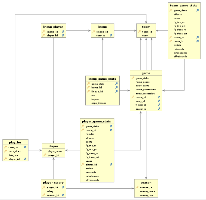
Figure 5 shows the schema of the NBA dataset. Primary key attributes are marked with a key symbol and foreign key attributes with a blue arrow on the right of an attribute’s name.
Game. Table game stores information about games including the date when the game took place (game_date), the number points scored by the home and visiting team (home_points and away_pointsw), the number of ball possessions by each team (home_possessions and away_possessions), the ids of the home, visiting, and winning team (home_id, away_id, winner_id), and the season when the team took place (season_id). Games are uniquely identified by their date and the home team.
team. Table team stores an artificial key (team_id and the name (team) of NBA teams.
player. Table player records the name (player_name) and artificial identifiers (player_id) of NBA players.
player_salary. Table player_salary stores the salary a player is earning in a particular season.
play_for. Table play_for stores which player played for which team for which time period (start_date to end_date).
line_up and lineup_player. Table lineup records lineups. Each lineup is a set of players (table lineup_player) from a team that are together on the field during a game.
team_game_stats. This table stores statistics related to the performance of a team in a particular game. The following statistics are reported. The number of points scored by the team (points), offensive possesions (offposs), number of field goals made (fg_two_m), two point field goal percentage (fg_two_pct), three point field goal made(fg_three_m), three point percentage (fg_three_pct), team assists total(assists), team total rebounds (rebounds), team defensive rebounds(defrebounds), team offensive rebounds (offrebounds). We used this simplified version of team_game_stats table in user study. In experiments we used a richer number of columns for this table and because of the space constraint we only report the list of their names here: \seqsplitfg_two_a, fg_three_a, nonheavefg_three_pct, ftpoints, ptsassisted_two_s, ptsunassisted_two_s, ptsassisted_three_s, ptsunassisted_three_s, assisted_two_spct, nonputbacksassisted_two_spct, assisted_three_spct, fg_three_apct, shotqualityavg, efgpct, tspct, ptsputbacks, fg_two_ablocked, fg_two_apctblocked, fg_three_ablocked, fg_three_apctblocked, assistpoints, two_ptassists, three_ptassists, atrimassists, shortmidrangeassists, longmidrangeassists, corner_three_assists, arc_three_assists, ftdefrebounds, defftreboundpct, def_two_ptrebounds, def_two_ptreboundpct, def_three_ptrebounds, def_three_ptreboundpct, deffgreboundpct, ftoffrebounds, offftreboundpct, off_two_ptrebounds, off_two_ptreboundpct, off_three_ptrebounds, off_three_ptreboundpct, offfgreboundpct, defatrimreboundpct, defshortmidrangereboundpct, deflongmidrangereboundpct, defarc_three_reboundpct, defcorner_three_reboundpct, offatrimreboundpct, offshortmidrangereboundpct, offlongmidrangereboundpct, offarc_three_reboundpct, offcorner_three_reboundpct
lineup_game_stats. This table stores statistics about the performance of a lineup in a game. total number of minutes the lineup played in the game (mp), total number of possessions this lineup have in the game (tmposs), total number of opponent lineup possesions in the game (oppo_tmposs).
player_game_stats. This table records statistics about a player’s performance in a game. The most of the attributes contained in this table has same names and meanings as those in team_game_stats except it has a unique attribute usage which describes what percentage of team plays a player was involved in while he was on the floor. Similarly, we used this simplified table in user study and richer version (please refer to team_game_stats for details) in the experiments.
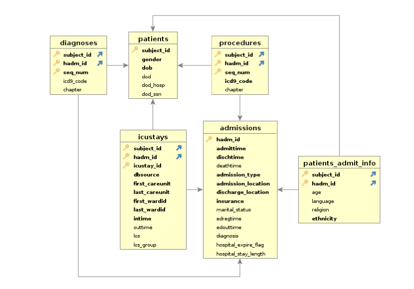
Figure 6 shows the schema of the MIMIC dataset.
admissions. This table stores information about hospital admissions. hadm_id is a unique identifier for an admission. admittime is the time when the patient got admitted. dischtime is the time when the patient was discharged from the hospital. admission_type describes the type of the admission: ELECTIVE, URGENT, NEWBORN or EMERGENCY. admission_location provides information about the previous location of the patient prior to arriving at the hospital. discharge_location provides information about the location of the patient after visiting the hospital. insurance is the type of insurance the patient has. martial_status is the patient’s martial status. edregtime is the time that the patient was registered in the emergency department edouttime is the time that the patient was discharged from the emergency department. diagnosis provides a preliminary, free text diagnosis for the patient on hospital admission hospital_expire_flag indicates whether the patient died within the given hospitalization. 1 indicates death in the hospital, and 0 indicates survival to hospital discharge. hospital_stay_length Is the length of the patient’s stay in the hospital in days.
procedures. Table procedures records information of medical procedures for each patient. seq_num is part of the primary key in procedure table to differentiating one procedure from another during one admission for the same patient. icd9_code: ICD-9 Procedure Codes to represent the procedure chapter: a broader category which contains certain icd9 codes as a group.
patients. This table records information about patients. subject_id is a unique identifier for a patient. For each patient we record their gender and date of birth (dob). dodis the date of death for the given patient. dod_hosp is the date of death as recorded in the hospital database. dod_ssn is the date of death from the social security database
patients_admit_info. This table records additional information about patients at the time of an hospital admission. For each hospital admission the patient’s age, language of choice, religion, and ethnicity are recorded.
icustays. This table records information about intensive care unit (ICU) stays of a patient during an admission. A patient may stay multiple times in ICU during an admission. dbsource: ‘carevue’ indicates the record was sourced from CareVue, while metavision indicated the record was sourced from Metavision.
first_careunit and last_careunit contain, respectively, the first and last ICU type in which the patient was cared for. first_wardid and last_wardid contain the first and last ICU unit in which the patient stayed. intime provides the date and time the patient was transferred into the ICU. outtime provides the date and time the patient was transferred out of the ICU. los is the length of the patient’s stay in intensive care. los_group is a categorized length of stay where it is divided into groups.
diagnoses. This table stores information about diagnosis for patients for a particular admission. seq_num is part of the primary key in procedure table to differentiating one diagnosis from another during one admission for the same patient. icd9_code is ICD-9 Diagnoses Codes to represent the procedure chapter a broader category which contains certain icd9 codes as a group.
Experimental setup. CaJaDE is implemented in Python (version 3.6) and runs on top of PostgreSQL (version 10.14). All experiments were run on a machine with 2 x AMD Opteron 4238 CPUs, 128GB RAM, and 4 x 1 TB 7.2K RPM HDDs in hardware RAID 5.
| Parameter | Description | Default |
| the size of the database (scale factor) | 1.0 | |
| maximum number of edges per join graph (Section 4) | 3 | |
| #attributes returned by feature selection (Section 3.1) | 3 | |
| max number of numerical attributes allowed in a pattern | 3 | |
| sample rate for LCA pattern candidate generation (Section 3.2) | 0.1 | |
| sample rate for calculating F-scores of patterns (Section 3.3) | 0.3 |
Parameters and Optimizations. Table 1 shows the parameters used in our experiments and their default values. We vary the following: (1) the size of the database; (2) the maximum number of join graph edges ; (3) sample rate for F-score ; and (4) the sample rate for pattern candidate generation ().
| Step | feature sel.: = | w/o feature sel. | |||
| 0.1 | 0.3 | 0.5 | 1.0 | ||
| Feature Selection | 84.96 | 87.39 | 86.86 | 84.80 | N/A |
| Gen. Pat. Cand. | 9.43 | 9.21 | 9.25 | 9.31 | 9.39 |
| F-score Calc. | 33.19 | 91.50 | 149.21 | 226.53 | 16749.36 |
| Materialize APTs | 21.96 | 21.29 | 20.87 | 20.47 | 20.51 |
| Refine Patterns | 15.94 | 21.10 | 22.93 | 23.69 | 128 |
| Sampling for F1 | 15.52 | 21.03 | 23.44 | N/A | N/A |
| JG Enum. | 17.57 | 17.76 | 17.59 | 17.43 | 17.77 |
| total | 214.46 | 285.19 | 346.61 | 399.07 | 17017.44 |
| Step | feature sel.: = | w/o feature sel. | |||
| 0.1 | 0.3 | 0.5 | 1.0 | ||
| Feature Selection | 19.05 | 18.96 | 19.09 | 19.05 | N/A |
| Gen. Pat. Cand. | 16.91 | 16.50 | 16.71 | 16.35 | 16.44 |
| F-score Calc. | 18.34 | 74.62 | 131.43 | 226.35 | 209.28 |
| Materialize APTs | 6.62 | 7.08 | 6.74 | 6.65 | 6.98 |
| Refine Patterns | 13.01 | 16.66 | 16.86 | 15.59 | 15.22 |
| Sampling for F1 | 6.46 | 8.80 | 9.93 | N/A | N/A |
| JG Enum. | 0.24 | 0.24 | 0.24 | 0.24 | 0.24 |
| total | 82.87 | 145.15 | 203.22 | 286.50 | 250.41 |
5.1. Feature Selection
In this set of experiments, we evaluate how feature selection affects our approach. We compare our approach without feature selection as discussed in Section 3 (Naive) against with feature selection (opt). For opt we also vary the sample rate for F-score calculation (). We measured the runtime of the individual steps of our algorithm: (i) we apply feature selection to determine which attributes to use for explanations (Feature Selection); (ii) we use the LCA method to generate candidate patterns for an APT (Gen. Pat. Cand.); (iii) we materialize APTs(Materialize APTs); (iv) we create a sample of APTs(Sampling for F1) and then calculate F-scores of patterns using this sample (F-score Calc.), (v) in the refinement step we create patterns generated over categorical attributes by adding numerical attributes (Refine Patterns). Figure 7 (Figure 7) shows the runtime breakdown for MIMIC (NBA).
5.2. Join Graph Size
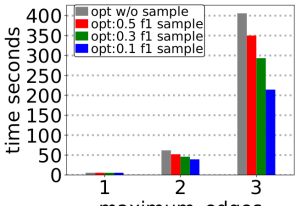
We first evaluate how the maximum number of join graphs affects performance by varying from 1 up to 3. We compare the runtime of our algorithm with feature selection varying the sample rate for F-score calculation ( = ). We use query and user question (NBA dataset) from the running example in the introduction. The results of this experiment are shown in Figure 8. As expected runtime is increases significantly in , because the number of join graphs to be considered increases dramatically when we allow for more edges per join graph. Sampling for F-score calculation improves performance by up to for when is set to 10%.
| db size | 0.1 | 0.5 | 1 | 2 | 4 | 8 |
| Feature Selection | 31.71 | 35.43 | 84.63 | 97.5 | 112.49 | 121.19 |
| Gen. Pat. Cand. | 1.25 | 2.76 | 9.18 | 16.84 | 24.92 | 42.17 |
| F-score Calc. | 12.58 | 75.99 | 174.77 | 315.31 | 635.12 | 1248.13 |
| Materialize APTs | 13.53 | 16.29 | 22 | 27.75 | 42.65 | 71.02 |
| Refine Patterns | 1.98 | 10.42 | 23.25 | 46.52 | 82.08 | 176.23 |
| Sampling for F1 | 1.11 | 8.97 | 26.98 | 51.71 | 108.59 | 203.91 |
| totals | 62.16 | 149.86 | 340.81 | 555.63 | 1005.85 | 1862.65 |
| db size | 0.1 | 0.5 | 1 | 2 | 4 | 8 |
| Feature Selection | 13.49 | 18.93 | 18.99 | 19.63 | 20.85 | 23.05 |
| Gen. Pat. Cand. | 6.4 | 15.13 | 16.46 | 19.17 | 24.6 | 34.74 |
| F-score Calc. | 15.86 | 89.63 | 161.91 | 328.08 | 611.08 | 1133.01 |
| Materialize APTs | 2.57 | 4.37 | 6.66 | 12.41 | 21.31 | 43.18 |
| Refine Patterns | 1.67 | 8.22 | 15.49 | 32.63 | 66.84 | 133.31 |
| Sampling for F1 | 1.6 | 5.58 | 11.68 | 23.91 | 51.25 | 102.16 |
| totals | 41.59 | 141.86 | 231.19 | 435.83 | 795.93 | 1469.45 |
5.3. Scalability
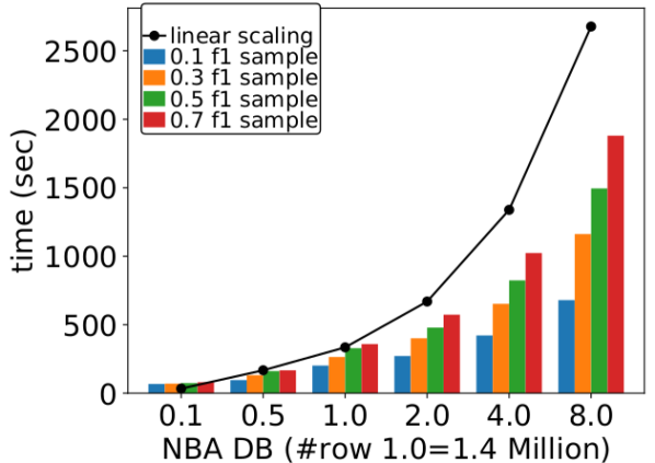
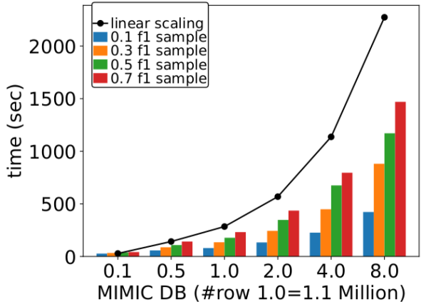
To evaluate the scalability of our approach, we use scaled versions of the NBA and MIMIC datasets ranging ( to ). We varied the F-score sample rate () from to . The results are shown in Figure 9 comparing against linear scaling (black line). The effect of database size on runtime is similar for both datasets. Our approach shows sublinear scaling for both datasets (note the log-scale x-axis). The benefits of sampling are more produced for larger database sizes: is more than 60% (70%) faster than for scale factor on the NBA (MIMIC) dataset. A detailed breakdown of the runtime of the individual steps of our algorithm for is shown in Figure 9 and Figure 9. Based on the results of our study of how sampling rate for pattern generating () affects performance and quality presented in Section 5.4 (see Figure 10 to Figure 10), we capped the number of rows sampled for LCA at . Recall that we measure the following steps of our approach: (i) we apply feature selection to determine which attributes to use for explanations (Feature Selection); (ii) we use the LCA method to generate candidate patterns for an APT (Gen. Pat. Cand.); (iii) we materialize APTs(Materialize APTs); (iv) we create a sample of APTs(Sampling for F1) and then calculate F-scores of patterns using this sample (F-score Calc.), (v) in the refinement step we create patterns generated over categorical attributes by adding numerical attributes (Refine Patterns). The major contributing factor for larger database sizes is F-score calculation which makes up than 50% of the runtime. The step with the largest growth rate is sampling for F-score calculations for the NBA dataset which is times slower for scale factor 8 compared to scale factor 0.1. Based on these results, using lower sample rates for F-score calculation is preferable for larger database sizes.
| join graph | join graph structure | APT (#rows) | # attributes |
| PT | |||
| PT - player_salary - player | |||
| PT | |||
| PT - patient_admt_info - patients |
5.4. Sample Size
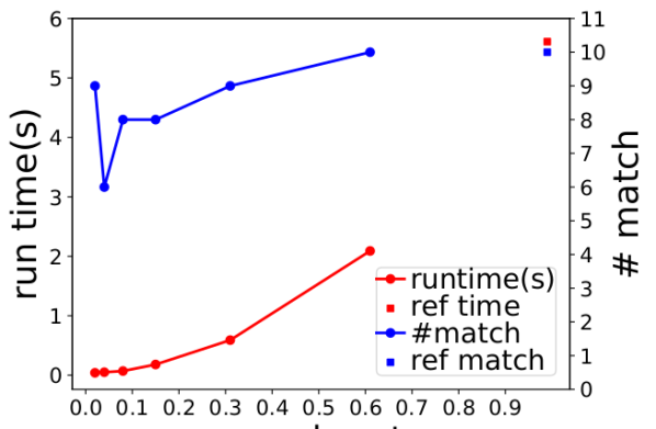
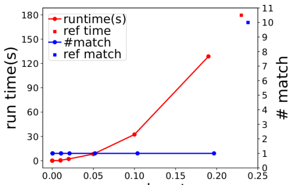
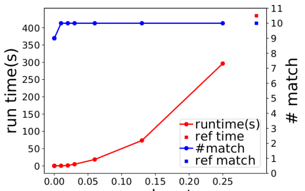
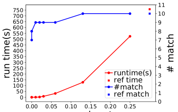
We now study the impact of sampling for F-score calculation () and for pattern candidate generation () on performance and pattern quality. We treat the result produced without sampling as ground truth and measure the difference between this result and the result produced by sampling.
Sampling for Pattern Generation. Recall that we use the LCA approach to generate candidate patterns over the categorical attributes of a database. This approach computes a cross product of a sample with itself. Our implementation of LCA ranks the pattern candidates generated by LCA by their recall, and then selects the top-k ranked patterns as input for the next step. In this experiment, we want to determine a robust choice for the LCA sample size parameter and, thus, compare the results produced by this step. We selected join graphs and their APTs: and for , and and for . Figure 10 shows the number of rows and attributes for the APTs, and join graph structure for each of these join graphs. The results are shown in Figure 10 to Figure 10. We measure pattern quality as the number of patterns from the top-10 computed over the full dataset that occur in the top-10 computed based on a sample (see the blue lines labeled match). For each materialized join graph, we also measure the runtime of generating the top-10 patterns. As expected because of the cross product computed over the sample, runtime increases quadratically in the sample size. For Figure 10 and Figure 10, all ground truth top-10 patterns are found even for just 3% sample rate. Whereas as shown in Figure 10, even for sample rate ( rows), we only find one matching pattern. The reason behind the different result observed in Figure 10 is that one of the columns in has over distinct values that are roughly evenly distributed and, thus, the recall-based ranking is sensitive to small variations in frequency caused by sampling. For fig. 10, even though this join graph also contains this attribute (over distinct values), for this APT, the column’s distribution in the APT is skewed leading to a more stable set of high frequency values that are used in the top-10 patterns. Based on these observations we determine the sample size =0.1 for the rest of the experiments and set a cap number of rows in the sample as 1000.
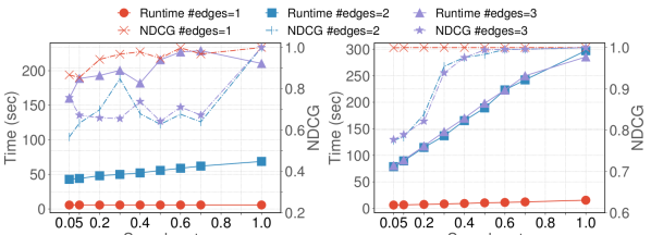
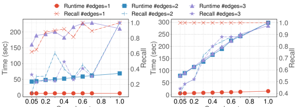
Sampling for F-score Calculation. We also use sampling to reduce the cost of the quality measure calculation (parameter ). Instead of scanning all tuples in the augmented provenance table (APT), we compute the number of matching tuples over a sample of the APT for a given pattern. Figure 10 shows the running time and the quality of patterns when varying the sample rate and maximum number of edges in join graphs () for queries and . We use the normalized discounted cumulative gain (NDCG) (Järvelin and Kekäläinen, 2002) as the sample quality metric, which is often used in information retrieval for evaluating the ranking results of recommendation and search engine algorithms. A high NDCG score (between 0 and 1) indicates that the ranking of the top patterns returned by the sampled result is close to the top patterns produced without sampling. Figure 10 shows that for both datasets for , the similarity between the sampled result and result over the full dataset is high, even for aggressive sampling. For larger join graphs (), the NDCG score fluctuates around 0.7 for the NBA dataset. For the MIMIC dataset, the NDCG converges to 1.0 at a sampling rate of 0.5. Overall, even for low sample rates, the NDCG score is at least () for the NBA (MIMIC) dataset. We also evaluate the number of patterns from sampling that are present in the results without sampling, for which we used recall as the metric as shown in Figure 10.
5.5. Comparison with Explanation Tables
We also compared our approach against the approach from (Gebaly et al., 2014) (referred to as ET from now on). We compared on one join graph with structure PT - player_game_stats - player for the NBA dataset using query and the corresponding user question from the introduction. The corresponding APT has 2600 rows and 84 columns. To be fair, we did apply our feature selection technique to filter columns for ET too, reducing the number of columns to 20. Without that step, ET took 30 seconds even for the smallest sample size (16 tuples). Figure 13 lists the runtime of CaJaDE and ET after applying feature selection. As a qualitative comparison, we list the first 20 patterns returned by ET in Section A.1. While slower for a sample size of 16 our approach scales much better when increasing the sample size ( faster for sample size 512). That being said, we would like to point out the major contribution of our work the efficient exploration of a schema graph for finding explanations. However, as this experiment demonstrates this would not be possible without our optimizations for mining patterns over a single APT.
| Runtime (sec) | ||
| Sample Size | CaJaDE | ET |
| 16 | 9.90 | 3.21 |
| 64 | 14.46 | 11.65 |
| 256 | 15.32 | 176.76 |
| 512 | 14.81 | 855.13 |
| Query | ||
| Rank | ||
| (LeBron James,-,) | (GSW,-,) | |
| (LeBron James,-,) | (GSW,-,) | |
| (LeBron James,-,) | (GSW,-,) | |
| Query | Description | Tables used |
| The average points change over the years for player Draymond Green | player, game, season, player_game_stats | |
| Team GSW average assists over the years | team_game_stats, game, team, season | |
| Average points for player Lebron James over the years | player, game, season , player_game_stats | |
| Team GSW wins over the years | team, game, season | |
| Average points by player Jimmy Butler | player, game, player_game_stats | |
| Return the number of diagnosis group by chapter(group of procedure type) | diagnoses | |
| Returns the death rate of patients grouped by their insurance. | admissions | |
| Number of ICU stays grouped by the length of stays (los_group). | icustays | |
| Number of procedures for a particular chapter (group of diagnosis types). | procedures | |
| Number admissions of different ethnicities. | patients_admit_info |
5.6. Comparison with CAPE
We compared our approach against CAPE ((Miao et al., 2019)). The question we used are from NBA running example which asks question about number of wins for GSW over the years and from the case study which asks for player LeBron James’s average points over the seasons. CAPE expects as input one data point plus a direction high or low. We select the following question for : Why was GSW number of wins high in 2015-16 season? and for : Why was LeBron James’ average points low in 2010-11 season?. Since CAPE does not explore related tables, we constructed join graphs as input to CAPE, which are PT () and PT - team_game_stats (). Figure 13 shows the top-3 explanations produced by CAPE. The system identifies a trend in the data (using regression) according to which the user question is an outlier in the user-provided direction and then returns a similar outlier in the other direction. For our experiment, this means that CAPE returns seasons with low wins for GSW and high averages points for LeBron James. This experiment demonstrates that CAPE is orthogonal to our technique. The system identifies counter-balances while we find features that are related to the difference between two query results. Nonetheless, our techniques for exploring schema graphs may be of use for finding counterbalances too.
5.7. Varying Queries
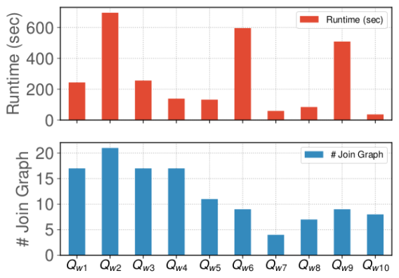
To evaluate how the runtime of our approach is affected by the choice of query, we measured the runtime for 10 different queries ( for NBA and for MIMIC) shown in Table 2. We designed these queries to access different relations and use different group-by attributes. The SQL code for these queries is shown below. All queries were run with and . The results are shown in Figure 13. We observe that the runtime is relatively stable for different queries and is to some degree correlated to the number of join graphs for the query (shown on top of Figure 13). SQL code for Query Workload. Note that the queries are based on the original schema graph which are more complex than the ones presented in the running example. The real schema can be found in Figure 6 and Figure 5.
NBA. . The average points change over the years for player Draymond Green.
. GSW average assists over the years
. Average points for Lebron James over the years
.
GSW wins over the years, but we used different 2 seasons
. Average points by Jimmy Butler over the years
MIMIC. . Return the number of diagnosis by chapter. A chapter is a type of diagnosis.
. Returns the death rate of patients grouped by their insurance.
. Number of ICU stays grouped by the length of stays (los_group).
. Number of procedures for a particular chapter (group of diagnosis types).
. Number of admits per patient ethnicity.
6. Qualitative Evaluation
We now evaluate the quality of explanations produced by CaJaDE using case studies on the same two real datasets (NBA and MIMIC) as in Section 5. We report the SQL code of queries, query results, user questions, and returned explanations for both datasets. We also report results of a user study with the NBA dataset. For both case studies, we report the top-3 explanations for each query and user question in Table 4 (NBA) and Table 6 (MIMIC). Due to the space limit, we simplified some of these descriptions. Note that the same pattern may be returned for several join graphs (same attributes, but different join path). In the interest of diversity, we removed duplicates and explanations that only differ slightly in terms of constants. We show the top-3 explanations after this step. we use “[]” or “[]” in explanations as identifier of the primary tuple for the explanation. The full sets of top-20 explanations (including join nodes and edge details) are in Section A.2.
6.1. Case Study: NBA
Setup. For the NBA dataset, we use five queries calculating player’s and team’s stats and generated user questions based on interesting results. Table 4 shows the user questions, queries, and top-3 explanations produced by our method for these user questions. Table 3 shows a description for each these queries, which include group-by aggregations over path joins. We present the SQL code for these query below. Their results and the tuples used in the user question (highlighted rows) are shown in Figure 14.
| Q | Description | Tables used |
| Average points per year for Draymond Green. | player, player_game_stats, game, season | |
| GSW average assists over the years. | team_game_stats, game, team, season | |
| Average points over the years for Lebron James . | player, player_game_stats, game, season | |
| GSW wins over the years. | game, team, season | |
| Average points over the years for Jimmy Butler. | player, player_game_stats, game, season |
| Query | User question | Top explanations | F-score |
| Draymond Green’s average points per year: 14 points in season () VS points in season () | player_salary [] | ||
| prov.tspct prov.usage salary [] | |||
| prov.minutes prov.tspct salary [] | |||
| GSW’s average assists per year: in season () VS in season () | prov.assistpoints player=Draymond Green [] | ||
| prov.assistpoints prov.nonputbackast_2_pct player.player=Harrison Barnes [] | |||
| prov.assistpoints offreboundpct [] | |||
| LeBron James’s average points per year: in season () VS in season () | player_salary [] | ||
| team=MIA [] | |||
| team=CLE [] | |||
| GSW’s number of wins per year: in () season VS in season () | player_name=Pau Gasol player_salary [] | ||
| player_name=Andre Iguodala [] | |||
| fg_3_apct team_points [] | |||
| Jimmy Butler’s average points per year: points in season () VS points in season () | player_salary [] | ||
| prov.away_points prov.efgpct [] | |||
| prov.usage team=CHI team_assisted_2_spct [] |
. The average points change over the years for player Draymond Green.
. GSW average assists over the years
. Average points for Lebron James over the years
. GSW wins over the years, but we used different 2 seasons
. Average points by Jimmy Butler over the years
| avg_pts | season_name |
| 2012-13 | |
| 2013-14 | |
| 2014-15 | |
| 2015-16 | |
| 2016-17 | |
| 2017-18 | |
| 2018-19 |
| avg_ast | season_name |
| 2009-10 | |
| 2010-11 | |
| 2011-12 | |
| 2012-13 | |
| 2013-14 | |
| 2014-15 | |
| 2015-16 | |
| 2016-17 | |
| 2017-18 | |
| 2018-19 |
| avg_pts | season_name |
| 2009-10 | |
| 2010-11 | |
| 2011-12 | |
| 2012-13 | |
| 2013-14 | |
| 2014-15 | |
| 2015-16 | |
| 2016-17 | |
| 2017-18 | |
| 2018-19 |
| avg_pts | season_name |
| 2009-10 | |
| 2010-11 | |
| 2011-12 | |
| 2012-13 | |
| 2013-14 | |
| 2014-15 | |
| 2015-16 | |
| 2016-17 | |
| 2017-18 | |
| 2018-19 |
| avg_pts | season_name |
| 2011-12 | |
| 2012-13 | |
| 2013-14 | |
| 2014-15 | |
| 2015-16 | |
| 2016-17 | |
| 2017-18 | |
| 2018-19 |
Explanations and Analysis. Draymond Green had a big average points difference between consecutive seasons. All explanation contains salary change information. In reality, from - season to - season, Green’s salary increased, which could result in losing incentive to play as hard as when he earns lower salary. and explanation successfully find key game related factors deciding the player’s points such as minutes played and shooting percentage (e.g., in , Green had more games where he played more than minutes and shooting percentage higher than in season). . The GSW team had a sudden increase in average assists. All explanations contain assistpoints which has a cause-and-effect relationship with assists (more assists result in more assistpoints). and . Both players had some significant average point changes. For , Lebron James had an average points decrease. This occurred when he switched to a new team (from CLE to MIA and had less pressure offensively in the following year. CaJaDE successfully identified this fact as a potential cause ( and ). Jimmy Butler had a big improvement in average points. Our top explanations to this improvement include an increase of usage and minutes played. . This query is similar to our running example but with a question asking for different seasons. The explanations contain player changes (, Andre Iguodala only played for GSW in season) as well as the team’s points difference and 3-point percentage (). Note that while the first explanation has a high F-score, if we look at the join graph details, the salary and player constants can have no relation with GSW at all. This highlights the importance of making join graphs part of explanations.
6.2. Case Study: MIMIC
We constructed queries over the MIMIC dataset accessing different tables. The simplified descriptions of the queries, user questions, and explanations Table 6. To help the reader understand the queries and explanations, we first briefly introduce the MIMIC dataset using the example below.
Example 0.
Consider the (simplified) MIMIC-III Critical Care database (Johnson et al., 2016) with the following relations (the keys are underlined).
-
•
Admissions(adid, dischargeloc, adtype, insurance, isdead, HospitalStayLength) contains information about hospital admissions.
-
•
Diagnoses(pid, adid, did, diagnosis, category) records the diagnoses for each patient (identified by pid) during each admission, one patient could have multiple diagnoses during one admission, which are identified by did.
-
•
PatientsAdmissionInfo(pid, admid, age, religion, ethnicity) records the information from a patient upon admission to the hospital. Note that one patient could have multiple entries in this table because one patient could have multiple admissions during their lifetime.
-
•
ICUStays(pid, admid, iid, staylength, icutype) records the information of the ICU stays of patients. iid identifies different ICU stays within one admission.
Suppose a data analyst writes the following query to find out the relationship between the insurance type and the death rate:
Given the result of this query in Figure 15(a), the analyst may ask : given similar numbers of admissions, why is the death rate of patients with insurance type= more than times larger () than that of patients with insurance=. Table 6 lists the top-3 explanations returned by CaJaDE (referred to as ), which shows that among the deaths, has a larger fraction of admissions in emergency and male older patients () compared to . This is aligned with the fact that Medicare is mostly for patients who are over years old. and are stating that patients using Medicare has more admission because of emergency and also facts about length of hospital stays.
| insurance | death rate | admit_cnt | |
| 0.14 | 28215 | ||
| Self Pay | 0.16 | 611 | |
| Government | 0.05 | 1783 | |
| 0.06 | 22582 | ||
| Medicaid | 0.07 | 5785 |
Table 5 shows a description for each these queries, which include group-by aggregations over path joins. We present the SQL code of these queries below. Their results and the tuples used in the user question (highlighted rows) are shown in Figure 16.
.
Count of diagnoses over different chapters.
User question: chapter= (neoplasms) VS chapter= (diseases of the musculoskeletal system and connective tissue)
.
Death rate of patients grouped by their insurance
User question: insurance=‘Self Pay’ VS insurance=‘Private’
.
Length of stays in ICU group by length of stays (los_group)
User question: los_group=‘’ VS los_group=‘’
.
Death rate of patients grouped by their insurance
User question: insurance=‘Medicare’ VS insurance=‘Private’
.
Number of procedures group by ethnicity
User question: ethnicity=‘ASIAN’ VS ethnicity=‘HISPANIC’
| death_rate | chapter |
| V | |
| E | |
| insurance | death rate |
| Medicare | 0.14 |
| Self Pay | 0.16 |
| Government | 0.05 |
| Private | 0.06 |
| Medicaid | 0.07 |
| cnt | los_group |
| - | |
| x | |
| - | |
| - | |
| - |
| insurance | death rate |
| Medicare | 0.14 |
| Self Pay | 0.16 |
| Government | 0.05 |
| Private | 0.06 |
| Medicaid | 0.07 |
| cnt | ethnicity |
| South American | |
| Pacific Islander | |
| Middle Eastern | |
| Multi-Race Ethnicity | |
| Declined To Answer | |
| Unable To Obtain | |
| Other | |
| Asian | |
| Hispanic | |
| Black | |
| Unkown | |
| White |
| Num. | Description | Tables used |
| Return the death rate of diagnosis by chapter | diagnoses, admissions | |
| Returns the death rate of patients grouped by their insurance. | admissions | |
| Number of ICU stays grouped by the length of stays (los_group). | icustays | |
| Number of procedures for a particular chapter (group of diagnosis types). | procedures | |
| Number of procedures among different ethnicities. | patients_admit_info, procedures |
| Query | User question | Top-3 explanations | F-score |
| Patient death rate grouped by diagnoses: for chapter () VS for chapter () | expire_flag=1 [] | ||
| hospital_stay_lengthexpire_flag [] | |||
| hospital_stay_length,expire_flag [] | |||
| Death rate by insurance: Medicare= () VS Medicaid= () | prov.admission_type=emergency [] | ||
| expire_flag [] | |||
| gender=Male [] | |||
| Number of patients grouped by ICU stays length: less than day () VS more than days () | hospital_stay_length procedure.chapter=16 [] | ||
| hospital_stay_length los_group= [] | |||
| prov.dbsource=carevue hospital_stay_length [] | |||
| Death rate by insurance: Medicare= () VS Private= () | expire_flag=age [] | ||
| prov.admission_type=emergency [] | |||
| prov.hospital_stay_length expire_flag= [] | |||
| Number of patients that did a procedure grouped by ethnicity: Hispanic patients [] VS Asian patients [] | hospital_stay_length ethnicity=Asian [] | ||
| admission_type=emergency hospital_stay_length age ethnicity=Hispanic [] | |||
| prov.religion=Catholic [] |
Explanations and Analysis. Table 6 shows the top-3 explanations for returned by CaJaDE for each user question. . This question asks for the difference in death rates between two diagnosis categories (chapter 2: neoplasms vs chapter 13: musculoskeletal system and connective tissue). The death rate is the fraction of patients that died during their hospital stay. The explanation uses expire_flag from patient table suggesting that this patient has passed away. This flag only indicates that the patient died, but not whether insides or outside the hospital, subsuming all hospital deaths. The and explanation add additional information about the lengths of hospital stays which could help user imply the severity differences between two categories thus infer the possible reason for different death rates. . This query asks about differences between the death rate of patients based on their insurance. The explanation states that there are more emergency admissions with Medicare than with Medicaid which may explain the higher death rate. The explanation related death rate to the expire_flag. The explanation suggests that Medicare has more Male patients than Medicaid. . The explanation shows that most of the patients staying over days in ICU will stay in hospital for more than days and also have procedure that is from chapter (Miscellaneous Diagnostic and Therapeutic Procedures). The and explanations are both related to the hospital stay length. The explanation suggests that most patients will be released from hospital in less than days when their ICU stay is less than day. The explanation states the same facts for patients that have more than days of hospital stay when they stay more than days in the ICU. These explanations regarding hospital stay length can help users identify that ICU stay length may be a good indicator for ICU stay lengths . This question uses the same query as , but compares Private insurance with Medicare. The explanation states that for patients who have Private insurance, more patients are alive and less than years old. This is aligned with the fact that Medicare is mostly for patients over years old (this is a fact from online resources). The and explanations are stating that patients using Medicare are more likely to be admitted because of an emergency and also facts about length of hospital stays. The explanation states that Asian patients that had a procedure are more likely to stay less than 19 days in the hospital. The explanation says that compared to Asian patients there were more Hispanic patients younger than years old and stayed more than days in the hospital. The explanation points out that more Hispanic patients are Catholic. Note that the ethnicity information appeared in explanations are not from PT, but from a different patient_admit_info table. Because we do not currently consider functional dependencies, results like this cannot be avoided. We plan to address this in future work.
6.3. User Study
We conducted a user study for the NBA dataset to evaluate: (S1) whether CaJaDE provides meaningful explanations in addition to explanations that only come from the provenance, and (S2) whether the CaJaDE’s quality metric is consistent with user preference.
Participants. We recruited 20 participants — all of them are graduate students studying in different areas of computer science, 13 of them have some prior experience with SQL, and 5 were NBA fans.
Tasks. We first presented background knowledge on the NBA to each participant, and explained the schema of the dataset. Each participant was shown the SQL query (shown below) and the results of this query, and then was asked to find and evaluate explanations for the user question from Example 1.1: “Why did win 73 games in season compared to 47 games in .”.
We gave each participant 20 minutes to explore the dataset and manually find explanations. For those unfamiliar with SQL, we skipped this step. Participants then were asked to rate each of the top-5 explanations with the highest F-scores produced based on provenance and by CaJaDE (Table 7) using a scale from 1 to 5. We also asked them which set of explanations makes more sense and whether they provided new insights. Because the top explanations by CaJaDE have higher F-scores, we added one with a low F-score () as a control. By covering a wider range of F-score values, we can test S2: (1) can participants distinguish between low and high score explanations, and (2) do participants agree with our ranking based on our quality measure.
| Provenance-based Explanations | |
| In season 2015-16, among the games GSW won, they were the visiting team and had points in 28 games (10 games in 2012-13, resp.) | |
| In 2015-16 season, 73 games (47 games in 2012-13, resp.) GSW won are regular season games. | |
| In 2015-16 season, among the games GSW won, they were the visiting team, had points and possessions in 17 games (0 games in 2012-13, resp.) | |
| In 2015-16 season, GSW scored more than 104 points in each of 64 games (24 games in 2012-13, resp.) GSW won. | |
| In 2015-16 season, the home teams had points and possessions in each of 29 games (40 games in 2012-13, resp.) GSW won. | |
| CaJaDE | |
| In 2015-16 season, the number of games with GSW player Stephen Curry’s minutes and usage is 59 games (12 games in 2012-13, resp.) GSW won. | |
| In 2015-16 season, the number of games with GSW player Draymond Green’s minutes¿15 is 73 games (15 games in 2012-13, resp.) GSW won. | |
| In 2015-16 season, Jarrett Jack played in 0 games (47 games in 2012-13, resp.) GSW won. | |
| In 2015-16 season, GSW had three_pct and points in each of 39 games (9 games in 2012-13, resp.) GSW won. | |
| In 2015-16 season, GSW had fg_three_pct and points and rebounds in 5 games (2 games in 2012-13, resp.) GSW won. | |
Results and Analysis. Overall, the responses were positive: 16 out of 20 participants agreed that explanations by CaJaDE make more sense to them and seeing explanations by CaJaDE in advance will help them find explanations that they did not think about before.
| Provenance-based | CaJaDE | |||||||||
| Expl1 | Expl2 | Expl3 | Expl4 | Expl5 | Expl6 | Expl7 | Expl8 | Expl9 | Expl10 | |
| All users | 3.150 | 1.450 | 3.950 | 3.600 | 2.750 | 3.600 | 3.800 | 2.350 | 3.950 | 2.300 |
| Stdev | 1.040 | 0.999 | 0.759 | 1.095 | 1.410 | 0.883 | 1.196 | 1.424 | 0.999 | 1.174 |
| NBA: Yes | 3.400 | 1.800 | 3.800 | 3.600 | 2.800 | 3.800 | 3.800 | 2.800 | 4.200 | 2.600 |
| NBA: No | 3.067 | 1.333 | 4.000 | 3.600 | 2.733 | 3.533 | 3.800 | 2.200 | 3.867 | 2.200 |
| F-score | 0.69 | 0.56 | 0.38 | 0.8 | 0.4 | 0.82 | 0.91 | 1 | 0.64 | 0.13 |
| recall | 0.38 | 1 | 0.23 | 0.87 | 0.4 | 0.81 | 1 | 0.99 | 0.53 | 0.07 |
| precision | 0.74 | 0.61 | 1 | 0.73 | 0.4 | 0.83 | 0.83 | 0.99 | 0.81 | 0.7 |
Table 8 shows the average user ratings and quality measures for each explanation. Regarding (S1), the average ratings of the top-1 explanation are the same for both methods ( vs , both explanations summarize the team statistics of GSW while refers to the table not in the provenance). For the next two explanations, and (CaJaDE) summarize the statistics of two GSW’s key players and have higher average ratings ( vs , vs ). The margin is larger for participants who are familiar with the NBA (4.2 vs 3.8, 3.8 vs 3.6, 3.8 vs 3.4).
To answer (S2), we find that explanations with high user ratings (Expl 3, 4 , and Expl 6, 7, 9) have a positive relation with high F-score and precision. The only exception, of CaJaDE, is also the most controversial one, indicated by the largest standard deviation. Evaluating these explanations is subjective and requires domain knowledge: the player Jack in left GSW in 2013, and people may or may not regard this as a signal that the team had begun relying more on other players who play a similar position to Jack. Next, we evaluate the ranking results of our quality measures by regarding each participant’s ratings as the ground truth. We use Kendall-Tau rank distance (Kendall, 1938) for measuring pairwise ranking error and normalized discounted cumulative gain (NDCG) (Järvelin and Kekäläinen, 2002) for the entire ranked list. As shown in Table 9, ranking by precision gives the lowest pairwise ranking error for the provenance-based method, while for our method it is ranking by F-score. If we drop the most controversial explanation, the pairwise error is reduced by more than half. The for CaJaDE reaches 0.9 for all cases and even 0.95 after dropping the most controversial explanation.
| Explanation Tables (All / -1) | CaJaDE (All / -1) | |||
| Avg. Kendall tau rank distance | All users | F-score | 3.95 / 2.2 | 3.9 / 1.4 |
| recall | 5.9 / 3.85 | 3.3 / 1.4 | ||
| precision | 2.2 / 0.95 | 3.9 / 1.4 | ||
| Users with domain knowledge | F-score | 3.6 / 2.0 | 3.2 / 1.8 | |
| recall | 5.2 / 3.2 | 3.8 / 1.8 | ||
| precision | 2.2 / 1.2 | 4.2 / 1.8 | ||
| Avg. | All users | F-score | 0.875 / 0.882 | 0.901 / 0.955 |
| recall | 0.844 / 0.852 | 0.901 / 0.955 | ||
| precision | 0.933 / 0.965 | 0.901 / 0.955 | ||
| Users with domain knowledge | F-score | 0.897 / 0.901 | 0.903 / 0.954 | |
| recall | 0.862 / 0.878 | 0.903 / 0.954 | ||
| precision | 0.953 / 0.977 | 0.903 / 0.954 | ||
Takeaways. The main findings are: (1) the majority (16/20) of participants preferred our method, thanks to the new information provided by tables not used in the query, which complements the explanations only based on provenance; (2) our quality measures are consistent with participants’ preference; (3) for both methods, there can be top explanations rated low by participants, which is as expected because we did not do causal analysis, and validating such explanations may be subjective and depend on domain expertise; and (4) participants with domain knowledge had a stronger preference for our method than participants without domain knowledge.
Other findings and discussion. Finally, it is also worth noting that the participants’ feedback supports the motivation of CaJaDE. For example, participants found that “The usage of Stephen Curry increases in 2015-16.”, “‘Players play both season (12-13 and 15-16) have higher point per game and assist per game” before they saw the explanations by CaJaDE. One suggested to use health information of the players in explanation. Another participant remarked that “the use of other tables in the database to explore how the contributions of individual players can have an outcome on the team’s performance produced explanations that were more novel or interesting”.
7. Related Work
Provenance and summarization. Provenance (Cheney et al., 2009) for relational queries refers to records of the inputs that contribute to the results of a query, which has been studied extensively. For non-aggregate queries, why-provenance (Buneman et al., 2001) returns a set of input tuples responsible for a given output tuple; how-provenance (Green et al., 2007b) encodes how the query combined input tuples to generate the answers. For aggregate queries, symbolic representation of semiring (Amsterdamer et al., 2011) is used to express how aggregate results are computed. Given the significant cost of managing provenance information in practical DBMS, different provenance-management frameworks to store and retrieve relevant provenance information have been proposed in the literature (Glavic and Alonso, 2009; Arab et al., 2014; Chapman et al., 2008; Psallidas and Wu, 2018; Lee et al., 2019). Some of them support provenance for aggregate queries using simplified models and query plan optimizations (Karvounarakis et al., 2010; Psallidas and Wu, 2018; Lee et al., 2019). A number of recent papers have proposed summarization techniques to represent provenance approximately (Ainy et al., 2015; Ré and Suciu, 2008; Lee et al., 2017, 2020), or using summarization rules for better usability (AlOmeir et al., [n. d.]). Factorized and summarized provenance in natural language (Deutch et al., 2016, 2017) has also been studied for ease of user comprehension.
Data summarization. There is a line of work on summarizing relational data where informative summarization is provided with focuses on relevance, diversity, and coverage (Qin et al., 2012; Joglekar et al., 2017; Wen et al., 2018; Kim et al., 2020). For a relation augmented with a binary outcome attribute, Gebaly et al. (Gebaly et al., 2014) developed solutions to find optimally-informative summarizations of categorical attributes affecting the outcome attribute only considering the provenance (and not other relevant relations like our work), while its extension (Vollmer et al., 2019) considers numeric data. We adopt one of the optimizations in (Gebaly et al., 2014), the use of lowest common ancestor (LCA) patterns in our algorithms to prune the search space, to generate pattern candidates from a sample to avoid the costly computation of the data cube of the sample. We discussed the potential problems in adapting the approach in (Gebaly et al., 2014) using a materialized augmented provenance table in our experiments.
Explanations for query answers. This line of work aims at explaining unexpected outcomes in a query result, including outlier values, missing tuples, or existing tuples that should not exist. Provenance and provenance summaries provide a straightforward form of explanations (Wu and Madden, 2013; Roy and Suciu, 2014; Roy et al., 2015; Abuzaid et al., 2018) by characterizing a set of tuples whose removal or modification would affect the query answer of interest; while query-based explanations, i.e., changes to queries, are investigated for “why” and “why-not” questions (Chapman and Jagadish, 2009; Bidoit et al., 2014). Explanations for outliers have been studied in (Miao et al., 2019; Bessa et al., 2020). We share with (Miao et al., 2019) the motivation of considering explanations that are not (solely) based on provenance. The difference is that in (Miao et al., 2019), the same table used in the query is considered for finding explanations that “counterbalance” an outlier by learning patterns and balancing a low (high) outlier with a high (low) outlier w.r.t. a pattern, whereas we find explanations in “augmented provenance” stemming from tables not used in the query. Therefore, (Miao et al., 2019) is orthogonal to our work.
Join path discovery. Join path discovery has been studied for finding data related to a table of interest based on inclusion dependencies or string similarity (Sarma et al., 2012; Fernandez et al., 2018; Zhu et al., 2019; He et al., 2015; Zhu et al., 2017). Recently, (Kumar et al., 2016; Shah et al., 2017; Chepurko et al., 2020) studied the performance of machine learning models trained on join results. CaJaDE can utilize join graph discovery techniques to find more augmentation opportunities.
8. Discussions and Future Work
Explanations for database query answers is a relatively new research topic with lots of interesting future directions. For instance, currently our approach only considers correlations. In the future, we plan to integrate it with existing observational causal analysis framework from AI and Statistics (Pearl, 2000; Rubin, 2005) to find causal explanations. Another interesting direction for future work is to integrate context-based explanations with join discovery techniques (e.g., (Fernandez et al., 2018; Zhu et al., 2019)) to automatically find datasets to be used as context. Finally, our approach is not suited well for textual and sparse data because such data cannot be summarized well using the type of patterns we support since values are rarely repeated. Different summarization techniques (e.g., using taxonomies) or preprocessing techniques (e.g., information extraction techniques) would have to be incorporated with our approach. While we discussed simple SQL aggregate queries, extensions of our model can be studied for more general queries (with nested sub-queries, negation) if we have access to a provenance system that can compute the query provenance. Beyond having an intuitive scoring function to rank explanations that may not always produce meaningful explanations, a challenging future work is to evaluate the correctness of provided explanations without much human interventions, to evaluate whether the returned explanations consider the intent of the user in the ‘why’ question, and to have a confidence score on the explanations by deciding whether the data has enough information to explain a user question. Finally, one can explore other types of user questions than our type of comparison question (like explaining an increasing/decreasing trend or explain why two results are similar) and applicability of context/provenance in ML applications.
References
- (1)
- Abuzaid et al. (2018) Firas Abuzaid, Peter Kraft, Sahaana Suri, Edward Gan, Eric Xu, Atul Shenoy, Asvin Ananthanarayan, John Sheu, Erik Meijer, Xi Wu, et al. 2018. DIFF: a relational interface for large-scale data explanation. Proceedings of the VLDB Endowment 12, 4 (2018), 419–432.
- Ainy et al. (2015) Eleanor Ainy, Pierre Bourhis, Susan B Davidson, Daniel Deutch, and Tova Milo. 2015. Approximated summarization of data provenance. In Proceedings of the 24th ACM International on Conference on Information and Knowledge Management. 483–492.
- AlOmeir et al. ([n. d.]) Omar AlOmeir, Eugenie Yujing Lai, Mostafa Milani, and Rachel Pottinger. [n. d.]. Summarizing Provenance of Aggregation Query Results in Relational Databases. ([n. d.]).
- Amsterdamer et al. (2011) Yael Amsterdamer, Daniel Deutch, and Val Tannen. 2011. Provenance for aggregate queries. In PODS. 153–164.
- Arab et al. (2018) Bahareh Arab, Su Feng, Boris Glavic, Seokki Lee, Xing Niu, and Qitian Zeng. 2018. GProM - A Swiss Army Knife for Your Provenance Needs. IEEE Data Engineering Bulletin 41, 1 (2018), 51–62.
- Arab et al. (2014) Bahareh Arab, Dieter Gawlick, Venkatesh Radhakrishnan, Hao Guo, and Boris Glavic. 2014. A generic provenance middleware for database queries, updates, and transactions. In TaPP.
- Barman et al. (2007) Dhiman Barman, Flip Korn, Divesh Srivastava, Dimitrios Gunopulos, Neal E. Young, and Deepak Agarwal. 2007. Parsimonious Explanations of Change in Hierarchical Data. In Proceedings of the 23rd International Conference on Data Engineering, ICDE 2007, The Marmara Hotel, Istanbul, Turkey, April 15-20, 2007, Rada Chirkova, Asuman Dogac, M. Tamer Özsu, and Timos K. Sellis (Eds.). IEEE Computer Society, 1273–1275. https://doi.org/10.1109/ICDE.2007.368991
- Bessa et al. (2020) Aline Bessa, Juliana Freire, Tamraparni Dasu, and Divesh Srivastava. 2020. Effective Discovery of Meaningful Outlier Relationships. ACM Transactions on Data Science 1, 2 (2020), 1–33.
- Bidoit et al. (2014) Nicole Bidoit, Melanie Herschel, and Katerina Tzompanaki. 2014. Query-Based Why-Not Provenance with NedExplain. In Proceedings of the 17th International Conference on Extending Database Technology, EDBT 2014, Athens, Greece, March 24-28, 2014, Sihem Amer-Yahia, Vassilis Christophides, Anastasios Kementsietsidis, Minos N. Garofalakis, Stratos Idreos, and Vincent Leroy (Eds.). OpenProceedings.org, 145–156. https://doi.org/10.5441/002/edbt.2014.14
- Breiman (2001) Leo Breiman. 2001. Random forests. Machine learning 45, 1 (2001), 5–32.
- Buneman et al. (2001) Peter Buneman, Sanjeev Khanna, and Tan Wang-Chiew. 2001. Why and where: A characterization of data provenance. In ICDT. 316–330.
- Chapman and Jagadish (2009) Adriane Chapman and HV Jagadish. 2009. Why not?. In Proceedings of the 2009 ACM SIGMOD International Conference on Management of data. 523–534.
- Chapman et al. (2008) Adriane P Chapman, Hosagrahar V Jagadish, and Prakash Ramanan. 2008. Efficient provenance storage. In Proceedings of the 2008 ACM SIGMOD international conference on Management of data. 993–1006.
- Cheney et al. (2009) James Cheney, Laura Chiticariu, and Wang Chiew Tan. 2009. Provenance in Databases: Why, How, and Where. Found. Trends Databases 1, 4 (2009), 379–474.
- Chepurko et al. (2020) Nadiia Chepurko, Ryan Marcus, Emanuel Zgraggen, Raul Castro Fernandez, Tim Kraska, and David Karger. 2020. ARDA: Automatic Relational Data Augmentation for Machine Learning. PVLDB 13, 9 (2020), 1373–1387.
- Deutch et al. (2016) Daniel Deutch, Nave Frost, and Amir Gilad. 2016. Nlprov: Natural language provenance. Proceedings of the VLDB Endowment 9, 13 (2016), 1537–1540.
- Deutch et al. (2017) Daniel Deutch, Nave Frost, and Amir Gilad. 2017. Provenance for natural language queries. Proceedings of the VLDB Endowment 10, 5 (2017), 577–588.
- Fernandez et al. (2018) Raul Castro Fernandez, Ziawasch Abedjan, Famien Koko, Gina Yuan, Samuel Madden, and Michael Stonebraker. 2018. Aurum: A Data Discovery System. In ICDE. 1001–1012.
- Gebaly et al. (2014) Kareem El Gebaly, Parag Agrawal, Lukasz Golab, Flip Korn, and Divesh Srivastava. 2014. Interpretable and Informative Explanations of Outcomes. Proc. VLDB Endow. 8, 1 (2014), 61–72. https://doi.org/10.14778/2735461.2735467
- Glavic and Alonso (2009) Boris Glavic and Gustavo Alonso. 2009. Perm: Processing provenance and data on the same data model through query rewriting. In ICDE. 174–185.
- Green et al. (2007a) Todd J. Green, Grigoris Karvounarakis, and Val Tannen. 2007a. Provenance semirings. In PODS. 31–40.
- Green et al. (2007b) Todd J Green, Grigoris Karvounarakis, and Val Tannen. 2007b. Provenance semirings. In PODS. 31–40.
- He et al. (2015) Yeye He, Kris Ganjam, and Xu Chu. 2015. SEMA-JOIN: Joining Semantically-Related Tables Using Big Table Corpora. Proc. VLDB Endow. 8, 12 (2015), 1358–1369. https://doi.org/10.14778/2824032.2824036
- Järvelin and Kekäläinen (2002) Kalervo Järvelin and Jaana Kekäläinen. 2002. Cumulated gain-based evaluation of IR techniques. ACM Transactions on Information Systems (TOIS) 20, 4 (2002), 422–446.
- Joglekar et al. (2017) Manas Joglekar, Hector Garcia-Molina, and Aditya Parameswaran. 2017. Interactive data exploration with smart drill-down. IEEE Transactions on Knowledge and Data Engineering 31, 1 (2017), 46–60.
- Johnson et al. (2016) Alistair EW Johnson, Tom J Pollard, Lu Shen, H Lehman Li-Wei, Mengling Feng, Mohammad Ghassemi, Benjamin Moody, Peter Szolovits, Leo Anthony Celi, and Roger G Mark. 2016. MIMIC-III, a freely accessible critical care database. Scientific data 3, 1 (2016), 1–9.
- Karvounarakis et al. (2010) Grigoris Karvounarakis, Zachary G Ives, and Val Tannen. 2010. Querying data provenance. In Proceedings of the 2010 ACM SIGMOD International Conference on Management of data. 951–962.
- Kendall (1938) Maurice G Kendall. 1938. A new measure of rank correlation. Biometrika 30, 1/2 (1938), 81–93.
- Kim et al. (2020) Alexandra Kim, Laks VS Lakshmanan, and Divesh Srivastava. 2020. Summarizing Hierarchical Multidimensional Data. In 2020 IEEE 36th International Conference on Data Engineering (ICDE). IEEE, 877–888.
- Kumar et al. (2016) Arun Kumar, Jeffrey F. Naughton, Jignesh M. Patel, and Xiaojin Zhu. 2016. To Join or Not to Join?: Thinking Twice about Joins before Feature Selection. In SIGMOD, Fatma Özcan, Georgia Koutrika, and Sam Madden (Eds.). ACM, 19–34.
- Lee et al. (2019) Seokki Lee, Bertram Ludäscher, and Boris Glavic. 2019. PUG: a framework and practical implementation for why and why-not provenance. The VLDB Journal 28, 1 (2019), 47–71.
- Lee et al. (2020) Seokki Lee, Bertram Ludäscher, and Boris Glavic. 2020. Approximate Summaries for Why and Why-not Provenance. PVLDB 13, 6 (2020), 912–924.
- Lee et al. (2017) Seokki Lee, Xing Niu, Bertram Ludäscher, and Boris Glavic. 2017. Integrating approximate summarization with provenance capture. In 9th USENIX Workshop on the Theory and Practice of Provenance (TaPP 2017).
- Miao et al. (2019) Zhengjie Miao, Qitian Zeng, Boris Glavic, and Sudeepa Roy. 2019. Going Beyond Provenance: Explaining Query Answers with Pattern-based Counterbalances. In Proceedings of the 2019 International Conference on Management of Data, SIGMOD Conference 2019, Amsterdam, The Netherlands, June 30 - July 5, 2019, Peter A. Boncz, Stefan Manegold, Anastasia Ailamaki, Amol Deshpande, and Tim Kraska (Eds.). ACM, 485–502. https://doi.org/10.1145/3299869.3300066
- NBA.com (2020) NBA.com. 2020. The official site of the NBA. https://www.nba.com/
- Pearl (2000) Judea Pearl. 2000. Causality: models, reasoning, and inference. Cambridge University Press.
- Psallidas and Wu (2018) Fotis Psallidas and Eugene Wu. 2018. Smoke: Fine-grained lineage at interactive speed. PVLDB 11, 6 (2018), 719–732.
- Qin et al. (2012) Lu Qin, Jeffrey Xu Yu, and Lijun Chang. 2012. Diversifying Top-K Results. Proc. VLDB Endow. 5, 11 (2012), 1124–1135. https://doi.org/10.14778/2350229.2350233
- Ré and Suciu (2008) Christopher Ré and Dan Suciu. 2008. Approximate lineage for probabilistic databases. Proceedings of the VLDB Endowment 1, 1 (2008), 797–808.
- Roweis and Saul (2000) Sam T Roweis and Lawrence K Saul. 2000. Nonlinear dimensionality reduction by locally linear embedding. Science 290, 5500 (2000), 2323–2326.
- Roy et al. (2015) Sudeepa Roy, Laurel Orr, and Dan Suciu. 2015. Explaining query answers with explanation-ready databases. PVLDB 9, 4 (2015), 348–359.
- Roy and Suciu (2014) Sudeepa Roy and Dan Suciu. 2014. A formal approach to finding explanations for database queries. SIGMOD.
- Rubin (2005) Donald B Rubin. 2005. Causal inference using potential outcomes: Design, modeling, decisions. J. Amer. Statist. Assoc. 100, 469 (2005), 322–331.
- Sarle (1990) WS Sarle. 1990. SAS/STAT User’s Guide: The VARCLUS Procedure. SAS Institute, Inc., Cary, NC, USA, (1990), 134.
- Sarma et al. (2012) Anish Das Sarma, Lujun Fang, Nitin Gupta, Alon Y. Halevy, Hongrae Lee, Fei Wu, Reynold Xin, and Cong Yu. 2012. Finding related tables. In SIGMOD. 817–828.
- Shah et al. (2017) Vraj Shah, Arun Kumar, and Xiaojin Zhu. 2017. Are Key-Foreign Key Joins Safe to Avoid when Learning High-Capacity Classifiers? PVLDB 11, 3 (2017), 366–379.
- ten Cate et al. (2015) Balder ten Cate, Cristina Civili, Evgeny Sherkhonov, and Wang-Chiew Tan. 2015. High-Level Why-Not Explanations using Ontologies. In Proceedings of the 34th ACM Symposium on Principles of Database Systems, PODS 2015, Melbourne, Victoria, Australia, May 31 - June 4, 2015, Tova Milo and Diego Calvanese (Eds.). ACM, 31–43. https://doi.org/10.1145/2745754.2745765
- Vardi (1982) Moshe Y. Vardi. 1982. The Complexity of Relational Query Languages (Extended Abstract). In Proceedings of the Fourteenth Annual ACM Symposium on Theory of Computing (STOC ’82). ACM, New York, NY, USA, 137–146. https://doi.org/10.1145/800070.802186
- Vollmer et al. (2019) Michael Vollmer, Lukasz Golab, Klemens Böhm, and Divesh Srivastava. 2019. Informative Summarization of Numeric Data. In SSDBM. 97–108.
- Wang and Meliou (2019) Xiaolan Wang and Alexandra Meliou. 2019. Explain3D: Explaining Disagreements in Disjoint Datasets. Proc. VLDB Endow. 12, 7 (2019), 779–792. https://doi.org/10.14778/3317315.3317320
- Wen et al. (2018) Yuhao Wen, Xiaodan Zhu, Sudeepa Roy, and Jun Yang. 2018. Interactive summarization and exploration of top aggregate query answers. In Proceedings of the VLDB Endowment. International Conference on Very Large Data Bases, Vol. 11. NIH Public Access, 2196.
- Wu and Madden (2013) Eugene Wu and Samuel Madden. 2013. Scorpion: Explaining Away Outliers in Aggregate Queries. PVLDB 6, 8 (2013), 553–564.
- Zhu et al. (2019) Erkang Zhu, Dong Deng, Fatemeh Nargesian, and Renée J. Miller. 2019. JOSIE: Overlap Set Similarity Search for Finding Joinable Tables in Data Lakes. In SIGMOD. 847–864.
- Zhu et al. (2017) Erkang Zhu, Yeye He, and Surajit Chaudhuri. 2017. Auto-Join: Joining Tables by Leveraging Transformations. Proc. VLDB Endow. 10, 10 (2017), 1034–1045. https://doi.org/10.14778/3115404.3115409
Appendix A Appendix
A.1. Top 20 patterns returned by Explanation Table
Note since ET doesn’t accept numeric attributes, we did a preprocessing step by converting numeric values into categorical value. As shown in Table 10, the large number of predicates make the results hard comprehend. Plus, since ET is mainly focused on maximizing information gain, the result should be interpreted as a set, which make the result even harder to understand.
| Num | Pattern Description |
| Pattern 1 | fg_three_pct[] off_three_ptreboundpct[] |
| Pattern 2 | off_three_ptreboundpct[] |
| Pattern 3 | rebounds[] off_three_ptreboundpct[] |
| Pattern 4 | fg_three_pct[] three_ptassists[] fg_three_apct[] fg_two_ablocked[] |
| Pattern 5 | offfgreboundpct[] prov_game_away__points[] three_ptassists[] |
| Pattern 6 | prov_game_away__points[] fg_two_ablocked[] |
| Pattern 7 | assistpoints[] rebounds[] player_nameDraymond Green |
| Pattern 8 | minutes[] fg_three_apct[] |
| Pattern 9 | offfgreboundpct[] minutes[] assisted_two_spct[] def_three_ptreboundpct[] offftreboundpct[] |
| Pattern 10 | off_three_ptreboundpct[] shotqualityavg[] fg_two_ablocked[] |
| Pattern 11 | fg_three_pct[] tspct[] defftreboundpct[] |
| Pattern 12 | assisted_two_spct[] def_three_ptreboundpct[] offftreboundpct[] fg_three_apct[] usage[] |
| Pattern 13 | off_three_ptreboundpct[] tspct[] defftreboundpct[] three_ptassists[] fg_three_apct[] shotqualityavg[] |
| Pattern 14 | assistpoints[] fg_three_pct[] minutes[] prov_game_away__points[] tspct[] defftreboundpct[] |
| Pattern 15 | rebounds[] fg_three_pct[] shotqualityavg[] |
| Pattern 16 | assistpoints[] assisted_two_spct[] fg_two_ablocked[] usage[] |
| Pattern 17 | offfgreboundpct[] prov_game_away__points[] usage[] |
| Pattern 18 | assistpoints[] off_three_ptreboundpct[] assisted_two_spct[] tspct[] |
| Pattern 19 | assistpoints[] player_nameJarrett Jack |
| Pattern 20 | prov_game_away__points[] fg_two_ablocked[] |
| Nodes | Edges | Pattern Desc | Precision | Recall | F-score | Primary Tuple |
| : PT : team : player_salary | (.team_id)=(.prov_game_away__id) (.prov_player_player__id)=(.player_id) (.prov_season_season__id)=(.season_id) | .prov_season_season__type=regular season .salary¡15330435.0 | 1.0 | 1.0 | 1.0 | 2015-16 |
| : PT : team : player_salary | (.team_id)=(.prov_game_winner__id) (.prov_player_player__id)=(.player_id) (.prov_season_season__id)=(.season_id) | .prov_season_season__type=regular season .salary¡15330435.0 | 1.0 | 1.0 | 1.0 | 2015-16 |
| : PT : team : player_salary | (.team_id)=(.prov_game_home__id) (.prov_player_player__id)=(.player_id) (.prov_season_season__id)=(.season_id) | .prov_season_season__type=regular season .salary¡15330435.0 | 1.0 | 1.0 | 1.0 | 2015-16 |
| : PT : team : player_salary | (.team_id)=(.prov_game_away__id) (.prov_player_player__id)=(.player_id) (.prov_season_season__id)=(.season_id) | .prov_player__game__stats_tspct¡0.69 .prov_player__game__stats_usage¡20.51 .prov_season_season__type=regular season .salary¿14260870.0 | 1.0 | 0.71 | 0.83 | 2016-17 |
| : PT : team : player_salary | (.team_id)=(.prov_game_home__id) (.prov_player_player__id)=(.player_id) (.prov_season_season__id)=(.season_id) | .prov_player__game__stats_tspct¡0.69 .prov_player__game__stats_usage¡20.51 .prov_season_season__type=regular season .salary¿14260870.0 | 1.0 | 0.71 | 0.83 | 2016-17 |
| : PT : team : player_salary | (.team_id)=(.prov_game_winner__id) (.prov_player_player__id)=(.player_id) (.prov_season_season__id)=(.season_id) | .prov_player__game__stats_tspct¡0.69 .prov_player__game__stats_usage¡20.51 .prov_season_season__type=regular season .salary¿14260870.0 | 1.0 | 0.71 | 0.83 | 2016-17 |
| : PT : team : player_salary | (.team_id)=(.prov_game_winner__id) (.prov_player_player__id)=(.player_id) (.prov_season_season__id)=(.season_id) | .prov_player__game__stats_minutes¿30.7 .prov_player__game__stats_tspct¿0.42 .prov_season_season__type=regular season .salary¡15330435.0 | 1.0 | 0.69 | 0.82 | 2015-16 |
| : PT : team : player_salary | (.team_id)=(.prov_game_away__id) (.prov_player_player__id)=(.player_id) (.prov_season_season__id)=(.season_id) | .prov_player__game__stats_minutes¿30.7 .prov_player__game__stats_tspct¿0.42 .prov_season_season__type=regular season .salary¡15330435.0 | 1.0 | 0.69 | 0.82 | 2015-16 |
| : PT : team : player_salary | (.team_id)=(.prov_game_home__id) (.prov_player_player__id)=(.player_id) (.prov_season_season__id)=(.season_id) | .prov_player__game__stats_tspct¿0.42 .prov_player__game__stats_usage¿14.06 .prov_season_season__type=regular season .salary¡15330435.0 | 1.0 | 0.67 | 0.8 | 2015-16 |
| : PT : team : player_salary | (.team_id)=(.prov_game_winner__id) (.prov_player_player__id)=(.player_id) (.prov_season_season__id)=(.season_id) | .prov_player__game__stats_tspct¿0.42 .prov_player__game__stats_usage¿14.02 .prov_season_season__type=regular season .salary¡15330435.0 .team=GSW | 1.0 | 0.59 | 0.74 | 2015-16 |
| : PT : team : player_salary | (.team_id)=(.prov_game_winner__id) (.prov_player_player__id)=(.player_id) (.prov_season_season__id)=(.season_id) | .prov_player__game__stats_minutes¡36.105 .prov_player__game__stats_usage¡20.21 .prov_season_season__type=regular season .salary¿14260870.0 .team=GSW | 1.0 | 0.59 | 0.74 | 2016-17 |
| : PT : team : player_salary | (.team_id)=(.prov_game_home__id) (.prov_player_player__id)=(.player_id) (.prov_season_season__id)=(.season_id) | .prov_player__game__stats_minutes¡36.57 .prov_player__game__stats_usage¿14.06 .prov_season_season__type=regular season .salary¿14260870.0 | 1.0 | 0.59 | 0.74 | 2016-17 |
| : PT : team | (.team_id)=(.prov_game_away__id) (.team_id)=(.prov_game_winner__id) | .prov_player__game__stats_fg__three__apct¡0.4875 .prov_season_season__type=regular season .team=GSW | 0.65 | 0.83 | 0.73 | 2015-16 |
| : PT : team : team_game_stats : team | (.team_id)=(.prov_game_home__id) (.prov_game_game__date)=(.game_date) (.prov_game_home__id)=(.home_id) (.team_id)=(.team_id) | .prov_player__game__stats_deflongmidrangereboundpct¿0.1 .prov_season_season__type=regular season .team=GSW | 0.59 | 0.84 | 0.69 | 2015-16 |
| : PT : team : team_game_stats : team | (.team_id)=(.prov_game_away__id) (.prov_game_game__date)=(.game_date) (.prov_game_home__id)=(.home_id) (.team_id)=(.team_id) | .prov_player__game__stats_deflongmidrangereboundpct¿0.1 .prov_season_season__type=regular season .team=GSW | 0.59 | 0.84 | 0.69 | 2015-16 |
| : PT : team : team_game_stats : team | (.team_id)=(.prov_game_winner__id) (.prov_game_game__date)=(.game_date) (.prov_game_home__id)=(.home_id) (.team_id)=(.team_id) | .prov_player__game__stats_deflongmidrangereboundpct¿0.1 .prov_season_season__type=regular season .team=GSW | 0.59 | 0.84 | 0.69 | 2015-16 |
| : PT : team : play_for : team | (.team_id)=(.prov_game_away__id) (.prov_player_player__id)=(.player_id) (.team_id)=(.team_id) | .prov_player__game__stats_minutes¿30.7 .prov_season_season__type=regular season .date_end=2019-04-09 .team=GSW | 0.58 | 0.84 | 0.69 | 2015-16 |
| : PT : team : play_for : team | (.team_id)=(.prov_game_home__id) (.prov_player_player__id)=(.player_id) (.team_id)=(.team_id) | .prov_player__game__stats_minutes¿30.7 .prov_season_season__type=regular season .date_end=2019-04-09 .team=GSW | 0.58 | 0.84 | 0.69 | 2015-16 |
| : PT : team : play_for : team | (.team_id)=(.prov_game_winner__id) (.prov_player_player__id)=(.player_id) (.team_id)=(.team_id) | .prov_player__game__stats_minutes¿30.7 .prov_season_season__type=regular season .date_end=2019-04-09 .team=GSW | 0.58 | 0.84 | 0.69 | 2015-16 |
| A_1 | .prov_player__game__stats_minutes¿30.7 .prov_season_season__type=regular season | 0.58 | 0.84 | 0.69 | 2015-16 |
| Nodes | Edges | Pattern Desc | Precision | Recall | F-score | Primary Tuple |
| : PT : team : player_game_stats : player | (.team_id)=(.prov_game_away__id) (.prov_game_game__date)=(.game_date) (.prov_game_home__id)=(.home_id) (.player_id)=(.player_id) | .prov_season_season__type=regular season .prov_team__game__stats_assistpoints¡68.0 .player_name=Draymond Green | 0.62 | 0.9 | 0.74 | 2013-14 |
| : PT : team : player_game_stats : player | (.team_id)=(.prov_game_winner__id) (.prov_game_game__date)=(.game_date) (.prov_game_home__id)=(.home_id) (.player_id)=(.player_id) | .prov_season_season__type=regular season .prov_team__game__stats_assistpoints¡68.0 .player_name=Draymond Green | 0.62 | 0.9 | 0.74 | 2013-14 |
| : PT : team : player_game_stats : player | (.team_id)=(.prov_game_home__id) (.prov_game_game__date)=(.game_date) (.prov_game_home__id)=(.home_id) (.player_id)=(.player_id) | .prov_season_season__type=regular season .prov_team__game__stats_assistpoints¡68.0 .player_name=Draymond Green | 0.62 | 0.9 | 0.74 | 2013-14 |
| : PT : team : player_game_stats : player | (.team_id)=(.prov_game_winner__id) (.prov_game_game__date)=(.game_date) (.prov_game_home__id)=(.home_id) (.player_id)=(.player_id) | .prov_season_season__type=regular season .prov_team__game__stats_assistpoints¿57.0 .prov_team__game__stats_nonputback- sassisted__two__spct¿0.55 .player_name=Harrison Barnes | 0.78 | 0.7 | 0.74 | 2014-15 |
| : PT : team : player_game_stats : player | (.team_id)=(.prov_game_home__id) (.prov_game_game__date)=(.game_date) (.prov_game_home__id)=(.home_id) (.player_id)=(.player_id) | .prov_season_season__type=regular season .prov_team__game__stats_assistpoints¿57.0 .prov_team__game__stats_nonputbacksassisted__two__spct¿0.5475 .player_name=Harrison Barnes | 0.78 | 0.7 | 0.74 | 2014-15 |
| : PT : team : player_salary : player | (.team_id)=(.prov_game_winner__id) (.prov_season_season__id)=(.season_id) (.player_id)=(.player_id) | .prov_season_season__type=regular season .prov_team__game__stats_assistpoints¡68.0 .player_name=Gal Mekel | 0.61 | 0.9 | 0.73 | 2013-14 |
| A_1 | .prov_season_season__type=regular season .prov_team__game__stats_assistpoints¡68.0 | 0.61 | 0.9 | 0.73 | 2013-14 | |
| A_1 | .prov_season_season__type=regular season .prov_team__game__stats_assistpoints¡68.0 .prov_team__game__stats_offatrimreboundpct¿0.25 | 0.71 | 0.72 | 0.72 | 2013-14 | |
| : PT : team : player_game_stats : player | (.team_id)=(.prov_game_away__id) (.prov_game_game__date)=(.game_date) (.prov_game_home__id)=(.home_id) (.player_id)=(.player_id) | .prov_season_season__type=regular season .prov_team__game__stats_assistpoints¡67.0 .prov_team__game__stats_nonputbacksassisted__two__spct¡0.69 .player_name=David Lee | 0.75 | 0.67 | 0.71 | 2013-14 |
| : PT : team : player_salary : player | (.team_id)=(.prov_game_winner__id) (.prov_season_season__id)=(.season_id) (.player_id)=(.player_id) | .prov_season_season__type=regular season .prov_team__game__stats_assistpoints¿58.5 .prov_team__game__stats_nonputbacksassisted__two__spct¿0.55 .player_name=Mike Muscala | 0.74 | 0.68 | 0.71 | 2014-15 |
| : PT : team : player_game_stats : player | (.team_id)=(.prov_game_home__id) (.prov_game_game__date)=(.game_date) (.prov_game_home__id)=(.home_id) (.player_id)=(.player_id) | .prov_season_season__type=regular season .prov_team__game__stats_assistpoints¿50.0 .prov_team__game__stats_nonputbacksassisted__two__spct¿0.5525 .player_name=Stephen Curry | 0.65 | 0.78 | 0.71 | 2014-15 |
| : PT : team | (.team_id)=(.prov_game_home__id) (.team_id)=(.prov_game_winner__id) | .prov_season_season__type=regular season .prov_team__game__stats_assistpoints¿57.0 .team=GSW | 0.72 | 0.65 | 0.69 | 2014-15 |
| : PT : team | (.team_id)=(.prov_game_away__id) (.team_id)=(.prov_game_winner__id) | .prov_season_season__type=regular season .team=GSW | 0.54 | 0.93 | 0.68 | 2014-15 |
| : PT : team : player_game_stats : player | (.team_id)=(.prov_game_winner__id) (.prov_game_game__date)=(.game_date) (.prov_game_home__id)=(.home_id) (.player_id)=(.player_id) | .prov_season_season__type=regular season .prov_team__game__stats_assistpoints¿50.0 .prov_team__game__stats_nonputbacksassisted__two__spct¿0.55 .player_name=Marreese Speights | 0.63 | 0.73 | 0.68 | 2014-15 |
| : PT : team : player_game_stats : player | (.team_id)=(.prov_game_home__id) (.prov_game_game__date)=(.game_date) (.prov_game_home__id)=(.home_id) (.player_id)=(.player_id) | .prov_season_season__type=regular season .prov_team__game__stats_nonputbacksassisted__two__spct¡0.68 .prov_team__game__stats_offatrimreboundpct¿0.25 .player_name=Klay Thompson | 0.71 | 0.65 | 0.68 | 2013-14 |
| : PT : team : player_game_stats : player | (.team_id)=(.prov_game_away__id) (.prov_game_game__date)=(.game_date) (.prov_game_home__id)=(.home_id) (.player_id)=(.player_id) | .prov_season_season__type=regular season .prov_team__game__stats_nonputbacksassisted__two__spct¡0.68 .prov_team__game__stats_offatrimreboundpct¿0.25 .player_name=Klay Thompson | 0.71 | 0.65 | 0.68 | 2013-14 |
| : PT : team | (.team_id)=(.prov_game_winner__id) | .prov_season_season__type=regular season .team=GSW | 0.57 | 0.82 | 0.67 | 2014-15 |
| : PT : team : player_salary : player | (.team_id)=(.prov_game_winner__id) (.prov_season_season__id)=(.season_id) (.player_id)=(.player_id) | .prov_season_season__type=regular season .prov_team__game__stats_nonputbacksassisted__two__spct¡0.69 .prov_team__game__stats_offatrimreboundpct¿0.25 .player_name=Gal Mekel | 0.65 | 0.67 | 0.66 | 2013-14 |
| A_1 | .prov_season_season__type=regular season .prov_team__game__stats_assisted__three__spct¿0.6975 .prov_team__game__stats_assistpoints¿58.5 | 0.71 | 0.62 | 0.66 | 2014-15 | |
| : PT : team | (.team_id)=(.prov_game_home__id) (.team_id)=(.prov_game_winner__id) | .prov_season_season__type=regular season .prov_team__game__stats_assistpoints¿57.0 .prov_team__game__stats_nonputbacksassisted__two__spct¿0.59 .team=GSW | 0.77 | 0.58 | 0.66 | 2014-15 |
| Nodes | Edges | Pattern Desc | Precision | Recall | F-score | Primary Tuple |
| : PT : team : player_salary | (.team_id)=(.prov_game_away__id) (.prov_player_player__id)=(.player_id) (.prov_season_season__id)=(.season_id) | .prov_season_season__type=regular season .salary¿14500000.0 | 1.0 | 1.0 | 1.0 | 2009-10 |
| : PT : team : player_salary | (.team_id)=(.prov_game_winner__id) (.prov_player_player__id)=(.player_id) (.prov_season_season__id)=(.season_id) | .prov_season_season__type=regular season .salary¿14500000.0 | 1.0 | 1.0 | 1.0 | 2009-10 |
| : PT : team : player_salary | (.team_id)=(.prov_game_home__id) (.prov_player_player__id)=(.player_id) (.prov_season_season__id)=(.season_id) | .prov_season_season__type=regular season .salary¿14500000.0 | 1.0 | 1.0 | 1.0 | 2009-10 |
| : PT : team : team_game_stats : team | (.team_id)=(.prov_game_away__id) (.prov_game_game__date)=(.game_date) (.prov_game_home__id)=(.home_id) (.team_id)=(.team_id) | .prov_season_season__type=regular season .team=MIA | 0.96 | 1.0 | 0.98 | 2010-11 |
| : PT : team : team_game_stats : team | (.team_id)=(.prov_game_home__id) (.prov_game_game__date)=(.game_date) (.prov_game_home__id)=(.home_id) (.team_id)=(.team_id) | .prov_season_season__type=regular season .team=MIA | 0.96 | 1.0 | 0.98 | 2010-11 |
| : PT : team : team_game_stats : team | (.team_id)=(.prov_game_winner__id) (.prov_game_game__date)=(.game_date) (.prov_game_home__id)=(.home_id) (.team_id)=(.team_id) | .prov_season_season__type=regular season .team=MIA | 0.96 | 1.0 | 0.98 | 2010-11 |
| : PT : team | (.team_id)=(.prov_game_away__id) (.team_id)=(.prov_game_winner__id) | .prov_season_season__type=regular season .team=CLE | 1.0 | 0.87 | 0.93 | 2009-10 |
| : PT : team | (.team_id)=(.prov_game_winner__id) | .prov_season_season__type=regular season .team=CLE | 0.98 | 0.79 | 0.88 | 2009-10 |
| : PT : team : play_for : team | (.team_id)=(.prov_game_winner__id) (.prov_player_player__id)=(.player_id) (.team_id)=(.team_id) | .prov_season_season__type=regular season .date_end=2018-04-11 .team=CLE .team=CLE | 0.98 | 0.79 | 0.88 | 2009-10 |
| : PT : team | (.team_id)=(.prov_game_home__id) (.team_id)=(.prov_game_winner__id) | .prov_season_season__type=regular season .team=MIA | 1.0 | 0.73 | 0.85 | 2010-11 |
| : PT : team : player_salary | (.team_id)=(.prov_game_winner__id) (.prov_player_player__id)=(.player_id) (.prov_season_season__id)=(.season_id) | .prov_player__game__stats_assisted__two__spct¿0.19 .prov_player__game__stats_usage¿28.025 .prov_season_season__type=regular season .salary¿14500000.0 | 1.0 | 0.71 | 0.83 | 2009-10 |
| : PT : team : player_salary | (.team_id)=(.prov_game_away__id) (.prov_player_player__id)=(.player_id) (.prov_season_season__id)=(.season_id) | .prov_player__game__stats_assisted__two__spct¿0.19 .prov_player__game__stats_usage¿28.025 .prov_season_season__type=regular season .salary¿14500000.0 | 1.0 | 0.71 | 0.83 | 2009-10 |
| : PT : team : player_salary | (.team_id)=(.prov_game_home__id) (.prov_player_player__id)=(.player_id) (.prov_season_season__id)=(.season_id) | .prov_player__game__stats_deflongmidrangereboundpct¿0.1 .prov_player__game__stats_usage¿28.025 .prov_season_season__type=regular season .salary¿14500000.0 | 1.0 | 0.7 | 0.82 | 2009-10 |
| : PT : team : player_salary | (.team_id)=(.prov_game_away__id) (.prov_player_player__id)=(.player_id) (.prov_season_season__id)=(.season_id) | .prov_player__game__stats_assisted__two__spct¡0.5 .prov_player__game__stats_def__three__ptreboundpct¡0.25 .prov_season_season__type=regular season .salary¡15779912.0 | 1.0 | 0.65 | 0.78 | 2010-11 |
| : PT : team : player_salary | (.team_id)=(.prov_game_winner__id) (.prov_player_player__id)=(.player_id) (.prov_season_season__id)=(.season_id) | .prov_player__game__stats_assisted__two__spct¡0.5 .prov_player__game__stats_def__three__ptreboundpct¡0.25 .prov_season_season__type=regular season .salary¡15779912.0 | 1.0 | 0.65 | 0.78 | 2010-11 |
| : PT : team : player_salary | (.team_id)=(.prov_game_home__id) (.prov_player_player__id)=(.player_id) (.prov_season_season__id)=(.season_id) | .prov_player__game__stats_assisted__two__spct¡0.5 .prov_player__game__stats_usage¡36.36 .prov_season_season__type=regular season .salary¡15779912.0 | 1.0 | 0.63 | 0.78 | 2010-11 |
| : PT : team : player_salary | (.team_id)=(.prov_game_home__id) (.prov_player_player__id)=(.player_id) (.prov_season_season__id)=(.season_id) | .prov_player__game__stats_assisted__two__spct¿0.19 .prov_player__game__stats_deflongmidrangereboundpct¡0.29 .prov_season_season__type=regular season .salary¿14500000.0 | 1.0 | 0.63 | 0.77 | 2009-10 |
| : PT : team : play_for : team | (.team_id)=(.prov_game_winner__id) (.prov_player_player__id)=(.player_id) (.team_id)=(.team_id) | .prov_player__game__stats_deflongmidrangereboundpct¡0.27 .prov_season_season__type=regular season .date_end=2014-04-12 .team=CLE .team=MIA | 1.0 | 0.57 | 0.72 | 2009-10 |
| : PT : team : team_game_stats : team | (.team_id)=(.prov_game_home__id) (.prov_game_game__date)=(.game_date) (.prov_game_home__id)=(.home_id) (.team_id)=(.team_id) | .prov_player__game__stats_assisted__two__spct¡0.38 .prov_player__game__stats_fg__three__apct¡0.2475 .prov_season_season__type=regular season .team=MIA | 0.98 | 0.57 | 0.72 | 2010-11 |
| : PT : team : team_game_stats : team | (.team_id)=(.prov_game_winner__id) (.prov_game_game__date)=(.game_date) (.prov_game_home__id)=(.home_id) (.team_id)=(.team_id) | .prov_player__game__stats_assisted__two__spct¡0.38 .prov_player__game__stats_fg__three__apct¡0.2475 .prov_season_season__type=regular season .team=MIA | 0.98 | 0.57 | 0.72 | 2010-11 |
| Nodes | Edges | Pattern Desc | Precision | Recall | F-score | Primary Tuple |
| : PT : player_salary : player | (.prov_season_season__id)=(.season_id) (.player_id)=(.player_id) | .prov_season_season__type=regular season .player_name=Monta Ellis .salary¡11000000.0 | 1.0 | 1.0 | 1.0 | 2016-17 |
| : PT : player_salary : player | (.prov_season_season__id)=(.season_id) (.player_id)=(.player_id) | .prov_season_season__type=regular season .player_name=Terrence Jones .salary¡1485000.0 | 1.0 | 1.0 | 1.0 | 2016-17 |
| : PT : player_salary : player | (.prov_season_season__id)=(.season_id) (.player_id)=(.player_id) | .prov_season_season__type=regular season .player_name=Pau Gasol .salary¡19285850.0 | 1.0 | 1.0 | 1.0 | 2016-17 |
| : PT : team : player_salary : player | (.team_id)=(.prov_game_home__id) (.prov_season_season__id)=(.season_id) (.player_id)=(.player_id) | .prov_season_season__type=regular season .player_name=Robert Sacre .salary¿788872.0 | 1.0 | 1.0 | 1.0 | 2016-17 |
| : PT : player_salary : player | (.prov_season_season__id)=(.season_id) (.player_id)=(.player_id) | .prov_season_season__type=regular season .player_name=Raymond Felton .salary¡3480453.0 | 1.0 | 1.0 | 1.0 | 2016-17 |
| : PT : player_salary : player | (.prov_season_season__id)=(.season_id) (.player_id)=(.player_id) | .prov_season_season__type=regular season .player_name=Evan Turner .salary¿5293080.0 | 1.0 | 1.0 | 1.0 | 2016-17 |
| : PT : team : player_game_stats : player | (.team_id)=(.prov_game_away__id) (.prov_game_game__date)=(.game_date) (.prov_game_home__id)=(.home_id) (.player_id)=(.player_id) | .prov_season_season__type=regular season .player_name=Andre Iguodala | 0.98 | 0.96 | 0.97 | 2016-17 |
| : PT : team : player_game_stats : player | (.team_id)=(.prov_game_home__id) (.prov_game_game__date)=(.game_date) (.prov_game_home__id)=(.home_id) (.player_id)=(.player_id) | .prov_season_season__type=regular season .player_name=Shaun Livingston | 0.97 | 0.94 | 0.95 | 2016-17 |
| : PT : team_game_stats | (.prov_game_game__date)=(.game_date) (.prov_game_home__id)=(.home_id) (.prov_team_team__id)=(.team_id) | .prov_season_season__type=regular season .fg_three_apct¡0.31 .points¡121.0 | 0.95 | 0.89 | 0.92 | 2012-13 |
| : PT : team : team_game_stats | (.team_id)=(.prov_game_away__id) (.prov_game_game__date)=(.game_date) (.prov_game_home__id)=(.home_id) (.prov_team_team__id)=(.team_id) | .prov_season_season__type=regular season .fg_three_apct¡0.31 .points¡121.0 | 0.95 | 0.89 | 0.92 | 2012-13 |
| : PT : team : team_game_stats | (.team_id)=(.prov_game_home__id) (.prov_game_game__date)=(.game_date) (.prov_game_home__id)=(.home_id) (.prov_team_team__id)=(.team_id) | .prov_season_season__type=regular season .fg_three_apct¡0.31 .points¡121.0 | 0.95 | 0.89 | 0.92 | 2012-13 |
| : PT : team : team_game_stats | (.team_id)=(.prov_game_home__id) (.prov_game_game__date)=(.game_date) (.prov_game_home__id)=(.home_id) (.prov_team_team__id)=(.team_id) | .prov_season_season__type=regular season .assistpoints¿55.0 .fg_three_apct¿0.25 .points¿105.0 | 0.92 | 0.9 | 0.91 | 2016-17 |
| : PT : team : player_game_stats : player | (.team_id)=(.prov_game_away__id) (.prov_game_game__date)=(.game_date) (.prov_game_home__id)=(.home_id) (.player_id)=(.player_id) | .prov_season_season__type=regular season .player_name=Draymond Green .minutes¿13.735 .shotqualityavg¿0.475 | 0.87 | 0.9 | 0.88 | 2016-17 |
| : PT : team : player_game_stats : player | (.team_id)=(.prov_game_home__id) (.prov_game_game__date)=(.game_date) (.prov_game_home__id)=(.home_id) (.player_id)=(.player_id) | .prov_season_season__type=regular season .player_name=Draymond Green .minutes¿13.735 .shotqualityavg¿0.475 | 0.87 | 0.9 | 0.88 | 2016-17 |
| : PT : team : player_game_stats : player | (.team_id)=(.prov_game_away__id) (.prov_game_game__date)=(.game_date) (.prov_game_home__id)=(.home_id) (.player_id)=(.player_id) | .prov_game_home__points¡115.5 .prov_season_season__type=regular season .player_name=Draymond Green .minutes¡27.72 | 0.89 | 0.87 | 0.88 | 2012-13 |
| : PT : team : team_game_stats | (.team_id)=(.prov_game_away__id) (.prov_game_game__date)=(.game_date) (.prov_game_home__id)=(.home_id) (.prov_team_team__id)=(.team_id) | .prov_season_season__type=regular season .assistpoints¿55.0 .fg_three_m¿9.0 .points¿105.0 | 0.88 | 0.84 | 0.85 | 2016-17 |
| : PT : team_game_stats | (.prov_game_game__date)=(.game_date) (.prov_game_home__id)=(.home_id) (.prov_team_team__id)=(.team_id) | .prov_season_season__type=regular season .assistpoints¿55.0 .fg_three_m¿9.0 .points¿105.0 | 0.88 | 0.84 | 0.85 | 2016-17 |
| : PT : team : team_game_stats | (.team_id)=(.prov_game_away__id) (.prov_game_game__date)=(.game_date) (.prov_game_home__id)=(.home_id) (.prov_team_team__id)=(.team_id) | .prov_season_season__type=regular season .assistpoints¡67.0 .fg_three_m¡11.0 .points¡121.0 | 0.92 | 0.77 | 0.84 | 2012-13 |
| : PT : team : team_game_stats | (.team_id)=(.prov_game_home__id) (.prov_game_game__date)=(.game_date) (.prov_game_home__id)=(.home_id) (.prov_team_team__id)=(.team_id) | .prov_season_season__type=regular season .assistpoints¡67.0 .fg_three_m¡11.0 .points¡121.0 | 0.92 | 0.77 | 0.84 | 2012-13 |
| : PT : team : player_game_stats : player | (.team_id)=(.prov_game_home__id) (.prov_game_game__date)=(.game_date) (.prov_game_home__id)=(.home_id) (.player_id)=(.player_id) | .prov_game_home__points¿100.25 .prov_season_season__type=regular season .player_name=Stephen Curry .minutes¡37.4275 | 0.88 | 0.79 | 0.83 | 2016-17 |
| Nodes | Edges | Pattern Desc | Precision | Recall | F-score | Primary Tuple |
| : PT : team : player_salary | (.team_id)=(.prov_game_winner__id) (.prov_player_player__id)=(.player_id) (.prov_season_season__id)=(.season_id) | .prov_season_season__type=regular season .salary¿1112880.0 | 1.0 | 1.0 | 1.0 | 2014-15 |
| : PT : team : player_salary | (.team_id)=(.prov_game_away__id) (.prov_player_player__id)=(.player_id) (.prov_season_season__id)=(.season_id) | .prov_season_season__type=regular season .salary¿1112880.0 | 1.0 | 1.0 | 1.0 | 2014-15 |
| : PT : team : player_salary | (.team_id)=(.prov_game_home__id) (.prov_player_player__id)=(.player_id) (.prov_season_season__id)=(.season_id) | .prov_season_season__type=regular season .salary¿1112880.0 | 1.0 | 1.0 | 1.0 | 2014-15 |
| : PT : team : player_salary | (.team_id)=(.prov_game_winner__id) (.prov_player_player__id)=(.player_id) (.prov_season_season__id)=(.season_id) | .prov_player__game__stats_minutes¡42.6675 .prov_season_season__type=regular season .salary¿1112880.0 | 1.0 | 0.83 | 0.91 | 2014-15 |
| : PT : team : player_salary | (.team_id)=(.prov_game_winner__id) (.prov_player_player__id)=(.player_id) (.prov_season_season__id)=(.season_id) | .prov_game_away__points¿86.75 .prov_player__game__stats_efgpct¿0.38 .prov_season_season__type=regular season .salary¿1112880.0 | 1.0 | 0.72 | 0.84 | 2014-15 |
| : PT : team : player_salary | (.team_id)=(.prov_game_home__id) (.prov_player_player__id)=(.player_id) (.prov_season_season__id)=(.season_id) | .prov_game_away__points¿86.75 .prov_player__game__stats_efgpct¿0.38 .prov_season_season__type=regular season .salary¿1112880.0 | 1.0 | 0.72 | 0.84 | 2014-15 |
| : PT : team : player_salary | (.team_id)=(.prov_game_away__id) (.prov_player_player__id)=(.player_id) (.prov_season_season__id)=(.season_id) | .prov_game_away__points¿86.75 .prov_player__game__stats_minutes¿36.3425 .prov_season_season__type=regular season .salary¿1112880.0 | 1.0 | 0.71 | 0.83 | 2014-15 |
| : PT : team : player_salary | (.team_id)=(.prov_game_away__id) (.prov_player_player__id)=(.player_id) (.prov_season_season__id)=(.season_id) | .prov_game_away__points¡102.0 .prov_player__game__stats_efgpct¡0.58 .prov_season_season__type=regular season .salary¡2008748.0 | 1.0 | 0.66 | 0.79 | 2013-14 |
| : PT : team : player_salary | (.team_id)=(.prov_game_home__id) (.prov_player_player__id)=(.player_id) (.prov_season_season__id)=(.season_id) | .prov_game_away__points¡102.0 .prov_player__game__stats_efgpct¡0.58 .prov_season_season__type=regular season .salary¡2008748.0 | 1.0 | 0.66 | 0.79 | 2013-14 |
| : PT : team : team_game_stats : team | (.team_id)=(.prov_game_winner__id) (.prov_game_game__date)=(.game_date) (.prov_game_home__id)=(.home_id) (.team_id)=(.team_id) | .prov_player__game__stats_usage¡22.92 .prov_season_season__type=regular season .team=CHI .assisted_two_spct¿0.5 | 0.72 | 0.84 | 0.77 | 2013-14 |
| : PT : team : team_game_stats : team | (.team_id)=(.prov_game_home__id) (.prov_game_game__date)=(.game_date) (.prov_game_home__id)=(.home_id) (.team_id)=(.team_id) | .prov_player__game__stats_usage¡22.92 .prov_season_season__type=regular season .team=CHI .assisted_two_spct¿0.5 | 0.72 | 0.84 | 0.77 | 2013-14 |
| : PT : team : play_for : team | (.team_id)=(.prov_game_home__id) (.prov_player_player__id)=(.player_id) (.team_id)=(.team_id) | .prov_player__game__stats_usage¡22.92 .prov_season_season__type=regular season .date_end=2019-04-09 .team=PHI | 0.63 | 0.93 | 0.75 | 2013-14 |
| : PT : team : play_for : team | (.team_id)=(.prov_game_winner__id) (.prov_player_player__id)=(.player_id) (.team_id)=(.team_id) | .prov_player__game__stats_usage¡22.92 .prov_season_season__type=regular season .date_end=2019-04-09 .team=PHI | 0.63 | 0.93 | 0.75 | 2013-14 |
| : PT : team : team_game_stats : team | (.team_id)=(.prov_game_away__id) (.prov_game_game__date)=(.game_date) (.prov_game_home__id)=(.home_id) (.team_id)=(.team_id) | .prov_player__game__stats_usage¡22.92 .prov_season_season__type=regular season .team=CHI | 0.63 | 0.93 | 0.75 | 2013-14 |
| A_1 | .prov_player__game__stats_usage¡22.92 .prov_season_season__type=regular season | 0.63 | 0.93 | 0.75 | 2013-14 | |
| : PT : team : play_for : team | (.team_id)=(.prov_game_away__id) (.prov_player_player__id)=(.player_id) (.team_id)=(.team_id) | .prov_player__game__stats_usage¡22.92 .prov_season_season__type=regular season .date_end=2017-04-12 .team=CHI | 0.63 | 0.93 | 0.75 | 2013-14 |
| : PT : team : player_salary | (.team_id)=(.prov_game_home__id) (.prov_player_player__id)=(.player_id) (.prov_season_season__id)=(.season_id) | .prov_player__game__stats_efgpct¡0.58 .prov_player__game__stats_minutes¡42.6675 .prov_season_season__type=regular season .salary¿1112880.0 | 1.0 | 0.57 | 0.73 | 2014-15 |
| : PT : team : player_salary | (.team_id)=(.prov_game_winner__id) (.prov_player_player__id)=(.player_id) (.prov_season_season__id)=(.season_id) | .prov_player__game__stats_efgpct¡0.58 .prov_player__game__stats_minutes¿36.3425 .prov_season_season__type=regular season .salary¡2008748.0 | 1.0 | 0.57 | 0.72 | 2013-14 |
| : PT : team : team_game_stats : team | (.team_id)=(.prov_game_away__id) (.prov_game_game__date)=(.game_date) (.prov_game_home__id)=(.home_id) (.team_id)=(.team_id) | .prov_player__game__stats_usage¿18.85 .prov_season_season__type=regular season .team=CHI .offposs¿88.0 | 0.75 | 0.66 | 0.7 | 2014-15 |
| : PT : team : team_game_stats : team | (.team_id)=(.prov_game_winner__id) (.prov_game_game__date)=(.game_date) (.prov_game_home__id)=(.home_id) (.team_id)=(.team_id) | .prov_player__game__stats_usage¿18.85 .prov_season_season__type=regular season .team=CHI .assisted_two_spct¡0.58 | 0.88 | 0.58 | 0.7 | 2014-15 |
A.2. Top-20 explanations for Case Study queries
We present the detailed top-20 explanations for each case study queries mentioned in Section 6.
Nodes are identifiers for relations presented in the join graph. Edges are the edge details with their join conditions. Pattern Desc are pattern descriptions. Each line represents a predicate of the pattern. The text descriptions that contain “prov_” prefix suggest that these predicates are generated from PT node followed by the name of the relation that was part of the user query, then followed by the attribute from which the constant value was generated. For example .prov_player__game__stats_minutes<36 should be interpreted as ”minutes coming from player_game_stats table in PT smaller than 36. Precision, Recall and F-score are calculated based on Primary Tuple which was identified using one of two user question constants.
| Nodes | Edges | Pattern Desc | Precision | Recall | F-score | Primary Tuple |
| : PT : patients | (.subject_id)=(.prov_diagnoses_subject__id) | .expire_flag=1 | 0.65 | 0.72 | 0.68 | 2 |
| : PT : patients : patients_admit_info : patients | (.subject_id)=(.prov_diagnoses_subject__id) (.prov_admissions_hadm__id)=(.hadm_id) (.subject_id)=(.subject_id) | .expire_flag=1 .expire_flag=1 | 0.65 | 0.72 | 0.68 | 2 |
| : PT : patients_admit_info : patients | (.prov_admissions_hadm__id)=(.hadm_id) (.subject_id)=(.subject_id) | .expire_flag=1 | 0.65 | 0.72 | 0.68 | 2 |
| : PT : procedures : patients | (.prov_admissions_hadm__id)=(.hadm_id) (.subject_id)=(.subject_id) | .expire_flag=1 | 0.66 | 0.71 | 0.68 | 2 |
| : PT : patients : icustays : patients | (.subject_id)=(.prov_diagnoses_subject__id) (.prov_admissions_hadm__id)=(.hadm_id) (.subject_id)=(.subject_id) | .expire_flag=1 .expire_flag=1 | 0.65 | 0.72 | 0.68 | 2 |
| : PT : icustays : patients | (.prov_admissions_hadm__id)=(.hadm_id) (.subject_id)=(.subject_id) | .expire_flag=1 | 0.65 | 0.72 | 0.68 | 2 |
| : PT : patients : procedures : admissions | (.subject_id)=(.prov_diagnoses_subject__id) (.subject_id)=(.subject_id) (.hadm_id)=(.hadm_id) | .hospital_stay_length¡23.0 .expire_flag=1 | 0.65 | 0.66 | 0.65 | 2 |
| : PT : procedures : patients | (.prov_admissions_hadm__id)=(.hadm_id) (.subject_id)=(.subject_id) | .prov_admissions_hospital__stay__length¡24.0 .expire_flag=1 | 0.66 | 0.63 | 0.65 | 2 |
| : PT : patients : icustays : admissions | (.subject_id)=(.prov_diagnoses_subject__id) (.subject_id)=(.subject_id) (.hadm_id)=(.hadm_id) | .hospital_stay_length¡16.0 .expire_flag=1 | 0.65 | 0.61 | 0.63 | 2 |
| : PT : patients : icustays : admissions | (.subject_id)=(.prov_diagnoses_subject__id) (.subject_id)=(.subject_id) (.hadm_id)=(.hadm_id) | .prov_admissions_admission__type=EMERGENCY .admission_type=EMERGENCY | 0.5 | 0.81 | 0.62 | 13 |
| A_1 | .prov_admissions_admission__type=EMERGENCY | 0.5 | 0.81 | 0.62 | 13 | |
| : PT : patients : patients_admit_info : admissions | (.subject_id)=(.prov_diagnoses_subject__id) (.subject_id)=(.subject_id) (.hadm_id)=(.hadm_id) | .prov_admissions_admission__type=EMERGENCY .admission_type=EMERGENCY | 0.5 | 0.81 | 0.62 | 13 |
| : PT : patients : procedures : admissions | (.subject_id)=(.prov_diagnoses_subject__id) (.subject_id)=(.subject_id) (.hadm_id)=(.hadm_id) | .prov_admissions_admission__type=EMERGENCY .admission_type=EMERGENCY | 0.5 | 0.8 | 0.61 | 13 |
| : PT : patients | (.subject_id)=(.prov_diagnoses_subject__id) | .prov_admissions_admission__type=EMERGENCY .expire_flag=1 | 0.63 | 0.59 | 0.61 | 2 |
| : PT : patients : icustays : admissions | (.subject_id)=(.prov_diagnoses_subject__id) (.subject_id)=(.subject_id) (.hadm_id)=(.hadm_id) | .insurance=Medicare | 0.54 | 0.67 | 0.6 | 13 |
| : PT : patients : procedures : admissions | (.subject_id)=(.prov_diagnoses_subject__id) (.subject_id)=(.subject_id) (.hadm_id)=(.hadm_id) | .insurance=Medicare | 0.54 | 0.66 | 0.59 | 13 |
| : PT : patients : patients_admit_info : admissions | (.subject_id)=(.prov_diagnoses_subject__id) (.subject_id)=(.subject_id) (.hadm_id)=(.hadm_id) | .hospital_stay_length¿4.0 .language=ENGL | 0.54 | 0.63 | 0.58 | 13 |
| : PT : patients : procedures : admissions | (.subject_id)=(.prov_diagnoses_subject__id) (.subject_id)=(.subject_id) (.hadm_id)=(.hadm_id) | .prov_admissions_marital__status=MARRIED .marital_status=MARRIED | 0.59 | 0.57 | 0.58 | 2 |
| A_1 | .prov_admissions_marital__status=MARRIED | 0.59 | 0.57 | 0.58 | 2 | |
| : PT : procedures : patients | (.prov_admissions_hadm__id)=(.hadm_id) (.subject_id)=(.subject_id) | .prov_admissions_hospital__stay__length¡21.0 .expire_flag=0 | 0.65 | 0.52 | 0.58 | 13 |
| Nodes | Edges | Pattern Desc | Precision | Recall | F-score | Primary Tuple |
| A_1 | .prov_admissions_admission__type=EMERGENCY | 0.85 | 0.84 | 0.85 | Medicare | |
| : PT : procedures : patients | (.prov_admissions_hadm__id)=(.hadm_id) (.subject_id)=(.subject_id) | .expire_flag=1 | 0.91 | 0.57 | 0.7 | Medicare |
| : PT : patients_admit_info : patients | (.prov_admissions_hadm__id)=(.hadm_id) (.subject_id)=(.subject_id) | .expire_flag=1 | 0.91 | 0.57 | 0.7 | Medicare |
| : PT : icustays : patients | (.prov_admissions_hadm__id)=(.hadm_id) (.subject_id)=(.subject_id) | .prov_admissions_admission__type=EMERGENCY .expire_flag=1 | 0.91 | 0.5 | 0.65 | Medicare |
| : PT : procedures : patients | (.prov_admissions_hadm__id)=(.hadm_id) (.subject_id)=(.subject_id) | .gender=M | 0.82 | 0.53 | 0.65 | Medicare |
| : PT : patients_admit_info : patients | (.prov_admissions_hadm__id)=(.hadm_id) (.subject_id)=(.subject_id) | .gender=M | 0.82 | 0.52 | 0.64 | Medicare |
| : PT : icustays : patients | (.prov_admissions_hadm__id)=(.hadm_id) (.subject_id)=(.subject_id) | .gender=M | 0.82 | 0.52 | 0.64 | Medicare |
| A_1 | .prov_admissions_marital__status=MARRIED | 0.93 | 0.45 | 0.61 | Medicare | |
| : PT : procedures : patients | (.prov_admissions_hadm__id)=(.hadm_id) (.subject_id)=(.subject_id) | .prov_admissions_admission__type=EMERGENCY .prov_admissions_hospital__stay__length¡22.0 .expire_flag=1 | 0.92 | 0.43 | 0.59 | Medicare |
| : PT : patients_admit_info : patients | (.prov_admissions_hadm__id)=(.hadm_id) (.subject_id)=(.subject_id) | .gender=F .age¿62.38 | 0.97 | 0.41 | 0.58 | Medicare |
| : PT : patients_admit_info : patients | (.prov_admissions_hadm__id)=(.hadm_id) (.subject_id)=(.subject_id) | .prov_admissions_admission__type=EMERGENCY .expire_flag=1 .age¿66.96 | 0.99 | 0.41 | 0.58 | Medicare |
| : PT : procedures : patients | (.prov_admissions_hadm__id)=(.hadm_id) (.subject_id)=(.subject_id) | .prov_admissions_hospital__stay__length¡20.0 .gender=F | 0.85 | 0.41 | 0.56 | Medicare |
| A_1 | .prov_admissions_admission__type=EMERGENCY .prov_admissions_marital__status=MARRIED | 0.93 | 0.36 | 0.52 | Medicare | |
| : PT : procedures : patients | (.prov_admissions_hadm__id)=(.hadm_id) (.subject_id)=(.subject_id) | .prov_admissions_hospital__stay__length¡17.0 .expire_flag=0 | 0.76 | 0.38 | 0.51 | Medicare |
| : PT : patients_admit_info : patients | (.prov_admissions_hadm__id)=(.hadm_id) (.subject_id)=(.subject_id) | .prov_admissions_hospital__stay__length¡11.0 .expire_flag=0 .age¡68.44 | 0.5 | 0.51 | 0.51 | Medicaid |
| A_1 | .prov_admissions_hospital__stay__length¿4.0 .prov_admissions_marital__status=MARRIED | 0.93 | 0.33 | 0.49 | Medicare | |
| : PT : icustays : patients | (.prov_admissions_hadm__id)=(.hadm_id) (.subject_id)=(.subject_id) | .prov_admissions_admission__type=EMERGENCY .prov_admissions_hospital__stay__length¡14.0 .gender=M | 0.85 | 0.34 | 0.48 | Medicare |
| A_1 | .prov_admissions_admission__location=EMERGENCY ROOM ADMIT .prov_admissions_admission__type=EMERGENCY .prov_admissions_hospital__stay__length¡12.0 | 0.85 | 0.33 | 0.48 | Medicare | |
| : PT : icustays : patients | (.prov_admissions_hadm__id)=(.hadm_id) (.subject_id)=(.subject_id) | .los¿1.1336 .expire_flag=0 | 0.77 | 0.34 | 0.47 | Medicare |
| : PT : icustays : patients | (.prov_admissions_hadm__id)=(.hadm_id) (.subject_id)=(.subject_id) | .prov_admissions_hospital__stay__length¡13.0 .los¡4.41075 .gender=F | 0.84 | 0.32 | 0.46 | Medicare |
| Nodes | Edges | Pattern Desc | Precision | Recall | F-score | Primary Tuple |
| : PT : patients : procedures : admissions | (.subject_id)=(.prov_icustays_subject__id) (.subject_id)=(.subject_id) (.hadm_id)=(.hadm_id) | .hospital_stay_length¿9.0 .chapter=16 | 0.8 | 0.94 | 0.87 | x¿8 |
| : PT : patients : icustays : admissions | (.subject_id)=(.prov_icustays_subject__id) (.subject_id)=(.subject_id) (.hadm_id)=(.hadm_id) | .hospital_stay_length¡6.0 .los_group=0-1 | 0.97 | 0.77 | 0.86 | 0-1 |
| : PT : admissions : icustays : patients | (.hadm_id)=(.prov_icustays_hadm__id) (.hadm_id)=(.hadm_id) (.subject_id)=(.subject_id) | .los_group=0-1 .expire_flag=0 | 0.99 | 0.72 | 0.83 | 0-1 |
| : PT : patients : admissions | (.subject_id)=(.prov_icustays_subject__id) (.hadm_id)=(.prov_icustays_hadm__id) | .prov_icustays_dbsource=carevue .hospital_stay_length¿8.0 | 0.87 | 0.71 | 0.78 | x¿8 |
| : PT : patients : admissions | (.subject_id)=(.prov_icustays_subject__id) (.hadm_id)=(.prov_icustays_hadm__id) | .hospital_stay_length¡16.0 .expire_flag=0 | 0.86 | 0.7 | 0.77 | 0-1 |
| : PT : patients : icustays : admissions | (.subject_id)=(.prov_icustays_subject__id) (.subject_id)=(.subject_id) (.hadm_id)=(.hadm_id) | .hospital_stay_length¡16.0 .expire_flag=0 | 0.81 | 0.7 | 0.76 | 0-1 |
| : PT : patients : icustays : admissions | (.subject_id)=(.prov_icustays_subject__id) (.subject_id)=(.subject_id) (.hadm_id)=(.hadm_id) | .prov_icustays_dbsource=carevue .hospital_stay_length¿9.0 .dbsource=carevue | 0.83 | 0.69 | 0.75 | x¿8 |
| : PT : patients | (.subject_id)=(.prov_icustays_subject__id) | .expire_flag=0 | 0.65 | 0.72 | 0.68 | 0-1 |
| : PT : admissions : patients_admit_info : patients | (.hadm_id)=(.prov_icustays_hadm__id) (.hadm_id)=(.hadm_id) (.subject_id)=(.subject_id) | .expire_flag=0 | 0.65 | 0.72 | 0.68 | 0-1 |
| : PT : patients : patients_admit_info : admissions | (.subject_id)=(.prov_icustays_subject__id) (.subject_id)=(.subject_id) (.hadm_id)=(.hadm_id) | .admission_type=EMERGENCY .hospital_stay_length¿8.0 | 0.7 | 0.67 | 0.68 | x¿8 |
| : PT : admissions : icustays : patients | (.hadm_id)=(.prov_icustays_hadm__id) (.hadm_id)=(.hadm_id) (.subject_id)=(.subject_id) | .los¡0.9754 .gender=M | 0.99 | 0.51 | 0.67 | 0-1 |
| : PT : admissions : icustays : patients | (.hadm_id)=(.prov_icustays_hadm__id) (.hadm_id)=(.hadm_id) (.subject_id)=(.subject_id) | .prov_icustays_dbsource=carevue .dbsource=carevue .los¡11.887 .expire_flag=0 | 0.85 | 0.51 | 0.64 | 0-1 |
| : PT : patients : procedures : admissions | (.subject_id)=(.prov_icustays_subject__id) (.subject_id)=(.subject_id) (.hadm_id)=(.hadm_id) | .prov_icustays_dbsource=carevue .hospital_stay_length¡7.0 .expire_flag=0 | 0.96 | 0.47 | 0.63 | 0-1 |
| A_1 | .prov_icustays_dbsource=carevue | 0.57 | 0.68 | 0.62 | 0-1 | |
| : PT : patients | (.subject_id)=(.prov_icustays_subject__id) | .prov_icustays_dbsource=carevue | 0.57 | 0.68 | 0.62 | 0-1 |
| : PT : patients : admissions | (.subject_id)=(.prov_icustays_subject__id) (.hadm_id)=(.prov_icustays_hadm__id) | .hospital_stay_length¡20.0 .gender=M | 0.75 | 0.52 | 0.62 | 0-1 |
| : PT : patients : patients_admit_info : admissions | (.subject_id)=(.prov_icustays_subject__id) (.subject_id)=(.subject_id) (.hadm_id)=(.hadm_id) | .admission_type=EMERGENCY .hospital_stay_length¡17.0 | 0.68 | 0.56 | 0.61 | 0-1 |
| : PT : patients : procedures : admissions | (.subject_id)=(.prov_icustays_subject__id) (.subject_id)=(.subject_id) (.hadm_id)=(.hadm_id) | .hospital_stay_length¡18.0 .gender=M | 0.69 | 0.54 | 0.6 | 0-1 |
| : PT : patients : icustays : admissions | (.subject_id)=(.prov_icustays_subject__id) (.subject_id)=(.subject_id) (.hadm_id)=(.hadm_id) | .hospital_stay_length¡20.0 .gender=M | 0.7 | 0.53 | 0.6 | 0-1 |
| : PT : admissions : icustays : patients | (.hadm_id)=(.prov_icustays_hadm__id) (.hadm_id)=(.hadm_id) (.subject_id)=(.subject_id) | .los¡0.9574 .gender=F | 0.99 | 0.42 | 0.58 | 0-1 |
| Nodes | Edges | Pattern Desc | Precision | Recall | F-score | Primary Tuple |
| : PT : patients_admit_info : patients | (.prov_admissions_hadm__id)=(.hadm_id) (.subject_id)=(.subject_id) | .expire_flag=0 .age¡70.86 | 0.77 | 0.77 | 0.77 | Private |
| A_1 | .prov_admissions_admission__type=EMERGENCY | 0.65 | 0.84 | 0.73 | Medicare | |
| : PT : procedures : patients | (.prov_admissions_hadm__id)=(.hadm_id) (.subject_id)=(.subject_id) | .expire_flag=0 | 0.6 | 0.79 | 0.68 | Private |
| : PT : icustays : patients | (.prov_admissions_hadm__id)=(.hadm_id) (.subject_id)=(.subject_id) | .expire_flag=0 | 0.6 | 0.8 | 0.68 | Private |
| : PT : procedures : patients | (.prov_admissions_hadm__id)=(.hadm_id) (.subject_id)=(.subject_id) | .prov_admissions_hospital__stay__length¡22.0 .expire_flag=1 | 0.78 | 0.5 | 0.61 | Medicare |
| : PT : procedures : patients | (.prov_admissions_hadm__id)=(.hadm_id) (.subject_id)=(.subject_id) | .gender=M | 0.48 | 0.61 | 0.54 | Private |
| : PT : icustays : patients | (.prov_admissions_hadm__id)=(.hadm_id) (.subject_id)=(.subject_id) | .gender=F | 0.6 | 0.48 | 0.53 | Medicare |
| : PT : patients_admit_info : patients | (.prov_admissions_hadm__id)=(.hadm_id) (.subject_id)=(.subject_id) | .gender=M | 0.48 | 0.6 | 0.53 | Private |
| : PT : patients_admit_info : patients | (.prov_admissions_hadm__id)=(.hadm_id) (.subject_id)=(.subject_id) | .gender=M .age¡64.72 .ethnicity=WHITE | 0.83 | 0.39 | 0.53 | Private |
| A_1 | .prov_admissions_marital__status=MARRIED | 0.56 | 0.45 | 0.5 | Medicare | |
| : PT : patients_admit_info : patients | (.prov_admissions_hadm__id)=(.hadm_id) (.subject_id)=(.subject_id) | .prov_admissions_hospital__stay__length¡10.0 .expire_flag=0 .ethnicity=WHITE | 0.59 | 0.42 | 0.49 | Private |
| : PT : procedures : patients | (.prov_admissions_hadm__id)=(.hadm_id) (.subject_id)=(.subject_id) | .prov_admissions_hospital__stay__length¡20.0 .gender=F | 0.6 | 0.41 | 0.49 | Medicare |
| : PT : icustays : patients | (.prov_admissions_hadm__id)=(.hadm_id) (.subject_id)=(.subject_id) | .los¿1.1306 .gender=M | 0.56 | 0.42 | 0.48 | Medicare |
| : PT : icustays : patients | (.prov_admissions_hadm__id)=(.hadm_id) (.subject_id)=(.subject_id) | .prov_admissions_admission__type=EMERGENCY .prov_admissions_hospital__stay__length¡15.0 .los¡5.2349 .expire_flag=1 | 0.8 | 0.34 | 0.47 | Medicare |
| : PT : patients_admit_info : patients | (.prov_admissions_hadm__id)=(.hadm_id) (.subject_id)=(.subject_id) | .prov_admissions_hospital__stay__length¡12.0 .gender=F .age¿48.08 | 0.76 | 0.34 | 0.47 | Medicare |
| : PT : procedures : patients | (.prov_admissions_hadm__id)=(.hadm_id) (.subject_id)=(.subject_id) | .prov_admissions_admission__type=EMERGENCY .prov_admissions_hospital__stay__length¡21.0 .gender=M | 0.61 | 0.38 | 0.46 | Medicare |
| A_1 | .prov_admissions_admission__type=EMERGENCY .prov_admissions_marital__status=MARRIED | 0.58 | 0.36 | 0.45 | Medicare | |
| A_1 | .prov_admissions_admission__location=EMERGENCY ROOM ADMIT .prov_admissions_admission__type=EMERGENCY .prov_admissions_hospital__stay__length¡12.0 | 0.66 | 0.33 | 0.44 | Medicare | |
| A_1 | .prov_admissions_hospital__stay__length¿4.0 .prov_admissions_marital__status=MARRIED | 0.58 | 0.33 | 0.42 | Medicare | |
| : PT : icustays : patients | (.prov_admissions_hadm__id)=(.hadm_id) (.subject_id)=(.subject_id) | .prov_admissions_hospital__stay__length¿4.0 .los¿1.111825 .gender=F | 0.65 | 0.31 | 0.42 | Medicare |
| Nodes | Edges | Pattern Desc | Precision | Recall | F-score | Primary Tuple |
| : PT : patients : patients_admit_info : admissions | .subject_id=.prov_patients__admit__info_subject__id .subject_id=.subject_id .hadm_id=.hadm_id | .hospital_stay_length¡19.0 .ethnicity=ASIAN | 1.0 | 0.82 | 0.9 | ASIAN |
| : PT : patients : patients_admit_info : admissions | .subject_id=.prov_patients__admit__info_subject__id .subject_id=.subject_id .hadm_id=.hadm_id | .admission_type=EMERGENCY .hospital_stay_length¿5.0 .ethnicity=HISPANIC | 1.0 | 0.67 | 0.8 | HISPANIC |
| : PT : patients : icustays : admissions | .subject_id=.prov_patients__admit__info_subject__id .subject_id=.subject_id .hadm_id=.hadm_id | .admission_type=EMERGENCY | 0.6 | 0.8 | 0.68 | HISPANIC |
| : PT : patients : patients_admit_info : admissions | .subject_id=.prov_patients__admit__info_subject__id .subject_id=.subject_id .hadm_id=.hadm_id | .admission_type=EMERGENCY | 0.6 | 0.8 | 0.68 | HISPANIC |
| : PT : patients : procedures : admissions | .subject_id=.prov_patients__admit__info_subject__id .subject_id=.subject_id .hadm_id=.hadm_id | .admission_type=EMERGENCY | 0.59 | 0.8 | 0.68 | HISPANIC |
| : PT : patients : admissions | .subject_id=.prov_patients__admit__info_subject__id .hadm_id=.prov_patients__admit__info_hadm__id | .admission_type=EMERGENCY | 0.6 | 0.75 | 0.67 | HISPANIC |
| : PT : admissions : icustays : patients | .hadm_id=.prov_patients__admit__info_hadm__id .hadm_id=.hadm_id .subject_id=.subject_id | .expire_flag=0 | 0.57 | 0.71 | 0.64 | HISPANIC |
| : PT : patients | .subject_id=.prov_patients__admit__info_subject__id | .expire_flag=0 | 0.57 | 0.71 | 0.63 | HISPANIC |
| : PT : admissions : patients_admit_info : patients | .hadm_id=.prov_patients__admit__info_hadm__id .hadm_id=.hadm_id .subject_id=.subject_id | .expire_flag=0 | 0.57 | 0.71 | 0.63 | HISPANIC |
| .prov_patients__admit__info_religion =CATHOLIC | 0.9 | 0.49 | 0.63 | HISPANIC | ||
| : PT : patients : procedures : admissions | .subject_id=.prov_patients__admit__info_subject__id .subject_id=.subject_id .hadm_id=.hadm_id | .hospital_stay_length¡27.0 .chapter=16 | 0.54 | 0.74 | 0.63 | HISPANIC |
| : PT : patients : patients_admit_info : admissions | .subject_id=.prov_patients__admit__info_subject__id .subject_id=.subject_id .hadm_id=.hadm_id | .hospital_stay_length¿4.0 .expire_flag=0 | 0.61 | 0.6 | 0.6 | HISPANIC |
| : PT : admissions : icustays : patients | .hadm_id=.prov_patients__admit__info_hadm__id .hadm_id=.hadm_id .subject_id=.subject_id | .gender=M | 0.57 | 0.64 | 0.6 | HISPANIC |
| : PT : patients | .subject_id=.prov_patients__admit__info_subject__id | .gender=M | 0.57 | 0.64 | 0.6 | HISPANIC |
| : PT : admissions : patients_admit_info : patients | .hadm_id=.prov_patients__admit__info_hadm__id .hadm_id=.hadm_id .subject_id=.subject_id | .gender=M | 0.57 | 0.64 | 0.6 | HISPANIC |
| : PT : admissions : patients_admit_info : patients | .hadm_id=.prov_patients__admit__info_hadm__id .hadm_id=.hadm_id .subject_id=.subject_id | .prov_patients__admit__info_age .expire_flag=0 | 0.62 | 0.58 | 0.6 | HISPANIC |
| : PT : patients : icustays : admissions | .subject_id=.prov_patients__admit__info_subject__id .subject_id=.subject_id .hadm_id=.hadm_id | .hospital_stay_length¿5.0 .expire_flag=0 | 0.61 | 0.56 | 0.59 | HISPANIC |
| : PT : patients : procedures : admissions | .subject_id=.prov_patients__admit__info_subject__id .subject_id=.subject_id .hadm_id=.hadm_id | .marital_status=MARRIED | 0.56 | 0.56 | 0.56 | ASIAN |
| : PT : patients : admissions | .subject_id=.prov_patients__admit__info_subject__id .hadm_id=.prov_patients__admit__info_hadm__id | .marital_status=MARRIED | 0.56 | 0.56 | 0.56 | ASIAN |
| : PT : patients : patients_admit_info : admissions | .subject_id=.prov_patients__admit__info_subject__id .subject_id=.subject_id .hadm_id=.hadm_id | .hospital_stay_length¿5.0 .gender=M | 0.59 | 0.52 | 0.55 | HISPANIC |