A branch-and-cut algorithm for submodular interdiction games

Abstract

Many relevant applications from diverse areas such as marketing, wildlife conservation or defending critical infrastructure can be modeled as interdiction games. In this work, we introduce interdiction games whose objective is a monotone and submodular set function. Given a ground set of items, the leader interdicts the usage of some of the items of the follower in order to minimize the objective value achievable by the follower, who seeks to maximize a submodular set function over the uninterdicted items subject to knapsack constraints.

We propose an exact branch-and-cut algorithm for these kind of interdiction games. The algorithm is based on interdiction cuts which allow to capture the followers objective function value for a given interdiction decision of the leader and exploit the submodularity of the objective function. We also present extensions and liftings of these cuts and discuss additional preprocessing procedures.

We test our solution framework on the weighted maximal covering interdiction game and the bipartite inference interdiction game. For both applications, the improved variants of our interdiction cut perform significantly better than its basic version. For the weighted maximal covering interdiction game for which a mixed-integer bilevel linear programming (MIBLP) formulation is available, we compare the results with those of a state-of-the-art MIBLP solver. While the MIBLP solver yields a minimum of 54% optimality gap within one hour, our best branch-and-cut setting solves all but 4 of 108 instances to optimality with a maximum of 3% gap among unsolved ones.

Keywords: Interdiction games, Submodular optimization, Bilevel optimization, Branch-and-cut

1 Introduction and Problem Definition

A bilevel optimization problem involves two decision makers with conflicting objectives. The first decision maker who is called the leader integrates the response of the follower, i.e., the second decision maker, into her decision making process. While the leader has complete knowledge of the objective and the constraints of the follower, once she makes a decision the follower has the full information of her decision and decides accordingly. In other words, they play a sequential game which is known as a Stackelberg game (Von Stackelberg,, 1952). While many real world problems involving competition and non-cooperation can be addressed as bilevel optimization models, even the simplest version of bilevel problems is known to be $\mathcal{NP}$-hard (Jeroslow,, 1985; Ben-Ayed and Blair,, 1990). A recent survey on bilevel optimization is presented by Dempe and Zemkoho, (2020).

In this paper, we address a special class of the bilevel optimization problems called Interdiction Games (IG). This kind of problems are two-player zero-sum Stackelberg games and have received considerable attention in recent years. In an IG, the aim of the leader is to attain the maximum deterioration in the follower’s optimal objective value by interdicting her decisions. IGs have applications in diverse areas such as marketing (DeNegre,, 2011), wildlife conservation (Mc Carthy et al.,, 2016; Sefair et al.,, 2017) or defending critical infrastructure (Brown et al.,, 2006). Most of the IGs that have been studied so far are related to network interdiction where certain components of a network such as its edges or nodes are interdicted by the leader so that the follower cannot use them to achieve its objective. Smith and Song, (2020) present a comprehensive survey on network interdiction models. Other popular IGs are the knapsack interdiction problem (DeNegre,, 2011), or the facility interdiction problem and its variants (Church et al.,, 2004; Aksen et al.,, 2014). A more detailed review of IGs and state-of-the-art solution approaches is provided in Section 1.3.

1.1 Problem Definition

In this study, we consider the class of IGs with a submodular and monotone objective function. Given a finite ground set $N$ (of items), a function $z:2^{N}\rightarrow\mathbb{R}$ is called submodular if $z(S\cup\{i\})-z(S)\geq z(T\cup\{i\})-z(T)$, for all $S\subseteq T\subseteq N$ and $i\in N\setminus T$ (alternative definitions by Nemhauser et al., (1978) are provided in Section 2.1). The function $z$ is also monotone (non-decreasing) if $z(S)\leq z(T)$ for all $S\subseteq T\subseteq N$.

Many problems including the maximal covering problem (Church and ReVelle,, 1974; Vohra and Hall,, 1993), uncapacitated facility location problem (Nemhauser and Wolsey,, 1981), influence maximization problem under linear threshold and independent cascade models (Kempe et al.,, 2003), bipartite inference problem (Sakaue and Ishihata,, 2018; Salvagnin,, 2019), assortment optimization problem (Kunnumkal and Martínez-de Albéniz,, 2019), maximum capture location problem (Ljubić and Moreno,, 2018) or minimum variance sensor placement problem (Krause et al.,, 2008), have submodular objective functions. Rank functions and weighted rank functions of matroids are also submodular (Schrijver,, 2003).

In particular, we address IGs whose follower seeks to maximize a submodular and non-decreasing set function subject to knapsack constraints, which is known to be a $\mathcal{NP}$-hard problem (Cornuejols et al.,, 1977). The leader of the game interdicts the usage of a set of items in $N$ in order to minimize the follower’s optimal objective value. The problem addressed is formulated as

$$\min_{x\in X}\,\max\big{\{}z(S):S\subseteq{N\setminus N_{x}},C(S)\leq Q,\big{\}}$$ (1)

where $N_{x}=\{i\in N:x_{i}=1\}$ is the set of items that are not available to the follower under the interdiction strategy $x$. The set $X=\{x\in\{0,1\}^{n}:Ax\leq b\}$ is the feasible region of the leader, where $A$ and $b$ are a real valued matrix and a vector of appropriate dimensions and $n$ denotes the number of leader variables. The follower is constrained by knapsack constraints $C(S)\leq Q$ where $C(S)=\{c_{\ell}(S)=\sum_{i\in S}c^{\ell}_{i},\ell=1,\ldots,L\}$ with $c^{\ell}_{i}\geq 0$ $\forall i,\ell$, and $Q$ is a vector of appropriate dimension.

We note that all the problems mentioned above fall under the structure of Problem (1) and interdiction versions of these problems can be solved with our solution approach.

1.2 Contribution and Outline

The main contribution of this study is an exact method for solving IGs with a submodular and non-decreasing objective function as given in (1). Using properties of submodular functions we introduce submodular interdiction cuts (SICs). They are based on the value of the contribution to the objective value due to adding an item to a given subset of $N$, which is called marginal gain. Problem (1) is reformulated as a single level problem using our SICs and solved within a branch-and-cut scheme. We also propose various ways to lift our SICs and test the effectiveness of the resulting solution algorithms on the weighted maximal covering interdiction game and the bipartite inference interdiction game.

The outline of the paper is as follows. In the remainder of this section, we give a discussion of previous and related work. In Section 2, we first recall basic properties of submodular functions and then introduce our basic SICs and show how to obtain a single level reformulation of Problem (1) using these cuts. Finally, we also introduce the problems used in the computational study in this section. In Section 3, we propose improved, lifted and alternative versions of our SICs and also give illustrational examples of their occurrence in the weighted maximal covering interdiction game and the bipartite inference interdiction game. Section 4 contains implementation details of our branch-and-cut solution framework, including separation procedures for our SICs. In Section 5, we present the computational results of our approach on the problem families selected as test bed. For the weighted maximal covering interdiction game, for which a mixed-integer bilevel linear programming (MIBLP) formulation is possible, we compare our approach against a state-of-the-art MIBLP solver. We conclude the paper with possible future research directions in Section 6.

1.3 Previous and Related Work

In some cases IGs can be formulated as MIBLPs, in which case they are solvable via general purpose MIBLP solvers such as the ones proposed by Xu and Wang, (2014); Lozano and Smith, 2017b ; Fischetti et al., (2017); Tahernejad et al., (2020). On the other hand, there exist also specialized methods either for a specific problem type or for more general IGs. In various studies, the IG addressed has a linear follower problem and is formulated as a single level optimization problem via linear programming duality. This is the case in the works of Wollmer, (1964), Wood, (1993) and Morton et al., (2007) where the maximum flow interdiction problem is addressed with the aim of analyzing the sensitivity of a transportation network, reducing the flow of drugs on a network, and stopping nuclear smuggling, respectively. Similarly, the shortest path interdiction problem (Golden,, 1978; Israeli and Wood,, 2002; Bayrak and Bailey,, 2008) and the node deletion problem (Shen et al.,, 2012) which aims to damage the connectivity of a network, can be solved via duality-based approaches. Although this approach has been frequently used in IG modeling, many real world problems give rise to mixed-integer lower-level problems. Among them, there are problems that can still be formulated as an MIP due to their special structure such as the $r$-median interdiction problem (Church et al.,, 2004). Using the closest assignment constraints, the follower decision can be integrated to the leader’s problem. Some variants like the one with partial interdiction addressed in Aksen et al., (2014) still require MIBLP formulations.

The $r$-interdiction covering problem introduced in Church et al., (2004) involves finding the facilities to interdict to maximize the coverage reduction. It has applications in determining critical existing emergency facilities such as fire stations or emergency communication systems. Since it involves a single decision maker, the attacker, the problem is not exactly an IG and can be formulated as an MIP. The IG version of this problem with a defender locating facilities after interdiction fulfills the requirements of our framework and is one of the applications we consider in our computational study (see Section 2.3). Facility location interdiction problems have also been considered within a fortification setting called defender-attacker-defender model where the defender seeks to minimize the damage due to interdiction (see, e.g., Brown et al., (2006); Scaparra and Church, 2008a ; Scaparra and Church, 2008b ; Aksen et al., (2010) for the $r$-interdiction median with fortification; Dong et al., (2010) and Roboredo et al., (2019) for $r$-interdiction covering with fortification). Cappanera and Scaparra, (2011) study shortest path interdiction with fortification. Lozano and Smith, 2017a propose a sampling based exact method for a more general class of three-level fortification problems.

Another widely studied IG is the knapsack interdiction problem. In one version of this problem the leader’s decision affects the follower’s budget. Brotcorne et al., (2013) propose a dynamic programming based method and a single level formulation for this version. In a more commonly studied version introduced by DeNegre, (2011) the leader interdicts the usage of some items by the followers, which could have an application in corporate marketing strategies. DeNegre, (2011) develops a branch-and-cut scheme and Caprara et al., (2016) propose an iterative algorithm for this variant of the knapsack problem. Della Croce and Scatamacchia, (2020) compute effective lower bounds on the optimal objective and utilize them to design an exact algorithm.

Another interdiction problem which recently got more attention in literature is the clique interdiction problem. The problem involves minimizing the size of the maximum clique in a network, by interdicting, i.e., removing, a subset of its edges (Tang et al.,, 2016; Furini et al.,, 2021) or vertices (Furini et al.,, 2019).

Finally, there also exists work on stochastic and robust versions of interdiction. For example, in (Cormican et al.,, 1998), a stochastic network interdiction problem is considered. In (Borrero and Lozano,, 2021), an attacker affects the objective function of the defender in an uncertain way. Two exact methods are proposed to solve the robust optimization problem of the defender who wants to be prepared for the worst case scenario.

There have been several studies focusing on generic methods to solve IGs. Tang et al., (2016) propose iterative algorithms for IGs with a mixed-integer follower problem. These algorithms are finitely convergent when the leader variables are restricted to take binary values. Tanınmış et al., (2020) improve the algorithm of Tang et al., (2016) for the binary bilevel problem case, using a covering based reformulation of the problem instead of a duality based one. Fischetti et al., (2019) address IGs that satisfy an assumption called downward monotonicity. They introduce a branch-and-cut approach based on efficient use of interdiction cuts which previously have been used within problem specific solution frameworks in several studies including Israeli and Wood, (2002), Cochran et al., (2011) and Caprara et al., (2016). The problems we address and design solution approaches for in this work form a more general class of IGs addressed in Fischetti et al., (2019). The reason is that we allow the objective function of the IG to be linear or non-linear as long as it is submodular and non-decreasing, while a linear objective function of discrete decision variables can equivalently be expressed as a submodular non-decreasing set function given that the objective coefficients are non-negative.

2 Submodular Interdiction Cuts

2.1 Preliminaries on Submodular Functions

Given a submodular function $z$, let $\rho_{i}(S)=z(S\cup\{i\})-z(S)$ be the marginal gain due to adding $i\in N$ to set $S\subseteq N$. The marginal gain $\rho(\cdot)$ is non-increasing by definition of a submodular function. The following proposition gives alternative definitions for submodular functions.

Proposition 1.

(Nemhauser et al.,, 1978). If $z$ is a submodular function, then

$$z(T)\leq z(S)+\sum_{i\in T\setminus S}\rho_{i}(S)-\sum_{i\in S\setminus T}\rho_{i}(S\cup T\setminus\{i\})\hskip 28.45274ptS,T\subseteq N,$$ (2)

$$z(T)\leq z(S)+\sum_{i\in T\setminus S}\rho_{i}(S\cap T)-\sum_{i\in S\setminus T}\rho_{i}(S\setminus\{i\})\hskip 28.45274ptS,T\subseteq N.$$ (3)

Proposition 2.

(Nemhauser et al.,, 1978). If $z$ is a submodular and non-decreasing function, then

$$\rho_{i}(S)\geq\rho_{i}(T)\geq 0\hskip 28.45274ptS\subseteq T\subseteq N,i\in N,$$ (4)

and the last term in (2) can be removed to obtain the simpler inequality:

$$z(T)\leq z(S)+\sum_{i\in T\setminus S}\rho_{i}(S)\hskip 28.45274ptS,T\subseteq N.$$ (5)

2.2 Single Level Reformulation of IGs and Basic Submodular Interdiction Cuts

Let $\Phi(x)$ be the value function of the follower problem of (1), i.e., $\Phi(x)=\max\big{\{}z(S):S\subseteq{N\setminus N_{x}},C(S)\leq Q\big{\}}$. Our problem can be reformulated as

$$\min\, w$$ (6)

$$w\geq\Phi(x)$$ (7)

$$Ax\leq b$$ (8)

$$x\in\{0,1\}^{n}.$$ (9)

Rewriting the value function for given $x$ as $\Phi(x)=\max\big{\{}z(S)-\sum_{i\in S}M_{i}x_{i}:S\in\mathcal{S}\big{\}}$, where $\mathcal{S}=\{S\subseteq{N}:C(S)\leq Q\}$ is the set of all feasible follower solutions, allows expressing the feasible region of the follower independent from the leader’s decision by penalizing infeasible solutions where $\exists i\in S,x_{i}=1$ with big-$M_{i}$. Then (1) can be restated as

$$\min\, w$$ (10)

$$w\geq z(\hat{S})-\sum_{i\in\hat{S}}M_{i}x_{i} \hat{S}\in\mathcal{S}$$ (11)

$$Ax\leq b$$ (12)

$$x\in\{0,1\}^{n}.$$ (13)

We note that above reformulation follows the same ideas as proposed for IGs with a linear follower objective function (see e.g.,(Israeli and Wood,, 2002; Caprara et al.,, 2016; Fischetti et al.,, 2019)). In the linear case the interdiction cuts (11) can be written as $w\geq d^{T}\hat{y}-\sum_{i\in N}M_{i}x_{i}\hat{y}_{i}$ where $y$ is the vector of binary follower variables, with $\hat{y}$ being a follower solution, and $d$ is the vector of follower objective coefficients. Fischetti et al., (2019) prove the validity of the interdiction cut when $M_{i}=d_{i}$ under some assumptions. In the following, we present valid cuts for our problem in the form of (11) using the submodularity of $z(S)$. As is the case with a linear objective function the values of the big-$M$ coefficients determine the strength of the formulation. We thus propose various liftings and variants of our cuts in Section 3. We solve the reformulation with a branch-and-cut scheme, where our various SICs are separated for integer and fractional leader $x^{*}$, implementation details are discussed in Section 4.

Theorem 1.

Given a follower solution $\hat{S}\in\mathcal{S}$, the following basic SIC is valid for (6)–(9).

$$w\geq z(\hat{S})-\sum_{i\in\hat{S}}\rho_{i}(\emptyset)x_{i}$$ (14)

Proof.

For any feasible leader solution $x\in X$, define the follower solution $S^{\prime}=\hat{S}\setminus N_{x}$. Because $S^{\prime}\subseteq N\setminus N_{x}$, and $C(S^{\prime})\leq C(\hat{S})$ due to non-negativity of $c_{i}^{\ell}$, $S^{\prime}$ is a feasible solution for $x$. Due to $z(S)$ being submodular and non-decreasing, and using (5), we have

$$z(\hat{S})\leq z(S^{\prime})+\sum_{i\in\hat{S}\setminus S^{\prime}}\rho_{i}(S^{\prime})=z(S^{\prime})+\sum_{i\in\hat{S}}\rho_{i}(S^{\prime})x_{i}.$$ (15)

Thus we have

$$w\geq\Phi(x)\geq z(S^{\prime})\geq z(\hat{S})-\sum_{i\in\hat{S}}\rho_{i}(S^{\prime})x_{i}\geq z(\hat{S})-\sum_{i\in\hat{S}}\rho_{i}(\emptyset)x_{i},$$ (16)

which shows that the basic SIC for $\hat{S}$ is satisfied for any leader solution $x$. The last inequality follows from the fact that $\rho_{i}(S^{\prime})\leq\rho_{i}(\emptyset)$, $i\in N$. ∎

2.3 Exemplary Submodular Interdiction Games

The following two problems are interdiction variants of submodular optimization problems, which will be used in our computational study. The weighted maximal covering problem (MCP) is a classical problem in location science (see, e.g., Church and ReVelle, (1974); Laporte et al., (2015)), where the goal is to open $k$ facilities in order to maximize the number of customers covered by these open facilities. In the proposed interdiction variant, which we denote as weighted maximal coverage interdiction game (WMCIG) the leader can interdict the opening of some facilities. Similar to interdiction variants of other facility location problems (see e.g., Section 1.3) applications of the WMCIG are in critical infrastructure protection and facility location under competition. A formal definition of the problem is given below.

Definition 1 (Weighted maximal coverage interdiction game (WMCIG)).

We are given a set of $m$ customers $J$ with profits $p_{j}$, $j\in J$, a set of potential facility locations $N$ and for each facility $i\in N$ the set $J(i)\subseteq J$ of customers that a facility at location $i$ covers. Moreover, we are given two integers $k$ and $B$. The problem of the follower is finding a set of $B$ locations to open a facility to maximize the profit of covered customers, where the profit for a set $S\subseteq N$ of open facilities is defined as $z(S)=\sum_{j\in J(S)}p_{j}$ where $J(S)=\cup_{i\in S}J(i)$, i.e., the profit obtained from customers that are covered by at least one of the facilities in $S$. The goal of the leader is to interdict $k$ facility locations such that the profit of the follower is minimized.

We note that for the MCP a compact mixed-integer programming formulation is known, and thus for the WMCIG a MIBLP formulation can be obtained and the problem can be solved using a MIBLP-solver. This formulation is discussed in Section 5 where we also provide a computational comparison between our branch-and-cut and solving WMCIG as a MIBLP with a state-of-the-art MIBLP-solver.

The second problem we consider is the interdiction variant of the bipartite inference problem (BIP). The BIP is studied in Alon et al., (2012); Sakaue and Ishihata, (2018), and Salvagnin, (2019), with an application to the allocation of marketing budget among media channels in the former. Its interdiction version could represent a competitive setting where an existing firm tries to undermine the marketing activities of a newcomer. Contrary to the MCP, for the BIP only a submodular formulation is known.

Definition 2 (Bipartite Inference Interdiction Game (BIIG)).

Given a set of items $N$, a set of targets $M$, and a bipartite graph $G=(N,M,A)$, the objective of the follower in the BIIG is to select a set of items $S\subseteq N$ that maximizes the total activation probabilities of all targets

$$z(S)=\sum_{j\in M}p_{S}(j),$$

where

$$p_{S}(j)=1-\prod_{i\in S:(i,j)\in A}(1-p_{i})$$

denotes the activation probability of target $j$ and $p_{i}$ is the activating probability of item $i\in N$, independent of the target (Sakaue and Ishihata,, 2018; Salvagnin,, 2019). The follower has a budget of $B$ to select items. The objective of the leader is to minimize the total activation probability by interdicting a set of items in $N$ subject to a cardinality constraint, at most $k$ items can be interdicted.

3 Improvements, Liftings and Variants of the Basic Submodular Interdiction Cut

In this section, we first show how to obtain an improved version of (14) by exploiting the diminishing gains property of submodular functions which implies that as the set expands the marginal gains decrease.

Theorem 2.

Given an arbitrary ordering $(i_{1},i_{2},...,i_{T})$ of the items in follower solution $\hat{S}\in\mathcal{S}$, let $\hat{S}_{(1)}=\emptyset$ and $\hat{S}_{(t)}=\{i_{1},...,i_{t-1}\}$ for $2\leq t\leq T$. The following improved SIC is valid for (6)–(9) and it dominates (14).

$$w\geq z(\hat{S})-\sum_{t=1}^{T}\rho_{i_{t}}(\hat{S}_{(t)})x_{i_{t}}$$ (17)

Proof.

For any $x\in X$, define $S^{\prime}=\hat{S}\setminus N_{x}$ which is a feasible set for interdiction decision $x$ (see the proof of Theorem (14)). Let $S^{\prime}_{(t)}=\hat{S}_{(t)}\setminus N_{x}$ denote the items in $\hat{S}_{(t)}$ that are not interdicted in $x$, i.e., its maximal feasible subset. Notice that $S^{\prime}_{(t)}\subseteq S^{\prime}_{(t+1)}$. Using the same ordering of the items in $\hat{S}$, the objective value of $S^{\prime}$ can be computed incrementally by using the definition of a marginal gain. Starting with an empty set, increasing the objective value at each step by the marginal gain of the next item with respect to the current set yields the objective value of the final set, as used below.

$$\begin{split}z(S^{\prime})&=\rho_{i_{1}}(S^{\prime}_{(1)})(1-x_{i_{1}})+\rho_{i_{2}}(S^{\prime}_{(2)})(1-x_{i_{2}})+\dots+\rho_{i_{T}}(S^{\prime}_{(T)})(1-x_{i_{T}})\\ &=\sum_{t=1}^{T}\rho_{i_{t}}(S^{\prime}_{(t)})(1-x_{i_{t}})\geq\sum_{t=1}^{T}\rho_{i_{t}}(\hat{S}_{(t)})(1-x_{i_{t}})\end{split}$$ (18)

Here, if an item $i_{t}$ is interdicted, its contribution is not included in the sum due to the $(1-x_{i_{t}})$ multiplier and $S^{\prime}_{(t)}=S^{\prime}_{(t+1)}$ by definition. The last inequality is due to $\rho(\cdot)$ being non-increasing and $S^{\prime}_{(t)}\subseteq\hat{S}_{(t)}$. Notice that $\sum_{t=1}^{T}\rho_{i_{t}}(\hat{S}_{(t)})=z(\hat{S})$, again by definition of marginal gains. Since $S^{\prime}$ is a feasible follower solution for $x\in X$, we have

$$w\geq\Phi(x)\geq z(S^{\prime})\geq\sum_{t=1}^{T}\rho_{i_{t}}(\hat{S}_{(t)})(1-x_{i_{t}})=z(\hat{S})-\sum_{t=1}^{T}\rho_{i_{t}}(\hat{S}_{(t)})x_{i_{t}}$$ (19)

which shows that (17) is valid for (6)–(9). It clearly dominates (14) since $\rho_{i_{t}}(\hat{S}_{(t)})\leq\rho_{i_{t}}(\emptyset)$ for each $t\in\{1,...,T\}$. ∎

Next, we propose a method to lift the basic and improved SIC based on the pairwise relationships between some items of the ground set $N$. In a sense, we are informing the model about possible other follower solutions with a better objective value, which can be obtained through the exchange of some items in the current set $\hat{S}$ with superior items outside of $\hat{S}$, if the leader does not interdict their usage. To be eligible for this type of exchange, an item pair $(i,j)$ should satisfy the condition that replacing $i$ with $j$ does not increase the marginal gains of the items in $\hat{S}$ with respect to the rest of the set, as well as certain subsets of $\hat{S}$, which implies the superiority of $j$ to $i$.

We describe how to lift the improved cut (17) in the following theorem, the proof for the basic cut (14) works similarly and is omitted for brevity. We also give examples on how the condition mentioned above can occur in the problems considered in the computational study.

Theorem 3.

Given a follower set $\hat{S}\in\mathcal{S}$ and an ordering $(i_{1},i_{2},...,i_{T})$ of its elements, let $A=\{a_{1},...,a_{K}\}\subseteq\hat{S}$ and $B=\{b_{1},...,b_{K}\}\subseteq N\setminus\hat{S}$ such that

1. $c^{\ell}_{a_{k}}\geq c^{\ell}_{b_{k}}$ for $\ell=1,\ldots,L$, and

2. $\rho_{i}(S\cup\{b_{k}\}\setminus\{a_{k}\})\leq\rho_{i}(S)$ for all $S$ such that $(\hat{S}\setminus A)\cup\{a_{k}\}\subseteq S\subseteq(\hat{S}\cup B)\setminus\{b_{k}\}$, and $i\in\hat{S}\setminus(S\cup\{b_{k}\})$,

for each $k\in\{1,...,K\}$. Define the subsets $\hat{S}_{(t)}=\{i_{1},...,i_{t-1}\}$ for $T\geq t\geq 2$ and $\hat{S}_{(1)}=\emptyset$. Also define $A_{(k)}=\{a_{1},...,a_{k}\}$ and $B_{(k)}=\{b_{1},...,b_{k}\}$ for $k\in\{1,...,K\}$, and $A_{(0)}=B_{(0)}=\emptyset$. The following lifted cut is valid for (6)–(9).

$$w\geq z(\hat{S})-\sum_{t=1}^{T}\rho_{i_{t}}(\hat{S}_{(t)})x_{i_{t}}+\sum_{k=1}^{K}\Big{(}\rho_{b_{k}}\big{(}\hat{S}\cup B_{(k-1)}\big{)}-\rho_{a_{k}}\big{(}\hat{S}\cup\{b_{k}\}\setminus\{a_{k}\}\big{)}\Big{)}(1-x_{b_{k}})$$ (20)

Proof.

Consider any feasible leader solution $x$. If $x_{b_{k}}=1$ for each $k\in\{1,...,K\}$, the lifted cut is valid since $x$ satisfies the improved cut (17). Otherwise, let $\bar{K}=\{k\in\{1,...,K\}:x_{b_{k}}=0\}$, $A_{\bar{K}}=\{a_{k}:k\in\bar{K}\}$ and $B_{\bar{K}}=\{b_{k}:k\in\bar{K}\}$. Define the set $S^{\prime}=((\hat{S}\setminus A_{\bar{K}})\cup B_{\bar{K}})\setminus N_{x}$ which is feasible for $x$ due to condition $(i)$. Since its feasibility implies that $w\geq\Phi(x)\geq z(S^{\prime})$, showing that $z(S^{\prime})$ is greater than or equal to the RHS of (26) would prove the validity of the cut. To this end, we define an intermediate set $S^{\prime\prime}=(\hat{S}\setminus A_{\bar{K}})\cup B_{\bar{K}})$ and compute the following bound on $z(S^{\prime\prime})$ as if at each step we add one $b_{k}$, $k\in\bar{K}$, to $\hat{S}$ and then remove $a_{k}$ from the set.

$$\begin{split}z(S^{\prime\prime})&=z(\hat{S})+\sum_{k\in\bar{K}}\rho_{b_{k}}\big{(}\hat{S}\cup(B_{(k-1)}\cap B_{\bar{K}})\setminus(A_{(k-1)}\cap A_{\bar{K}})\big{)}\\ &\phantom{aa}-\sum_{k\in\bar{K}}\rho_{a_{k}}\big{(}\hat{S}\cup(B_{(k)}\cap B_{\bar{K}})\setminus(A_{(k)}\cap A_{\bar{K}})\big{)}\\ &\geq z(\hat{S})+\sum_{k\in\bar{K}}\rho_{b_{k}}\big{(}\hat{S}\cup B_{(k-1)}\big{)}-\sum_{k\in\bar{K}}\rho_{a_{k}}\big{(}\hat{S}\cup(B_{(k)}\cap B_{\bar{K}})\setminus(A_{(k)}\cap A_{\bar{K}})\big{)}\end{split}$$ (21)

It is possible to further simplify the RHS of the inequality above as follows by using the condition $(ii)$.

$$\begin{split}\rho_{a_{k}}\big{(}\hat{S}\cup(B_{(k)}\cap B_{\bar{K}})\setminus&(A_{(k)}\cap A_{\bar{K}})\big{)}\\ \leq&\,\rho_{a_{k}}\big{(}\hat{S}\cup(\{b_{2},\ldots,b_{k}\}\cap B_{\bar{K}})\setminus(\{a_{2},\ldots,a_{k}\}\cap A_{\bar{K}})\big{)}\\ \vdots&\\ \leq&\,\,\rho_{a_{k}}\big{(}\hat{S}\cup(\{b_{k}\}\cap B_{\bar{K}})\setminus(\{a_{k}\}\cap A_{\bar{K}})\big{)}\\ \leq&\,\rho_{a_{k}}\big{(}\hat{S}\cup\{b_{k}\}\setminus\{a_{k}\}\big{)}.\end{split}$$ (22)

The last inequality is due to $k\in\bar{K}$, i.e., $a_{k}\in A_{\bar{K}}$ and $b_{k}\in B_{\bar{K}}$. We rewrite the inequality in (21) as

$$\begin{split}z(S^{\prime\prime})&\geq z(\hat{S})+\sum_{k\in\bar{K}}\rho_{b_{k}}\big{(}\hat{S}\cup B_{(k-1)}\big{)}-\sum_{k\in\bar{K}}\rho_{a_{k}}\big{(}\hat{S}\cup\{b_{k}\}\setminus\{a_{k}\}\big{)}\\ &=z(\hat{S})+\sum_{k=1}^{K}\Big{(}\rho_{b_{k}}\big{(}\hat{S}\cup B_{(k-1)}\big{)}-\rho_{a_{k}}\big{(}\hat{S}\cup\{b_{k}\}\setminus\{a_{k}\}\big{)}\Big{)}(1-x_{k}).\end{split}$$ (23)

The equality follows from that $x_{k}=1$ for $k\notin\bar{K}$. In the next step, we evaluate the objective value of $S^{\prime}=S^{\prime\prime}\setminus N_{x}$ using the identity obtained in (18). Let $(j_{1},...,j_{T})$ be an ordering of the items in $S^{\prime\prime}$, that is identical to $(i_{1},...,i_{T})$ except that each $a_{k}$, $k\in\bar{K}$, is replaced with $b_{k}$, i.e., $j_{t}=i_{t}$ for $j_{t}\in S^{\prime\prime}\setminus B_{\bar{K}}$ and $j_{t}=b_{k}\iff i_{t}=a_{k}$ for $k\in\bar{K}$. Define the associated subsets $S^{\prime\prime}_{(t)}=\{j_{1},\ldots,j_{t-1}\}$. Then, due to (18) we have

$$z(S^{\prime})\geq z(S^{\prime\prime})-\sum_{t=1}^{T}\rho_{j_{t}}(S^{\prime\prime}_{(t)})x_{j_{t}}=z(S^{\prime\prime})-\sum_{t=1}^{T}\rho_{i_{t}}(S^{\prime\prime}_{(t)})x_{i_{t}}.$$ (24)

The reason of the equality is that $x_{j_{t}}=0$ for $j_{t}\in B_{\bar{K}}$ and $j_{t}=i_{t}$ for $j_{t}\in S^{\prime\prime}\setminus B_{\bar{K}}$. Since $S^{\prime\prime}_{(t)}$ is obtained through the exchange of some $a_{k}$ with $b_{k}$, condition $(ii)$ implies that $\rho_{i_{t}}(S^{\prime\prime}_{(t)})\leq\rho_{i_{t}}({\hat{S}}_{(t)})$. Along with (23) and (24), this inequality leads to

$$\begin{split}z(S^{\prime})&\geq z(S^{\prime\prime})-\sum_{t=1}^{T}\rho_{i_{t}}({\hat{S}}_{(t)})x_{i_{t}}\\ &\geq z(\hat{S})+\sum_{k=1}^{K}\Big{(}\rho_{b_{k}}\big{(}\hat{S}\cup B_{(k-1)}\big{)}-\rho_{a_{k}}\big{(}\hat{S}\cup\{b_{k}\}\setminus\{a_{k}\}\big{)}\Big{)}(1-x_{k})-\sum_{t=1}^{T}\rho_{i_{t}}({\hat{S}}_{(t)})x_{i_{t}}\end{split}$$ (25)

which completes the proof. ∎

Remark 1.

For a pair $(a_{k},b_{k})$ satisfying condition $(ii)$, it is possible that the coefficient $\rho_{b_{k}}\big{(}\hat{S}\cup B_{(k-1)}\big{)}-\rho_{a_{k}}\big{(}\hat{S}\cup\{b_{k}\}\setminus\{a_{k}\}\big{)}$ of the last term in (20) is negative. Even if the items are selected in such a way that $b_{k}$ can replace $a_{k}$ without any sacrifice in solution quality, the coefficient can still be negative since its components constitute bounds on the true change in the objective due to adding $b_{k}$ and removing $a_{k}$, respectively. Obviously, (20) dominates the improved cut (17) only if the coefficients of the $(1-x_{b_{k}})$ terms are non-negative. Since one can choose the sets $A$ and $B$ accordingly, we assume that those coefficients are positive and call (20) a lifted cut.

Remark 2.

Condition $(ii)$ in Theorem 20 is a general description for the implication of superiority between item pairs. Although this type of relationship might seem difficult to detect, it becomes more intuitive on an application basis. For BIIG, $(ii)$ corresponds to the situation that the neighbors (connected targets) of $a_{k}$ is a subset of the neighbors of $b_{k}$, and $p_{b_{k}}\geq p_{a_{k}}$. Thus, if $a_{k}$ is replaced by $b_{k}$, the objective is at least as large as before and the marginal gains of $i\in\hat{S}$ with respect to rest of the set is not larger than before. In some problems such as WMCIG superiority has stronger implications. There, for a facility pair $(a_{k},b_{k})$ with $J(a_{k})\subseteq J(b_{k})$ condition $(ii)$ is equivalent to $\rho_{a_{k}}(\{b_{k}\})=0$. In other words including $b_{k}$, which covers all of the customers that $a_{k}$ covers, in the set renders $a_{k}$ completely useless and removing $a_{k}$ does not damage the objective anymore. Note that, condition $(ii)$ holds for any pair with $\rho_{a_{k}}(\{b_{k}\})=0$. If $\rho_{a_{k}}(\{b_{k}\})=0$ for each $k\in\{1,...,K\}$, then (20) is reduced to

$$w\geq z(\hat{S})-\sum_{t=1}^{T}\rho_{i_{t}}(\hat{S}_{(t)})x_{i_{t}}+\sum_{k=1}^{K}\rho_{b_{k}}(\hat{S}\cup B_{(k-1)})(1-x_{b_{k}}).$$ (26)

This cut dominates (17) independent of the choices of $A$ and $B$ since the last term is always non-negative.

Example 1.

Consider an instance of the BIIG with 3 items $N=\{1,2,3\}$, 4 targets $M=\{a,b,c,d\}$ and the arc list $A=\{(1,a),(2,a),(2,b),(3,a),(3,c)\}$. Let the activation probabilities of the items be given as $p_{1}=0.3$, $p_{2}=0.5$ and $p_{3}=0.4$. Recall that the objective function of the follower is $z(S)=\sum_{j\in M}\big{(}1-\prod_{i\in S:(i,j)\in A}(1-p_{i})\big{)}$, therefore $z(\emptyset)=0$ and the gains with respect to the empty set are $\rho_{1}(\emptyset)=0.3+0+0=0.3$, $\rho_{2}(\emptyset)=0.5+0.5+0=1$ and $\rho_{3}(\emptyset)=0.4+0+0.4=0.8$ Consider the set $\hat{S}=\{1,2\}$ with objective value $z(\hat{S})=1-(1-0.3)(1-0.5)+0.5+0=1.15$. The associated basic SIC is $w\geq 1.15-0.3x_{1}-x_{2}$. If we use the ordering $i_{1}=1,i_{2}=2$, the improved cut becomes $w\geq 1.15-0.3x_{1}-0.85x_{2}$.

Now consider the items $1\in\hat{S}$ and $3\notin\hat{S}$. Notice that they do not satisfy the special condition in Remark 2, i.e, $\rho_{1}(\{3\})=z(\{1,3\})-z(\{3\})\neq 0$. For the condition $(ii)$ in Theorem 20, it is sufficient to check if $\rho_{2}(\{3\})\leq\rho_{2}(\{1\})$ since only $i=2$ and $S=\{1\}$ fit the definition given. We have that $\rho_{2}(\{3\})=z(\{2,3\})-z(\{3\})=1-(1-0.5)(1-0.4)+0.5+0.4-0.8=1.6-0.8=0.8$ and $\rho_{2}(\{1\})=z(\{1,2\})-z(\{1\})=1.15-0.3=0.85$, thus the condition is satisfied and a better solution can be found by replacing 1 with 3. For $A=\{1\}$ and $B=\{3\}$ the coefficient of the lifting term is $\rho_{3}(\{1,2\})-\rho_{1}(\{2,3\})=z(\{2,3\})-z(\{1,2\})=1.6-1.15=0.45$. The improved cut is lifted to $w\geq 1.15-0.3x_{1}-0.85x_{2}+0.45(1-x_{3})$ according to Theorem 20.

Example 2.

Consider an instance of WMCIG with 4 customers $J=\{a,b,c,d\}$ and 3 potential facility locations $N=\{1,2,3\}$ and the maximum number of facilities to open $B=2$. Let the customers covered by each location are given as $J(1)=\{a,c\}$, $J(2)=\{a,b\}$, $J(3)=\{a,c,d\}$, and the profits of the customers are $p_{a}=5$, $p_{b}=9$, $p_{c}=6$ and $p_{d}=4$. Now consider the set $\hat{S}=\{1,2\}$ with a total profit $z(\hat{S})=5+9+6=20$. The basic SCI for $\hat{S}$ is unique and $w\geq 20-11x_{1}-14x_{2}$. Since the size of $\hat{S}$ is two, there are two ways to generate the improved cut: $w\geq 20-11x_{1}-9x_{2}$ and $w\geq 20-6x_{1}-14x_{2}$. The facility locations $1\in\hat{S}$ and $3\notin\hat{S}$ satisfy the condition in Remark 2 as $\rho_{1}(\{3\})=z(\{1,3\})-z(\{3\})=0$. If we define the sets $A=\{1\}$ and $B=\{3\}$, using $\rho_{3}(\{1,2\})=4$ the first improved cut can be lifted to $w\geq 20-11x_{1}-9x_{2}+4(1-x_{3})$. Similarly, the second one is lifted to $w\geq 20-6x_{1}-14x_{2}+4(1-x_{3})$. If $x_{3}=1$, the lifted cuts are identical to their non-lifted versions, otherwise they yield a better cut.

Remark 3.

If the term $\rho_{i_{t}}(\hat{S}_{(t)})$ in the lifted cut is replaced by $\rho_{i_{t}}(\emptyset)$, the resulting cut is the lifted version of the basic SIC (14) and it is obviously valid and dominated by the current one since $\rho_{i_{t}}(\hat{S}_{(t)})\leq\rho_{i_{t}}(\emptyset)$.

Next, we propose a method to obtain a new cut that could feed the model with an alternative follower solution set, in case some of the items in the current set are interdicted. Unlike the lifted cut, this cut is not based on superiority implying relationships between item pairs, but on the availability of the items.

Theorem 4.

Given a follower set $\hat{S}\in\mathcal{S}$ and an ordering $(i_{1},i_{2},...,i_{T})$ of its elements, let $A=\{a_{1},...,a_{K}\}\subseteq\hat{S}$ and $B=\{b_{1},...,b_{K}\}\subseteq N\setminus\hat{S}$ such that $c^{\ell}_{a_{k}}\geq c^{\ell}_{b_{k}}$ for $\ell=1,\ldots,L$ and for each $k\in\{1,...,K\}$. Define the subsets $\hat{S}_{(t)}=\{i_{1},...,i_{t-1}\}$ for $T\geq t\geq 2$ and $\hat{S}_{(1)}=\emptyset$. Also define $B_{(k)}=\{b_{1},...,b_{k}\}$ for $k\in\{1,...,K\}$ and $B_{(0)}=\emptyset$. The following alternative cut is valid for (6)–(9).

$$w\geq z(\hat{S})-\sum_{t=1}^{T}\rho_{i_{t}}(\hat{S}_{(t)})x_{i_{t}}+\sum_{k=1}^{K}\rho_{b_{k}}(\hat{S}\cup B_{(k-1)}\setminus\{a_{k}\})(x_{a_{k}}-x_{b_{k}})$$ (27)

Proof.

Let $x$ be a feasible leader solution. If $x_{a_{k}}-x_{b_{k}}\leq 0$ for all $k\in\{1,...,K\}$, then $x$ satisfies (27) since it already satisfies (17) since $\rho(\cdot)$ is non-negative by (4). Otherwise, let $\bar{K}=\{k\in\{1,...,K\}:x_{a_{k}}-x_{b_{k}}>0\}$ denote the index set of the $a_{k},b_{k}$ pairs such that $x_{a_{k}}=1$ and $x_{b_{k}}=0$. Define $A_{\bar{K}}=\{a_{k}:k\in\bar{K}\}$ and $B_{\bar{K}}=\{b_{k}:k\in\bar{K}\}$. Consider the set $S^{\prime}=((\hat{S}\setminus A_{\bar{K}})\cup B_{\bar{K}})\setminus N_{x}$ which is feasible for $x$ under the assumption that $c^{\ell}_{a_{k}}\geq c^{\ell}_{b_{k}}$ for $\ell=1,\ldots,L$ and for each $k\in\bar{K}$. Due to the definition of $A_{\bar{K}}$ and $B_{\bar{K}}$, we have that $A_{\bar{K}}\subseteq N_{x}$ and $B_{\bar{K}}\cap N_{x}=\emptyset$. Thus, $S^{\prime}=(\hat{S}\setminus N_{x})\cup B_{\bar{K}}$ and a lower bound on its objective value can be obtained by estimating the incremental change in the objective value due to adding each $b_{k}\in B_{\bar{K}}$ to $\hat{S}\setminus N_{x}$ as follows.

$$\begin{split}z(S^{\prime})&=z(\hat{S}\setminus N_{x})+\sum_{k\in\bar{K}}\rho_{b_{k}}(\hat{S}\setminus N_{x}\cup(B_{(k-1)}\cap B_{\bar{K}}))\\ &\geq z(\hat{S}\setminus N_{x})+\sum_{k\in\bar{K}}\rho_{b_{k}}(\hat{S}\setminus a_{k}\cup B_{(k-1)})\\ &\geq z(\hat{S}\setminus N_{x})+\sum_{k=1}^{K}\rho_{b_{k}}(\hat{S}\setminus a_{k}\cup B_{(k-1)})(x_{a_{k}}-x_{b_{k}}).\end{split}$$ (28)

The reason of the first inequality is that $a_{k}\in N_{x}$ for $k\in\bar{K}$ and $\rho(\cdot)$ is non-increasing. The second inequality follows from that $x_{a_{k}}-x_{b_{k}}=1$ for $k\in\bar{K}$ and $x_{a_{k}}-x_{b_{k}}\leq 0$ for $k\notin\bar{K}$. Due to (18) in the proof of Theorem 17 we have that $z(\hat{S}\setminus N_{x})\geq z(\hat{S})-\sum_{t=1}^{T}\rho_{i_{t}}(\hat{S}_{(t)})x_{i_{t}}$. Thus, $z(\hat{S}\setminus N_{x})$ in (28) can be replaced by its lower bound yielding

$$w\geq\Phi(x)\geq z(S^{\prime})\geq z(\hat{S})-\sum_{t=1}^{T}\rho_{i_{t}}(\hat{S}_{(t)})x_{i_{t}}+\sum_{k=1}^{K}\rho_{b_{k}}(\hat{S}\setminus a_{k}\cup B_{(k-1)})(x_{a_{k}}-x_{b_{k}})$$ (29)

and hereby completing the proof.

∎

Theorem 27 can be interpreted as follows. If an item in $\hat{S}$ is interdicted and therefore removed from the solution, one could obtain a better solution by including a non-interdicted item whose costs are at most as large as of the former item. However, the new cut can be worse than the original one as $x_{a_{k}}-x_{b_{k}}$ can take a negative value. Thus, (27) is not necessarily a lifted cut, but an alternative to the original basic/improved SIC. As is the case with the lifted cuts, an alternative cut can be obtained from a basic cut (14) instead of an improved one, by simply replacing $\rho_{i_{t}}(\hat{S}_{(t)})$ in (27) by $\rho_{i_{t}}(\emptyset)$. However, it would be a weaker cut than (27).

Example 3.

Consider the WMCIG instance in Example 2. Suppose that we are given the same set $\hat{S}=\{1,2\}$ and asked to obtain the alternative cut for the ordering $i_{1}=1,i_{2}=2$ and $A=\{1\}$, $B=\{3\}$. The coefficient of the additional term would be $\rho_{3}(\hat{S}\setminus\{1\})=\rho_{3}(\{2\})=24-14=10$. Using the improved cut from Example 2, we obtain the alternative cut

$$w\geq 20-11x_{1}-9x_{2}+10(x_{1}-x_{3}).$$

Now consider two interdiction strategies $x^{(1)}=(0,0,1)$ and $x^{(2)}=(1,0,0)$. While $x^{(1)}$ yields an alternative cut worse than the improved one ($w\geq 10$ instead of $w\geq 20$), the alternative cut is better for $x^{(2)}$ ($w\geq 19$ instead of $w\geq 9$).

4 Implementation Detail

In this section we propose a branch-and-cut (B&C) scheme to solve Problem (1). We explain the details of the separation of SICs after we provide some observations which can be exploited for a more efficient implementation.

4.1 Dominance Inequalities

The following dominance inequalities can be added to remove some feasible solutions, but it is guaranteed that not all optimal solutions will be cut off. Detection of the item-pairs fitting Theorem 5 depends on the problem structure. Thus, after the main theorem, we give propositions on how to detect them in our considered applications.

Theorem 5.

If a pair of items $i,j\in N$ satisfies $c^{\ell}_{i}\leq c^{\ell}_{j}$ for $\ell=1,\ldots,L$, $\rho_{i}(S)\geq\rho_{j}(S)$ for all $S\subseteq N\setminus\{i,j\}$ and $A_{i}\leq A_{j}$, then the inequality $x_{i}\geq x_{j}$ does not cut off all optimal solutions to (6)–(9) if $x_{j}\geq x_{i}$ is not already present in the model.

Proof.

Suppose that all optimal solutions are eliminated by dominance inequalities and $x^{*}$ is one of them. For the sake of simplicity, assume that the model includes exactly one such inequality, which is $x_{i}\geq x_{j}$. Since $x^{*}$ is cut by the dominance inequality, we should have $x^{*}_{i}<x^{*}_{j}$, i.e., $x^{*}_{i}=0$ and $x^{*}_{j}=1$. Now define $x^{\prime}$ identical to $x^{*}$ except that $x^{\prime}_{i}=1$, $x^{\prime}_{j}=0$. Since $A_{i}\leq A_{j}$, $x^{\prime}$ is feasible, and it also satisfies the dominance inequality. Now, let $S^{\prime}$ be an optimal follower response to $x^{\prime}$. If $j\notin S^{\prime}$, then $S^{\prime}$ is also feasible for $x^{*}$, and $\Phi(x^{*})\geq z(S^{\prime})=\Phi(x^{\prime})$. Otherwise, $(S^{\prime}\setminus\{j\})\cup\{i\}$ is feasible for $x^{*}$ due to the assumption $c^{\ell}_{i}\leq c^{\ell}_{j}$ for $\ell=1,\ldots,L$. Moreover, since $\rho_{i}(S)\geq\rho_{j}(S)$ for all $S\subseteq N\setminus\{i,j\}$ we have $\rho_{i}(S^{\prime}\setminus\{j\})\geq\rho_{j}(S^{\prime}\setminus\{j\})$, which implies by definition of $\rho(\cdot)$ that

$$z((S^{\prime}\setminus\{j\})\cup\{i\})\geq z(S^{\prime}).$$ (30)

As a result, $\Phi(x^{*})\geq z((S^{\prime}\setminus\{j\})\cup\{i\})\geq z(S^{\prime})=\Phi(x^{\prime})$, and it shows that $x^{\prime}$ is also optimal. In case the model includes $n>1$ dominance inequalities $x_{i_{k}}\geq x_{j_{k}}$, $k\in\{1,\ldots,n\}$, the same procedure applies: for each violated inequality $k$ set $x^{\prime}_{i_{k}}=1$ and $x^{\prime}_{j_{k}}=0$, and the same result follows.

∎

Proposition 3.

Given a non-decreasing and monotone function $z$, a ground set $N$ and $i,j\in N$, if $z(\{i,j\})=\rho_{i}(\emptyset)$, then $\rho_{i}(S)\geq\rho_{j}(S)$, $\forall S\subseteq N$.

Proof.

Given that $z$ is monotone, i.e., $z(\emptyset)=0$, $z(\{i,j\})=\rho_{i}(\emptyset)+\rho_{j}(\{i\})$. If $z(\{i,j\})=\rho_{i}(\emptyset)$, then $\rho_{j}(\{i\})=\rho_{j}(\{i\}\cup S)=0$ for all $S\subseteq N$. We need to show that $\rho_{i}(S)-\rho_{j}(S)\geq 0$. By definition of marginal gains we have $\rho_{i}(S)-\rho_{j}(S)=z(S\cup\{i\})-z(S\cup\{j\})$. Using the submodular inequality (2) we can write

$$z(S\cup\{j\})\leq z(S\cup\{i\})+\rho_{j}(S\cup\{i\})-\rho_{i}(S\cup\{j\}).$$ (31)

Since $\rho_{j}(S\cup\{i\})=0$, the inequality becomes

$$z(S\cup\{i\})-z(S\cup\{j\})\geq\rho_{i}(S\cup\{j\})\geq 0,$$ (32)

which completes the proof. ∎

Proposition 4.

Given an instance of the BIIG for the bipartite graph $G=(N,M,A)$, let $M(i)=\{k\in M:(i,k)\in A\}$ denote the target set of each item $i\in N$. Let a pair of items $i,j\in N$ satisfy $M(j)\subseteq M(i)$ and $p_{i}\geq p_{j}$. Then, $\rho_{i}(S)\geq\rho_{j}(S)$, $\forall S\subseteq N\setminus\{i,j\}$.

Proof.

Using the definition of $z$ under BIIG, we have for each $S\in N\setminus\{i,j\}$ that

$$\begin{split}\rho_{i}(S)&=z(S\cup\{i\})-z(S)=\sum_{k\in M}\big{(}1-\prod_{i^{\prime}\in S\cup\{i\}:(i^{\prime},k)\in A}(1-p_{i^{\prime}})\big{)}-\sum_{k\in M}\big{(}1-\prod_{i^{\prime}\in S:(i^{\prime},k)\in A}(1-p_{i^{\prime}})\big{)}\\ &=\sum_{k\in M(i)}\big{(}\prod_{i^{\prime}\in S:(i^{\prime},k)\in A}(1-p_{i^{\prime}})-\prod_{i^{\prime}\in S\cup\{i\}:(i^{\prime},k)\in A}(1-p_{i^{\prime}})\big{)}\\ &\phantom{aa}+\sum_{k\in M\setminus M(i)}\big{(}\prod_{i^{\prime}\in S:(i^{\prime},k)\in A}(1-p_{i^{\prime}})-\prod_{i^{\prime}\in S\cup\{i\}:(i^{\prime},k)\in A}(1-p_{i^{\prime}})\big{)}\\ &=\sum_{k\in M(i)}\prod_{i^{\prime}\in S:(i^{\prime},k)\in A}(1-p_{i^{\prime}})p_{i}\geq\sum_{k\in M(j)}\prod_{i^{\prime}\in S:(i^{\prime},k)\in A}(1-p_{i^{\prime}})p_{j}=\rho_{j}(S)\end{split}$$ (33)

The reason of the first equality in the last line is that for each $k\in M\setminus M(i)$ the two products are identical, i.e., $\{i^{\prime}\in S:(i^{\prime},k)\in A\}=\{i^{\prime}\in S\cup\{i\}:(i^{\prime},k)\in A\}$. To put it simply, only the activation probabilities of $k\in M(i)$ are affected due to adding $i$ to $S$. The inequality follows from the assumptions $M(j)\subseteq M(i)$ and $p_{i}\geq p_{j}$, in addition to all terms in the product being non-negative. ∎

In our implementation, for WMCIG instances we use the condition in Proposition 3 to detect pairs that fit into the description in Theorem 5, due to problem characteristics discussed in Remark 2. For BIIG on the other hand, we check the condition in Proposition 4 for each pair. We add the resulting dominance inequalities to the initial model. If the conditions are fulfilled in both directions, then the items can substitute each other, and only one of the resulting inequalities is used.

4.2 Maximal Follower Solutions

A follower solution $\hat{S}\in\mathcal{S}$ is called maximal if there is no $S^{\prime}\in\mathcal{S}$ such that $\hat{S}\subset S^{\prime}$. Fischetti et al., (2019) consider only maximal follower solutions while separating their interdiction cuts since for their setting they showed that their proposed interdiction cut for a maximal solution $\hat{y}$ dominates the one for $y^{\prime}<\hat{y}$.

Theorem 6.

Consider a maximal follower solution $\hat{S}\in\mathcal{S}$ and $S^{\prime}\subset\hat{S}$. The basic interdiction cut (14) for $\hat{S}$ does not dominate the one for $S^{\prime}$.

Proof.

Suppose that the basic interdiction cut for $\hat{S}$ dominates the one for $S^{\prime}$. Then the RHS of the basic cut (14) for $S^{\prime}$ should be less than or equal to the RHS of the cut for $\hat{S}$, for all $x\in X$. Subtracting the former from the latter yields

$$\begin{split}&z(\hat{S})-\sum_{i\in\hat{S}}\rho_{i}(\emptyset)x_{i}-z(S^{\prime})+\sum_{i\in S^{\prime}}\rho_{i}(\emptyset)x_{i}=z(\hat{S})-z(S^{\prime})-\sum_{i\in\hat{S}\setminus S^{\prime}}\rho_{i}(\emptyset)x_{i}\\ &\leq\sum_{i\in\hat{S}\setminus S^{\prime}}\rho_{i}(S^{\prime})-\sum_{i\in\hat{S}\setminus S^{\prime}}\rho_{i}(\emptyset)x_{i}=\sum_{i\in\hat{S}\setminus S^{\prime}}\big{(}\rho_{i}(S^{\prime})-\rho_{i}(\emptyset)x_{i}\big{)}.\end{split}$$ (34)

The inequality sign comes from the submodular inequality (5). Consider the case that $x_{i}=1$ for $i\in\hat{S}\setminus S^{\prime}$. The difference will be non-positive since $\rho_{i}(S^{\prime})\leq\rho_{i}(\emptyset)$, which is a contradiction.

∎

Theorem 7.

Consider a maximal follower solution $\hat{S}\in\mathcal{S}$ with the ordering $(i_{1},...,i_{T})$ and $S^{\prime}\subset\hat{S}$ with ordering $(i_{1},...,i_{T-k})$, where $T>k>0$. The improved interdiction cut (17) for $\hat{S}$ dominates the one for $S^{\prime}$.

Proof.

We need to show that the RHS of (17) for $S^{\prime}$ is less than or equal to the RHS of the cut for $\hat{S}$ when the given orderings are used to generate the cuts. Define $\hat{S}_{(t)}=S^{\prime}_{(t)}=\{i_{1},\ldots,i_{t-1}\}$ for $T\geq t\geq 2$, and $\hat{S}_{(1)}=S^{\prime}_{(1)}=\emptyset$, for the sake of better notation, even though not all $S^{\prime}_{(t)}$ are subsets of $S^{\prime}$. Then, the difference which needs to be proven non-negative is

$$z(\hat{S})-\sum_{t=1}^{T}\rho_{i_{t}}(\hat{S}_{(t)})x_{i_{t}}-z(S^{\prime})+\sum_{t=1}^{T-k}\rho_{i_{t}}(S^{\prime}_{(t)})x_{i_{t}}=z(\hat{S})-z(S^{\prime})-\sum_{t=T-k+1}^{T}\rho_{i_{t}}(\hat{S}_{(t)})x_{i_{t}}.$$ (35)

Since $\hat{S}\setminus S^{\prime}=\{i_{T-k-1},\ldots,i_{T}\}$, the difference $z(\hat{S})-z(S^{\prime})$ can be computed exactly and the above expression is rewritten as follows.

$$\sum_{t=T-k+1}^{T}\rho_{i_{t}}(S^{\prime}_{(t)})-\sum_{t=T-k+1}^{T}\rho_{i_{t}}(\hat{S}_{(t)})x_{i_{t}}=\sum_{t=T-k+1}^{T}\rho_{i_{t}}(\hat{S}_{(t)})(1-x_{i_{t}})\geq 0$$ (36)

∎

Theorem 7 indicates that replacing a non-maximal follower solution with a maximal one by appending new items to it without disrupting the initial ordering yields a better improved cut. On the other hand, if the improved cuts for $\hat{S}$ and $S^{\prime}\subset\hat{S}$ are generated based on arbitrary orderings of their elements, it is not possible to claim that one cut is better than the other since the value of the differences on the right-hand-side depends on $x$.

4.3 Separation of Basic and Improved Submodular Interdiction Cuts

We have different separation procedures for SICs for integer and fractional solutions $x^{*}$ encountered in our B&C. We first discuss the separation of integer solutions and then the separation of fractional solutions.

4.3.1 Separation of Integer Solutions.

Given a leader solution $x^{*}\in X$, let $N_{\text{-}x}=N\setminus N_{x}=\{i\in N:x_{i}=0\}$ be the set of items available to the follower and $y\in\{0,1\}^{|N_{\text{-}x}|}$ denote the characteristic vector of any follower solution $S\subseteq N_{\text{-}x}$, i.e., $S=\{i\in N_{\text{-}x}:y_{i}=1\}$. As a result of submodular inequalities (2) and (3), the follower’s problem can be formulated as an MIP as follows (Ahmed and Atamtürk,, 2011), which yields our separation problem $(SEP)$.

$$(SEP)\quad\Phi(x)= \max\theta$$ (37)

s.t.

$$\theta\leq z(\hat{S})+\sum_{i\in N_{\text{-}x}\setminus\hat{S}}\rho_{i}(\hat{S})y_{i}-\sum_{i\in\hat{S}}\rho_{i}(N_{\text{-}x}\setminus\{i\})(1-y_{i}) \hat{S} \subseteq N_{\text{-}x}$$ (38)

$$\theta\leq z(\hat{S})+\sum_{i\in N_{\text{-}x}\setminus\hat{S}}\rho_{i}(\emptyset)y_{i}-\sum_{i\in\hat{S}}\rho_{i}(\hat{S}\setminus\{i\})(1-y_{i}) \hat{S} \subseteq N_{\text{-}x}$$ (39)

$$\sum_{i\in N}c^{\ell}_{i}y_{i}\leq Q_{\ell} \ell \in\{1,\ldots,L\}$$ (40)

$$y_{i}\in\{0,1\} i \in N_{\text{-}x}$$ (41)

Solving the separation problem $(SEP)$.

The separation problem $(SEP)$ can be solved via a branch-and-cut scheme where submodular cuts (38) and (39) are generated as they are needed. To this end, the formulation composing of (37), (40), and (41) is solved using an MILP solver. Let $(\theta^{*},y^{*})$ be the solution of the LP at the current (follower) B&C tree node. If $y^{*}$ is integer feasible, then it defines a unique set $\hat{S}=\{i\in N_{\text{-}x}:y^{*}_{i}=1\}$ and the value of $z(\hat{S})$ is computed according to the definition of $z$. If $\theta^{*}>z(\hat{S})$, then (38) and (39) are generated for $\hat{S}$ (by evaluating the necessary marginal gains); otherwise no cut is added. For fractional $y^{*}$, $\hat{S}$ is obtained in a heuristic way as follows. $\hat{S}$ is initialized as an empty set, the items $i\in N_{\text{-}x}$ are sorted in non-increasing order of $y_{i}$ values, and they are added to $\hat{S}$ in this order until a knapsack constraint (40) is violated. (38) and (39) are obtained for $\hat{S}$ and their amounts of violation are computed for $(\theta^{*},y^{*})$. The violated cuts are added to the problem, if any. Notice that the $\rho_{i}(N_{\text{-}x}\setminus\{i\})$ values in (38) are independent of $\hat{S}$, and can be approximated by $\rho_{i}(N\setminus\{i\})$. We compute them once in advance, instead of calculating each time the follower’s problem is solved. The cut (38) is still valid since $\rho_{i}(N\setminus\{i\})\leq\rho_{i}(N_{\text{-}x}\setminus\{i\})$ for any $x$. Also note that, while solving the subproblem of BIIG we make use of the greedy fractional separation proposed in Salvagnin, (2019).

The separation procedure.

Now, let $(w^{*},x^{*})$ be the optimal solution at the current B&C node with $(w^{*},x^{*})$ integer. The SICs are separated exactly as follows. First, the separation problem $(SEP)$ is solved on $N_{\text{-}x^{*}}$ as described above to obtain $\hat{S}$, which is defined by its optimal solution, and its objective value $z(\hat{S})$. If $w^{*}<z(\hat{S})$, then $\hat{S}$ yields a violated basic (14) or improved (17) SIC. While the coefficients in a basic cut are independent of $\hat{S}$ and only computed once as a pre-processing step, the coefficients of an improved cut depend on $\hat{S}$ and require an ordering of its elements. For the latter, the items in $\hat{S}$ are sorted in non-increasing order of $\rho_{i}(\emptyset)$ values, which performs better than non-decreasing or random ordering in our preliminary experiments.

Although we need to separate integer solutions exactly for the correctness of our algorithm, it is also possible to first try to use a heuristic method to find a violated cut instead of solving the separation problem to optimality to potentially speed up the separation. We propose an enhanced exact separation procedure as an alternative to the method described above. We first implement a classical greedy algorithm which is given as Algorithm 1 to find a feasible follower solution $\hat{S}$. If $\hat{S}$ leads to violated SIC, then we are done. Otherwise, we solve the separation problem $(SEP)$ with a B& C until a desired solution is reached. The procedure is summarized in Algorithm 2 which returns $\hat{S}$ yielding a violated SIC, if there exists one. Otherwise, it returns an empty set which implies that the current solution is the new incumbent. The ordering for the improved cut is obtained as before.

Algorithm 1 $Greedy(N,\hat{S},O)$

1:  while $\exists i\in N\setminus\hat{S}$ such that $c(\hat{S}\cup\{i\})\leq Q$  do

2:      $i^{*}\leftarrow\arg\max_{i\in N\setminus\hat{S}:c(\hat{S}\cup\{i\})\leq Q}z(\hat{S}\cup\{i\})$

3:     $\hat{S}\leftarrow\hat{S}\cup\{i^{*}\}$, $O.add(i^{*})$

4:  end while

5:  Return $(\hat{S},O)$

Algorithm 2 Enhanced Separation of Integer Solutions

Input: An integer feasible leader solution $(w^{*},x^{*})$
Output: A follower solution $\hat{S}\in\mathcal{S}$

1:  $\hat{S}\leftarrow\emptyset$, $N_{\text{-}x}=\{i\in N:x^{*}_{i}=0\}$, $O=()$

2:  $(\hat{S},O)\leftarrow Greedy(N_{\text{-}x},\hat{S},O)$

3:  if the SIC defined by $\hat{S}$ is not violated at $(w^{*},x^{*})$ then

4:     Solve the separation problem until a feasible solution $y^{*}$ with objective $\theta^{*}>w^{*}$ is found

5:     if a solution is found then

6:        $\hat{S}\leftarrow\{i\in N_{\text{-}x}:y^{*}_{i}=1\}$

7:     else

8:        There is no violated SIC, $\hat{S}\leftarrow\emptyset$

9:     end if

10:  end if

11:  Return $\hat{S}$

4.3.2 Separation of Fractional Solutions.

For fractional $x^{*}$, $\hat{S}$ is obtained in a greedy way. If the relative violation of the resulting cut exceeds the threshold of 1%, then it is added to the problem. The following three options are considered to obtain $\hat{S}$ and the ordering of its elements which is required for the improved cut.

• S1 (see Algorithm 3): First a temporary ground set is determined by using only totally non-interdicted items, i.e., $i:x^{*}_{i}=0$, and then the $Greedy(\cdot)$ function is called. While generating the basic cut, non-maximal follower solutions are used If the cut to be generated is an improved cut and the solution is not maximal, the $Greedy(\cdot)$ function is re-invoked to reach a maximal solution. This is done according to Theorem 7, i.e., items are appended to the end of the current ordering by $O.add(\cdot)$.

• S2 (see Algorithm 4): The same procedure used for S1 is followed except the definition of the ground set. Here, it is obtained based on a rounding of $x^{*}$, which allows to include some items with fractional $x^{*}_{i}$ in the ground set.

• S3 (see Algorithm 5): Another greedy approach is used to obtain a maximally violated basic/improved cut. The violation increase due to adding an item $i\in N\setminus\hat{S}$ to $\hat{S}$ is denoted by $v_{i}(\hat{S})$ and evaluated by $\rho_{i}(\hat{S})-\rho_{i}(\emptyset)x^{*}_{i}$ for the basic cut and by $\rho_{i}(\hat{S})(1-x^{*}_{i})$ for the improved cut. The item with the maximum $v_{i}(\hat{S})$ is added to the set until the budget is reached or the maximum $v_{i}(\hat{S})$ is negative (only possible for the basic cut).

Algorithm 3 S1

Input: A fractional leader solution $x^{*}$
Output: A follower solution $\hat{S}\in\mathcal{S}$ and an ordering of its elements

1:  $\hat{S}\leftarrow\emptyset$, $N_{\text{-}x}=\{i\in N:x^{*}_{i}=0\}$, $O=()$

2:  $(\hat{S},O)\leftarrow Greedy(N_{\text{-}x},\hat{S},O)$

3:  if ${cutType}={Improved}$ and $\exists i\in N\setminus\hat{S}$ such that $c(\hat{S}\cup\{i\})\leq Q$  then

4:     $(\hat{S},O)\leftarrow Greedy(N,\hat{S},O)$

5:  end if

6:  Return $\hat{S}$ and ordering $O=(i_{1},\ldots,i_{|\hat{S}|})$

Algorithm 4 S2

Input: A fractional leader solution $x^{*}$
Output: A follower solution $\hat{S}\in\mathcal{S}$ and an ordering of its elements

1:  $\hat{S}\leftarrow\emptyset$, $O=()$, $x^{\prime}\leftarrow 0$

2:  for each $i:x^{*}_{i}=1$  do

3:     $x^{\prime}_{i}\leftarrow 1$

4:  end for

5:  while $\exists i\in N:\,x^{\prime}_{i}=0,A(x^{\prime}+e_{i})\leq b$ do

6:     $i^{\prime}\leftarrow\arg\max_{i\in N:\,x^{\prime}_{i}=0,A(x^{\prime}+e_{i})\leq b}x^{*}_{i}$

7:     $x^{\prime}_{i}\leftarrow 1$

8:  end while

9:  $N_{\text{-}x}=\{i\in N:x^{\prime}_{i}=0\}$

10:  $(\hat{S},O)\leftarrow Greedy(N_{\text{-}x},\hat{S},O)$

11:  if ${cutType}={Improved}$ and $\exists i\in N\setminus\hat{S}$ such that $c(\hat{S}\cup\{i\})\leq Q$  then

12:     $(\hat{S},O)\leftarrow Greedy(N,\hat{S},O)$

13:  end if

14:  Return $\hat{S}$ and ordering $O=(i_{1},\ldots,i_{|\hat{S}|})$

Algorithm 5 S3

Input: A fractional leader solution $x^{*}$
Output: A follower solution $\hat{S}\in\mathcal{S}$ and an ordering of its elements

1:  $\hat{S}\leftarrow\emptyset$ , $O=()$

2:  while $\exists i\in N\setminus\hat{S}$: $c(\hat{S}\cup\{i\})\leq Q$ and $\max_{i\in N\setminus\hat{S}:\,c(\hat{S}\cup\{i\})\leq Q}v_{i}(\hat{S})\geq 0$  do

3:     $i^{*}\leftarrow\arg\max_{i\in N\setminus\hat{S}:\,c(\hat{S}\cup\{i\})\leq Q}v_{i}(\hat{S})$

4:     $\hat{S}\leftarrow\hat{S}\cup\{i^{*}\}$, $O.add(i^{*})$

5:  end while

6:  Return $\hat{S}$ and ordering $O=(i_{1},\ldots,i_{|\hat{S}|})$

4.4 Separation of Lifted and Alternative Cuts

In our implementation, the lifted and alternative cuts are obtained heuristically, after the basic/improved cut is generated. For lifted cuts, as a preprocessing step the dominating list $D_{i}$, which contains the items that can replace $i$ according to Theorem 20, is computed for each $i\in N$ using the problem specific implications of superiority described in Remark 2. Then, given a follower solution $\hat{S}$, sets $A$ and $B$ are initialized as empty sets and determined incrementally as follows. The items in $\hat{S}$ are sorted in non-increasing order of $\rho_{i}(\emptyset)$ values. The first item $i\in\hat{S}$ is picked and the value of $\big{(}\rho_{j}(\hat{S}\cup B)-\rho_{i}(\hat{S}\cup\{j\}\setminus\{i\})\big{)}(1-x^{*}_{j})$ is checked for each $j\in D_{i}\setminus\hat{S}$. If the maximum of these values is positive, $i$ is added to $A$ and the relevant $j$ is added to $B$, and they are not considered in further evaluations. Once all $i\in\hat{S}$ are considered, the final cut is reached.

For an alternative cut, $A$ and $B$ are initialized as empty sets and obtained incrementally as follows. Given a follower solution $\hat{S}$, the items in $\hat{S}$ are sorted in non-increasing order of $\rho_{i}(\emptyset)$ values. Item $i$ is picked according to this order and the value of $\rho_{j}(\hat{S}\cup B\setminus\{i\})(x^{*}_{i}-x^{*}_{j})$ is checked for each $j\in N\setminus\hat{S}$ such that $c^{\ell}_{i}\geq c^{\ell}_{j}$ for each $\ell=1,\ldots,L$. If the largest one of these values is positive, $i$ is added to $A$, $j$ is added to $B$ and they are not considered for further evaluations. Once all $i\in\hat{S}$ are processed, the resulting sets $A$ and $B$ yield the final alternative cut. Notice that this procedure would not yield a new cut for an integer leader solution $x^{*}$, as the integer separation procedure leads to $x^{*}_{i}=0$ for $i\in\hat{S}$. For this reason, alternative cuts are only generated for fractional $x^{*}$.

5 Computational Results

The algorithms we propose have been implemented in C++ using IBM ILOG CPLEX 12.10 as the MILP solver with its default settings. Each experiment uses a single thread of an Intel Xeon E5-2670v2 machine with 2.5 GHz processor. The time limit is 3600 seconds and the memory allocated to each experiment is 12 GB. We consider the two applications introduced in Section 2.3 and generate random data sets of them to test our framework. In the following sections we present the instance generation procedures and the obtained results. All of the instances used are available at https://msinnl.github.io/pages/bilevel.html.

In our experiments, the following settings are considered for our B&C:

• B: Only the basic cut (14) is used for separation.

• I: Instead of a basic cut, an improved submodular interdiction cut (17) is separated.

• L: Once (14) or (17) is obtained, it is lifted heuristically to (20).

• D: Dominance inequalities are added to the initial model according to Theorem 5.

• A: In addition to the basic cut (14), improved cut (17), or lifted cut (20), the alternative cut (27) is generated heuristically.

• E: For the separation of integer solutions, the enhanced procedure in Algorithm 2 is used.

We include each of the components above incrementally. The basic setting is B-$s$ where $s\in\{\text{S1, S2, S3}\}$ denotes the method used to obtain $S$ for fractional $x^{*}$ and it is followed by I-$s$, IL-$s$, ILD-$s$, ILDA-$s$, and finally ILDAE-$s$ which includes all improvements and cut types we propose.

5.1 Weighted Maximal Covering Interdiction Game

WMCI instances used in our study are generated following a similar procedure proposed by ReVelle et al., (2008). Customer coordinates are generated randomly in $[0,10]$. Potential facility locations are the same as the current customer locations, i.e., $n=m$, and $m\in\{50,60,70,80,90,100\}$. The profits $p_{j}$, $\forall j$ are randomly generated in $[1,100]$. Coverage is determined based on Euclidean distances and radius of coverage $r\in\{1,2,3\}$, i.e., a facility at location $i$ covers customer $j$ if $d_{ij}\leq r$ where $d_{ij}$ is the Euclidean distance between $i$ and $j$. The number of facilities to open is $B=0.1n$ and the interdiction budget $k$ takes value in $\{0.1n,0.2n\}$. Three instances are generated for each $(n,r,k)$ combination.

Recall that condition $(ii)$ of Theorem 20 is equivalent to $\rho_{a_{k}}(b_{k})=0$ for WMCIG as explained in Remark 2. Therefore, the lifted cuts generated for this problem are in the form of (26).

The plots of the results in terms of running times and final optimality gaps for each separation option $s\in\{S1,S2,S3\}$ are provided in Figures 1, 2 and 3, respectively. The optimality gaps are obtained by $100\times(z^{*}-\underline{z})/(0.1+z^{*})$ where $z^{*}$ and $\underline{z}$ denote the objective value of the best integer solution and the best bound, respectively. We see in Figure 1 that using improved cuts (I) instead of the basic one (B) causes a significant improvement in terms of running time and final optimality gaps. While the ratio of instances solved to optimality is 56% under B-S1, it is increased to 73% under I-S1. Adding lifted cuts (L) also improves both measures, especially final optimality gaps at the end of the time limit. The next component, dominance inequalities yields a significant improvement and the ratio of instances solved to optimality becomes 93%. While the addition of alternative cuts to the improved/lifted ones does not make an apparent contribution to the performance, enhanced integer separation decreases the average solution time. The reason of the ineffectiveness of alternative cuts can be explained by the ground set definition used for S1, i.e, $x_{i}^{*}=0$ for $i\in\hat{S}$ except the cases in which some $i$ with $x_{i}^{*}>0$ are also included to reach a maximal set. This definition usually causes to have non-positive $(x_{a_{k}}-x_{b_{k}})$ values in the last term of alternative cuts which results in a smaller violation then the original improved cut.

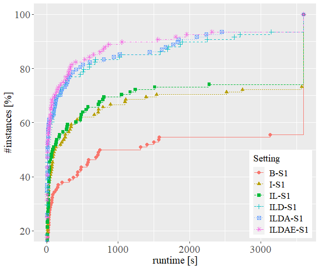
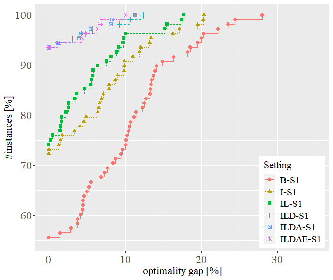
Figure 1: WMCI S1 Results.

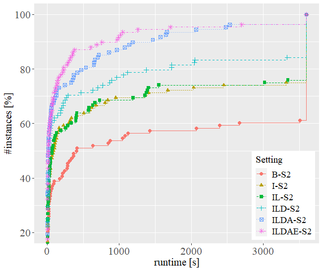
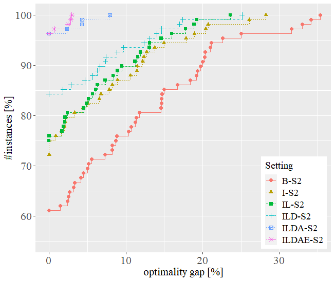
Figure 2: WMCI S2 Results.

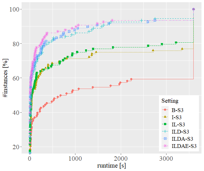
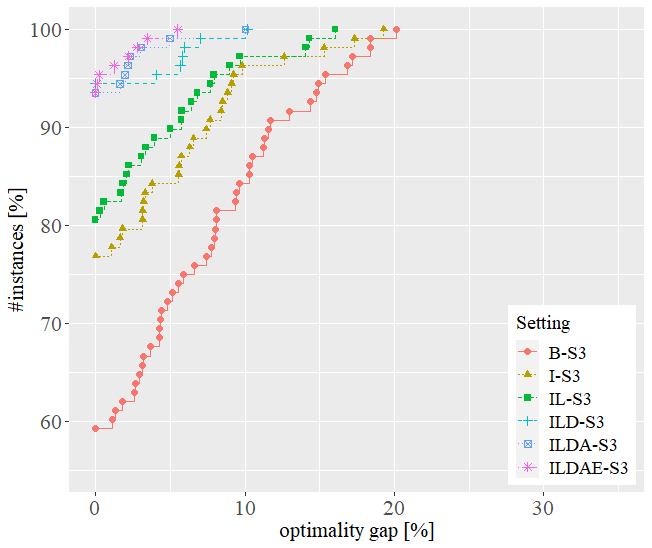
Figure 3: WMCI S3 Results.

In Figure 2, we present the results for S2. Here, while 61% of the instances are solved to optimality under the basic setting B-S2, the maximum optimality gap is 36% which is large compared to B-S1. This value remains larger until the alternative cuts are included (setting ILDA-S2) which causes a substantial decrease in running time and final gap unlike option S1. In S2, the ground set for the follower problem is defined based on a rounding scheme. Thus, the enhanced separation procedure for alternative cuts given in Section 4.4 is able to find eligible item pairs with $(x_{a_{k}}-x_{b_{k}})>0$ more easily, which explains the difference in the effect of component A under S1 and S2. After the addition of the enhanced integer separation component (E), the solution times decrease more and the maximum optimality gap is reduced to 3%. This result shows that a better search can be done when the time due to solving separation problems to optimality is saved.

The last option S3 whose results are plotted in Figure 3, yields a maximum gap of 20% under the basic setting B-S3, which is notably smaller compared to S1 and S2, although the optimal solution ratio is similar to those of the previous options. On the other hand, I-S3, IL-S3, and ILD-S3 yield better running time and final gaps than their counterparts under S1 and S2. Since alternative cuts yield a slight performance improvement compared to S2, S3 falls barely behind of S2 in the complete setting ILDAE-S3, with a maximum gap of 5%.

In Table 1, the results of the complete (ILDAE) settings of all three fractional separation options are presented in terms of running time in seconds, final gaps, root gaps, the number of branch-and-cut tree nodes, and number of SICs generated. The first three measures are also compared to those obtained with the state-of-the-art MIBLP solver, using its default setting MIX++ (Fischetti et al.,, 2017). The MIBLP formulation of WMCIG is provided in Appendix A, and the MIBLP solver is publicly available at https://msinnl.github.io/pages/bilevel.html. The numbers in the table show averages over three instances with the same parameter setting. We see that, while MIX++ is not able to solve any of the instances within the time limit of one hour and yields an average gap of $93.5\%$, this value is below $1\%$ with our settings. Even the minimum final gap obtained with MIX++, which is not reported in the table, is 54%. The difference between root gaps is also notable. The average root gap is almost 100% with MIX++ as opposed to 25% which is the average under S1, S2, and S3. When we focus only on our settings, we see that ILDAE-S2 is the best performing setting in terms of solution time, while it yields slightly larger root gaps than the others. The average tree size is considerably smaller under S3, and S2 requires the smallest number of cuts. The detailed results of all instances are given in Appendix B, Tables 3, 4, and 5.

Table 1: Results of WMCIG experiments with the complete settings (ILDAE) of each separation option and with the benchmark MIBLP solver MIX++.

	Time(sec.)				Gap(%)				rGap(%)				#Nodes			#SIC
$(n,B,k,r)$	S1	S2	S3	MIX++	S1	S2	S3	MIX++	S1	S2	S3	MIX++	S1	S2	S3	S1	S2	S3
(50,5,5,1)	0.5	0.1	2.8	TL	0.0	0.0	0.0	66.7	23.3	14.3	17.3	99.7	91.3	53.0	50.7	161.7	173.7	208.3
(50,5,5,2)	1.1	1.8	3.0	TL	0.0	0.0	0.0	73.9	18.7	15.9	17.6	100.0	230.3	216.3	190.0	219.3	249.7	331.3
(50,5,5,3)	4.0	3.2	3.0	TL	0.0	0.0	0.0	84.3	14.3	15.0	15.6	99.6	309.7	376.0	311.0	151.3	174.3	188.7
(50,5,10,1)	4.3	3.1	0.9	TL	0.0	0.0	0.0	95.4	36.2	28.9	33.8	100.0	520.7	194.7	210.0	946.0	818.3	1148.7
(50,5,10,2)	4.6	3.1	3.9	TL	0.0	0.0	0.0	88.9	28.8	26.2	29.7	100.0	1506.3	730.0	933.0	1252.3	1149.3	1705.3
(50,5,10,3)	4.7	1.9	2.5	TL	0.0	0.0	0.0	80.1	22.9	27.1	23.4	100.0	266.0	351.0	203.3	293.3	361.7	482.0
(60,6,6,1)	0.9	2.8	0.5	TL	0.0	0.0	0.0	95.9	22.7	18.7	20.0	100.0	271.3	128.3	156.7	392.7	400.7	442.3
(60,6,6,2)	5.8	32.8	12.7	TL	0.0	0.0	0.0	89.1	19.6	18.7	21.5	100.0	1029.7	1254.7	953.7	645.0	785.3	869.7
(60,6,6,3)	1.3	1.0	1.1	TL	0.0	0.0	0.0	85.1	14.8	20.4	17.6	99.4	660.7	1101.7	1058.3	305.3	410.7	441.0
(60,6,12,1)	1.6	1.8	1.9	TL	0.0	0.0	0.0	97.0	33.7	29.1	25.4	100.0	553.7	168.0	188.3	1217.0	999.3	1121.0
(60,6,12,2)	35.9	112.7	61.8	TL	0.0	0.0	0.0	94.7	28.6	30.3	30.5	100.0	6615.7	6319.3	5817.0	3449.3	4701.7	6052.3
(60,6,12,3)	4.6	8.3	4.0	TL	0.0	0.0	0.0	86.8	23.6	30.0	25.9	100.0	1128.0	2254.0	957.7	874.7	1159.0	1540.0
(70,7,7,1)	2.2	2.3	1.7	TL	0.0	0.0	0.0	98.7	23.2	20.5	22.4	100.0	746.0	242.0	315.0	895.3	821.3	1043.0
(70,7,7,2)	144.7	145.4	113.1	TL	0.0	0.0	0.0	95.9	18.4	20.9	19.3	100.0	6815.0	10818.7	8437.3	1162.7	1131.7	1273.7
(70,7,7,3)	1.1	2.8	1.6	TL	0.0	0.0	0.0	85.6	15.3	21.0	17.6	100.0	911.3	2900.3	1828.3	425.7	596.0	495.3
(70,7,14,1)	120.3	99.4	114.4	TL	0.0	0.0	0.0	97.0	35.7	32.6	33.0	100.0	5688.3	1699.0	2403.3	9265.0	7121.0	9387.0
(70,7,14,2)	820.5	1271.1	1323.3	TL	0.0	0.2	0.4	99.6	28.2	32.0	30.6	100.0	41541.7	30312.7	24504.0	12161.0	10736.3	15653.7
(70,7,14,3)	21.1	15.5	7.6	TL	0.0	0.0	0.0	88.1	24.3	30.4	27.5	100.0	3059.0	2838.3	774.7	1605.0	1752.3	1928.0
(80,8,8,1)	6.5	7.8	5.2	TL	0.0	0.0	0.0	99.4	21.8	21.3	21.9	100.0	1067.0	354.0	636.7	1521.7	1110.7	1846.3
(80,8,8,2)	189.6	152.4	154.2	TL	0.0	0.0	0.0	99.8	17.9	19.8	20.6	100.0	13628.7	20936.3	11046.7	2165.7	2428.7	2662.0
(80,8,8,3)	2.4	4.0	4.8	TL	0.0	0.0	0.0	99.9	16.1	24.9	19.8	100.0	995.7	3898.3	2453.0	470.7	692.7	667.7
(80,8,16,1)	186.4	45.9	84.7	TL	0.0	0.0	0.0	99.7	34.2	36.7	35.3	100.0	9185.3	1261.7	2677.7	12947.3	6200.7	10748.3
(80,8,16,2)	2116.9	1668.5	2939.0	TL	1.6	1.0	1.0	99.6	27.7	30.1	29.0	100.0	56039.7	28043.3	32173.7	19053.7	17227.0	27288.7
(80,8,16,3)	5.4	10.3	4.0	TL	0.0	0.0	0.0	100.0	26.2	31.3	29.8	100.0	1213.0	2961.0	694.3	1090.3	1577.0	1229.0
(90,9,9,1)	47.7	32.9	29.1	TL	0.0	0.0	0.0	97.4	19.9	21.9	21.3	100.0	4124.3	867.3	1414.3	3910.0	3220.7	3393.3
(90,9,9,2)	641.0	1110.9	1301.0	TL	0.0	0.0	0.0	95.1	17.6	18.6	18.6	100.0	42742.0	61352.0	33670.0	4936.3	4836.0	5721.0
(90,9,9,3)	5.1	6.8	2.3	TL	0.0	0.0	0.0	83.0	18.2	23.8	20.5	100.0	373.7	5118.7	914.3	651.7	908.7	901.0
(90,9,18,1)	1369.6	153.7	529.6	TL	0.0	0.0	0.0	99.3	35.3	34.8	35.3	100.0	28151.0	2666.0	5221.7	30952.3	10967.0	23276.3
(90,9,18,2)	2750.8	1555.2	1892.3	TL	2.8	0.9	1.2	99.6	25.5	30.1	30.0	100.0	50290.7	26917.0	16770.3	21869.7	16837.3	24431.7
(90,9,18,3)	24.2	45.1	19.6	TL	0.0	0.0	0.0	99.9	26.4	32.0	29.4	100.0	1668.0	9765.7	1300.7	1485.3	2788.0	2380.0
(100,10,10,1)	174.3	37.8	49.6	TL	0.0	0.0	0.0	98.7	22.6	23.5	23.2	100.0	8819.3	1452.0	2357.3	9102.3	3957.0	5558.3
(100,10,10,2)	393.1	399.6	248.8	TL	0.0	0.0	0.0	97.3	17.4	21.0	19.8	100.0	21016.7	33557.3	16961.0	4808.7	4627.7	6257.3
(100,10,10,3)	9.8	22.5	12.5	TL	0.0	0.0	0.0	94.5	18.3	26.4	21.9	100.0	909.0	10693.7	3846.3	1018.3	1462.3	1345.3
(100,10,20,1)	TL	2519.7	TL	TL	7.8	0.8	2.6	99.6	34.3	35.7	37.2	100.0	18500.7	7836.0	10143.7	54296.7	37962.0	51913.7
(100,10,20,2)	1648.9	499.2	389.8	TL	1.4	0.0	0.0	100.0	26.9	31.5	29.6	100.0	28282.7	14168.3	3974.3	12621.7	6238.0	7334.3
(100,10,20,3)	131.9	467.0	68.2	TL	0.0	0.0	0.0	99.6	29.1	35.4	31.5	99.8	8242.7	34327.0	3764.7	3279.7	5546.0	4851.0
Average	402.3	290.2	361.0	TL	0.4	0.1	0.1	93.5	24.1	25.9	25.1	100.0	10199.9	9114.8	5536.5	6155.7	4503.6	6281.0

The results are aggregated over the three instances with the same $n$, $B$, $k$, and $r$ values, and given as averages. TL indicates that the time limit of 3600 seconds is reached for all instances involved in the average.

5.2 Bipartite Inference Interdiction Game

While generating the BIIG instances, we adopt the parameter settings used in Salvagnin, (2019) for the bipartite inference problem which constitutes the lower level of BIIG. We do not include the parameter values that lead to failing to solve the problem within one hour according to their results, as we have an additional problem layer. As a result, the instances are generated as follows. The activating probability $p_{i}$ is sampled uniformly in $[0,1]$ for each $i\in N$. For the density $d$ of the graphs, i.e., the probability of having an arc between each $(i,j)$ pair, in addition to 0.07 which is the only value used in Salvagnin, (2019), two more values $\{0.1,0.15\}$ are determined, and the arcs are generated in a completely random manner. The number of items $n\in\{20,50,100\}$, the number of targets $m\in\{2n,5n,10n\}$, and number of items $B$ that the follower can choose is in $\{5,10\}$ for $n=20$, $\{10,20\}$ for $n=50$, and equal to 10 for $n=100$. The leader can interdict $k=5$ items if $n=20$ and 10 items if $n>20$. Five distinct instances are generated for each parameter setting.

The results of the experiments in terms of running time and final gaps are plotted in Figures 4, 5 and 6. Common to all three separation options, the improved cuts (I) make the largest contribution for both measures. I, IL, and ILD settings perform very similarly. In the detailed results that are not reported here, we see that the number of lifted cuts and dominance inequalities added are very small which leads to different branch-and-cut trees but not notable improvement in performance. We attribute this situation to the rareness of item pairs suitable to be used in these cuts, due to the structure of the instances, i.e., it is difficult to have that one item covers all the targets that another item covers and has a larger activation probability as described in Remark 2 and Proposition 4. Under S1 (see Figure 4), the alternative cuts cause slightly smaller solution times and maximum gap reduced from 40% to 30%. Including component H further decreases this number to 20%.

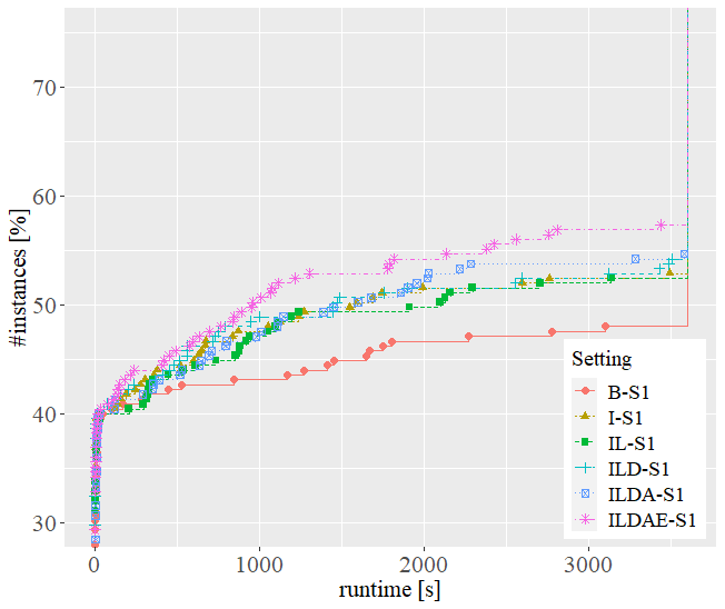
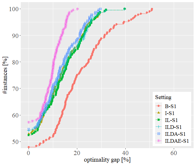
Figure 4: BIIG S1 Results.

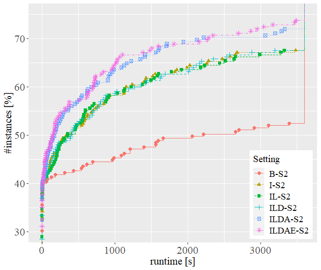
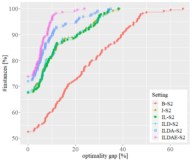
Figure 5: BIIG S2 Results.

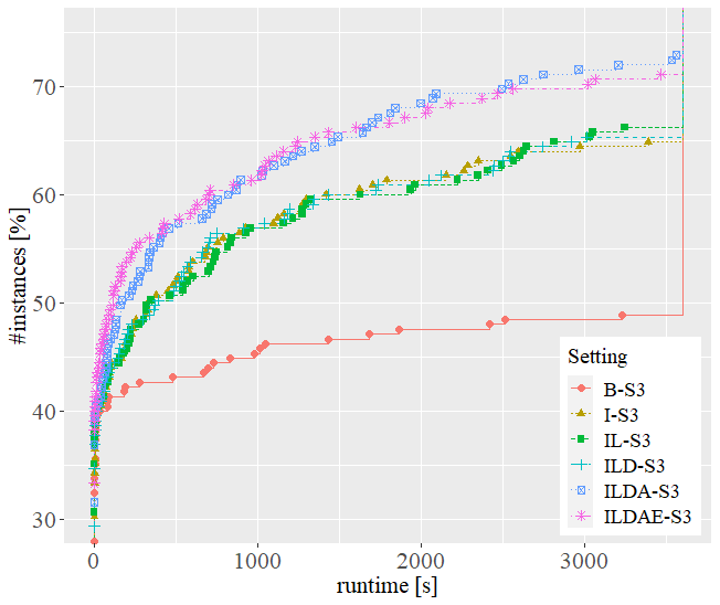
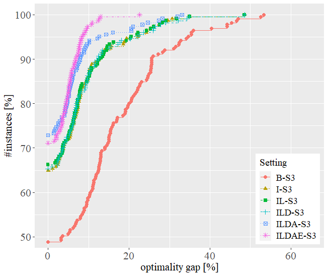
Figure 6: BIIG S3 Results.

The plots for S2 are shown in Figures 5. As is the case with WMCIG instances, B-S1 setting yields very large final optimality gaps. The increase in the number of instances solved to optimality due to the improved SICs is larger compared to S1, as can be seen from both plots. Alternative cuts have a larger contribution than they have under S1. With all the components (ILDAE-S2), the maximum optimality gap is 24% and the 74% of instances are solved to optimality within the timelimit. The performance of S3 is similar to that of S1, except the maximum gap under the basic setting which is better in the former.

Next, in Table 2 we present the average results for the ILDAE setting under all three options, with a similar structure as used in Table 1, except the MIX++ columns, since BIIG does not fit into the MIX++ setting, due to not having a compact MIBLP formulation. Each number denotes the average over five instances. In terms of running time and final gaps, while S2 and S3 perform similarly, S1 falls behind. S3 outperforms the others in terms of root gaps. As before, the tree size is smallest under S3. Since the number of instances solved to optimality is larger with this setting, it is understood that with S3 the optimal solution is reached in a smaller number of subproblems. Finally, the number of SICs generated is smaller when using S2. The detailed results for two instances from each class shown in Table 2 are provided in Appendix B, Tables 6, 7, and 8.

Table 2: Results of BIIG experiments with the complete settings (ILDAE) of each separation option.

	Time(sec.)			Gap(%)			rGap(%)			#Nodes			#SIC
$(n,m,B,k,d)$	S1	S2	S3	S1	S2	S3	S1	S2	S3	S1	S2	S3	S1	S2	S3
(20,40,5,5,0.07)	0.8	0.1	0.1	0.0	0.0	0.0	40.8	25.8	25.0	151.6	63.4	71.0	185.0	208.0	253.4
(20,40,5,5,0.10)	0.1	0.1	0.2	0.0	0.0	0.0	38.2	22.9	23.1	92.8	49.8	42.8	142.0	151.8	177.2
(20,40,5,5,0.15)	1.2	0.3	0.5	0.0	0.0	0.0	37.7	27.0	24.1	139.2	56.6	50.0	194.4	202.8	252.2
(20,40,10,5,0.07)	0.6	0.3	0.1	0.0	0.0	0.0	26.4	25.0	10.2	101.2	38.2	12.8	108.0	135.4	77.8
(20,40,10,5,0.10)	2.1	0.1	0.4	0.0	0.0	0.0	27.4	26.2	16.5	174.0	63.6	28.4	182.2	194.0	135.4
(20,40,10,5,0.15)	1.2	0.1	0.2	0.0	0.0	0.0	24.2	25.5	21.4	302.2	74.4	46.8	378.0	252.0	252.8
(20,100,5,5,0.07)	1.8	0.2	1.0	0.0	0.0	0.0	37.5	23.0	23.0	93.4	32.8	43.8	152.6	144.2	185.2
(20,100,5,5,0.10)	2.0	1.7	0.2	0.0	0.0	0.0	39.9	27.7	25.0	144.0	57.6	63.2	192.6	221.2	253.8
(20,100,5,5,0.15)	3.2	0.6	0.2	0.0	0.0	0.0	34.8	24.4	25.8	119.4	39.4	45.8	202.0	203.8	275.8
(20,100,10,5,0.07)	3.3	3.1	1.5	0.0	0.0	0.0	27.3	26.6	16.8	278.0	78.0	25.6	289.8	283.2	145.4
(20,100,10,5,0.10)	10.2	1.7	0.7	0.0	0.0	0.0	28.1	27.3	20.7	620.4	168.0	93.6	667.0	589.4	500.0
(20,100,10,5,0.15)	8.8	0.7	0.3	0.0	0.0	0.0	28.6	29.4	24.3	497.8	140.2	71.0	582.2	471.4	432.4
(20,200,5,5,0.07)	0.2	0.2	0.2	0.0	0.0	0.0	38.6	23.2	23.2	116.4	36.6	45.0	167.4	143.0	172.4
(20,200,5,5,0.10)	2.4	1.0	0.2	0.0	0.0	0.0	39.8	24.1	22.9	122.2	57.4	61.6	200.6	221.8	272.4
(20,200,5,5,0.15)	0.6	0.4	1.1	0.0	0.0	0.0	40.4	27.6	27.9	174.4	55.6	67.6	287.0	279.6	340.4
(20,200,10,5,0.07)	1.0	0.2	0.4	0.0	0.0	0.0	25.8	24.2	15.5	273.4	67.8	32.8	295.2	252.0	179.0
(20,200,10,5,0.10)	6.0	1.8	0.8	0.0	0.0	0.0	29.6	29.0	20.8	642.6	169.4	116.0	852.6	615.2	586.4
(20,200,10,5,0.15)	3.6	3.1	2.0	0.0	0.0	0.0	29.0	28.6	27.1	1242.4	361.2	206.6	1509.4	1062.8	1127.6
(50,100,10,10,0.07)	742.6	71.1	54.5	0.0	0.0	0.0	39.8	33.6	33.7	13243.2	1066.4	1100.6	19297.2	5950.6	7381.0
(50,100,10,10,0.10)	495.0	70.3	44.7	0.0	0.0	0.0	40.4	35.5	33.4	10887.0	1135.0	1079.6	19737.0	6451.4	7945.4
(50,100,10,10,0.15)	1251.0	291.8	291.5	0.0	0.0	0.0	38.1	36.9	36.2	17118.2	3012.8	2671.4	30409.2	13284.6	17265.2
(50,100,20,10,0.07)	3094.1	167.3	74.0	3.7	0.0	0.0	25.4	27.4	24.8	30110.6	2761.2	980.4	44845.6	14129.6	7556.6
(50,100,20,10,0.10)	TL	3426.5	3493.3	12.6	2.2	3.0	29.1	27.7	28.0	17823.4	13535.0	5847.4	43050.2	60934.2	50894.8
(50,100,20,10,0.15)	TL	3176.4	3129.2	11.9	6.2	5.1	28.2	29.2	28.2	13805.8	10767.4	5591.4	36628.6	46254.8	48118.4
(50,250,10,10,0.07)	1254.7	214.3	195.4	1.1	0.0	0.0	38.9	34.1	34.3	17169.8	1778.8	1816.0	33312.2	11623.2	14706.6
(50,250,10,10,0.10)	1476.3	344.1	444.3	0.7	0.0	0.0	38.6	35.8	36.0	20454.2	3021.6	2607.0	38334.8	17439.0	22967.8
(50,250,10,10,0.15)	2481.5	596.7	571.5	1.0	0.0	0.0	40.4	38.8	38.2	27197.2	4770.8	3521.4	52997.4	25344.8	31984.4
(50,250,20,10,0.07)	TL	2832.2	1663.8	10.5	3.0	1.5	29.3	28.7	27.9	24945.8	7078.4	3236.4	54231.0	44474.8	31120.0
(50,250,20,10,0.10)	TL	TL	TL	14.6	7.1	6.2	31.1	29.4	29.9	23904.0	7229.2	4432.6	55816.2	53267.2	53847.2
(50,250,20,10,0.15)	TL	TL	TL	13.2	7.2	7.8	29.4	29.3	28.3	17563.8	10147.0	4457.4	52104.4	54222.2	52020.0
(50,500,10,10,0.07)	1394.1	239.9	244.2	1.2	0.0	0.0	41.2	36.3	34.7	18172.4	1909.6	2095.6	36983.0	12595.4	17501.2
(50,500,10,10,0.10)	2286.9	1470.1	1452.6	4.8	0.7	0.7	40.2	36.8	37.4	18616.2	4365.2	3773.4	48691.2	30415.6	38090.8
(50,500,10,10,0.15)	2457.4	616.0	1276.7	3.0	0.0	0.0	38.9	38.9	38.0	19249.4	4608.0	4069.2	46038.0	26010.8	37769.0
(50,500,20,10,0.07)	TL	2470.5	2577.9	11.9	3.1	3.6	28.7	28.3	27.6	21951.0	5431.0	3118.6	51392.4	41838.0	37029.0
(50,500,20,10,0.10)	TL	TL	TL	16.6	8.8	7.9	30.5	30.1	29.7	16875.2	6230.8	4408.8	47643.2	50604.0	57941.8
(50,500,20,10,0.15)	TL	TL	TL	14.9	11.7	12.2	30.1	29.8	30.1	14172.6	6352.2	3858.2	48670.0	41906.6	46339.2
(100,200,10,10,0.07)	3095.6	906.7	1607.6	4.8	0.0	0.7	31.3	30.2	30.5	21226.4	6033.8	6315.4	58458.4	24640.2	38734.6
(100,200,10,10,0.10)	3431.6	1880.5	1824.4	6.7	1.1	1.2	29.7	31.5	31.5	20834.4	8998.0	7423.8	53874.6	31265.0	43205.0
(100,200,10,10,0.15)	TL	2906.7	TL	9.7	4.7	3.6	28.4	32.5	31.4	10258.2	8524.6	6958.6	36347.2	24304.2	49364.6
(100,500,10,10,0.07)	TL	2218.3	2543.1	8.2	1.1	1.7	31.9	31.6	31.5	15180.4	6239.4	5944.8	63577.6	41637.6	54433.2
(100,500,10,10,0.10)	TL	3349.6	TL	9.6	3.8	4.3	30.3	32.3	31.8	14783.8	7862.6	6286.6	60239.8	49257.4	67210.4
(100,500,10,10,0.15)	TL	3577.4	TL	12.7	9.5	6.2	29.0	34.2	32.4	6514.2	6679.8	4145.4	31428.2	26154.8	46963.4
(100,1000,10,10,0.07)	3568.3	2936.3	3315.2	7.0	3.0	3.6	31.4	33.3	31.9	15108.0	4373.4	5407.8	68691.6	42208.6	63986.0
(100,1000,10,10,0.10)	TL	3052.2	3484.5	8.6	2.7	4.2	31.4	34.6	33.5	13707.4	6304.0	5070.0	66499.8	48547.6	62304.0
(100,1000,10,10,0.15)	TL	TL	TL	12.5	9.6	8.3	29.7	36.3	33.3	6278.2	6410.6	3571.6	34473.2	33760.2	43062.8
Average	1721.7	1218.5	1268.9	4.5	1.9	1.8	33.0	30.0	27.9	10498.6	3516.4	2464.8	27563.6	19647.9	23452.5

The results are aggregated over the five instances with the same $n$, $m$, $B$, $k$, and $d$ values, and given as averages. TL indicates that the time limit of 3600 seconds is reached for all instances involved in the average.

6 Conclusion

In this paper, we have presented an exact method to solve interdiction games with a submodular and non-decreasing objective function. Such problems have many real world applications as described in Section 1.1. We introduce submodular interdiction cuts (SIC) by exploiting the special properties of submodular set functions. We also develop improved and lifted variants of these SIC. The branch-and-cut framework which we design based on SICs involves several other components such as dominance inequalities, greedy algorithms for separation of fractional solutions and an enhanced separation procedure for integer solutions. We also investigate the impact of using maximal sets while building SICs instead of non-maximal ones, and utilize the obtained information to design better separation schemes.

To assess the performance of our solution algorithm and its individual components, we conduct a computational study on the weighted maximal covering interdiction game and the bipartite inference interdiction game. The results show that the components of our framework provide significant improvements with respect to the basic version. Moreover, our method vastly outperforms a state-of-the-art general purpose mixed-integer bilevel linear programming (MIBLP) solver for the weighted maximal covering interdiction game (for which a MIBLP formulation is possible).

Regarding further work, a natural extension of interdiction games is the fortification problem where a third problem layer includes the interdiction game as a constraint. There are several studies addressing defender-attacker-defender games such as Cappanera and Scaparra, (2011), Lozano and Smith, 2017a , Lozano et al., (2017), and Zheng and Albert, (2018). It could be interesting to study such games with submodular objective function. Another possible future research direction could be developing methods for the solution of stochastic or robust submodular interdiction games. Finally, one could also focus on concrete submodular interdiction games and try to extend our general-purpose framework with problem-specific components.

Appendix A The MIBLP Formulation of WMCIG

Let binary leader variables $x_{i}$, $i\in N$ indicate the interdiction decisions of the leader. Let binary follower variables $y_{i}$, $i\in N$ take the value one if and only if facility $i\in N$ is open in a solution. Let binary follower variables $z_{j}$, $j\in J$ take the value one if and only if customer $j$ is covered in a solution. The following formulation is used while solving WMCIG instances by the MIBLP solver MIX++.

$$\min_{x\in X}\,\max_{y,z} \,\sum_{j\in J}p_{j}z_{j}$$

s.t. $$\,\sum_{i\in N}y_{i}\leq B$$

$$z_{j}\leq\sum_{i:j\in J(i)}y_{i} \forall j \in J$$

$$y_{i}\leq 1-x_{i} \forall i \in N$$

$$y_{i}\in\{0,1\} \forall i \in N$$

$$z_{j}\in\{0,1\} \forall j \in J$$

where $X=\{x\in\{0,1\}^{|N|}:\sum_{i\in N}x_{i}\leq k\}$.

Appendix B Detailed Results

Table 3: Detailed WMCIG results under separation option S2: basic and complete setting comparison.

	B-S2							ILDAE-S2
$(n,B,p,r,ID)$	t(s.)	UB	LB	Gap(%)	rGap(%)	#Nodes	#SIC	t(s.)	UB	LB	Gap(%)	rGap(%)	#Nodes	#SIC
(50,5,5,1,1)	1	882	882.0	0.0	30.3	118	154	0	882	882.0	0.0	12.2	11	80
(50,5,5,1,2)	1	883	883.0	0.0	31.4	258	240	0	883	883.0	0.0	13.1	78	213
(50,5,5,1,3)	3	1003	1003.0	0.0	27.2	224	186	0	1003	1003.0	0.0	17.5	70	228
(50,5,5,2,1)	12	1852	1852.0	0.0	24.1	658	178	1	1852	1852.0	0.0	16.5	58	200
(50,5,5,2,2)	3	1835	1835.0	0.0	25.9	511	183	1	1835	1835.0	0.0	14.6	181	278
(50,5,5,2,3)	12	2031	2031.0	0.0	28.9	730	184	4	2031	2031.0	0.0	16.6	410	271
(50,5,5,3,1)	2	2442	2442.0	0.0	27.6	1085	233	1	2442	2442.0	0.0	15.2	306	153
(50,5,5,3,2)	9	2171	2171.0	0.0	25.5	1593	164	8	2171	2171.0	0.0	14.1	435	170
(50,5,5,3,3)	5	2383	2383.0	0.0	26.4	953	125	0	2383	2383.0	0.0	15.8	387	200
(50,5,10,1,1)	8	828	827.9	0.0	41.7	2006	1432	0	828	828.0	0.0	25.5	158	594
(50,5,10,1,2)	2	933	933.0	0.0	45.4	1777	1069	4	933	933.0	0.0	31.2	93	457
(50,5,10,1,3)	8	720	720.0	0.0	43.8	3861	2168	5	720	720.0	0.0	29.9	333	1404
(50,5,10,2,1)	5	1747	1746.9	0.0	40.0	4333	1247	1	1747	1747.0	0.0	26.4	396	960
(50,5,10,2,2)	8	1587	1586.8	0.0	39.8	7927	1373	3	1587	1587.0	0.0	25.9	827	1239
(50,5,10,2,3)	19	1634	1634.0	0.0	36.6	7230	1174	5	1634	1633.9	0.0	26.5	967	1249
(50,5,10,3,1)	30	2353	2353.0	0.0	37.7	6482	942	3	2353	2353.0	0.0	27.0	243	270
(50,5,10,3,2)	10	2287	2286.9	0.0	40.8	5371	911	1	2287	2287.0	0.0	28.6	257	285
(50,5,10,3,3)	21	2024	2023.8	0.0	40.9	13688	1004	3	2024	2024.0	0.0	25.8	553	530
(60,6,6,1,1)	1	1115	1115.0	0.0	30.0	571	513	8	1115	1115.0	0.0	19.0	83	262
(60,6,6,1,2)	12	1391	1391.0	0.0	31.6	1108	529	0	1391	1391.0	0.0	17.8	99	383
(60,6,6,1,3)	1	1326	1326.0	0.0	31.3	1064	506	1	1326	1326.0	0.0	19.3	203	557
(60,6,6,2,1)	71	2625	2625.0	0.0	26.8	4338	429	66	2625	2625.0	0.0	18.6	1972	791
(60,6,6,2,2)	24	2463	2463.0	0.0	26.3	3006	507	7	2463	2462.9	0.0	18.2	873	741
(60,6,6,2,3)	62	2238	2238.0	0.0	32.0	1650	498	25	2238	2238.0	0.0	19.4	919	824
(60,6,6,3,1)	3	2994	2994.0	0.0	29.5	6562	560	1	2994	2994.0	0.0	22.0	593	372
(60,6,6,3,2)	4	2813	2812.8	0.0	32.0	3650	482	1	2813	2812.9	0.0	19.4	949	335
(60,6,6,3,3)	8	2944	2944.0	0.0	29.0	8824	544	1	2944	2943.8	0.0	19.7	1763	525
(60,6,12,1,1)	11	1031	1031.0	0.0	38.7	4281	2638	1	1031	1031.0	0.0	27.2	116	781
(60,6,12,1,2)	37	935	935.0	0.0	42.9	12834	5639	3	935	935.0	0.0	31.1	341	1840
(60,6,12,1,3)	7	995	995.0	0.0	43.0	2073	2060	2	995	995.0	0.0	29.2	47	377
(60,6,12,2,1)	334	2385	2384.8	0.0	34.8	65219	5285	186	2385	2384.8	0.0	29.0	3819	4670
(60,6,12,2,2)	364	2029	2028.8	0.0	36.9	102142	6493	140	2029	2028.8	0.0	31.9	13480	6947
(60,6,12,2,3)	95	2252	2252.0	0.0	36.7	33502	5148	12	2252	2251.9	0.0	30.1	1659	2488
(60,6,12,3,1)	214	2493	2492.8	0.0	46.9	64054	4787	1	2493	2493.0	0.0	31.9	304	467
(60,6,12,3,2)	307	2673	2673.0	0.0	40.8	73903	5019	14	2673	2672.9	0.0	29.1	1989	1173
(60,6,12,3,3)	283	2547	2547.0	0.0	47.8	116603	4638	10	2547	2546.8	0.0	29.0	4469	1837

Table 4: Detailed WMCIG results under separation option S2: basic and complete setting comparison (continued).

	B-S2							ILDAE-S2
$(n,B,p,r,ID)$	t(s.)	UB	LB	Gap(%)	rGap(%)	#Nodes	#SIC	t(s.)	UB	LB	Gap(%)	rGap(%)	#Nodes	#SIC
(70,7,7,1,1)	7	1441	1441.0	0.0	31.7	4292	1952	5	1441	1441.0	0.0	19.4	278	1017
(70,7,7,1,2)	6	1427	1427.0	0.0	31.0	3745	1645	2	1427	1427.0	0.0	22.4	243	859
(70,7,7,1,3)	6	1567	1567.0	0.0	30.4	2639	1910	1	1567	1567.0	0.0	19.7	205	588
(70,7,7,2,1)	243	2785	2785.0	0.0	27.6	8306	1738	76	2785	2785.0	0.0	20.2	1200	1104
(70,7,7,2,2)	366	3225	3224.7	0.0	26.2	22000	1262	131	3225	3224.7	0.0	20.2	9623	1324
(70,7,7,2,3)	847	3122	3121.8	0.0	29.1	55435	796	229	3122	3121.8	0.0	22.2	21633	967
(70,7,7,3,1)	45	3196	3195.7	0.0	28.3	42733	1789	5	3196	3195.7	0.0	22.5	6253	611
(70,7,7,3,2)	9	3293	3292.8	0.0	33.4	11951	1558	2	3293	3292.7	0.0	20.3	1391	762
(70,7,7,3,3)	42	3318	3317.7	0.0	34.5	31078	1285	2	3318	3318.0	0.0	20.2	1057	415
(70,7,14,1,1)	86	1288	1287.9	0.0	40.4	13126	8263	3	1288	1288.0	0.0	31.3	321	1200
(70,7,14,1,2)	TL	1400	1355.5	3.2	45.0	179438	50192	289	1400	1399.9	0.0	33.5	4358	18345
(70,7,14,1,3)	206	1331	1330.9	0.0	42.6	18283	11931	6	1331	1331.0	0.0	33.2	418	1818
(70,7,14,2,1)	TL	2940	2776.2	5.6	39.5	179608	20917	159	2940	2939.7	0.0	33.6	11097	7885
(70,7,14,2,2)	873	2647	2646.7	0.0	38.5	48718	6268	55	2647	2647.0	0.0	30.0	596	1138
(70,7,14,2,3)	TL	3001	2847.4	5.1	37.3	306010	22123	TL	3001	2982.2	0.6	32.4	79245	23186
(70,7,14,3,1)	TL	3409	3317.9	2.7	40.5	221008	13647	13	3409	3409.0	0.0	31.3	4102	1830
(70,7,14,3,2)	2396	3065	3064.7	0.0	40.0	200286	9799	23	3065	3064.8	0.0	31.4	2285	2185
(70,7,14,3,3)	2673	3054	3053.7	0.0	47.8	181042	11194	11	3054	3054.0	0.0	28.5	2128	1242
(80,8,8,1,1)	18	1852	1851.9	0.0	28.6	6562	3300	3	1852	1852.0	0.0	19.4	240	802
(80,8,8,1,2)	16	1896	1896.0	0.0	32.4	5670	3493	3	1896	1896.0	0.0	21.1	325	835
(80,8,8,1,3)	22	1915	1915.0	0.0	30.6	7969	3345	18	1915	1915.0	0.0	23.5	497	1695
(80,8,8,2,1)	1424	3603	3602.6	0.0	29.0	56405	4443	113	3603	3602.6	0.0	20.5	11148	2887
(80,8,8,2,2)	1078	3340	3339.7	0.0	28.4	141737	3041	272	3340	3339.7	0.0	20.0	39300	2192
(80,8,8,2,3)	1043	3312	3311.7	0.0	27.6	110767	2756	73	3312	3311.7	0.0	18.9	12361	2207
(80,8,8,3,1)	171	3860	3859.6	0.0	34.7	60099	3841	1	3860	3860.0	0.0	22.6	1526	556
(80,8,8,3,2)	635	3818	3818.0	0.0	40.6	190382	6860	7	3818	3818.0	0.0	25.4	7503	807
(80,8,8,3,3)	282	4501	4500.6	0.0	40.2	121391	3197	3	4501	4500.6	0.0	26.6	2666	715
(80,8,16,1,1)	TL	1537	1411.0	8.2	45.1	80358	64277	79	1537	1536.9	0.0	36.5	2040	8442
(80,8,16,1,2)	TL	1607	1464.8	8.8	44.4	84609	62889	30	1586	1585.8	0.0	36.7	876	5354
(80,8,16,1,3)	TL	1569	1498.4	4.5	45.7	88200	52448	28	1569	1569.0	0.0	36.9	869	4806
(80,8,16,2,1)	TL	3547	3179.4	10.4	38.9	78427	18223	357	3534	3533.7	0.0	30.5	11053	11962
(80,8,16,2,2)	TL	3510	2999.2	14.6	38.0	54756	14970	TL	3494	3390.6	3.0	31.1	32400	23595
(80,8,16,2,3)	TL	3243	2768.1	14.6	38.4	52184	13611	1048	3196	3195.7	0.0	28.8	40677	16124
(80,8,16,3,1)	TL	3685	3251.0	11.8	50.3	150519	17079	15	3618	3617.7	0.0	30.9	4872	1900
(80,8,16,3,2)	TL	3382	3296.0	2.5	47.5	135481	14476	4	3382	3382.0	0.0	28.7	1185	1045
(80,8,16,3,3)	TL	3305	3017.7	8.7	53.1	141120	14903	12	3296	3295.7	0.0	34.3	2826	1786

Table 5: Detailed WMCIG results under separation option S2: basic and complete setting comparison (continued).

	B-S2							ILDAE-S2
$(n,B,p,r,ID)$	t(s.)	UB	LB	Gap(%)	rGap(%)	#Nodes	#SIC	t(s.)	UB	LB	Gap(%)	rGap(%)	#Nodes	#SIC
(90,9,9,1,1)	22	2343	2343.0	0.0	30.6	3950	4978	7	2343	2343.0	0.0	20.4	140	983
(90,9,9,1,2)	409	1860	1859.8	0.0	29.4	49727	15633	50	1860	1859.9	0.0	23.0	1442	4343
(90,9,9,1,3)	274	2447	2446.8	0.0	29.4	29199	11829	42	2447	2446.8	0.0	22.2	1020	4336
(90,9,9,2,1)	TL	4579	4427.7	3.3	29.3	119802	8017	604	4579	4578.6	0.0	20.7	34771	4065
(90,9,9,2,2)	TL	3909	3082.0	21.2	25.7	70	145	1710	3887	3886.6	0.0	16.8	59925	4468
(90,9,9,2,3)	TL	4273	3485.6	18.4	27.4	1110	625	1019	4190	4189.6	0.0	18.4	89360	5975
(90,9,9,3,1)	TL	4574	4465.5	2.4	38.7	374194	9400	6	4574	4573.6	0.0	24.1	6241	886
(90,9,9,3,2)	TL	5147	5072.1	1.5	41.8	362315	13868	4	5147	5146.6	0.0	23.6	2473	831
(90,9,9,3,3)	3511	4137	4136.6	0.0	38.0	373095	8215	10	4137	4136.7	0.0	23.7	6642	1009
(90,9,18,1,1)	TL	1966	1671.6	15.0	42.3	45800	62635	143	1949	1948.9	0.0	34.8	2225	11965
(90,9,18,1,2)	TL	1875	1661.8	11.4	42.3	53600	58722	225	1867	1866.8	0.0	34.8	3675	12381
(90,9,18,1,3)	TL	1709	1517.6	11.2	41.6	49606	49914	93	1707	1707.0	0.0	34.9	2098	8555
(90,9,18,2,1)	TL	4111	3180.5	22.6	38.7	5200	3791	379	3861	3860.7	0.0	31.1	7910	8876
(90,9,18,2,2)	TL	4372	2989.9	31.6	39.0	900	1284	TL	4056	3941.5	2.8	28.3	43714	28317
(90,9,18,2,3)	TL	3726	2980.1	20.0	36.7	6900	6812	686	3630	3629.6	0.0	30.8	29127	13319
(90,9,18,3,1)	TL	4389	3289.9	25.0	57.0	79511	31949	35	4266	4265.6	0.0	30.5	8296	3647
(90,9,18,3,2)	TL	4647	3728.5	19.8	63.3	86129	23560	93	4557	4556.6	0.0	34.9	18263	3319
(90,9,18,3,3)	TL	4035	3255.0	19.3	57.3	68008	24866	8	3969	3968.6	0.0	30.6	2738	1398
(100,10,10,1,1)	2071	2605	2604.7	0.0	31.1	103857	28889	66	2605	2604.8	0.0	22.0	2471	6374
(100,10,10,1,2)	1123	2486	2485.8	0.0	32.7	46843	26071	32	2486	2485.9	0.0	26.8	1565	3842
(100,10,10,1,3)	403	2424	2423.8	0.0	31.2	32035	12850	15	2424	2423.9	0.0	21.8	320	1655
(100,10,10,2,1)	TL	4163	3551.4	14.7	27.5	3199	2043	758	4091	4090.6	0.0	21	28611	5282
(100,10,10,2,2)	TL	4328	4148.5	4.1	25.8	67344	11120	116	4317	4316.6	0.0	20.5	5268	2666
(100,10,10,2,3)	TL	4271	4057.2	5.0	30.5	115011	10229	324	4271	4270.6	0.0	21.6	66793	5935
(100,10,10,3,1)	TL	4871	4350.3	10.7	42.4	181107	24528	21	4851	4850.5	0.0	25.9	12279	1562
(100,10,10,3,2)	TL	5264	4831.7	8.2	43.1	137616	20799	23	5264	5264.0	0.0	26.6	4581	1410
(100,10,10,3,3)	TL	4430	4106.3	7.3	40.6	264138	14489	24	4430	4429.6	0.0	26.7	15221	1415
(100,10,20,1,1)	TL	2274	1812.1	20.3	43.9	33100	62332	TL	2243	2187.4	2.5	36.0	9237	49097
(100,10,20,1,2)	TL	2575	2080.0	19.2	41.3	32700	51822	1258	2538	2537.8	0.0	35.5	5245	27756
(100,10,20,1,3)	TL	2101	1659.7	21.0	42.0	30204	55337	2701	2074	2073.8	0.0	35.7	9026	37033
(100,10,20,2,1)	TL	4378	3735.5	14.7	42.2	55400	24859	311	4278	4277.6	0.0	31.9	9821	5672
(100,10,20,2,2)	TL	4523	3606.2	20.3	39.8	2881	3736	215	4279	4278.6	0.0	31.1	6095	4390
(100,10,20,2,3)	TL	4681	3897.3	16.7	42.8	34217	14905	972	4521	4520.6	0.0	31.4	26589	8652
(100,10,20,3,1)	TL	5022	3364.9	33.0	67.6	74907	28993	349	4911	4910.5	0.0	35.2	38637	5308
(100,10,20,3,2)	TL	4917	3239.4	34.1	63.1	68400	30693	63	4523	4523.0	0.0	34.9	16533	3055
(100,10,20,3,3)	TL	4825	3120.3	35.3	64.5	66800	26868	989	4609	4608.6	0.0	36.0	47811	8275
Average	1606.5	2778.4	2569.9	5.4	37.5	62216.6	12235.8	290.3	2753.7	2750.9	0.1	25.9	9114.8	4503.6

Table 6: Detailed BIIG results under separation option S2: basic and complete setting comparison.

	B-S2							ILDAE-S2
$(n,m,B,p,d,ID)$	t(s.)	UB	LB	Gap(%)	rGap(%)	#Nodes	#SIC	t(s.)	UB	LB	Gap(%)	rGap(%)	#Nodes	#SIC
(20,40,5,5,0.07,1)	0	7	7.0	0.0	43.0	156	173	0	7	7.0	0.0	28.4	92	305
(20,40,5,5,0.07,2)	1	9	9.0	0.0	43.9	110	146	0	9	9.0	0.0	30.4	61	226
(20,40,5,5,0.10,1)	0	9.8	9.8	0.0	43.5	121	120	0	9.8	9.8	0.0	22.8	79	207
(20,40,5,5,0.10,2)	0	8.8	8.8	0.0	41.7	35	53	0	8.8	8.8	0.0	23.0	17	62
(20,40,5,5,0.15,1)	0	12.1	12.1	0.0	33.1	48	57	0	12.1	12.1	0.0	22.1	31	104
(20,40,5,5,0.15,2)	1	19.5	19.5	0.0	46.0	255	220	1	19.5	19.5	0.0	31.2	125	386
(20,40,10,5,0.07,1)	0	11	11.0	0.0	31.3	48	101	0	11	11.0	0.0	22.8	37	125
(20,40,10,5,0.07,2)	0	8.7	8.7	0.0	26.5	40	81	0	8.7	8.7	0.0	21.0	26	111
(20,40,10,5,0.10,1)	0	12.6	12.6	0.0	32.5	57	92	0	12.6	12.6	0.0	24.2	27	78
(20,40,10,5,0.10,2)	0	16.1	16.1	0.0	38.8	107	184	0	16.1	16.1	0.0	27.0	78	216
(20,40,10,5,0.15,1)	0	15.6	15.6	0.0	32.6	78	147	0	15.6	15.6	0.0	21.8	46	139
(20,40,10,5,0.15,2)	1	21.1	21.1	0.0	41.3	335	694	0	21.1	21.1	0.0	29.0	60	265
(20,100,5,5,0.07,1)	0	18	18.0	0.0	40.9	106	147	0	18	18.0	0.0	29.8	57	212
(20,100,5,5,0.07,2)	1	17.1	17.1	0.0	33.6	53	89	0	17.1	17.1	0.0	18.1	28	108
(20,100,5,5,0.10,1)	1	29.1	29.1	0.0	41.2	92	127	4	29.1	29.1	0.0	25.8	54	213
(20,100,5,5,0.10,2)	1	30.7	30.7	0.0	48.1	198	245	2	30.7	30.7	0.0	30.4	94	387
(20,100,5,5,0.15,1)	0	43.2	43.2	0.0	40.4	264	183	0	43.2	43.2	0.0	21.3	52	319
(20,100,5,5,0.15,2)	0	38.8	38.8	0.0	46.6	115	156	0	38.8	38.8	0.0	29.1	40	173
(20,100,10,5,0.07,1)	5	22.2	22.2	0.0	29.1	27	65	0	22.2	22.2	0.0	22.5	22	72
(20,100,10,5,0.07,2)	2	25.1	25.1	0.0	34.4	191	339	15	25.1	25.1	0.0	29.2	106	394
(20,100,10,5,0.10,1)	6	45.6	45.6	0.0	42.9	1187	1622	3	45.6	45.6	0.0	29.0	397	1345
(20,100,10,5,0.10,2)	7	42.3	42.3	0.0	39.9	292	529	0	42.3	42.3	0.0	27.2	129	400
(20,100,10,5,0.15,1)	0	54.1	54.1	0.0	45.1	208	393	0	54.1	54.1	0.0	32.7	78	224
(20,100,10,5,0.15,2)	3	49.6	49.6	0.0	42.2	392	763	0	49.6	49.6	0.0	29.6	116	377
(20,200,5,5,0.07,1)	3	34.1	34.1	0.0	37.6	104	134	0	34.1	34.1	0.0	24.7	69	206
(20,200,5,5,0.07,2)	0	34.4	34.4	0.0	41.9	54	80	0	34.4	34.4	0.0	23.6	23	92
(20,200,5,5,0.10,1)	1	50.1	50.1	0.0	35.8	114	130	1	50.1	50.1	0.0	25.2	30	203
(20,200,5,5,0.10,2)	0	63.8	63.8	0.0	48.0	202	241	3	63.8	63.8	0.0	31.9	156	507
(20,200,5,5,0.15,1)	4	68.2	68.2	0.0	40.5	128	162	0	68.2	68.2	0.0	26.3	31	171
(20,200,5,5,0.15,2)	0	90.7	90.7	0.0	47.4	173	203	0	90.7	90.7	0.0	27.2	49	311
(20,200,10,5,0.07,1)	1	40.3	40.3	0.0	29.7	103	201	0	40.3	40.3	0.0	23.6	60	235
(20,200,10,5,0.07,2)	0	48.4	48.4	0.0	32.8	121	219	0	48.4	48.4	0.0	29.2	82	278
(20,200,10,5,0.10,1)	3	80.2	80.2	0.0	45.3	978	1462	5	80.2	80.2	0.0	33.0	264	912
(20,200,10,5,0.10,2)	4	89.9	89.9	0.0	43.2	736	1215	1	89.9	89.9	0.0	30.5	201	771
(20,200,10,5,0.15,1)	8	106.7	106.7	0.0	40.5	1025	1670	2	106.7	106.7	0.0	26.6	182	820
(20,200,10,5,0.15,2)	1	101.9	101.9	0.0	44.0	369	606	1	101.9	101.9	0.0	27.4	134	401

Table 7: Detailed BIIG results under separation option S2: basic and complete setting comparison (continued).

	B-S2							ILDAE-S2
$(n,m,B,p,d,ID)$	t(s.)	UB	LB	Gap(%)	rGap(%)	#Nodes	#SIC	t(s.)	UB	LB	Gap(%)	rGap(%)	#Nodes	#SIC
(50,100,10,10,0.07,1)	129	34.9	34.9	0.0	44.8	5011	10904	17	34.9	34.9	0.0	29.9	518	2742
(50,100,10,10,0.07,2)	1399	39.7	39.7	0.0	50.4	30357	39996	100	39.7	39.7	0.0	34.7	1711	10919
(50,100,10,10,0.10,1)	544	49.8	49.8	0.0	53.7	15896	27497	43	49.8	49.8	0.0	32.1	989	5323
(50,100,10,10,0.10,2)	77	42.7	42.7	0.0	46.4	3854	9208	11	42.7	42.7	0.0	34.6	380	2187
(50,100,10,10,0.15,1)	2215	66.6	66.6	0.0	59.6	52408	52320	221	66.6	66.6	0.0	38.4	2481	11722
(50,100,10,10,0.15,2)	2705	64	64.0	0.0	51.7	72302	53658	182	64	64.0	0.0	36.2	2145	12375
(50,100,20,10,0.07,1)	TL	56.9	49.8	12.4	42.4	10400	50273	119	55.5	55.5	0.0	27.5	2421	12942
(50,100,20,10,0.07,2)	TL	44.7	41.2	7.9	41.1	14311	60255	144	44.4	44.4	0.0	25.8	3021	14765
(50,100,20,10,0.10,1)	TL	75.7	55.6	26.5	54.0	9680	51406	TL	74.5	70.5	5.3	27.1	12537	64302
(50,100,20,10,0.10,2)	TL	75.3	57.5	23.7	50.6	10018	49087	TL	73.9	72.0	2.5	25.6	16016	59568
(50,100,20,10,0.15,1)	TL	86.4	54.9	36.4	60.8	5604	25833	TL	85	76.9	9.5	28.8	7186	28639
(50,100,20,10,0.15,2)	TL	83.3	56.1	32.7	60.2	10201	53265	TL	81.4	78.1	4.1	29.9	15758	69968
(50,250,10,10,0.07,1)	433	88.6	88.6	0.0	48.8	14045	27009	50	88.6	88.6	0.0	33.9	1262	8492
(50,250,10,10,0.07,2)	65	83.9	83.9	0.0	44.9	2358	6228	22	83.9	83.9	0.0	28.4	148	1151
(50,250,10,10,0.10,1)	989	119.6	119.6	0.0	54.5	15190	33535	56	119.6	119.6	0.0	36.7	778	5223
(50,250,10,10,0.10,2)	TL	139.6	80.2	42.5	52.6	280	1210	375	136.3	136.3	0.0	37.2	2619	16895
(50,250,10,10,0.15,1)	TL	161.9	144.6	10.7	61.0	57500	63497	241	161.9	161.9	0.0	39.3	3169	18397
(50,250,10,10,0.15,2)	TL	168.2	143.6	14.6	58.6	59207	66619	816	167.7	167.7	0.0	40.3	6174	28222
(50,250,20,10,0.07,1)	TL	131.1	113.3	13.5	45.8	9100	49674	316	129.2	129.2	0.0	30.2	3877	21942
(50,250,20,10,0.07,2)	TL	140.5	112.8	19.7	46.0	8030	51621	TL	138.4	131.5	5.0	26.5	8600	57108
(50,250,20,10,0.10,1)	TL	178.8	126.5	29.3	53.9	7146	46735	TL	176.1	160.8	8.7	29.4	6040	50014
(50,250,20,10,0.10,2)	TL	173.4	119.6	31.0	57.6	7101	48288	TL	172.4	154.9	10.1	31.3	6871	53266
(50,250,20,10,0.15,1)	TL	207.3	120.5	41.9	56.1	1901	11403	TL	196.4	191.4	2.6	28.1	13240	57502
(50,250,20,10,0.15,2)	TL	206.4	125.7	39.1	61.8	6205	35725	TL	201.3	185.1	8.1	30.5	9600	53041
(50,500,10,10,0.07,1)	TL	218.4	93.2	57.3	57.3	0	6	630	204.9	204.9	0.0	37.7	3421	23860
(50,500,10,10,0.07,2)	616	182.1	182.1	0.0	48.3	10642	24438	34	182.1	182.1	0.0	35.3	721	5251
(50,500,10,10,0.10,1)	1210	218.4	218.4	0.0	53.8	19088	40602	32	218.4	218.4	0.0	37.5	679	4789
(50,500,10,10,0.10,2)	TL	281	165.0	41.3	54.3	660	3045	TL	278.5	268.4	3.6	35.8	9910	67973
(50,500,10,10,0.15,1)	TL	306.2	284.6	7.1	55.1	45200	63211	171	306.2	306.2	0.0	35.8	1696	10761
(50,500,10,10,0.15,2)	TL	316.9	275.2	13.2	59.4	43700	62129	178	314.6	314.6	0.0	41.0	2430	14972
(50,500,20,10,0.07,1)	TL	278	229.6	17.4	44.7	9202	58121	848	272.3	272.3	0.0	25.8	4694	28875
(50,500,20,10,0.07,2)	TL	280.3	217.0	22.6	46.8	6830	48041	TL	269.3	258.9	3.9	28.9	6216	52577
(50,500,20,10,0.10,1)	TL	374.4	248.0	33.7	54.8	7281	44691	TL	366.6	332.4	9.3	30.1	6006	48437
(50,500,20,10,0.10,2)	TL	353.5	238.0	32.7	53.7	8627	52592	TL	351.2	321.6	8.4	31.5	5812	53780
(50,500,20,10,0.15,1)	TL	443.1	153.5	65.3	65.3	0	30	TL	436	345.4	20.8	28.4	400	2695
(50,500,20,10,0.15,2)	TL	432.8	233.2	46.1	63.4	4800	27900	TL	427.2	384.3	10.0	29.6	8938	62484

Table 8: Detailed BIIG results under separation option S2: basic and complete setting comparison (continued).

	B-S2							ILDAE-S2
$(n,m,B,p,d,ID)$	t(s.)	UB	LB	Gap(%)	rGap(%)	#Nodes	#SIC	t(s.)	UB	LB	Gap(%)	rGap(%)	#Nodes	#SIC
(100,200,10,10,0.07,1)	TL	88.8	84.8	4.5	41.8	104323	49295	728	88.2	88.2	0.0	30.8	4440	25039
(100,200,10,10,0.07,2)	TL	95.6	93.1	2.6	39.7	113777	43135	1016	95.6	95.6	0.0	30.5	5534	23318
(100,200,10,10,0.10,1)	TL	127.3	76.3	40.1	44.9	150	505	2269	125.6	125.5	0.0	31.7	9037	30262
(100,200,10,10,0.10,2)	TL	128.2	117.3	8.5	47.3	72200	43895	2291	128.2	128.2	0.0	33.4	9395	30865
(100,200,10,10,0.15,1)	TL	148.8	121.5	18.3	52.1	49700	25067	2694	148.2	148.2	0.0	35.1	17436	38490
(100,200,10,10,0.15,2)	TL	145.3	114.9	20.9	49.8	22400	15742	1039	144.1	144.1	0.0	33.1	6447	22374
(100,500,10,10,0.07,1)	TL	233.1	217.6	6.6	44.0	80762	48886	1811	233.1	233.1	0.0	29.4	6563	39853
(100,500,10,10,0.07,2)	TL	229	215.5	5.9	48.1	88100	57686	975	228.3	228.3	0.0	31.7	5120	30972
(100,500,10,10,0.10,1)	TL	315	194.5	38.3	49.4	1110	3239	TL	313.8	299.1	4.7	36.4	7886	53222
(100,500,10,10,0.10,2)	TL	311.7	215.4	30.9	49.0	3150	3779	TL	310.5	294.7	5.1	31.3	7638	47035
(100,500,10,10,0.15,1)	TL	363.8	213.4	41.3	51.7	800	1771	3487	361	361.0	0.0	34.6	14020	47130
(100,500,10,10,0.15,2)	TL	394	218.8	44.5	52.0	286	730	TL	392.3	299.2	23.7	31.7	251	1266
(100,1000,10,10,0.07,1)	TL	473.4	418.2	11.7	46.0	85802	45550	TL	475.7	449.9	5.4	32.3	3869	40097
(100,1000,10,10,0.07,2)	TL	471.4	417.1	11.5	45.5	85407	50176	TL	472.3	448.0	5.1	32.1	4155	46077
(100,1000,10,10,0.10,1)	TL	575	395.5	31.2	47.5	4400	9462	TL	571.7	536.4	6.2	34.5	5137	42547
(100,1000,10,10,0.10,2)	TL	532.4	431.6	18.9	51.3	28800	28567	2952	532.4	532.3	0.0	34.6	7006	51664
(100,1000,10,10,0.15,1)	TL	758.2	410.5	45.9	49.6	80	383	TL	745.3	669.9	10.1	36.2	3990	24286
(100,1000,10,10,0.15,2)	TL	753.7	389.4	48.3	48.3	0	45	TL	735.7	673.7	8.4	36.4	4782	29665
Average	1836.0	152.5	113.9	12.8	46.6	14822.3	19900.2	1185.7	151.0	143.9	2.0	30.1	3381.1	18652.0

References

- Ahmed and Atamtürk, (2011) Ahmed, S. and Atamtürk, A. (2011). Maximizing a class of submodular utility functions. Mathematical Programming, 128(1-2):149–169.
- Aksen et al., (2014) Aksen, D., Akca, S. Ş., and Aras, N. (2014). A bilevel partial interdiction problem with capacitated facilities and demand outsourcing. Computers & Operations Research, 41:346–358.
- Aksen et al., (2010) Aksen, D., Piyade, N., and Aras, N. (2010). The budget constrained r-interdiction median problem with capacity expansion. Central European Journal of Operations Research, 18(3):269–291.
- Alon et al., (2012) Alon, N., Gamzu, I., and Tennenholtz, M. (2012). Optimizing budget allocation among channels and influencers. In Proceedings of the 21st International Conference on World Wide Web, pages 381–388.
- Bayrak and Bailey, (2008) Bayrak, H. and Bailey, M. D. (2008). Shortest path network interdiction with asymmetric information. Networks: An International Journal, 52(3):133–140.
- Ben-Ayed and Blair, (1990) Ben-Ayed, O. and Blair, C. E. (1990). Computational difficulties of bilevel linear programming. Operations Research, 38(3):556–560.
- Borrero and Lozano, (2021) Borrero, J. S. and Lozano, L. (2021). Modeling defender-attacker problems as robust linear programs with mixed-integer uncertainty sets. INFORMS Journal on Computing.
- Brotcorne et al., (2013) Brotcorne, L., Hanafi, S., and Mansi, R. (2013). One-level reformulation of the bilevel knapsack problem using dynamic programming. Discrete Optimization, 10(1):1–10.
- Brown et al., (2006) Brown, G., Carlyle, M., Salmerón, J., and Wood, K. (2006). Defending critical infrastructure. Interfaces, 36(6):530–544.
- Cappanera and Scaparra, (2011) Cappanera, P. and Scaparra, M. P. (2011). Optimal allocation of protective resources in shortest-path networks. Transportation Science, 45(1):64–80.
- Caprara et al., (2016) Caprara, A., Carvalho, M., Lodi, A., and Woeginger, G. J. (2016). Bilevel knapsack with interdiction constraints. INFORMS Journal on Computing, 28(2):319–333.
- Church and ReVelle, (1974) Church, R. and ReVelle, C. (1974). The maximal covering location problem. In Papers of the regional science association, volume 32, pages 101–118. Springer-Verlag.
- Church et al., (2004) Church, R. L., Scaparra, M. P., and Middleton, R. S. (2004). Identifying critical infrastructure: the median and covering facility interdiction problems. Annals of the Association of American Geographers, 94(3):491–502.
- Cochran et al., (2011) Cochran, J. J., Cox, L. A., Keskinocak, P., Kharoufeh, J. P., Smith, J. C., and Wood, R. K. (2011). Bilevel network interdiction models: Formulations and solutions. Wiley Encyclopedia of Operations Research and Management Science.
- Cormican et al., (1998) Cormican, K. J., Morton, D. P., and Wood, R. K. (1998). Stochastic network interdiction. Operations Research, 46(2):184–197.
- Cornuejols et al., (1977) Cornuejols, G., Fisher, M., and Nemhauser, G. (1977). Location of bank accounts to optimize float: An analytic study of exact and approximate algorithms. Management Science, 23:789–810.
- Della Croce and Scatamacchia, (2020) Della Croce, F. and Scatamacchia, R. (2020). An exact approach for the bilevel knapsack problem with interdiction constraints and extensions. Mathematical Programming, 183(1):249–281.
- Dempe and Zemkoho, (2020) Dempe, S. and Zemkoho, A. (2020). Bilevel optimization. Springer.
- DeNegre, (2011) DeNegre, S. (2011). Interdiction and discrete bilevel linear programming. Lehigh University PhD thesis.
- Dong et al., (2010) Dong, L., Xu-chen, L., Xiang-tao, Y., and Fei, W. (2010). A model for allocating protection resources in military logistics distribution system based on maximal covering problem. In 2010 International Conference on Logistics Systems and Intelligent Management (ICLSIM), volume 1, pages 98–101. IEEE.
- Fischetti et al., (2017) Fischetti, M., Ljubić, I., Monaci, M., and Sinnl, M. (2017). A new general-purpose algorithm for mixed-integer bilevel linear programs. Operations Research, 65(6):1615–1637.
- Fischetti et al., (2019) Fischetti, M., Ljubić, I., Monaci, M., and Sinnl, M. (2019). Interdiction games and monotonicity, with application to knapsack problems. INFORMS Journal on Computing, 31(2):390–410.
- Furini et al., (2019) Furini, F., Ljubić, I., Martin, S., and San Segundo, P. (2019). The maximum clique interdiction problem. European Journal of Operational Research, 277(1):112–127.
- Furini et al., (2021) Furini, F., Ljubić, I., San Segundo, P., and Zhao, Y. (2021). A branch-and-cut algorithm for the edge interdiction clique problem. European Journal of Operational Research.
- Golden, (1978) Golden, B. (1978). A problem in network interdiction. Naval Research Logistics Quarterly, 25(4):711–713.
- Israeli and Wood, (2002) Israeli, E. and Wood, R. K. (2002). Shortest-path network interdiction. Networks: An International Journal, 40(2):97–111.
- Jeroslow, (1985) Jeroslow, R. G. (1985). The polynomial hierarchy and a simple model for competitive analysis. Mathematical Programming, 32(2):146–164.
- Kempe et al., (2003) Kempe, D., Kleinberg, J., and Tardos, É. (2003). Maximizing the spread of influence through a social network. In Proceedings of the Ninth ACM SIGKDD International Conference on Knowledge Discovery and Data Mining, pages 137–146.
- Krause et al., (2008) Krause, A., McMahan, H. B., Guestrin, C., and Gupta, A. (2008). Robust submodular observation selection. Journal of Machine Learning Research, 9(12).
- Kunnumkal and Martínez-de Albéniz, (2019) Kunnumkal, S. and Martínez-de Albéniz, V. (2019). Tractable approximations for assortment planning with product costs. Operations Research, 67(2):436–452.
- Laporte et al., (2015) Laporte, G., Nickel, S., and Saldanha da Gama, F., editors (2015). Location science. Springer, 1st edition.
- Ljubić and Moreno, (2018) Ljubić, I. and Moreno, E. (2018). Outer approximation and submodular cuts for maximum capture facility location problems with random utilities. European Journal of Operational Research, 266(1):46–56.
- (33) Lozano, L. and Smith, J. C. (2017a). A backward sampling framework for interdiction problems with fortification. INFORMS Journal on Computing, 29(1):123–139.
- (34) Lozano, L. and Smith, J. C. (2017b). A value-function-based exact approach for the bilevel mixed-integer programming problem. Operations Research, 65(3):768–786.
- Lozano et al., (2017) Lozano, L., Smith, J. C., and Kurz, M. E. (2017). Solving the traveling salesman problem with interdiction and fortification. Operations Research Letters, 45(3):210–216.
- Mc Carthy et al., (2016) Mc Carthy, S. M., Tambe, M., Kiekintveld, C., Gore, M., and Killion, A. (2016). Preventing illegal logging: Simultaneous optimization of resource teams and tactics for security. In Proceedings of the AAAI Conference on Artificial Intelligence, volume 30.
- Morton et al., (2007) Morton, D. P., Pan, F., and Saeger, K. J. (2007). Models for nuclear smuggling interdiction. IIE Transactions, 39(1):3–14.
- Nemhauser and Wolsey, (1981) Nemhauser, G. L. and Wolsey, L. A. (1981). Maximizing submodular set functions: formulations and analysis of algorithms. In North-Holland mathematics studies, volume 59, pages 279–301. Elsevier.
- Nemhauser et al., (1978) Nemhauser, G. L., Wolsey, L. A., and Fisher, M. L. (1978). An analysis of approximations for maximizing submodular set functions—i. Mathematical Programming, 14(1):265–294.
- ReVelle et al., (2008) ReVelle, C., Scholssberg, M., and Williams, J. (2008). Solving the maximal covering location problem with heuristic concentration. Computers & Operations Research, 35(2):427–435.
- Roboredo et al., (2019) Roboredo, M. C., Aizemberg, L., and Pessoa, A. A. (2019). An exact approach for the r-interdiction covering problem with fortification. Central European Journal of Operations Research, 27(1):111–131.
- Sakaue and Ishihata, (2018) Sakaue, S. and Ishihata, M. (2018). Accelerated best-first search with upper-bound computation for submodular function maximization. In Proceedings of the AAAI Conference on Artificial Intelligence, volume 32.
- Salvagnin, (2019) Salvagnin, D. (2019). Some experiments with submodular function maximization via integer programming. In International Conference on Integration of Constraint Programming, Artificial Intelligence, and Operations Research, pages 488–501. Springer.
- (44) Scaparra, M. P. and Church, R. L. (2008a). A bilevel mixed-integer program for critical infrastructure protection planning. Computers & Operations Research, 35(6):1905–1923.
- (45) Scaparra, M. P. and Church, R. L. (2008b). An exact solution approach for the interdiction median problem with fortification. European Journal of Operational Research, 189(1):76–92.
- Schrijver, (2003) Schrijver, A. (2003). Combinatorial optimization: polyhedra and efficiency, volume 24. Springer Science & Business Media.
- Sefair et al., (2017) Sefair, J. A., Smith, J. C., Acevedo, M. A., and Fletcher Jr, R. J. (2017). A defender-attacker model and algorithm for maximizing weighted expected hitting time with application to conservation planning. IISE Transactions, 49(12):1112–1128.
- Shen et al., (2012) Shen, S., Smith, J. C., and Goli, R. (2012). Exact interdiction models and algorithms for disconnecting networks via node deletions. Discrete Optimization, 9(3):172–188.
- Smith and Song, (2020) Smith, J. C. and Song, Y. (2020). A survey of network interdiction models and algorithms. European Journal of Operational Research, 283(3):797–811.
- Tahernejad et al., (2020) Tahernejad, S., Ralphs, T. K., and DeNegre, S. T. (2020). A branch-and-cut algorithm for mixed integer bilevel linear optimization problems and its implementation. Mathematical Programming Computation, 12(4):529–568.
- Tang et al., (2016) Tang, Y., Richard, J.-P. P., and Smith, J. C. (2016). A class of algorithms for mixed-integer bilevel min–max optimization. Journal of Global Optimization, 66(2):225–262.
- Tanınmış et al., (2020) Tanınmış, K., Aras, N., and Altınel, . K. (2020). Improved x-space algorithm for min-max bilevel integer programming with an application to misinformation spread in social networks. Technical Report FBE/IE-03/2020-03, Dept. of Industrial Engineering, Boğaziçi University, İstanbul, Turkey.
- Vohra and Hall, (1993) Vohra, R. V. and Hall, N. G. (1993). A probabilistic analysis of the maximal covering location problem. Discrete Applied Mathematics, 43(2):175–183.
- Von Stackelberg, (1952) Von Stackelberg, H. (1952). The theory of the market economy. Oxford University Press.
- Wollmer, (1964) Wollmer, R. (1964). Removing arcs from a network. Operations Research, 12(6):934–940.
- Wood, (1993) Wood, R. K. (1993). Deterministic network interdiction. Mathematical and Computer Modelling, 17(2):1–18.
- Xu and Wang, (2014) Xu, P. and Wang, L. (2014). An exact algorithm for the bilevel mixed integer linear programming problem under three simplifying assumptions. Computers & Operations Research, 41:309–318.
- Zheng and Albert, (2018) Zheng, K. and Albert, L. A. (2018). An exact algorithm for solving the bilevel facility interdiction and fortification problem. Operations Research Letters, 46(6):573–578.