Functional principal component analysis of radio-optical reference frame tie

Abstract

The Gaia optical reference frame is intrinsically undefined with respect to global orientation and spin, so it needs to be anchored in the radio-based International Celestial Reference Frame (ICRF) to provide a referenced and quasi-inertial celestial coordinate system. The link between the two fundamental frames is realized through two samples of distant extragalactic sources, mostly AGNs and quasars, but only the smaller sample of radio-loud ICRF sources with optical counterparts is available to determine the mutual orientation. The robustness of this link can be mathematically formulated in the framework of functional principal component analysis using a set of vector spherical harmonics to represent the differences in celestial positions of the common objects. The weakest eigenvectors are computed, which describe the greatest deficiency of the link. The deficient or poorly determined terms are specific vector fields on the sphere which carry the largest errors of absolute astrometry using Gaia in reference to the ICRF. This analysis provides guidelines to the future development of the ICRF maximizing the accuracy of the link over the entire celestial sphere. A measure of robustness of a least-squares solution, which can be applied to any linear model fitting problem, is introduced to help discriminate between reference frame tie models of different degrees.

1 Introduction

The latest releases of the Gaia mission data (Gaia DR2, EDR3 Prusti et al., 2016; Brown & Gaia Collaboration, 2018) are the currently best realizations of the global optical celestial reference frame, which is a well-defined, quasi-inertial (non-rotating) system of celestial coordinates serving as the basis for other subsidiary coordinate systems used in astronomy, celestial mechanics, and navigation. In principle, the choice of coordinate triad is a matter of convention and convenience in practical applications, as long as the coordinate system is well-defined and inertial, i.e., non-rotating with respect to distant extragalactic sources. However, the existence of different reference frames dictates the establishment of certain rigorous rules of comparison and data translation accounting for the existing misalignment. The transfer of coordinates from one system to another is non-trivial. It is achieved either by direct position measurements in reference to Gaia optical sources, or through a chain of intermediate observations that can establish the rules of this transformation. A set of mathematical transformation rules is called a reference frame tie in this paper. The reference system of the Gaia DR2 astrometric solution, which defines the orientation of the coordinate triad in space and the rigid spin of the entire ensemble of 1.7 billion objects, is not independent (Lindegren et al., 2018). It was tied to the International Celestial Reference Frame (ICRF) as accurately as possible using a preliminary solution for the version 3 (preliminary ICRF3, Charlot et al., 2020) (Gaia Collaboration et al., 2018). The spin, on the other hand, was adjusted to a nearly zero net value using a much greater set of infrared-detected quasi-stellar objects (QSO) and active galactic nuclei (AGN), only a small fraction of which are radio-loud sources observable with the VLBI. The prior information in this case is that the true proper motions of extragalactic sources are expected to be unmeasurably small because of their great distances from us. There are physical effects violating this assumption including the secular aberration (e.g., Kovalevsky, 2003; Kopeikin & Makarov, 2006) at the level of a few microarseconds per year, which cannot yet be measured with confidence. Rapid variations of the underlying structure of radio-loud quasars can cause apparent motion of VLBI-observed cores and position differences due to difference of observation epochs. Even greater randomly directed apparent shifts affecting the RORF tie can be caused by the frequency-dependent position of the core radio emission, as measured by the VLBI, along the parsec-scale radio jets (Plavin et al., 2019). As far as the transformation of celestial positions is concerned, there is no viable alternative to the Radio-Optical Reference Frame (RORF) objects. These are radio-loud, unresolved AGNs of supreme astrometric quality, amenable to VLBI position measurements at the microarcsecond level, with an addition of a handful nearby radio stars, which are mostly active binaries. The RORF objects must be sufficiently optically bright to be observed by Gaia.

The main requirement to the radio-optical reference frame tie is that it should be “accurate”. In practical terms, this means that ideal instruments and telescopes should measure nearly the same coordinates of ideal celestial sources at different wavelengths minimizing the overhead from the transformation rules. The sources used to establish these rules are not ideal, however (Makarov et al., 2012). Both Gaia and ICRF positions are burdened by random and systematic (or sky-correlated) errors. While the random component can be statistically estimated from the dispersion of observed position differences, the systematic part is more ambiguous and difficult to trace. A sky-correlated error in either catalog, whether of instrumental or stochastic origin, degrades the quality of the reference frame tie in the most direct way. A rigid rotation of the coordinate triad is one of the most intuitive kinds of error. If the two systems are misaligned, positions determined in reference to the grid of radio sources are systematically different from positions determined by differential astrometry of optical sources. In view of the crucial importance of the tie, much care has been taken in aligning both Gaia DR1 and DR2 systems and the ICRF (Mignard et al., 2016; Gaia Collaboration et al., 2018). There is no clearly defined recipe even for this limited adjustment, partly because of the complex nature of the RORF objects, while the result is sensitive to the sample selection, weighting of data, and other technical decisions one has to make in this process.

The first Gaia data releases confirmed that a significant fraction of RORF quasars have radio-optical position differences much beyond statistical expectation levels (Petrov & Kovalev, 2017; Makarov et al., 2017; Petrov et al., 2019; Makarov et al., 2019). In some cases, a careful one-by-one analysis of available images from ground-based surveys revealed a possible reason for the discrepant positions. It was most frequently the contribution of the optical host galaxy component, which may be non-symmetric with respect to the AGN due to intrinsic irregularities such as prominent dust structures. Extended substrate images may perturb Gaia optical positions, but are not visible to radio-interferometric observations with long baselines. A smaller number of cases were attributed to physical or visual duplicity (e.g., gravitational microlensing) or plain confusion with a random field source. The impact of host galaxies should become negligible for greater distances because of the “fundamental plane” relation (Hamilton et al., 2008), where the magnitude difference in $V$ between the host galaxy and the nucleus is larger for luminous nuclei. The binned median GaiaDR2$-$ICRF3 position offset indeed quickly declines with redshift $z$ at redshifts below 1, but appears to rise again at $z\simeq 1.3$, which is hard to explain as the impact of extended optical structures (Makarov et al., 2019). Filtering perturbed and extended objects, statistical outliers beyond $3\sigma$ (99% confidence) leaves only 2119 sources to establish the GaiaDR2-ICRF3 tie.

In this paper, the cleaned set of RORF objects (which is called the precious or vetted set throughout the paper) is used to study in detail the GaiaDR2$-$ICRF3 tie, which goes beyond the general misalignment of the coordinate triads but also captures large-scale relative distortions. The position differences of the cleaned and vetted sample can be analyzed using a finite set of vector spherical harmonics (VSH), which are vector-valued functions on the unit sphere, as briefly described in §2. This analysis goes beyond the three first-degree magnetic VSH (rigid rotation) and interesting patterns emerge for both position and proper motion vector fields. Do these patterns carry any statistical significance? Two statistical quantities are introduced in §3 called robustness and confidence to evaluate the quality of VSH fits, and a simple way to improve it is discussed in §4.2. The paradigm of functional principal component analysis (FPCA) in application to the reference frame tie determination is presented in §4, with discussion and conclusions in §5. The mathematical technique of principal component analysis (PCA) on a basis of orthogonal functions evaluated at a grid of data points is widely used in various research fields and disciplines, including optimized modeling of complex 3D shapes (Dette et al., 2005), and in astronomy, for reduction of photometric noise in 2D data collected with bolometric arrays (Downes et al., 2012) or processing of 1D sparsely sampled light curves (He et al., 2018). In this paper, the FPCA method is applied to astrometric catalogs data on the basis of VSH functions.

2 Vector spherical harmonics as a functional basis for reference frames

A continuous tangential vector field on the unit sphere (i.e., a two-dimensional vector-valued function of spherical coordinates) can be uniquely represented as a linear expansion (or infinite linear combination) in vector spherical harmonics (VSH), which are themselves orthogonal vector fields on the unit sphere. The orthogonality is realized via the Euclidean inner product in the space of spherical functions, which involves integration over the surface with proper weights. The difference between two catalogs can be viewed as a vector field $\boldsymbol{d}$ discretized on a set of fixed points with coordinates $\alpha$, $\delta$ (Brosche, 1966)

$$\boldsymbol{d}=[\Delta\alpha\;\cos\delta,\;\Delta\delta],$$ (1)

where $\Delta\alpha$ and $\Delta\delta$ are the angular coordinate differences, which are the equatorial coordinates in this example. The basis vectors are unique for each point, because they are the tangential directions at the given point completing the local coordinate triad, often called the east and north directions (see, e.g., Mignard & Klioner, 2012, for detailed description of the model). The vector field $\boldsymbol{d}$ can be expanded in an infinite series of orthogonal (or orthonormal with the proper choice of normalization coefficients) vector-valued spherical harmonics

$$\boldsymbol{d}(\alpha,\delta)=\sum_{l=1}^{\infty}\sum_{m=-l}^{l}(e_{l}^{m}\boldsymbol{E}_{l}^{m}+h_{l}^{m}\boldsymbol{H}_{l}^{m}),$$ (2)

where we separate the two types of harmonics, the poloidal, or electric, functions $\boldsymbol{E}(\alpha,\delta)$, and curl, or magnetic, functions $\boldsymbol{H}(\alpha,\delta)$, which are described in more detail in (Makarov & Murphy, 2007). The three first order ($l=1$) magnetic harmonics represent the general solid rotation between the two catalogs. The same representation may be used for the discretized proper motion differences $\boldsymbol{\mu}=[\Delta\mu_{\alpha}\;\cos\delta,\;\Delta\mu_{\delta}]$, in which case the first-order magnetic harmonics represent the overall spin difference of the two proper motion systems. It is fairly straightforward to compute these expansions for a given cross-matched set of objects with coordinates and proper motions in the two catalogs, but there are a few technical and methodological questions to be addressed first.

No proper motions are given in ICRF3 for RORF objects, while Gaia DR2 includes proper motions for most of them. Assuming that the true proper motion of these mostly distant extragalactic sources are zero, the Gaia determinations are purely observational errors. If they are completely random and uncorrelated between the objects, the net effect is reduced by the square root of the number of components. The Gaia CRF is then expected to be quasi-inertial to the precision of the low-order VSH coefficients, most notably, the first three magnetic harmonics of the proper motion field. This precision is obviously dependent on the individual formal errors and the number of objects. As explained in (Makarov et al., 2012), the sky-correlated component of the vector field, which is captured by an expansion like (2), arises from both random and systematic errors of observations, so it cannot be equated with the systematic difference. In fact, the random component of a VSH expansion can be dominating. If the VSH functions were truly orthonormal, the random error expectation would be evenly distributed among the coefficients $e_{l}^{m}$ and $h_{l}^{m}$. The actual set of functions evaluated at a finite set of points is never orthogonal because of the nonuniform distribution of objects on the sky and the distribution of observational error among the objects (Makarov & Milman, 2005). This gives rise to an error overhead in the fit caused the nonzero covariances between the VSH coefficients.

How close is Gaia DR2 to the desired inertial reference frame in terms of the proper motion field? Fig. 1 shows the histograms of absolute proper motion magnitudes in mas yr^-1 (left plot) and normalized proper motions $\mu/\sigma_{\mu}$ (right plot) of the vetted ICRF3-Gaia RORF sources. The peaks of these distributions, where the majority of object reside, can be fitted with Rayleigh distributions of $\nu=0.23$ mas yr^-1 and 0.7, respectively. Note that the latter number for normalized differences is significantly smaller than the expected $\nu=1$. Either the formal errors of Gaia proper motions for these mostly optically faint objects are overestimated, or, more likely, the adjustment of Gaia proper motions to the preliminary version of ICRF3 took out a fraction of sky-correlated error. We would welcome this apparent reduction of dispersion, except that it may also distort the real sky-correlated patterns in the motion of quasars, should they be present at this level of precision. The powerful extension of the proper motion magnitude histogram beyond the Rayleigh core simply reflects the distribution of Gaia formal errors for RORF sources, some of which are marginally faint. There is also a small tail in the sample distribution of normalized proper motions. This may be the manifestation of remaining astrometrically perturbed objects in the precious set. We remind the reader, that the vetting procedure involved ICRF$-$Gaia position differences, but was independent of proper motions.

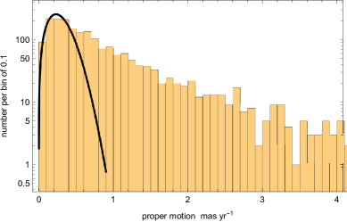
Figure 1: Histograms of absolute (left) and normalized (right) proper motion magnitudes of the RORF sources from the precious set. Note the logarithmic scale of both plots. The black lines show fitted Rayleigh distributions with mean values 0.23 mas yr^-1 on the left and 0.7 on the right, only to assist the eye to distinguish the core distribution and the tail of perturbed values.

Formally, if the VSH functions were orthogonal, and we could ignore the presence of outliers, the residual spin of DR2 with respect to ICRF3 would be $0.23\cdot\sqrt{3/n_{\rm obj}}=8.7$ $\mu$as yr^-1. This is how close we can get to the inertial CRF paradigm with Gaia DR2 in the best case scenario. The number is too large to hope to detect the effect of secular acceleration or signs of propagating primordial gravitational waves. However, a more reliable estimation of uncertainties can be obtained from the full covariance matrices of position and proper motion VSH coefficients.

3 Robustness and confidence of VSH fits

Like numerous other problems of astrometry, and, generally, astronomy, finding a VSH fit to the observed vector field $\boldsymbol{d}$ is an over-determined linear problem, which can be written as

$$\boldsymbol{A}\;\boldsymbol{x}=\boldsymbol{d},$$ (3)

where $\boldsymbol{A}$ is a design matrix, and $\boldsymbol{x}$ is the vector of unknowns, in our case, the coefficients $e_{l}^{m}$ and $h_{l}^{m}$ in arbitrary order, which should be consistent with the order of columns in $\boldsymbol{A}$. This system of equations is most commonly solved by the least-squares method, although other norms of the residual vector could be considered, e.g., a 1-norm solution instead of the 2-norm. The regular 2-norm (least-squares) solution to this problem is

$$\hat{\boldsymbol{x}}=(\boldsymbol{A}^{\prime}\boldsymbol{A})^{-1}\boldsymbol{A}^{\prime}\,\boldsymbol{d}.$$ (4)

The symmetric term of the pseudoinverse matrix $\boldsymbol{C}=(\boldsymbol{A}^{\prime}\boldsymbol{A})^{-1}$ is called the covariance matrix of $\hat{\boldsymbol{x}}$, which contains essential information about the statistical uncertainty of this solution. It is easily verified that if the right-hand part of the system splits into a true vector $\bar{\boldsymbol{d}}$ and a random vector $\boldsymbol{\epsilon}$, whose components are independent variables drawn from ${\cal N}(0,1)$, the expectation $E(\hat{\boldsymbol{x}}\,\hat{\boldsymbol{x}}^{\prime})=\boldsymbol{C}$. The diagonal elements of this matrix are traditionally given high importance, as they are formal variances of the determined parameters. For example, all astrometric catalogs that are in use today list the square roots of the diagonal values as standard deviation errors of the astrometric parameters, while starting with the Hipparcos catalog, the covariances have also been published. Being a useful and intuitively understandable measure of solution quality, the covariance matrix has considerable limitations. It represents the parameters of the statistical distribution of determined parameters reasonably accurately only as long as the above assumptions hold. In practice, they are never realized, as the measurement errors are not normally distributed, nor are they uncorrelated. The single measurement precision is not confidently known, but instead is roughly estimated from shot noise statistics and assumptions about instrumental contributions. In many cases, the calculated covariance has to be scaled by the normalized $\chi^{2}$ statistic from the post-fit residuals (this was implemented in the Gaia mission catalogs, for example). This does not correct the solution for a suboptimal distribution of weights. Furthermore, as we will see in the following, a single realization of the residual vector may significantly deviate from the assumed mean statistics in cases of correlated right-hand parts.

These issues come to the front when we attempt to describe the transformation between the radio and optical reference frames in terms of VSH. Let us consider the singular value decomposition (SVD, Golub & van Loan, 1996) of the design matrix

$$\boldsymbol{A}=\boldsymbol{U}\;\boldsymbol{S}\;\boldsymbol{V}^{\prime}.$$ (5)

The diagonal matrix $\boldsymbol{S}$ includes the singular values of $\boldsymbol{A}$ in decreasing order, $s_{1}\geq s_{2}\geq\ldots\geq s_{m}$, with $m$ the total number of VSH terms in the fit. The least-squares solution is then

$$\hat{\boldsymbol{x}}=\boldsymbol{V}\boldsymbol{S^{\prime}}^{-1}\boldsymbol{U}^{\prime}\,\boldsymbol{d},$$ (6)

and the actual covariance of this solution is

$${\rm Cov}(\hat{\boldsymbol{x}})=E((\hat{\boldsymbol{x}}-\bar{\boldsymbol{x}})(\hat{\boldsymbol{x}}-\bar{\boldsymbol{x}})^{\prime})=\boldsymbol{V}\boldsymbol{S^{\prime}}^{-1}\boldsymbol{U}^{\prime}\;{\rm Cov}(\boldsymbol{d})\;\boldsymbol{U}\boldsymbol{S}^{-1}\boldsymbol{V}^{\prime},$$ (7)

which is equivalent to the previous definition of covariance

$$\boldsymbol{C}=\boldsymbol{V}\;\boldsymbol{S}^{-2}\;\boldsymbol{V}^{\prime}$$ (8)

only if ${\rm Cov}(\boldsymbol{d})$ is identity. Here the square $m\times m$ diagonal matrix $\boldsymbol{S}^{-2}=(\boldsymbol{S}^{\prime}\boldsymbol{S})^{-1}$ is composed of numbers $s_{j}^{-2}$. We are also interested to know how far this solution may deviate from the true parameter vector. We would like to minimize the 2-norm squared of this deviation,

$$r^{2}=(\hat{\boldsymbol{x}}-\bar{\boldsymbol{x}})^{\prime}(\hat{\boldsymbol{x}}-\bar{\boldsymbol{x}})=(\boldsymbol{S}^{\prime-1}\boldsymbol{U}^{\prime}\boldsymbol{\epsilon})^{\prime}(\boldsymbol{S}^{\prime-1}\boldsymbol{U}^{\prime}\boldsymbol{\epsilon}),$$ (9)

where we introduced the error of the right-hand part $\boldsymbol{\epsilon}=\boldsymbol{d}-\bar{\boldsymbol{d}}$. The absolute error of the solution vector is the projection of the right-hand part error onto the basis of singular vectors $\boldsymbol{u}_{i}$, which are the columns of $\boldsymbol{U}$, weighted with the reciprocal singular values $s_{i}^{-1}$. These weights, which define the contribution of different components of the measurement error to the resulting solution error, are key to understanding the properties of the fundamental reference frame tie.

Eq. 9 is valid for any error vector $\boldsymbol{\epsilon}$, including a non-random, or systematic, component. The absolute quadratic error of the frame tie is, generally,

$$r^{2}_{\rm arbitrary}=\sum_{j=1}^{m}s_{j}^{-2}(\boldsymbol{u}_{j}\cdot\boldsymbol{\epsilon})^{2},$$ (10)

where $\boldsymbol{u}_{j}$ are the orthonormal column vectors of $\boldsymbol{U}$. It is straightforward to prove that the largest absolute error is realized on the n-dimensional manifold of unit vectors $\boldsymbol{\epsilon}$ when it coincides with the least significant eigenvector, i.e., $\boldsymbol{\epsilon}=\boldsymbol{u}_{m}$. This is rather improbable for a random data error, but there is a certain probability that $\boldsymbol{\epsilon}$ happens to be rather well aligned with this specific eigenvector. In other words, the absolute error of a least-squares solution with random noise in the data is a random variable itself, and a particular outcome depends on the specific realization of the measurement error.

For a purely random error $\boldsymbol{\epsilon}$ and optimally weighted least-squares problem, the mathematical expectation of $r^{2}$ is

$$E[r^{2}_{\rm random}]=e_{0}^{2}\;\sum_{j=1}^{m}s_{j}^{-2}$$ (11)

with $e_{0}$ denoting the single measurement error of unit weight, i.e., ${\rm var}[\epsilon_{i}]=e_{0}^{2}$, $i=1,\ldots,n$. With respect to random errors in the input data, the accuracy of the frame tie is completely determined by the single measurement error and the spectrum of singular values $s_{j}$. In practice, an additional overhead of solution error is caused by our imperfect knowledge of the measurement variances, i.e., non-optimal weights in the least-squares adjustment.What we usually understand by solution precision or uncertainty of a solution is only the expectation of the average outcome from a great number of trials. In practice, we are given only one trial in most cases, and the solution can be by chance much worse than the expectation even when the usual characteristics, such as the trace of the covariance matrix, appear to be acceptable. Indeed, the same value of trace

$${\rm trace}[{\rm Cov}(\hat{\boldsymbol{x}})]=\sum_{j=1}^{m}s_{j}^{-2}$$ (12)

can be realized when all the singular values are equal, which is the best possible or optimal situation, or a fraction of them are much smaller than the others, resulting in a finite probability of a catastrophically inaccurate solution. Therefore, a metric of solution accuracy and reliability should include not only the range of singular values, which is reflected in the traditional condition number $s_{1}/s_{m}$, but also the greatest singular value itself. The following dimensionless parameter, called robustness of a least-squares solution, is found to represent well the desired uniformity of the singular value spectrum and sensitivity to systematic perturbations in the input data:

$${\cal R}=\frac{\sqrt{n}\,s_{1}^{-1}}{\sqrt{\sum_{j=1}^{m}s_{j}^{-2}}},$$ (13)

where $n$ is the number of condition equations.

This metric can be applied to any astronomical least-squares problems, and can be compared between different applications. It captures the risk of bad solutions due to the spread of singular values, but also reflects the general precision of input data, as well as the number of conditions. For the best possible condition of a unitary matrix $\boldsymbol{A}$, the robustness value becomes ${\cal R}=\sqrt{n}/\sqrt{m}$, which reflects how much the system is overdetermined. This sets the upper bound of robustness, because the value can only be smaller for a non-unitary condition matrix. To achieve a higher robustness, the possible actions are 1) obtain more measurements to increase $n$; 2) minimize the number of unknowns $m$; 3) improve the structure of condition equations by setting up more sensitive measurements (for example, take parallax measurements at the times of maximum parallactic excursion) to minimize the spread of singular values. The robustness parameter captures both the compression of a random component and the chances of particularly poor solutions in the presence of systematic errors.

When using VSH functions to establish the radio-optical frame transformation, we encounter the classic problem of model fitting in astrometry. The series in Eq. 2 is infinite, but the model should be finite, so where do we truncate the series? Would “the more the better” principle work here? Both theory and practice of astrometric data reductions prove this idea to be faulty.

The residual vector $\boldsymbol{\rho}=\boldsymbol{d}-\hat{\boldsymbol{d}}$ is the product of the idempotent matrix $(\boldsymbol{I}-\boldsymbol{U}\,\boldsymbol{U}^{\prime})$ and vector $\boldsymbol{d}$, so that the squared norm of the residual is

$$\boldsymbol{\rho}^{\prime}\,\boldsymbol{\rho}=\boldsymbol{d}^{\prime}(\boldsymbol{I}-\boldsymbol{U}\,\boldsymbol{U}^{\prime})\boldsymbol{d}.$$ (14)

The square idempotent matrix $\boldsymbol{U}\,\boldsymbol{U}^{\prime}$ has a rank of $m$, hence, in the diagonalized form, it is equivalent to $\boldsymbol{Q}\,\boldsymbol{D}\,\boldsymbol{Q}^{\prime}$, with $\boldsymbol{Q}$ being an orthogonal matrix, whose columns are the eigenvectors of the diagonalization mapping, and $\boldsymbol{D}$ a diagonal matrix with exactly $m$ elements equal to 1, and the rest equal to 0. If $\boldsymbol{\epsilon}$, which is the error in $\boldsymbol{d}$, is random and ${\rm Cov}(\boldsymbol{\epsilon})=\boldsymbol{I}$ (due to the optimal weighting of the condition equations), we readily arrive for an unbiased LS solution at the expected squared norm of the post-fit residual vector

$$E[\boldsymbol{\rho}^{\prime}\,\boldsymbol{\rho}]=n-m.$$ (15)

Therefore, the RMS post-fit residual usually declines as $\sqrt{n-m}$ as we include more fitting functions in the model. This behavior is a direct consequence of the independence of the residual norm (Eq. 14) on the singular values $s_{j}$, which specify the actual strength of the conditions, or the compression factors for the eigenvector components of a right-hand side perturbation. By including additional fitting functions in the model, we may get adverse results (i.e., less accurate solution) if these functions provide a weaker condition and result in generally smaller or more dispersed $s_{j}$. The condition factor $\sum_{j=1}^{m}s_{j}^{-2}$, which emerges in the expected absolute error of the parameter vector, Eq. 11, is a viable alternative to post-fit residuals. The well-known statistical $F$-test also provides useful guidance about where to truncate the fitting model. Based on the observation that the quadratic form in Eq. 14 is $\chi^{2}$-distributed due to the mapping matrix being idempotent, one can compare the significance of additional fitting functions in terms of the confidence intervals:

$${\rm Conf}[m_{2},m_{1}]=F_{\rm CDF}\left[\frac{(\chi^{2}_{m_{1}}-\chi^{2}_{m_{2}})(n-m_{2})}{(m_{2}-m_{1})\chi^{2}_{m_{2}}}\right],$$ (16)

where $\chi^{2}_{m}$ is the squared norm of normalized post-fit residuals (Eq. 14) with $m$ fitting functions in the model, $F_{\rm CDF}$ is the standard cumulative distribution function (CDF) for the $F$-distribution, $m_{2}>m_{1}$ are the numbers of terms in the two models under comparison. An improvement in the post-fit residuals is deemed statistically significant if thus calculated ${\rm Conf}[m_{2},m_{1}]$ is greater that a certain limit ${\rm Conf}_{\rm lim}$. One of the shortcomings of this estimate is that the choice of ${\rm Conf}_{\rm lim}$ is somewhat arbitrary, mostly reflecting the subjective tolerance to model overfitting. In practice, the computed CDF often saturates in overdetermined problems, losing the capability to discriminate between alternative models. The other shortcoming is that this statistic is based on the observational residuals and has a weak relation to the accuracy of the solution vector.

4 Functional PCA of the reference frame tie

The spectrum of singular values of the weighted design matrix defines the overall accuracy of a LS solution, as well as the proposed robustness parameter ${\cal R}$ (Eq. 13). It can be explored in a deeper analysis of the quality of the reference frame tie. We note that the projections of the data error vector onto the basis of singular vectors $(\boldsymbol{u}_{j}\cdot\boldsymbol{\epsilon})$ in Eq. 10, which define the absolute error of the solution, are weighted by the reciprocal singular values. Therefore, the greatest value $s_{1}$ identifies the most significant singular vector $\boldsymbol{u}_{1}$, which can be most accurately determined from the given set of data. Conversely, the least significant singular vector is $\boldsymbol{u}_{m}$, and the solution becomes very poor if the data error vector is aligned with it. The singular vectors are conventionally called principal components (PC) of a linear system. In most applications, a few most significant PCs are of interest, because they provide a sufficiently accurate, but less noisy, representation of the observed data set with a given model. In the case under investigation, the singular vectors are linear combinations of vector spherical harmonics, which are vector-valued continuous functions on the unit sphere—thus, the PCs are in fact functions that are orthogonal on the specific set of data points, and their analysis becomes a functional principal component analysis (FPCA).

If we are interested in astrophysical or cosmological applications of the fundamental reference frame, such as the secular acceleration of the Solar system (Kovalevsky, 2003; Kopeikin & Makarov, 2006; Gaia Collaboration et al., 2020) or the presence of primordial gravitational waves, the functional PCA can be applied too. The signal is confined to a certain subset of VSH. The most direct way is to solve the input vector field for that specific set and compute the covariance matrix. However, the resulting uncertainties or the robustness value $\cal{R}$ (Eq. 13) would not account for the potential weakness originating from those principal components of the RORF tie that have large coefficients $s_{j}^{-2}$ but are not explicitly present in the signal estimation. It may be advisable to compute the projections of the given VSH set onto the RORF tie functional PCs and, if necessary, regularize the solution by accepting only the most significant components of this decomposition. The motivation is that any portion of the signal that is carried by the poorly determined RORF tie PCs cannot be trusted to have an acceptable level of input error.

In the context of this paper, the least significant PCs should be identified, because they represent the weakest part of the reference frame tie. Indeed, if $\boldsymbol{\epsilon}=\boldsymbol{u}_{m}$, the error propagates with the factor $s_{m}^{-1}$ into the solution, which may result in substantial error magnification. This dangerous situation becomes especially probable when the model is badly overfitted, i.e., the number of VSH terms is unreasonably high.

4.1 Numerical experiments with Gaia DR2 and ICRF3 data

We start with the “precious set” of 2119 RORF objects selected from the overlap of the ICFR3 and Gaia DR2 catalogs (Makarov et al., 2019). This sample includes only those radio-loud sources from the S/X catalog that have optical counterparts in Gaia DR2 within 3 radii of the combined error ellipse, which corresponds to the 99% confidence level. The selection process also relied on a careful vetting of available high-quality images from the Pan-STARRS and Dark Energy Survey (DES) archives. In view of the unexpectedly large fraction of astrometrically perturbed sources (approaching 1/4), only the best quality data should be used to establish the RORF tie. The results may be crucially sensitive to statistical outliers, as we will see in the following.

A series of LS solutions was produced for the position differences DR2$-$ICRF3 with VSH degrees $L$ between 1 and 8. The number of fitting VSH functions is $m=2(L+1)^{2}-2$. Each object generates two condition equations because of the two-dimensional character of the data. Apart from the position difference fit, a similar solution with the same VSH degree is obtained for Gaia proper motions, which are expected to be zero. For each of these trials, the robustness (Eq. 13) and confidence (Eq. 16) are computed, the latter for $m_{1}=0$, $m_{2}=2(L+1)^{2}-2$, thus estimating the significance of the post-fit reduction in residuals to the input data. The derived confidence levels can then be understood as the probability of rejecting the null hypothesis (that the two reference frames are statistically identical). The magnitude of the fitted vector field is characterized with the median and maximum lengths of the solution vectors on the sample of RORF sources.

The results for the robustness and confidence parameters are presented in Table 1. For the unweighted position differences, the robustness of VSH fits rapidly declines at low degrees, but this behavior slows down by $L=7$ (or $m=126$), where it becomes marginally acceptable. This is to be expected, because as the number of fitting VSH terms increases, the singular values become smaller in general, and the high-degree harmonics cannot be accurately determined from the available data. From this point of view, one would prefer to stay with the lowest possible degrees. The estimated confidence, on the other hand, is not monotonic with $L$, and the most confident fit is obtained at $L=3$. It still falls short of the normally accepted level of 0.99 corresponding to a confident fit. The reason is the presence of a small number of large outliers, which perturb the solution, but continue to show large post-fit residuals. Confident RORF tie solutions cannot be obtained with the original unweighted data even after all the careful filtering and vetting performed in the construction of the precious set.

Table 1: RORF tie solutions for Gaia DR2 and ICRF3

$L$	unweighted positions		weighted positions		weighted proper motions
	Robustness	Confidence	Robustness	Confidence	Robustness	Confidence
1	24.046	0.853	23.450	1.00	22.176	0.760
2	13.461	0.800	12.808	1.00	11.967	0.305
3	9.306	0.976	8.778	1.00	8.216	0.264
4	7.112	0.958	6.602	1.00	6.237	0.016
5	5.276	0.928	5.276	1.00	4.996	0.003
6	4.655	0.952	4.241	1.00	4.095	0.003
7	3.919	0.893	3.504	1.00	3.435	0.001
8	3.368	0.674	3.002	1.00	2.944	0.001

4.2 Empirical weighting schema

Insufficient confidence makes the RORF tie solution ambiguous because it may imply that the two celestial frames are identical within the error of observation, and one could just as well ignore the VSH fits. There are reasons to believe that this is more likely an artifact due to flukes in the data rather than a desired equivalence of the two frames. Although a preliminary version of the ICRF3 catalog was used to align the Gaia DR2 CRF, this adjustment only included the rigid rotation of the Cartesian coordinates, i.e., the three $L=1$ magnetic harmonics. We still find significantly nonzero coefficients for these model terms, which shows how sensitive the result may be to the selection of RORF objects and the weighting principle. The traditional approach of using the formal position uncertainties and covariances (error ellipses) for weights is not well justified in this case. This may only capture the larger expected errors due to faintness of some quasars in the precious set, or a smaller number of available astrometric observations because of the non-uniformity of the scanning schema, but we know that the input positions are commonly perturbed by some kind of “cosmic error”, which is not correlated with these technical circumstances. In establishing a RORF tie, one would like to reduce the impact of this yet unknown error as much as possible. Using the precious set with limited normalized offsets is the first step in this direction. Further improvement can be obtained with a conservative empirical weighting technique based on the tie fitting residuals.

The unweighted VSH solution at a given $L$ is used to compute post-fit residuals, which constitute a discretized vector field on the unit sphere. The magnitude of these vectors depends on $L$ in general, or the rank of the design matrix, as discussed in § 3. The median residual arrow in position, for example, increases from 486 $\mu$as at $L=1$ to 533 $\mu$as at $L=4$, and further to 593 $\mu$as at $L=8$. This happens because a small fraction of objects with discordant and perturbed position differences in the two catalogs pull the unweighted VSH fit and make the rest deviate more from the solution. The median residual vector length $p_{\rm med}$ is computed without weights, and in the next iteration, the weight is defined for $i$th object as

$$w_{i} =1, \>{\rm if}\>p_{i}\leq p_{\rm med}$$

$$=p_{\rm med}/p_{i}, \>{\rm if}\>p_{i}>p_{\rm med}$$

The procedure can be iterated a few times, but numerical experiments showed that the convergence is very fast, and two iterations are usually sufficient. Effectively, this schema down-weights the data points that are less compliant with the smooth tie field, judging them less reliable for a reason that is not a priori known.

The results obtained with this weighting of data are listed in Table 1. The confidence of the tie solutions remarkably improved across the range of VSH degrees, saturating at 1. Hence, the RORF tie leads to a statistically significant reduction of the overall position misalignment between the two reference frames with this weighting schema. Unfortunately, this parameter does not tell us which set of VSH functions represents the tie most accurately. The robustness value still drops with increasing $L$, and it is generally lower than that for the unweighted solution. This interesting outcome may be interpreted in different ways, with one possibility being a degradation of condition through the least significant PCs. As will become clear in the next Section, the weakest condition comes from the distribution of objects on the sky, caused by the irregular coverage of VLBI measurements. The additional perturbation of the RORF objects that contribute the most to the determination of the least significant PCs may be coming from the radio-interferometric side of the input data.

The last two columns in Table 1 give the estimated parameters for the Gaia DR2 proper motion field, for the sake of completeness, although proper motions are not part of the RORF tie. The robustness is slightly smaller for the proper motion fits, which is caused by the smaller number of data points. The most striking result is that the confidence is unacceptable even at the smallest number of fitting terms. In other words, the VSH fit cannot be trusted in any case, because it does not provide the expected reduction in post-fit residuals. This result confirms that the Gaia DR2 proper motion field for ICRF3 objects does not contain any determinable signal of interest, such as the secular aberration or gravitational waves.

4.3 The least significant principal component

As we determined previously, the absolute error of a general LS solution, and of a RORF tie in particular, is defined by the projections of a specific perturbation vector in the input data onto the basis of singular vectors. A catastrophically poor solution can be realized if the perturbation happens to be close to the singular vectors at the end of the range defined by the rank. The least-significant singular vector $\boldsymbol{u}_{m}$ and the corresponding singular value $s_{m}$ are of special interest, therefore, as they define the weakest part of the solution. The smallest singular value decreases with $L$, so that VSH fits with many terms become increasingly risky. This behavior is caused by the presence of irregularities and holes in the sample sky coverage. Indeed, high-degree VSH have many small wiggles on the sphere corresponding to variations of higher spatial frequency. A dearth of data at specific locations makes some of the high-degree model terms poorly conditioned. This also accounts for the rapid decrease of robustness $\cal{R}$ with $L$.

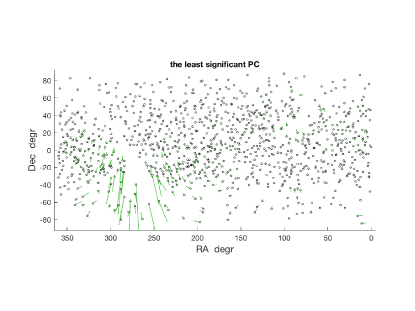
Figure 2: Sky map of the least significant principal component of the RORF tie at degree $L=7$in equatorial coordinates. Small squares mark the position of radio-loud sources from the ICRF3 S/X catalog and their Gaia DR2 counterparts used to establish the tie. The arrows are arbitrarily scaled in length, representing a singular vector field of unit length.

Fig. 2 gives a graphical presentation of the RORF tie least significant principal component (with empirical weighting as described in § 4.2) at $L=7$. The robustness of this solution is just above 3.5 (Table 1), so it is deemed the highest degree fit that is still acceptable. The arrows show arbitrarily scaled values of $\boldsymbol{u}_{126}$ for half of the sample, to avoid overcrowding. The small circles represent the source positions, i.e., the arrows’ origins. The corresponding singular value is $s_{126}=15.2$, which indicates a nice degree of measurement error shrinkage in the VSH fit even for this component. The graph reveals that the weakest component of the Gaia-ICRF3 tie is confined to a specific area in the southern hemisphere, where the density of ICRF3 is much lower, and a fairly large hole around the Galactic center.

5 Conclusions

A wide range of basic research projects in astronomy, cosmology, and physics, as well as practical application in geodesy and navigation, require position and motion determinations in the two fundamental reference frames. The consistency of these frames is absolutely essential, and the transformation of coordinates between the frames, called the radio-optical reference frame tie, should be established and registered as accurately as possible. On the example of the Gaia DR2 and ICRF3 S/X catalogs, it is shown in this paper, that a confident solution can be obtained after a careful two-stage vetting of the available RORF sources. The first step is to minimize the impact of the cosmic error, which affects at least 25% of the sample, and may be caused by the internal structure of beamed radio jets (Petrov et al., 2019), optical offsets of AGNs from the host galaxy’s centers, morphology of nearby galaxies, unresolved duplicity, gravitational lensing, and other phenomena. The second step is to empirically downweight the remaining perturbations, which distort the functional fit, generate larger median post-fit residuals, and drive the confidence of global solutions to below the acceptable levels.

The newly introduced robustness parameter and the $F$-test confidence are helpful in determining the highest degree of the VSH model, which provides the finest detail of the functional representation, while remaining reasonably accurate and robust. It is demonstrated that the degree should not be larger than $L=7$ for the two investigated catalogs. The choice of a lower degree is a trade-off between the desired robustness of the tie and the small scale fidelity in applications limited to specific regions of the celestial sphere. In the context of general alignment of the two fundamental celestial reference frames, when the best result at various spatial scales is desired, the recommended degree is 6 or 7 for ICRF3 and Gaia DR2. This number may change upwards for the future Gaia, and, eventually, ICRF versions as the quality of astrometric data improves.

The least significant functional principal component of the RORF tie demonstrates the weakest point, through which the largest possible error can be realized. It is a specific vector field on the celestial sphere, and its largest vectors are limited to well-defined areas of the sky, mostly situated in the southern hemisphere close to the Galactic plane and the Galactic center. Clearly, the weakness is caused by the dearth of ICRF3 sources in the south, and the smaller density of optical counterparts in Gaia due to crowding and extinction. The situation can be improved by prioritizing the planned extension of ICRF defining sample in the southern hemisphere according to the distribution of the least significant PC. The Gaia processing consortium may also consider making a special effort of windowing known ICRF counterparts closer to the Galactic plane.

The Gaia DR2 proper motion field of the selected ICRF3 sources, on the other hand, does not contain any statistically significant signal, so no transformation for the spin is required. This is to be expected, to some extent, because the Gaia proper motion rigid rotation was adjusted on a much greater sample of infrared-detected quasars and AGNs (Mignard et al., 2016). The absence of significant higher-degree terms testifies to the good quality of astrometric calibration of time-dependent parameters; on the other hand, the modest accuracy of the proper motion VSH fit precludes astrophysical exploration of these data.

6 Acknowledgments

The author is grateful to Dr. Brian Luzum and the anonymous referee, whose comments and corrections helped to improve the paper. This work has made use of data from the European Space Agency (ESA) mission Gaia (http://www.cosmos.esa.int/gaia), processed by the Gaia Data Processing and Analysis Consortium (DPAC,
http://www.cosmos.esa.int/web/gaia/dpac/consortium). Funding for the DPAC has been provided by national institutions, in particular the institutions participating in the Gaia Multilateral Agreement.

References

- Brosche (1966) Brosche, P. 1966, Veröffentlichungen des Astronomischen Rechen-Instituts Heidelberg, 17, 1
- Brown & Gaia Collaboration (2018) Brown, A. G. A., Vallenari, A., Prusti, T., and Gaia Collaboration, 2018, A&A, 616, A1
- Charlot et al. (2020) Charlot, P., Jacobs, C. S., Gordon, D., et al. 2020, arXiv:2010.13625
- Dette et al. (2005) Dette, H., Melas, V. B., Pepelyshev, A. 2005, The Annals of Statistics, 33, 2758, doi:10.1214/009053605000000552
- Downes et al. (2012) Downes, T. P., Welch, D., Scott, K. S., et al. 2012, MNRAS, 423, 529. doi:10.1111/j.1365-2966.2012.20896.x
- Gaia Collaboration et al. (2018) Gaia Collaboration, Mignard, F., Klioner, S. A., et al. 2018, A&A, 616, A14. doi:10.1051/0004-6361/201832916
- Golub & van Loan (1996) Golub, G.H., van Loan, C.F. 1996, Matrix Computations, The John Hopkins University Press
- Hamilton et al. (2008) Hamilton, T.S., Casertano, S., Turnshek, D.A. 2008, ApJ, 678, 22.
- He et al. (2018) He, S., Wang, L., & Huang, J. Z. 2018, ApJ, 857, 110. doi:10.3847/1538-4357/aab0a8
- Gaia Collaboration et al. (2020) Gaia Collaboration, Klioner, S. A., Mignard, F., et al. 2020, arXiv:2012.02036
- Kopeikin & Makarov (2006) Kopeikin, S.M., Makarov, V.V., AJ, 131, 1471
- Kovalevsky (2003) Kovalevsky, J. 2003, A&A, 404, 743
- Lindegren et al. (2018) Lindegren, L., Hernández, J., Bombrun, A., et al. 2018, A&A, 616, A2
- Makarov & Milman (2005) Makarov, V. V. & Milman, M. 2005, PASP, 117, 757
- Makarov & Murphy (2007) Makarov, V. V. & Murphy, D. W. 2007, AJ, 134, 367
- Makarov et al. (2012) Makarov, V. V., Dorland, B. N., Gaume, R. A., et al. 2012, AJ, 144, 22
- Makarov et al. (2012) Makarov, V.V., Berghea, C., Boboltz, D., et al. 2012, MmSAI, 83, 952
- Makarov et al. (2017) Makarov, V. V., Frouard, J., Berghea, C. T., et al. 2017, ApJ, 835, L30. doi:10.3847/2041-8213/835/2/L30
- Makarov et al. (2019) Makarov, V. V., Berghea, C. T., Frouard, J., et al. 2019, ApJ, 873, 132
- Mignard & Klioner (2012) Mignard, F., & Klioner, S. 2012, A&A, 547, A59
- Mignard et al. (2016) Mignard, F., Klioner, S., Lindegren, L., et al. 2016, A&A, 595, 5
- Petrov & Kovalev (2017) Petrov, L. & Kovalev, Y. Y. 2017, MNRAS, 471, 3775. doi:10.1093/mnras/stx1747
- Petrov et al. (2019) Petrov, L., Kovalev, Y.Y., Plavin, A.V. 2018, MNRAS, 482, 3023
- Plavin et al. (2019) Plavin, A. V., Kovalev, Y. Y., Pushkarev, A. B., et al. 2019, MNRAS, 485, 1822
- Prusti et al. (2016) Prusti, T., de Bruijne, J.H.J., Brown, A.G.A., et al. 2016, A&A, 595, 1