Reproducibility Report
Rigging the Lottery: Making All Tickets Winners

Reproducibility Summary

Scope of Reproducibility

For a fixed parameter count and compute budget, the proposed algorithm (RigL) claims to directly train sparse networks that match or exceed the performance of existing dense-to-sparse training techniques (such as pruning). RigL does so while requiring constant Floating Point Operations (FLOPs) throughout training. The technique obtains state-of-the-art performance on a variety of tasks, including image classification and character-level language-modelling.

Methodology

We implement RigL from scratch in Pytorch using boolean masks to simulate unstructured sparsity. We rely on the description provided in the original paper, and referred to the authors’ code for only specific implementation detail such as handling overflow in ERK initialization. We evaluate sparse training using RigL for WideResNet-22-2 on CIFAR-10 and ResNet-50 on CIFAR-100, requiring 2 hours and 6 hours respectively per training run on a GTX 1080 GPU.

Results

We reproduce RigL’s performance on CIFAR-10 within 0.1% of the reported value. On both CIFAR-10/100, the central claim holds—given a fixed training budget, RigL surpasses existing dynamic-sparse training methods over a range of target sparsities. By training longer, the performance can match or exceed iterative pruning, while consuming constant FLOPs throughout training. We also show that there is little benefit in tuning RigL’s hyper-parameters for every sparsity, initialization pair—the reference choice of hyperparameters is often close to optimal performance.

Going beyond the original paper, we find that the optimal initialization scheme depends on the training constraint. While the Erdos-Renyi-Kernel distribution outperforms Random distribution for a fixed parameter count, for a fixed FLOP count, the latter performs better. Finally, redistributing layer-wise sparsity while training can bridge the performance gap between the two initialization schemes, but increases computational cost.

What was easy

The authors provide code for most of the experiments presented in the paper. The code was easy to run and allowed us to verify the correctness of our re-implementation. The paper also provided a thorough and clear description of the proposed algorithm without any obvious errors or confusing exposition.

What was difficult

Tuning hyperparameters involved multiple random seeds and took longer than anticipated. Verifying the correctness of a few baselines was tricky and required ensuring that the optimizer’s gradient (or momentum) buffers were sparse (or dense) as specified by the algorithm. Compute limits restricted us from evaluating on larger datasets such as Imagenet.

Communication with original authors

We had responsive communication with the original authors, which helped clarify a few implementation and evaluation details, particularly regarding the FLOP counting procedure.

1 Introduction

Sparse neural networks are a promising alternative to conventional dense networks—having comparatively greater parameter efficiency and lesser floating-point operations (FLOPs) (Han et al. [2016], Ashby et al. [2017], Srinivas et al. [2017]). Unfortunately, present techniques to produce sparse networks of commensurate accuracy involve multiple cycles of training dense networks and subsequent pruning. Consequently, such techniques offer no advantage over training dense networks, either computationally or memory-wise.

In the paper Evci et al. [2020], the authors propose RigL, an algorithm for training sparse networks from scratch. The proposed method outperforms both prior art in training sparse networks, as well as existing dense-to-sparse training algorithms. By utilising dense gradients only during connectivity updates and avoiding any global sparsity redistribution, RigL can maintain a fixed computational cost and parameter count throughout training.

As a part of the ML Reproducibility Challenge, we replicate RigL from scratch and investigate if dynamic-sparse training confers significant practical benefits compared to existing sparsifying techniques.

2 Scope of reproducibility

In order to verify the central claims presented in the paper we focus on the following target questions:

• Does RigL outperform existing sparse-to-sparse training techniques—such as SET (Mocanu et al. [2018]) and SNFS (Dettmers and Zettlemoyer [2020])—and match the accuracy of dense-to-sparse training methods such as iterative pruning (Zhu and Gupta [2018])?

• RigL requires two additional hyperparameters to tune. We investigate the sensitivity of final performance to these hyperparameters across a variety of target sparsities (Section 5.3).

• How does the choice of sparsity initialization affect the final performance for a fixed parameter count and a fixed training budget (Section 6.1)?

• Does redistributing layer-wise sparsity during connection updates (Dettmers and Zettlemoyer [2020]) improve RigL’s performance? Can the final layer-wise distribution serve as a good sparsity initialization scheme (Section 6.2)?

3 Methodology

The authors provide publicly accessible code written in Tensorflow (Abadi et al. [2016]). To gain a better understanding of various implementation aspects, we opt to replicate RigL in Pytorch (Paszke et al. [2019]). Our implementation extends the open-source code of Dettmers and Zettlemoyer [2020] which uses a boolean mask to simulate unstructured sparsity. Our source code is publicly accessible on Github with training plots available on WandB (Biewald [2020]).

Mask Initialization

For a network with $L$ layers and total parameters $N$, we associate each layer with a random boolean mask of sparsity $s_{l},\;l\in[L]$. The overall sparsity of the network is given by $S=\frac{\sum_{l}s_{l}N_{l}}{N}$, where $N_{l}$ is the parameter count of layer $l$. Sparsities $s_{l}$ are determined by the one of the following mask initialization strategies:

• Uniform: Each layer has the same sparsity, i.e., $s_{l}=S\;\forall l$. Similar to the original authors, we keep the first layer dense in this initialization.

• Erdos-Renyi (ER): Following Mocanu et al. [2018], we set $s_{l}\propto\left(1-\frac{C_{\text{in}}+C_{\text{out}}}{C_{\text{in}}\times C_{\text{out}}}\right)$, where $C_{\text{in}},C_{\text{out}}$ are the in and out channels for a convolutional layer and input and output dimensions for a fully-connected layer.

• Erdos-Renyi-Kernel (ERK): Modifies the sparsity rule of convolutional layers in ER initialization to include kernel height and width, i.e., $s_{l}\propto\left(1-\frac{C_{\text{in}}+C_{\text{out}}+w+h}{C_{\text{in}}\times C_{\text{out}}\times w\times h}\right)$, for a convolutional layer with $C_{\text{in}}\times C_{\text{out}}\times w\times h$ parameters.

We do not sparsify either bias or normalization layers, since these have a negligible effect on total parameter count.

Mask Updates

Every $\Delta T$ training steps, certain connections are discarded, and an equal number are grown. Unlike SNFS (Dettmers and Zettlemoyer [2020]), there is no redistribution of layer-wise sparsity, resulting in constant FLOPs throughout training.

Pruning Strategy

Similar to SET and SNFS, RigL prunes $f$ fraction of smallest magnitude weights in each layer. As detailed below, the fraction $f$ is decayed across mask update steps, by cosine annealing:

$$f(t)=\frac{\alpha}{2}\left(1+\cos\left(\frac{t\pi}{T_{\text{end}}}\right)\right)$$ (1)

where, $\alpha$ is the initial pruning rate and $T_{\text{end}}$ is the training step after which mask updates are ceased.

Growth Strategy

RigL’s novelty lies in how connections are grown: during every mask update, $k$ connections having the largest absolute gradients among current inactive weights (previously zero + pruned) are activated. Here, $k$ is chosen to be the number of connections dropped in the prune step. This requires access to dense gradients at each mask update step. Since gradients are not accumulated (unlike SNFS), RigL does not require access to dense gradients at every step. Following the paper, we initialize newly activated weights to zero.

4 Experimental Settings

4.1 Model descriptions

For experiments on CIFAR-10 (Alex Krizhevsky [2009]), we use a Wide Residual Network (Zagoruyko and Komodakis [2016]) with depth 22 and width multiplier 2, abbreviated as WRN-22-2. For experiments on CIFAR-100 (Alex Krizhevsky [2009]), we use a modified variant of ResNet-50 (He et al. [2016]), with the initial $7\times 7$ convolution replaced by two $3\times 3$ convolutions (architecture details provided in the supplementary material).

4.2 Datasets and Training descriptions

We conduct our experiments on the CIFAR-10 and CIFAR-100 image classification datasets. For CIFAR-10, we use a train/val/test split of 45k/5k/10k samples. In comparison, the authors use no dedicated validation set, with 50k samples and 10k samples comprising the train set and test set, respectively. This causes a slight performance discrepancy between our reproduction and the metrics reported by the authors (dense baseline has a test accuracy of 93.4% vs 94.1% reported). However, our replication matches the paper’s performance when 50k samples are used for the train set (Table 4). We use a validation split of 10k samples for CIFAR-100 as well.

Table 1: Test accuracy of reference and our implementations on CIFAR-10, tabulated for three different sparsities. Note that the runs listed here do not use a separate validation set while training.

Method	Ours			Original
Dense	94.6			94.1
	$1-s=0.1$	$1-s=0.2$	$1-s=0.5$	$1-s=0.1$	$1-s=0.2$	$1-s=0.5$
Static (ERK)	91.6	93.2	94.3	91.6	92.9	94.2
Pruning	93.2	93.6	94.3	93.3	93.5	94.1
RigL (ERK)	93.2	93.8	94.4	93.1	93.8	94.3

On both datasets, we train models for 250 epochs each, optimized by SGD with momentum. Our training pipeline uses standard data augmentation, which includes random flips and crops. When training on CIFAR-100, we additionally include a learning rate warmup for 2 epochs and label smoothening of 0.1 (Goyal et al. [2017]). We also initialize the last batch normalization layer (Ioffe and Szegedy [2015]) in each BottleNeck block to 0, following He et al. [2019].

4.3 Hyperparameters

RigL includes two additional hyperparameters ($\alpha,\Delta T$) in comparison to regular dense network training. In Sections 5.1 and 5.2, we set $\alpha=0.3,\Delta T=100$, based on the original paper. Optimizer specific hyperparameters—learning rate, learning rate schedule, and momentum—are also set according to the original paper. In Section 5.3, we tune these hyperparameters with Optuna (Akiba et al. [2019]). We also examine whether indivdually tuning the learning rate for each sparsity value offers any significant benefit.

4.4 Baseline implementations

We compare RigL against various baselines in our experiments: SET (Mocanu et al. [2018]), SNFS (Dettmers and Zettlemoyer [2020]), and Magnitude-based Iterative-pruning (Zhu and Gupta [2018]). We also compare against two weaker baselines, viz., Static Sparse training and Small-Dense networks. The latter has the same structure as the dense model but uses fewer channels in convolutional layers to lower parameter count. We implement iterative pruning with the pruning interval kept same as the masking interval for a fair comparison.

4.5 Computational requirements

We run our experiments on a SLURM cluster node—equipped with 4 NVIDIA GTX1080 GPUs and a 32 core Intel CPU. Each experiment on CIFAR-10 and CIFAR-100 consumes about 1.6 GB and 7 GB of VRAM respectively and is run for 3 random seeds to capture performance variance. We require about 6 and 8 days of total compute time to produce all results, including hyper-parameter sweeps and extended experiments, on CIFAR-10 and CIFAR-100 respectively.

5 Results

Given a fixed training FLOP budget, RigL surpasses existing dynamic sparse training methods over a range of target sparsities, on both CIFAR-10 and 100 (Sections 5.1, 5.2). By training longer, RigL matches or marginally outperforms iterative pruning. However, unlike pruning, its FLOP consumption is constant throughout. This a prime reason for using sparse networks, and makes training larger networks feasible. Finally, as evaluated on CIFAR-10, the original authors’ choice of hyper-parameters are close to optimal for multiple target sparsities and initialization schemes (Section 5.3).

5.1 WideResNet-22 on CIFAR-10

Table 2: WideResNet-22-2 on CIFAR10, tabulated for two density $(1-s)$ values. We group methods by their FLOP requirement and in each group, we mark the best accuracy in bold. Similar to Evci et al. [2020], we assume that algorithms utilize sparsity during training. All results are obtained by methods implemented in our unified codebase.

Method	$\mathbf{1-s=0.1}$		$\mathbf{1-s=0.2}$
	Accuracy $\uparrow$ (Test)	FLOPs $\downarrow$ (Train, Test)	Accuracy $\uparrow$ (Test)	FLOPs $\downarrow$ (Train, Test)
Small Dense	89.0 $\pm$ 0.35	0.11x, 0.11x	91.0 $\pm$ 0.07	0.20x, 0.20x
Static	89.1 $\pm$ 0.17	0.10x, 0.10x	91.2 $\pm$ 0.16	0.20x,0.20x
SET	91.3 $\pm$ 0.47	0.10x, 0.10x	92.7 $\pm$ 0.28	0.20x, 0.20x
RigL	91.7 $\pm$ 0.18	0.10x, 0.10x	92.6 $\pm$ 0.10	0.20x, 0.20x
SET (ERK)	92.2 $\pm$ 0.04	0.17x, 0.17x	92.9 $\pm$ 0.16	0.35x, 0.35x
RigL (ERK)	92.4 $\pm$ 0.06	0.17x, 0.17x	93.1 $\pm$ 0.09	0.35x, 0.35x
Static$2\times$	89.15 $\pm$ 0.17	0.20x, 0.10x	91.2 $\pm$ 0.16	0.40x, 0.20x
Lottery	90.4 $\pm$ 0.09	0.45x, 0.13x	92.0 $\pm$ 0.31	0.68x,0.27x
SET$2\times$	83.3 $\pm$ 15.33	0.20x, 0.10x	93.0 $\pm$ 0.22	0.41x, 0.20x
SNFS	92.4 $\pm$ 0.43	0.51x, 0.27x	92.7 $\pm$ 0.20	0.66x, 0.49x
SNFS (ERK)	92.2 $\pm$ 0.2	0.52x, 0.28x	92.8 $\pm$ 0.07	0.66x, 0.49x
SNFS$2\times$	92.3 $\pm$ 0.33	1.02x, 0.27x	93.2 $\pm$ 0.14	1.32x, 0.98x
RigL$2\times$	92.3 $\pm$ 0.25	0.20x, 0.10x	93.0 $\pm$ 0.21	0.41x, 0.20x
Pruning	92.6 $\pm$ 0.08	0.32x,0.13x	93.2 $\pm$ 0.27	0.41x,0.27x
RigL$2\times$ (ERK)	92.7 $\pm$ 0.37	0.34x, 0.17x	93.3 $\pm$ 0.09	0.70x, 0.35x
Dense Baseline	93.4 $\pm$ 0.07	9.45e8, 3.15e8	-	-

Results on the CIFAR-10 dataset are provided in Table 2. Tabulated metrics are averaged across 3 random seeds and reported with their standard deviation. All sparse networks use random initialization, unless indicated otherwise.

While SET improves over the performance of static sparse networks and small-dense networks, methods utilizing gradient information (SNFS, RigL) obtain better test accuracies. SNFS can outperform RigL, but requires a much larger training budget, since it (a) requires dense gradients at each training step, (b) redistributes layer-wise sparsity during mask updates. For all sparse methods, excluding SNFS, using ERK initialization improves performance, but with increased FLOP consumption. We calculate theoretical FLOP requirements in a manner similar to Evci et al. [2020] (exact details in the supplementary material).

Figure 1 contains test accuracies of select methods across two additional sparsity values: ($0.5,0.95$). At lower sparsities (higher densities), RigL matches the performance of the dense baseline. Performance further improves by training for longer durations. Particularly, training RigL (ERK) twice as long at 90% sparsity exceeds the performance of iterative pruning while requiring similar theoretical FLOPs. This validates the original authors’ claim that RigL (a sparse-to-sparse training method) outperforms pruning (a dense-to-sparse training method).

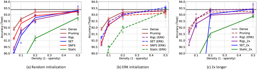
Figure 1: Test Accuracy vs Sparsity on CIFAR-10, plotted for Random initialization (left), ERK initialization (center), and for training $2\times$ longer (right). Owing to random growth, SET can be unstable when training for longer durations with higher sparsities. Overall, RigL_$2\times$ (ERK) achieves highest test accuracy.

5.2 ResNet-50 on CIFAR100

[figure]entry for figure Table 3: Benchmarking sparse ResNet-50s on CIFAR-100, tabulated by performance and cost (below), and plotted across densities (right). In each group below, RigL outperforms or matches existing sparse-to-sparse and dense-to-sparse methods. Notably, RigL$3\times$ at 90% sparsity and RigL$2\times$ at 80% sparsity surpass iterative pruning with similar FLOP consumption. RigL$2\times$ (ERK) further improves performance but requires a larger training budget. Method $\mathbf{1-s=0.1}$ $\mathbf{1-s=0.2}$ Accuracy $\uparrow$ (Test) FLOPs $\downarrow$ (Train, Test) Accuracy $\uparrow$ (Test) FLOPs $\downarrow$ (Train, Test) Static 69.7 $\pm$ 0.42 0.10x, 0.10x 72.3 $\pm$ 0.30 0.20x,0.20x Small Dense 70.8 $\pm$ 0.22 0.11x, 0.11x 72.6$\pm$ 0.93 0.20x, 0.20x SET 71.4 $\pm$ 0.35 0.10x, 0.10x 73.4 $\pm$ 0.45 0.20x, 0.20x RigL 71.8 $\pm$ 0.33 0.10x, 0.10x 73.5 $\pm$ 0.04 0.20x, 0.20x Static (ERK) 71.5 $\pm$ 0.18 0.22x, 0.22x 73.2 $\pm$ 0.39 0.38x, 0.38x SET (ERK) 72.3 $\pm$ 0.39 0.22x, 0.22x 73.5 $\pm$ 0.25 0.38x, 0.38x RigL (ERK) 72.6 $\pm$ 0.37 0.23x, 0.22x 73.4 $\pm$ 0.15 0.38x, 0.38x SNFS 72.3 $\pm$ 0.20 0.58x, 0.37x 73.9 $\pm$ 0.20 0.70x, 0.55x SNFS (ERK) 73.0 $\pm$ 0.33 0.59x, 0.38x 73.9 $\pm$ 0.27 0.69x, 0.54x Pruning 73.1 $\pm$ 0.32 0.36x,0.11x 73.8 $\pm$ 0.23 0.45x,0.25x RigL$2\times$ 73.1 $\pm$ 0.71 0.20x, 0.10x 74.0 $\pm$ 0.24 0.41x, 0.20x Lottery 73.6 $\pm$ 0.32 0.62x,0.11x 74.2 $\pm$ 0.41 0.81x,0.25x RigL$3\times$ 73.7 $\pm$ 0.16 0.30x, 0.10x 74.2 $\pm$ 0.23 0.61x, 0.20x RigL$2\times$ (ERK) 73.6 $\pm$ 0.05 0.46x, 0.22x 74.4 $\pm$ 0.10 0.76x, 0.38x Dense Baseline 74.7 $\pm$ 0.38 7.77e9, 2.59e9 - -

We see similar trends when training sparse variants of ResNet-50 on the CIFAR-100 dataset (Table 5.2, metrics reported as in Section 5.1). We also include a comparison against sparse networks trained with the Lottery Ticket Hypothesis (Frankle and Carbin [2018]) in Table 5.2—we obtain tickets with a commensurate performance for sparsities lower than 80%. Finally, the choice of initialization scheme affects the performance and FLOP consumption by a greater extent than the method used itself, with the exception of SNFS (groups 1 and 2 in Table 5.2).

5.3 Hyperparameter Tuning

Table 4: Reference vs Optimal $(\alpha,\Delta T)$ on CIFAR-10. Optimal hyperparameters are obtained by tuning with a TPE sampler in Optuna. The difference between the reference and optimal performance is small, indicating that there is not a significant benefit in tuning $(\alpha,\Delta T)$ individually for each initialization and sparsity configuration.

Initialization	Density	Reference		Optimal
	$(1-s)$	$(\alpha,\Delta T)$	Accuracy $\uparrow$ (Test)	$(\alpha,\Delta T)$	Accuracy $\uparrow$ (Test)
Random	0.1	0.3, 100	91.7 $\pm$ 0.18	0.197, 50	91.8 $\pm$ 0.17
Random	0.2	0.3, 100	92.6 $\pm$ 0.10	0.448, 150	92.8 $\pm$ 0.16
Random	0.5	0.3, 100	93.3 $\pm$ 0.07	0.459, 550	93.3 $\pm$ 0.18
ERK	0.1	0.3, 100	92.4 $\pm$ 0.06	0.416, 200	92.4 $\pm$ 0.23
ERK	0.2	0.3, 100	93.1 $\pm$ 0.09	0.381, 950	93.1 $\pm$ 0.21
ERK	0.5	0.3, 100	93.4 $\pm$ 0.14	0.287, 500	93.8 $\pm$ 0.06

$(\alpha,\Delta T)$ vs Sparsities

To understand the impact of the two additional hyperparameters included in RigL, we use a Tree of Parzen Estimator (TPE sampler, Bergstra et al. [2011]) via Optuna to tune $(\alpha,\Delta T)$. We do this for sparsities $(1-s)\in\{0.1,0.2,0.5\}$, and a fixed learning rate of $0.1$. Additionally, we set the sampling domain for $\alpha$ and $\Delta T$ as $[0.1,0.6]$ and $\{50,100,150,...,1000\}$ respectively. We use 15 trials for each sparsity value, with our objective function as the validation accuracy averaged across 3 random seeds.

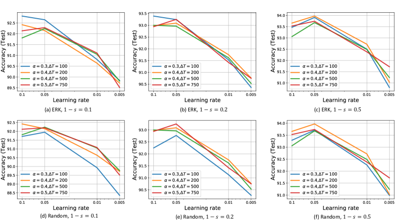
Figure 2: Learning Rate vs Sparsity on CIFAR-10. Runs using a learning rate $>0.1$ do not converge and are not plotted here. There is little benefit in tuning the learning rate for each sparsity, and $0.1,0.05$ are good choices overall.

Table 4 shows the test accuracies of tuned hyperparameters. While the reference hyperparameters (original authors, $\alpha=0.3,\Delta T=100$) differ from the obtained optimal hyperparameters, the difference in performance is marginal, especially for ERK initialization. This in agreement with the original paper, which finds $\alpha\in\{0.3,0.5\},\Delta T=100$ to be suitable choices. We include contour plots detailing the hyperparameter trial space in the supplementary material.

Learning Rate vs Sparsities

We further examine if the final performance improves by tuning the learning rate ($\eta$) individually for each sparsity-initialization pair. We employ a grid search over $\eta\in\{0.1,0.05,0.01,0.005\}$ and $(\alpha,\Delta T)\in\{(0.3,100),(0.4,200),(0.4,500),(0.5,750)\}$. As seen in Figure 2, $\eta=0.1$ and $\eta=0.05$ are close to optimal values for a wide range of sparsities and initializations. Since these learning rates also correspond to good choices for the Dense baseline, one can employ similar values when training with RigL.

6 Results beyond Original Paper

6.1 Sparsity Distribution vs FLOP Consumption

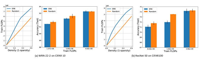
Figure 3: Test Accuracy vs FLOP consumption of WideResNet-22-2 on CIFAR-10 and ResNet-50 on CIFAR-100, compared for Random and ERK initializations. For the same FLOP budget, models trained with ERK initialization must be more sparse, resulting in inferior performance.

While ERK initialization outperforms Random initialization consistently for a given target parameter count, it requires a higher FLOP budget. Figure 3 compares the two initialization schemes across fixed training FLOPs. Theoretical FLOP requirement for Random initialization scales linearly with density $(1-s)$, and is significantly lesser than ERK’s FLOP requirements. Consequently, Random initialization outperforms ERK initialization for a given training budget.

6.2 Effect of Redistribution

Table 5: Effect of redistribution during RigL updates, evaluated on CIFAR10 and CIFAR100. By utilising sparse gradient or sparse momentum based redistribution, RigL (Random) matches RigL (ERK)’s performance. Among Random and ERK initialized experiments, we mark the best metrics under each sparsity and dataset in bold.

Method	Redistribution	CIFAR-10				CIFAR-100
		$1-s=0.1$		$1-s=0.2$		$1-s=0.1$		$1-s=0.2$
		Accuracy $\uparrow$ (Test)	FLOPs $\downarrow$ (Train, Test)	Accuracy $\uparrow$ (Test)	FLOPs $\downarrow$ (Train, Test)	Accuracy $\uparrow$ (Test)	FLOPs $\downarrow$ (Train, Test)	Accuracy $\uparrow$ (Test)	FLOPs $\downarrow$ (Train, Test)
Random Initialization
RigL	-	91.7 $\pm$ 0.18	0.10x, 0.10x	92.9 $\pm$ 0.10	0.20x, 0.20x	71.8 $\pm$ 0.33	0.10x, 0.10x	73.5 $\pm$ 0.04	0.20x, 0.20x
RigL-SG	Sparse Grad	92.2 $\pm$ 0.17	0.28x, 0.28x	92.7 $\pm$ 0.25	0.49x, 0.49x	72.3 $\pm$ 0.12	0.36x,0.35x	73.7 $\pm$ 0.15	0.53x, 0.53x
RigL-SM	Sparse Mmt	92.2 $\pm$ 0.20	0.28x, 0.28x	92.9 $\pm$ 0.21	0.50x, 0.49x	72.6 $\pm$ 0.27	0.36x,0.36x	73.7 $\pm$ 0.35	0.53x, 0.53x
ERK Initialization
RigL	-	92.4 $\pm$ 0.06	0.17x, 0.17x	93.1 $\pm$ 0.09	0.35x, 0.35x	72.6 $\pm$ 0.37	0.23x, 0.22x	73.4 $\pm$ 0.15	0.38x, 0.38x
RigL-SG	Sparse Grad	92.1 $\pm$ 0.19	0.28x, 0.28x	92.7 $\pm$ 0.19	0.49x, 0.49x	73.0 $\pm$ 0.13	0.37x,0.36x	74.2 $\pm$ 0.26	0.53x, 0.53x
RigL-SM	Sparse Mmt	92.27 $\pm$ 0.01	0.28x, 0.28x	93.0 $\pm$ 0.13	0.50x, 0.49x	72.6 $\pm$ 0.27	0.37x, 0.37x	74.2 $\pm$ 0.13	0.53x, 0.53x
Re-Initialization with RigL-SM (Random, ERK)
RigL	-	90.3 $\pm$ 0.34	0.28x, 0.28x	91.0 $\pm$ 0.38	0.50x, 0.49x	67.6 $\pm$ 0.28	0.36x, 0.36x	68.9 $\pm$ 0.65	0.53x, 0.53x
RigL (ERK)	-	90.2 $\pm$ 0.57	0.28x, 0.28x	90.6 $\pm$ 0.56	0.50x, 0.49x	67.8 $\pm$ 0.73	0.37x, 0.37x	68.9 $\pm$ 0.47	0.53x, 0.53x

One of the main differences of RigL over SNFS is the lack of layer-wise redistribution during training. We examine if using a redistribution criterion can be beneficial and bridge the performance gap between Random and ERK initialization. Following Dettmers and Zettlemoyer [2020], during every mask update, we reallocate layer-wise density proportional to its average sparse gradient or momentum (RigL-SG, RigL-SM).

Table 5 shows that redistribution significantly improves RigL (Random), but not RigL (ERK). We additionally plot the FLOP requirement against training steps and the final sparsity distribution in Figure 4. The layer-wise sparsity distribution largely becomes constant within a few epochs. The final distribution is similar, but more “extreme” than ERK—wherever ERK exceeds/falls short of Random, redistribution does so by a greater extent.

By allocating higher densities to $1\times 1$ convolutions (convShortcut in Figure 4), redistribution significantly increases the FLOP requirement—and hence, is not a preferred alternative to ERK. Surprisingly, initializing RigL with the final sparsity distribution in a manner similar to the Lottery Ticket Hypothesis results in subpar performance (group 3, Table 5).

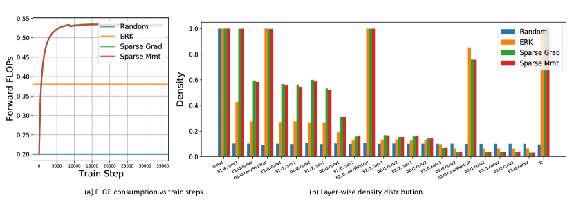
Figure 4: Effect of redistribution on RigL’s performance, evaluated using WideResNet-22-2 on CIFAR10 at 80% sparsity. (left) FLOPs required per forward pass, shown relative to the dense baseline, rises quickly and saturates within a few epochs (~10k steps) for both sparse gradient and sparse momentum based redistribution. (right) Comparison of the final density distribution against Random and ERK counterparts. “b” refers to block and “l” layer here.

7 Discussion

Evaluated on image classification, the central claims of Evci et al. [2020] hold true—RigL outperforms existing sparse-to-sparse training methods and can also surpass other dense-to-sparse training methods with extended training. RigL is fairly robust to its choice of hyperparameters, as they can be set independent of sparsity or initialization. We find that the choice of initialization has a greater impact on the final performance and compute requirement than the method itself. Considering the performance boost obtained by redistribution, proposing distributions that attain maximum performance given a FLOP budget could be an interesting future direction.

For computational reasons, our scope is restricted to small datasets such as CIFAR-10/100. RigL’s applicability outside image classification—in Computer Vision and beyond (machine translation etc.) is not covered here.

What was easy

The authors’ code covered most of the experiments in their paper and helped us validate the correctness of our replicated codebase. Additionally, the original paper is quite complete, straightforward to follow, and lacked any major errors.

What was difficult

Implementation details such as whether momentum buffers were accumulated sparsely or densely had a substantial impact on the performance of SNFS. Finding the right $\epsilon$ for ERK initialization required handling of edge cases—when a layer’s capacity is exceeded. Hyperparameter tuning $(\alpha,\Delta T)$ involved multiple seeds and was compute-intensive.

Communication with original authors

We acknowledge and thank the original authors for their responsive communication, which helped clarify a great deal of implementation and evaluation specifics. Particularly, FLOP counting for various methods while taking into account the changing sparsity distribution. We also discussed experiments extending the original paper—as to whether the authors had carried out a similar study before.

References

- Abadi et al. [2016] Martín Abadi, Paul Barham, Jianmin Chen, Zhifeng Chen, Andy Davis, Jeffrey Dean, Matthieu Devin, Sanjay Ghemawat, Geoffrey Irving, Michael Isard, et al. Tensorflow: A system for large-scale machine learning. In 12th USENIX Symposium on Operating Systems Design and Implementation (OSDI 16), pages 265–283, 2016.
- Akiba et al. [2019] Takuya Akiba, Shotaro Sano, Toshihiko Yanase, Takeru Ohta, and Masanori Koyama. Optuna: A next-generation hyperparameter optimization framework. In Proceedings of the 25rd ACM SIGKDD International Conference on Knowledge Discovery and Data Mining, August 2019.
- Alex Krizhevsky [2009] Geoffrey Hinton Alex Krizhevsky. Learning multiple layers of features from tiny images. Technical report, 2009.
- Ashby et al. [2017] Mike Ashby, Christiaan Baaij, Peter Baldwin, Martijn Bastiaan, Oliver Bunting, Aiken Cairncross, Christopher Chalmers, Liz Corrigan, Sam Davis, Nathan van Doorn, et al. Exploiting unstructured sparsity on next-generation datacenter hardware. 2017.
- Bergstra et al. [2011] James Bergstra, Rémi Bardenet, Yoshua Bengio, and Balázs Kégl. Algorithms for hyper-parameter optimization. In Advances in Neural Information Processing Systems, December 2011.
- Biewald [2020] Lukas Biewald. Experiment tracking with weights and biases, 2020. URL https://www.wandb.com/. Software available from wandb.com.
- Dettmers and Zettlemoyer [2020] Tim Dettmers and Luke Zettlemoyer. Sparse networks from scratch: Faster training without losing performance, 2020. URL https://openreview.net/forum?id=ByeSYa4KPS.
- Evci et al. [2020] Utku Evci, Trevor Gale, Jacob Menick, Pablo Samuel Castro, and Erich Elsen. Rigging the lottery: Making all tickets winners. In Proceedings of Machine Learning and Systems (ICML), July 2020.
- Frankle and Carbin [2018] Jonathan Frankle and Michael Carbin. The lottery ticket hypothesis: Finding sparse, trainable neural networks. In Proceedings of the International Conference on Learning Representations (ICLR), April 2018.
- Goyal et al. [2017] Priya Goyal, Piotr Dollár, Ross Girshick, Pieter Noordhuis, Lukasz Wesolowski, Aapo Kyrola, Andrew Tulloch, Yangqing Jia, and Kaiming He. Accurate, large minibatch sgd: Training imagenet in 1 hour. arXiv preprint arXiv:1706.02677, 2017.
- Han et al. [2016] Song Han, Xingyu Liu, Huizi Mao, Jing Pu, Ardavan Pedram, Mark A Horowitz, and William J Dally. Eie: efficient inference engine on compressed deep neural network. ACM SIGARCH Computer Architecture News, 44(3):243–254, 2016.
- He et al. [2016] Kaiming He, Xiangyu Zhang, Shaoqing Ren, and Jian Sun. Deep residual learning for image recognition. In Proceedings of the IEEE Conference on Computer Vision and Pattern Recognition (CVPR), June 2016.
- He et al. [2019] Tong He, Zhi Zhang, Hang Zhang, Zhongyue Zhang, Junyuan Xie, and Mu Li. Bag of tricks for image classification with convolutional neural networks. In Proceedings of the IEEE/CVF Conference on Computer Vision and Pattern Recognition (CVPR), June 2019.
- Ioffe and Szegedy [2015] Sergey Ioffe and Christian Szegedy. Batch normalization: Accelerating deep network training by reducing internal covariate shift. In International Conference on Machine Learning (ICML), July 2015.
- Mocanu et al. [2018] Decebal Constantin Mocanu, Elena Mocanu, Peter Stone, Phuong H. Nguyen, Madeleine Gibescu, and Antonio Liotta. Scalable training of artificial neural networks with adaptive sparse connectivity inspired by network science. Nature Communications, 2018. doi: 10.1038/s41467-018-04316-3.
- Paszke et al. [2019] Adam Paszke, Sam Gross, Francisco Massa, Adam Lerer, James Bradbury, Gregory Chanan, Trevor Killeen, Zeming Lin, Natalia Gimelshein, Luca Antiga, Alban Desmaison, Andreas Kopf, Edward Yang, Zachary DeVito, Martin Raison, Alykhan Tejani, Sasank Chilamkurthy, Benoit Steiner, Lu Fang, Junjie Bai, and Soumith Chintala. Pytorch: An imperative style, high-performance deep learning library. In Advances in Neural Information Processing Systems, December 2019.
- Srinivas et al. [2017] Suraj Srinivas, Akshayvarun Subramanya, and R. Venkatesh Babu. Training sparse neural networks. In Proceedings of the IEEE Conference on Computer Vision and Pattern Recognition (CVPR) Workshops, July 2017.
- Zagoruyko and Komodakis [2016] Sergey Zagoruyko and Nikos Komodakis. Wide residual networks. In Proceedings of the British Machine Vision Conference (BMVC), September 2016.
- Zhu and Gupta [2018] Michael Zhu and Suyog Gupta. To prune, or not to prune: Exploring the efficacy of pruning for model compression. In Proceedings of the International Conference on Learning Representations (ICLR), April 2018.