Enhanced Boundary Learning for Glass-like Object Segmentation

Abstract

Glass-like objects such as windows, bottles, and mirrors exist widely in the real world. Sensing these objects has many applications, including robot navigation and grasping. However, this task is very challenging due to the arbitrary scenes behind glass-like objects. This paper aims to solve the glass-like object segmentation problem via enhanced boundary learning. In particular, we first propose a novel refined differential module that outputs finer boundary cues. We then introduce an edge-aware point-based graph convolution network module to model the global shape along the boundary. We use these two modules to design a decoder that generates accurate and clean segmentation results, especially on the object contours. Both modules are lightweight and effective: they can be embedded into various segmentation models. In extensive experiments on three recent glass-like object segmentation datasets, including Trans10k, MSD, and GDD, our approach establishes new state-of-the-art results. We also illustrate the strong generalization properties of our method on three generic segmentation datasets, including Cityscapes, BDD, and COCO Stuff. Code and models is available at https://github.com/hehao13/EBLNet.

1 Introduction

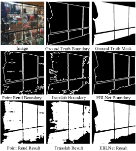
Figure 1: Illustration of glass-like object segmentation. Row one gives the input image and ground truth. Row two shows the comparison results on the boundary. Row three compares the final segmentation results. Our method (EBLNet) works the best among them [26, 65].

Glass-like objects widely exist in the real world: bottles, windows, and mirrors are made of glass. They are mostly transparent, often amorphous solid. Sensing these objects is useful for many applications. For example, robots need to avoid fragile objects (e.g., glasses, vases, and mirrors) during their navigation. These objects differ from others in that: (1) they do not have a fixed pattern, their shape often vary, (2) because of their transparent nature, they are mostly confounded with the surrounding background, the appearance of their inner region varying according to the scene, (3) not all glass regions are salient, sometimes there are some occlusions or reflections on it. These problems make such glass-like object segmentation a difficult task. Current state-of-the-art semantic segmentation models [77, 8, 14] and salient object detection methods [38, 74] are significantly challenged. Similarly, though previous works on boundary detection [66, 72, 12] achieve remarkable results on traditional benchmarks [54, 1], they can not work well on glass-like object scenarios due to the confounding appearance of the object’s inner and outer parts. Fig. 1 illustrates a complex example for glass segmentation.

To address the above issues, the very first step is to construct large-scale datasets [44, 68, 65]. From these datasets, the task is cast as a two-class semantic segmentation problem, where glass-like objects are foreground and the rest is background. Based on these newly proposed datasets, state-of-the-art methods of both semantic segmentation [14, 77, 8] and salient object detection [38, 63] obtain unsatisfactory results. For example, DeeplabV3+ (semantic segmentation method) [8] and EGNet (salient object detection method) [78] only get 84.2 and 85.0 mIoU on GDD [44] test set. Very few dedicated methods to solve this challenging task have been introduced so far [44, 65, 68]. GDNet [44] proposes to use multiple well-designed large-field contextual feature integration to enhance the context representation for modeling glass object context. MirrorNet [68] uses a contextual contrasted feature extraction module for mirror detection. In contrast, Translab [65] proposes to use boundary-aware information to improve the segmentation performance. However, the first two [68, 44] bring too much comparison and context information, which is not very helpful. The last one ignores the pixel-wised relationship on the boundary, limiting the generality of learning objects with various shapes.

When humans locate and recognize the glass-like object, one crucial cue is the entire boundary of such object. Instead, comparing the inner object appearance and its surrounding background used in MirrorNet and GDNet cannot help much to segment since they are mainly confounded.

To reduce the influence of complex inner parts and get accurate boundary prediction, motivated by differential edge detection and morphological processing [13, 47], we propose a novel and efficient module named Refined Differential Module (RDM). RDM works in a coarse-to-fine manner with residual learning. Specifically, rather than simply predict the edge of objects with edge supervision, we also supervise the non-edge part following the same spirit of dilation operation in morphological processing [52] to eliminate noise brought by the inner part and background. This process helps generate smoother non-edge features. Then the thinner and more accurate edge features can be generated by subtracting the non-edge features from the whole features. In order to use the precise edge prediction to enhance global feature learning around the edge then improve the final prediction, we further propose an efficient edge-aware Point-based Graph convolution network Module (PGM). In network design, our modules can be plugged into many semantic segmentation methods. Take DeeplabV3+ [8] as an example, our modules can be inserted behind the ASPP module. Finally, we propose a joint loss function to simultaneously supervise the edge part, non-edge part, and final segmentation result.

Quantitatively, our approach achieves a significant gain in performance w.r.t. previous work [26, 65] (around 3%-5% in mIoU), on three recent proposed glass-like object segmentation datasets (Trans10k [65], GDD [44], and MSD [68]), and hence achieves new state-of-the-art results. Visually, our method detects more accurate boundaries, resulting in a more precise segmentation result (see Fig. 1). This backs our original motivation that finer boundary prediction leads to more refined segmentation.

We further verify the generalization performance of our model in Sec. 4.4 via two different setting, one of them carries out the experiments on another three general segmentation datasets, including CityScapes [11], BDD [70], and COCO Stuff [4].
Our main contributions are three-fold:

• We analyze some existing methods, like DANet [14], Trans10k [65], and GDNet [44] then identify their drawbacks for glass-like object segmentation task.

• We propose a Refined Differential Module (RDM) to generate precise edge and an efficient Point-based Graph convolution network Module (PGM) for global edge feature learning. Then a joint loss function is proposed to supervise the whole model.

• Extensive experiments and analyses indicate the effectiveness and generalization of our model. We achieve the state-of-the-art results on three challenging recent proposed glass-like object segmentation benchmarks.

2 Related Work

Glass-like Object Segmentation: Glass object segmentation comprises two sub-tasks, sometimes processed in a distinct way: mirror segmentation and transparent object segmentation. Giver a single RGB image, mirror segmentation aims to segment mirror regions. In [68], the author proposes a large benchmark for this topic. They attempt to use contextual contrasted features in a segmentation scheme. However, contrasted features may not help for transparent object segmentation since semantic and low-level discontinuities in mirrors may not happen for transparent objects. Transparent object segmentation aims to segment transparent objects from a single RGB image. In  [23], the author uses a polarization camera to capture multi-modal imagery to enhance the transparent object segmentation. Authors of both  [44] and  [65] propose a new benchmark for this task.  [65] proposes Translab to encode the boundary information while  [44] integrates abundant contextual cues. Both of them have failed to explore the relationship between edge features and non-edge features, which is well-considered in our method.

Boundary Processing: Boundary processing is a classical computer vision problem. In the era of deep learning, some CNN-based methods have significantly pushed the development of this field, such as [66, 43, 28, 12]. Several works have been proposed to obtain satisfactory boundary localization with structure modeling, such as boundary neural fields [2], affinity field [24] and random walk [3]. Recently, PointRend [26] is proposed to refine the coarse masks by rending some points on them through one shared multi-layer perception module. Some works [10, 32, 16] fuse the learned edge map into segmentation head to improve segmentation performance on the boundary, while GSCNN [55] uses a gated layer to control the information flow between edge part and regular part. All these works focus on locally mining the edge information and ignore the global shape information, which is essential for recognizing the glass-like objects. Our PGM uses global edge features to improve the segmentation results of glass-like objects.

Semantic Segmentation: Recent methods for semantic segmentation are predominantly based on FCNs [42, 64, 33, 31]. Several works [37, 80] use some structured prediction modules like conditional random fields [29] (dense CRFs) to refine outputs. Current state-of-the-art methods [77, 7, 14] improve the segmentation performance by designing specific heads with dilated convolutions [71] to capture contextual information. Recently, non-local operators [58, 14, 20, 75] based on the self-attention mechanism [56] are used to harvest pixel-wise context from the whole image. Similarly, graph convolution networks [35] propagate information over the entire image by reasoning in the interaction space. Although these methods achieve state-of-the-art results on standard benchmarks such as Cityscape [11], ADE [81], BDD [70], and COCO Stuff [4], their performance on glass-like object segmentation benchmarks will drop a lot due to noise of background context that are introduced by the non-local operators. Our method focuses more on the edges and avoids introducing too much background information.

Salient Object Detection: Glass-like object segmentation can be viewed as one specific case of salient object detection. Many state-of-the-art methods [74, 40, 78, 46, 79, 15] are devoted to fully utilize the integration of multi-level features to enhance network performance. Recent works [41, 9] apply attention mechanisms to learn both global and local context or adopt foreground/background attention maps to help detect salient objects and eliminate non-salient objects. Our work also utilizes the multi-scale feature representation by designing a cascade differential refined model for better location cues to get fine-grained masks.

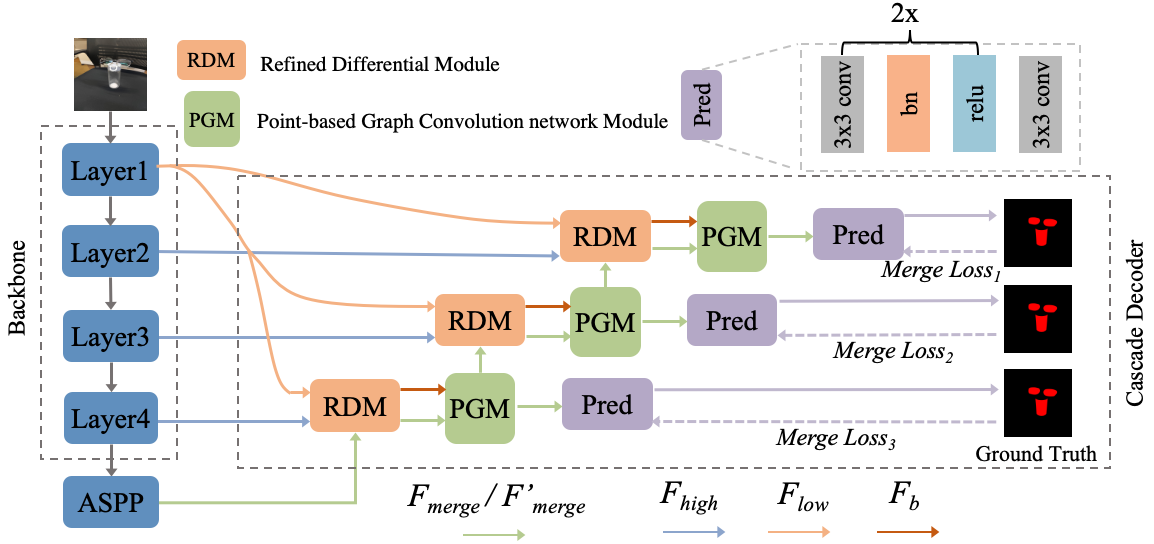
Figure 2: Cascade Network Architecture. We adopt DeeplabV3+ as baseline for illustration where the RDM and PGM are connected in a cascaded order. Best view it on screen and zoom in.

3 Method

3.1 Overview

Our framework utilizes and combines the different levels of feature maps (high-level for semantic, low-level for edge-like features) obtained from a pre-trained backbone network. Our observation has two-fold: (1) edge information (from low-level feature maps) are necessary to ‘reinforce’ semantic region cues (obtained from high-level maps), (2) precise and robust delineation of boundaries enables a fine and accurate segmentation result. These observations lead us to design two modules: a Refined Differential Module (RDM) and an edge-aware Point-based Graph convolution network Model (PGM). RDM (Sec. 3.2) outputs the precise edges of the glass-like objects and the initial segmentation features. PGM (Sec. 3.3) learns to refine the initial segmentation features using the precise boundary generated by the RDM, it appears in coupling with the RDM. In Sec. 3.4, RDM and PGM are integrated into a cascaded architecture network. The whole model is supervised in three fashions: boundaries-wise, residual-wise (nonboundary-wise), and merge-wise (segmentation-wise) via a joint loss function. Fig. 2 illustrates the overall framework.

Note that, though Translab [65] also uses edge to improve the segmentation results, it has two main drawbacks: (1) directly predict the edge cannot avoid noises from glass objects’ inner part, leading to undiscriminating edge feature and inaccurate edge prediction, (2) the direct usage of inaccurate edge prediction to improve segmentation feature will lead to some false guidance. Our two modules work in complementary ways to deal with these problems.

3.2 Refined Differential Module

Overview: The structure of RDM is shown in Fig. 3(a), inputs of the RDM are $F_{low},F_{high}$ and $F_{in}$, which are low-level features of backbone, relative high-level features of backbone, and outputs of other modules (such as ASPP module in DeeplabV3+ [8]), respectively. Compared with $F_{high}$, $F_{in}$ has a larger receptive field and is smoother. With these three inputs, RDM aims to learn: (i) precise edge prediction, $F_{b}$, (ii) ‘residual’ feature maps, $F_{residual}$ (segmentation features except the edge region), (iii) ‘complete’ segmentation feature maps, $F_{merge}$, (that characterizes both residual region and edge region), which serves as the input of the next module. Supervision is applied for each feature type. Since there are two refinements and one subtraction (which will be explained later) of our module, we name it Refined Differential Module or RDM for short.

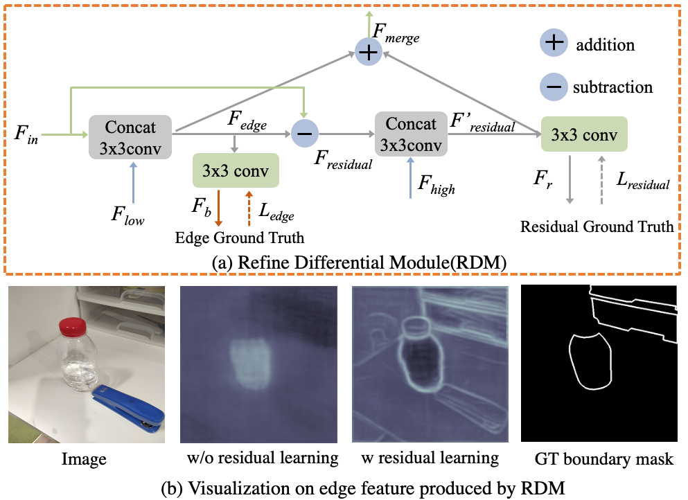
Figure 3: (a) Refined Differential Module, $L_{edge}$ and $L_{residual}$ are losses of edge part prediction and residual part prediction. (b) Feature visualization comparison. The second and the third column represent the edge feature $F_{edge}$ before and after using residual learning. Best view it on screen and zoom in.

Coarse edge prediction: This step generates the edge prediction $F_{b}$ and non-edge features $F_{residual}$ . Since low-level features $F_{low}$ can provide detailed positional cues for edge prediction proven in previous works [8, 26], we first refine the input feature $F_{in}$ with low-level features $F_{low}$ (after bi-linearly resizing the feature maps) by first concat them. Then, a convolution operator is used to get the refined input feature, $F_{edge}\in\mathbb{R}^{H\times W\times C}$, this process can be formulated by Equ. 1.

$$F_{edge}=g_{3\times 3}([F_{low};F_{in}])$$ (1)

where $[;]$ and $g_{n\times n}$ denote concatenation and convolution, respectively. Additionally, we compute the residual (i.e. non-edge) feature $F_{residual}$ by subtracting $F_{edge}$ from $F_{in}$, i.e. the difference between the coarse edge map $F_{edge}$ and the input features $F_{in}$. This procedure can be formulated as Equ. 2:

$$F_{residual}=F_{in}-F_{edge},$$ (2)

We further transform $F_{edge}$ to the edge prediction $F_{b}\in\mathbb{R}^{H\times W\times 1}$ (via a 2-layer convolution), which is supervised using a ground-truth edge map.

Fine-grained Edge Prediction with Residual Learning: Our motivation has two-fold: (1) For the glass-like objects, the residual part may bring noises for edge prediction. Better feature representation of the residual part will make it easier to learn a better edge around the glass object. (2) Since $F_{edge}$ of the first step may not be very accurate, Equ. 2 may remove some vital features for $F_{residual}$. So we adopt another fine-grained feature $F_{high}$ generated from the backbone to refine $F_{residual}$ and get $F^{\prime}_{residual}$ for better residual learning. This process is formulated by Equ. 3.

$$F^{\prime}_{residual}=g_{3\times 3}([F_{residual};F_{high}])$$ (3)

The prediction $F_{r}$ of the residual part is generated using another two $3\times 3$ convolution layers, as shown in Equ. 4

$$F_{r}=g_{3_{\times}3}\circ g_{3\times 3}(F^{\prime}_{residual})$$ (4)

$F_{r}$ is supervised using a ground truth residual mask. This indirect supervision of $F^{\prime}_{residual}$ forces it to be smooth, thus contributing to accurate $F_{b}$. The convolution operation here performs a similar role as the dilation operation in morphological processing [47] (i.e. making inner part ‘grow up’ towards borders). Finally, we have $F_{merge}=F^{\prime}_{residual}+F_{edge}$. If there is no PGM connected to RDM, $F_{merge}$ is used to generate the prediction $F_{m}$ using a segmentation head consisting of three convolutional layers, two batch normalization layers [21], and two non-linear activation function, shown in Fig. 2 (the purple module: Pred).

To best show the effect of our module, we give the feature visualization on $F_{edge}$ for both coarse edge prediction and fine-grained edge prediction with residual learning in Fig. 3(b). We use Principal component analysis (PCA) [60] to reduce the dimension of $F_{edge}$ into three dimensions for visualization. Compared to only supervising the edge part, joint supervision on both edge and residual part can produce more discriminative edge features, which supports our motivation for edge sharpening via residual learning.

3.3 Edge-aware Point-based GCN Module

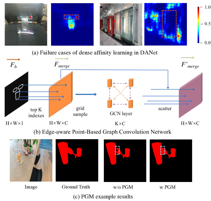
Figure 4: Subfigure (a) shows two failure cases for dense affinity learning in DANet [14], selected points are marked red. The second and the fourth images show the affinity map of selected points. For the first image, the red point is on the glass, while its affinity map mainly comes from the bottle not the glass. For the third image, the affinity map of the red point does not come from the glass to which it belongs. (b) describes the pipeline of PGM. (c) proves the effectiveness of PGM. After using PGM, the boundary is much smoother and more consistent. Best view it on screen.

In order to enforce finer boundary delineation on $F_{merge}$, we further propose an efficient Point-based Graph convolution network (GCN) Module. The key idea is to exploit the accurate edge prediction $F_{b}$ to refine the feature map $F_{merge}$ at the boundary points. To do so, our module accounts for the spatial correlation between edge points. We coin this module Point-based GCN Module (PGM).

Recall on Graph Convolution Network: Graph convolution [25] is a highly efficient and differentiable module that allows long-range interaction in a single operation. Given a graph $\mathbb{G}=\{\mathbb{E},\mathbb{V}\}$ where are $\mathbb{V}$ the nodes and $\mathbb{E}$ the pairwise links between nodes, the graph convolution operation can be defined as [25] with Equ. 5 :

$$\tilde{\mathbf{X}}=\sigma(\mathbf{W}\mathbf{X}\mathbf{A})$$ (5)

with $\sigma(\cdot)$ a non-linear activation function, $\mathbf{A}\in\mathbb{R}^{N\times N}$ is the adjacency matrix characterising the neighbourhood relations of the graph, $\mathbf{W}\in\mathbb{R}^{D\times\tilde{D}}$ is a weight matrix and $\mathbf{X}$ is a $D\times N$ matrices characterizing the $N$ nodes in a $D$ dimensional space. However, directly applying GCN as dense affinity graph [14, 34] for glass-like object segmentation task is a trivial solution since the huge appearance variation on the surface of glass objects. As shown in Fig. 4(a), with the dense affinity graph, inner parts can not provide the context cues to support the final prediction on the visualized affinity maps. Thus we apply GCN only on point-wised boundary features of $F_{merge}$ to enhance its representation.

Point-based Graph Convolution Network on edge: The pipeline of PGM is shown in Fig. 4(b). Given edge prediction $F_{b}$ and segmentation feature $F_{merge}$, we sample the nodes $V$ from $F_{b}$ according to their confidence score and give them attributes to $F_{merge}$. Specifically, we first select at most $K$ points with the highest confidence in $F_{b}$. Then, we use the indices of these points to sample the corresponding $K$ point features from $F_{merge}$. This allows us to build the feature matrix $\mathbf{G}_{in}\in\mathbb{R}^{C\times K}$, where $C$ is the number of channels of $F_{merge}$. Assuming a fully connected graph (all $K$ points are connected), the graph convolution operation can be performed as a fully connected layer. Then the adjacency matrix $\mathbf{A}_{g}$ is simply a $1\times 1$ convolutional layer that can be learned in a standard back-propagated way. Then we can write the output features with Equ. 6 :

$$\mathbf{G}_{out}=\sigma\left(\mathbf{W}_{g}\mathbf{G}_{in}\mathbf{A}_{g}\right)$$ (6)

with $\mathbf{A}_{g}\in\mathbb{R}^{K\times K}$. $\mathbf{W}_{g}\in\mathbb{R}^{C\times C}$ is a feature projection matrice learned along with $\mathbf{A}$. After applying one layer of graph convolution and obtaining $\mathbf{G}_{out}$, we place back the point features of $G_{out}$ into $F_{merge}$ according to their indices and get the refined segmentation features $F^{\prime}_{merge}$, which is used to generate the $F_{m}$ using the aforementioned Pred.

PGM is efficient and effective in handling glass-like transparent objects since the global edge information is essential to recognize a glass-like object. As shown in Fig. 4(c), after PGM, the final segmentation boundary is smoother and more consistent.

3.4 Network Architecture and Loss function

Cascade Refined Decoder: Cascade refinement has been proven effective for various tasks [5, 36]. We also design a cascade decoder. For each layer, there are three modules (RDM, PGM, Pred) connected serially. The outputs of RDM are $F_{b}$ and $F_{merge}$. Then PDM utilizes $F_{b}$ to improve the boundary part’s feature of $F_{merge}$ and gets $F^{\prime}_{merge}$. Finally, $F^{\prime}_{merge}$ is used to generate the segmentation prediction $F_{m}$ via Pred. If it is not the last stage, we take the output of PGM $F^{\prime}_{merge}$ as the new input $F_{in}$ for the next stage’s RDM. The $F_{high}$ is designed by introducing different stages’ features of the backbone network. We use the $F_{m}$ of the last cascade layer as the final output. Since our proposed modules are lightweight, cascade learning does not lead to much computation cost during the inference while contributes to a significant gain on final results.

Network Architecture: Fig. 2 illustrates the whole network architecture, which bases on the state-of-the-art semantic segmentation model DeeplabV3+ [8]. Here we utilize dilated ResNet as backbone [17, 71] only for illustration purpose. The output stride of backbone is 8 in our experiments unless otherwise specified. The cascade decoder is inserted after the ASPP module [8], the output feature of ASPP module is served as the input feature $F_{in}$ in the first stage. Our method can be easily added to other methods [42, 77, 14] which can be found in the experiment part.

Loss function Design: There are three different prediction results at each cascade stage, namely $F_{b}$, $F_{r}$, $F_{m}$, which are predictions of edge part, residual part and merge part, respectively. We define a joint loss function to supervise them simultaneously shown in Equ. 7.

$$L_{joint}= \lambda_{1}L_{residual}(F_{r},G_{r})+\lambda_{2}L_{edge}(F_{b},G_{e})+$$ (7)

$$\lambda_{3}L_{merge}(F_{m},G_{m})$$

$G_{m}$ represents the original ground truth, the ground truth of edge part $G_{e}$ generated from $G_{m}$ is a binary edge mask with thickness 8. When generating the ground truth of residual part $G_{r}$ the corresponding position of the positive pixel of $G_{e}$ in $G_{r}$ is marked as ignore and the other pixels of $G_{r}$ are the same as $G_{m}$. $\lambda_{1}$, $\lambda_{2}$ and $\lambda_{3}$ are used to balance the importance among $L_{residual},L_{edge}$, $L_{merge}$. In our experiments, $\lambda_{1}=1,\lambda_{2}=3,\lambda_{3}=1$. $L_{merge}$ and $L_{residual}$ are standard Cross-Entropy Loss. $L_{edge}$ is Dice Loss [45]. The final loss function is an addition of each stage, formulated as $L=\sum_{n=1}^{N}L_{joint}^{n}$, where $N$ represents the number of cascade layer. Besides, in the PGM, we only use the indices of the selected edge points then the sample and place back operations can be implemented easily by some deep learning framework (like grid sample and scatter in PyTorch [48]). Thus, the overall model is end-to-end trainable.

4 Experiment

Baseline	+RDM	+cascade	+PGM	mIoU $\uparrow$	mBER $\downarrow$	mAE $\downarrow$
Deeplabv3+	-	-	-	85.4	6.73	0.075
	✓	-	-	89.2	4.63	0.054
	✓	✓	-	90.1	4.15	0.049
	✓	✓	✓	90.7	3.97	0.047

(a) Effect of each component.

$L_{merge}$	$L_{edge-bce}$	$L_{edge-dice}$	$L_{residual}$	mIoU $\uparrow$	mBER $\downarrow$	mAE $\downarrow$
✓	-	-	-	88.3	5.02	0.060
✓	✓	-		89.4	4.48	0.053
✓	✓	-	✓	90.4	4.12	0.049
✓	-	✓	✓	90.7	3.97	0.047

(b) Effect of loss function design.

Settings	mIoU $\uparrow$	mBER $\downarrow$	mAE $\downarrow$
All operators	89.2	4.63	0.054
w/o $F_{low}$	88.8	4.92	0.059
w/o $F_{high}$	88.4	5.01	0.058
w/o Both	88.2	4.98	0.058
w/o residual learning	86.4	6.17	0.070

(c) Effect of each component in RDM.

Method	mIoU $\uparrow$	F1(12px) $\uparrow$	F(9px) $\uparrow$	F1(5px) $\uparrow$	F1(3px) $\uparrow$
baseline	85.4	77.6	73.5	66.6	56.7
+RDM	89.2	84.7	81.6	77.6	68.5
+RDM & PGM	89.5	85.8	83.1	79.2	73.3

(d) Effectiveness on boundary refinement.

Network	mIoU $\uparrow$	mBER $\downarrow$	mAE$\downarrow$
FCN	83.2	7.94	0.094
+our modules	87.9	5.04	0.062
PSPNet [77]	83.5	8.34	0.089
+our modules	88.6	4.93	0.058
DANet [14]	84.1	7.03	0.084
+our modules	87.8	5.14	0.062

(e) Application on Other Architectures.

Table 1: Ablation studies. We first verify the effect of each module and loss function in (a) and (b) in terms of mIoU, mBER and mAE. Then we give a detailed component analysis in RDM in (c), and use boundary metrics to verify each module’s effect in (d). Finally, verify the various architectures in (e) to show the generality of our proposed modules. All the results are reported on the validation set of Trans10k. Best view it on screen and zoom in.

4.1 Datasets and evaluation metrics

Datasets: (a) Trans10k [65] dataset contains 10,428 images with two categories of transparent objects, including things and stuff. For this dataset, 5000, 1000, and 4428 images are used for train, validation, and test, respectively. (b) GDD [44] is another large-scale glass object segmentation dataset covering diverse daily-life scenes (such as office, street). For dataset split, 2980 images are randomly selected for training and the remaining 936 images are used for testing. (c) MSD [68] is a large-scale mirror dataset. For dataset split, 3063 images are used for training while 955 images are used for testing. We use the Trans10k for ablation studies and analyses and also report results on the GDD and MSD.

Evaluation metrics: Following the previous work [65, 44, 68] , for the Trans10k dataset, we adopt four metrics for quantitatively evaluating the model performance unless otherwise specified. Specifically, we use the (mean) intersection over union (IoU/mIoU) and pixel accuracy (ACC) metrics from the semantic segmentation field. Mean absolute error (mAE) from the salient object detection field is also used. On top of that, we use the balance error rate (BER/mBER), which considers the unbalanced areas of transparent (mirror) and non-transparent (non-mirror) regions. Following [44, 68], F-measure is also used to evaluate the model performance of GDD and MSD datasets. When evaluating the accuracy of predicted boundaries, following [55], we use F1-score as the metric.

4.2 Experiment on Trans10k

Overview: We firstly perform ablation studies on the validation set. Then visualization analysis is given to show the accurate segmentation results. Finally, we compare our model with the state-of-the-art models on the test set.

Trans10k implementation details: We adopt the same training setting as the original Trans10k [65] paper for fair comparison. The input images are resized to the resolution of 512$\times$512. We use the pre-trained ResNet50 as the backbone and refine it along with other modules. We use 8 GPUs for all experiments and batch size is set to 4 per GPU. The learning rate is initialized to 0.01 and decayed by the poly strategy with the power of 0.9 for 16 epochs. We report mIoU, mBER, mAE in ablation study and also report ACC when comparing with other methods on test set.

Ablation on Each Components: We first verify the effectiveness of each module with DeeplabV3+ [8] as the baseline in Tab. 1(a). After using the proposed RDM, there exists a significant gain over the baseline by 3.8% mIoU, 2.1 in mBER and 0.021 in mAE. These results indicate the importance of precise boundaries generation for glass object segmentation. After appending more RDM modules in the cascade framework, the performance further gains 0.9% mIoU. Finally, based on the precise boundary, applying our proposed PGM, our method gain another 0.6% mIoU on the cascade model. Although PGM does not provide as much numerical improvement as RDM because of the small number of pixels at the boundaries, it does provide a significant visual improvement, as shown in Fig. 4(c).

Ablation on Loss function design: Then we explore the impact of loss function by fixing each component where the number of sampled points is set to 96 in PGM, and the number of cascade stages is set to 3. Results are shown in Tab. 1(b), after using binary Cross-Entropy loss ($L_{edge-bce}$) as $L_{edge}$, we find 1.1% mIoU gain. With an additional $L_{residual}$, we find another 1.0% mIoU gain which indicates that dual supervision is conducive to sharpen edge generation then improve the final prediction. Compared to using binary Cross-Entropy loss as $L_{edge}$, Dice loss ($L_{edge-dice}$) leads to 0.3% mIoU gain since dice loss can better handle the imbalance problems for foreground objects.

Ablation on RDM: We give detailed ablation studies on each component in RDM by removing it from the complete RDM in Tab. 1(c). We set the cascade number to 1 and do not use PGM. Removing $F_{low}$ or $F_{high}$ in the first step or the second step of RDM results in mIoU decline of 0.4% and 0.8%, respectively. Removing both of them results in mIoU degradation of 1.0%. After removing the subtraction operation and residual learning, there is a clear drop on all metrics indicating the importance of boundary sharpening.

Ablation on boundary refinement: We present a detailed comparison on boundary using F1-score [55] with four different thresholds in Tab. 1(d) where the cascade is not used. For each threshold, results obtain significant gains after using RDM. The gain becomes more significant when the neighbor pixels decrease (from 12 pixels to 3 pixels). These results indicate that our method can generate a precise boundary. The improvement of mIoU also proves our motivation that better boundary prediction is beneficial to produce better segmentation results. After using PGM, there are more gains in all the metrics in this strong baseline.

Application on more segmentation methods: In addition to DeeplabV3+, we carry on experiments on various other network architectures including, FCN [42], PSPNet [77] and DANet [14]. Our modules are appended at the end of the head of these networks, and are trained with the same setting as DeeplabV3+. As shown in Tab. 1(e), our modules improve those methods by a large margin, which proves the generality and effectiveness of our modules.

Comparison with the state-of-the-arts: Following [65], we report mIoU, Acc, mAE, mBER on Trans10k test set. As shown in Tab. 2, our method achieves the state-of-the-art results on four metrics with output stride 16 for fair comparison with Translab [65]. After changing the output stride to 8 in the backbone, our method obtains a better result.

Method	mIoU $\uparrow$	Acc$\uparrow$	mAE $\downarrow$	mBER$\downarrow$
Deeplabv3+ (MobileNetv2) [8]	75.27	80.92	0.130	12.49
HRNet [57]	74.56	75.82	0.134	13.52
BiSeNet [69]	73.93	77.92	0.140	13.96
DenseAspp [67]	78.11	81.22	0.114	12.19
Deeplabv3+ (ResNet50) [8]	84.54	89.54	0.081	7.78
FCN [42]	79.67	83.79	0.108	10.33
RefineNet [36]	66.03	57.97	0.180	22.22
Deeplabv3+ (Xception65) [8]	84.26	89.18	0.082	8.00
PSPNet [77]	82.38	86.25	0.093	9.72
Translab (ResNet50) [65]	87.63	92.69	0.063	5.46
EBLNet (ResNet50, OS16)	89.58	93.95	0.052	4.60
EBLNet (ResNet50, OS8)	90.28	94.71	0.048	4.14

Table 2: Comparison to state-of-the-art on Trans10k test set. All methods are trained on Trans10k training set under the same setting and all models use single scale inference. OS means the output stride in the backbone.

4.3 Experiment on GDD and MSD

Experiment on GDD: We adopt the same setting as the original paper [44] for fair comparison where the input images are resized into $416\times 416$ and are augmented by horizontally random flipping. The total training epoch is 200. The learning rate is initialized to 0.003 and decayed by the poly strategy with the power of 0.9. We also give results with different backbones for better comparison. As shown in Tab. 3, our method achieves the state-of-the-art result on this dataset on five different metrics without using conditional random fields (CRF) [29] as the post-processing.

Method	IoU $\uparrow$	Acc$\uparrow$	$F_{\beta}\uparrow$	mAE$\downarrow$	BER$\downarrow$
PSPNet [77]	84.06	0.916	0.906	0.084	8.79
DenseASPP [67]	83.68	0.919	0.911	0.081	8.66
DANet [14]	84.15	0.911	0.901	0.089	8.96
CCnet [20]	84.29	0.915	0.904	0.085	8.63
PointRend [27]	86.51	0.933	0.928	0.067	6.50
DSS [18]	80.24	0.898	0.890	0.123	9.73
PiCANet [41]	83.73	0.916	0.909	0.093	8.26
BASNet [51]	82.88	0.907	0.896	0.094	8.70
EGNet [78]	85.04	0.920	0.916	0.083	7.43
DSC [19]	83.56	0.914	0.911	0.090	7.97
BDRAR [82] †	80.01	0.902	0.908	0.098	9.87
MirrorNet [68] (ResNext101) †	85.07	0.918	0.903	0.083	7.67
GDNet [44] (ResNext101)	87.63	0.939	0.937	0.063	5.62
EBLNet (ResNet101)	88.16	0.941	0.939	0.059	5.58
EBLNet ((ResNext101)	88.72	0.944	0.940	0.055	5.36

• †CRF is used for post-processing.

Table 3: Comparison to state-of-the-art on GDD test set. All methods are trained on GDD training set under the same setting and all models use single scale inference.

Method	CRF	IoU $\uparrow$	Acc$\uparrow$	$F_{\beta}\uparrow$	mAE$\downarrow$	BER$\downarrow$
PSPNet [77]	-	63.21	0.750	0.746	0.117	15.82
ICNet [76]	-	57.25	0.694	0.710	0.124	18.75
PointRend [27] (Deeplabv3+)	-	78.81	0.936	0.872	0.054	8.95
DSS [18]	-	59.11	0.665	0.743	0.125	18.81
PiCANet [41]	-	71.78	0.845	0.808	0.088	10.99
RAS [9]	-	60.48	0.695	0.758	0.111	17.60
DSC [19]	-	69.71	0.816	0.812	0.087	11.77
BDRAR [82]	$\surd$	67.43	0.821	0.792	0.093	12.41
MirrorNet (ResNeXt101) [68]	$\surd$	78.95	0.935	0.857	0.065	6.39
EBLNet (ResNet101)	-	78.84	0.946	0.873	0.054	8.84
EBLNet (ResNext101)	-	80.33	0.951	0.883	0.049	8.63

Table 4: Comparison to state-of-the-art on MSD test set. All methods are trained on the MSD training set. All models use single-scale inference.

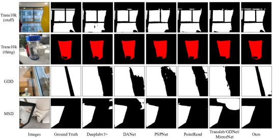
Figure 5: Visualization and comparison results on Three glass-like object segmentation datasets. The 1st and 2nd row of the 7th column are results of Translab [65], the 3rd row of the 7th column is a result of GDNet [44], the 4th row of the 7th column is a result of Mirrornet [68]. Compared with other methods, our method has much better results.

Experiment on MSD: Following the setting in MirrorNet [68], input images are resized to a resolution of 384 $\times$ 384 and are augmented by horizontally random flipping. The learning rate is initialized to 0.002 and decayed by the poly strategy with the power of 0.9. We train our model for 160 epochs. As shown in Tab. 4, our method achieves state-of-the-art results in four different metrics.

Visual Results Comparison: Fig. 5 gives the some visual results on all the three datasets. Our method can obtain superior segmentation results compared with other methods and has fine-grained boundary results on mirrors or glass. More results can be found in the supplemental file.

Method	Parameters $\downarrow$	Inference Time $\downarrow$	mIoU $\uparrow$	BER $\downarrow$	mAE $\downarrow$
MirrorNet [68]	103.3M	37ms	81.3	8.98	0.094
GDNet [44]	183.2M	41ms	82.6	8.42	0.088
Translab [65]	65.2M	26ms	85.1	7.43	0.081
EBLNet	46.2M	24ms	86.0	6.90	0.074

Table 5: Comparison results with related methods on GDD test set. The speeds are tested with $416\times 416$ inputs. For fair comparison, all models’ backbone are ResNet50 and all the inference times are tested with one V100 GPU.

Efficiency and Effectiveness: To further show the efficiency and effectiveness of our model on glass-like object segmentation, we compare parameters and inference time of our network with recent proposed glass-like object segmentation networks, including MirrorNet [68], GDNet [44] and Translab [65] on GDD test set. Results are shown in Tab. 5. Our method has the fewest parameters and fastest inference speed. Our method also achieves the best precision.

4.4 Generalization Experiments

In this section, we prove the generality of our method via two different experiment settings: (1) training our model on one glass-like object segmentation dataset then fine-tune on another glass-like object segmentation dataset, (2) evaluating our model on other three general segmentation datasets, including Cityscapes [11], BDD [70] and COCO Stuff [4]. Training settings can be found in the supplemental file.

OD	FTD	mIoU	SFT mIoU	OD	FTD	mIoU	SFT mIoU
Trans10k	MSD	78.43	78.84	MSD	Trans10k	86.42	90.28
Trans10k	GDD	87.94	88.16	GDD	Trans10k	89.01	90.28
MSD	GDD	87.07	88.16	GDD	MSD	79.41	78.84

Table 6: OD: original dataset. FTD: fine-tune dataset. Models are pre-trained on OD then fine-tuned on FTD and report mIoU on the test set of FTD. FTD mIoU: when model is trained from scratch on the FTD, the mIoU on the FTD test set. The mIoUs are very close to SFT mIoUs. Note that, the mIoU even surpass SFT mIoU when OD is GDD and FTD is MSD. Backbones are ResNet101.

Method	dataset	mIoU $\uparrow$	F1(12px) $\uparrow$	F1(9px) $\uparrow$	F1(5px) $\uparrow$	F1(3px) $\uparrow$
Deeplabv3+ [8]	Cityscapes	77.4	78.9	77.5	73.9	62.3
+PointRend [77]	Cityscapes	78.3	79.5	78.5	74.3	63.6
+ours	Cityscapes	79.1	81.4	80.1	76.5	67.0
Deeplabv3+ [8]	BDD	60.8	76.4	75.2	70.6	61.5
+PointRend [77]	BDD	61.2	78.4	77.2	72.3	63.6
+ours	BDD	63.1	80.6	79.4	75.4	66.4
Deeplabv3+ [8]	COCO Stuff	33.6	73.3	71.8	70.6	66.7
+PointRend [77]	COCO Stuff	34.1	73.8	72.3	71.1	67.4
+ours	COCO Stuff	34.7	74.9	72.9	71.5	67.7

Table 7: Comparison results on Cityscapes, BDD and COCO Stuff datasets with DeeplabV3+ and PointRend where X-px means X pixels along the boundaries. All the models are trained and tested with the same setting. Backbones are ResNet50.

Fine-tune Setting: In this setting, we only fine-tune the models for few epochs in the new datasets (2, 10, 8 epochs for Trans10k, GDD and MSD, respectively). Results are shown in Tab. 6, which indicates our method is not overfitted to one specific glass-like object segmentation dataset.

General Segmentation Dataset Setting: In this setting, we use the DeeplabV3+ as the baseline method. Results are shown in Tab. 7. For all the three datasets, both mIoU and F1 scores of our method are better than those of DeeplabV3+ and PointRend. Thus, our method is not overfitted to glass-like object segmentation dataset.

5 Conclusion

In this paper, we focus on solving the glass-like object segmentation problem by enhancing the boundary learning for existing semantic segmentation methods. We propose a novel Refined Differential Module for edge prediction and an efficient edge-aware Point-wised Graph convolution network Module to model global shape representation of glass objects and guide the final prediction. We achieve the new state-of-the-art results on three recent glass-like object segmentation datasets, including Trans10k, MSD, and GDD. Further experiments on three general segmentation datasets, including Cityscapes, BDD, and COCO Stuff prove the generality and superiority of our method.

6 Acknowledgement

This research was supported by the National Key Research and Development Program of China under Grant No. 2018AAA0100400, No. 2020YFB2103402, and the National Natural Science Foundation of China under Grants 62071466, 62076242, and 61976208.

References

- [1] Pablo Arbelaez, Michael Maire, Charless Fowlkes, and Jitendra Malik. Contour detection and hierarchical image segmentation. TPAMI, 2010.
- [2] Gedas Bertasius, Jianbo Shi, and Lorenzo Torresani. Semantic segmentation with boundary neural fields. In CVPR, 2016.
- [3] Gedas Bertasius, Lorenzo Torresani, Stella X. Yu, and Jianbo Shi. Convolutional random walk networks for semantic image segmentation. In CVPR, 2017.
- [4] Holger Caesar, Jasper Uijlings, and Vittorio Ferrari. Coco-stuff: Thing and stuff classes in context. In CVPR, 2018.
- [5] Zhaowei Cai and Nuno Vasconcelos. Cascade r-cnn: Delving into high quality object detection. In CVPR, 2018.
- [6] Ping Chao, Chao-Yang Kao, Yu-Shan Ruan, Chien-Hsiang Huang, and Youn-Long Lin. Hardnet: A low memory traffic network. In ICCV, pages 3552–3561, 2019.
- [7] Liang-Chieh Chen, George Papandreou, Florian Schroff, and Hartwig Adam. Rethinking atrous convolution for semantic image segmentation. arXiv preprint, 2017.
- [8] Liang-Chieh Chen, Yukun Zhu, George Papandreou, Florian Schroff, and Hartwig Adam. Encoder-decoder with atrous separable convolution for semantic image segmentation. In ECCV, 2018.
- [9] Shuhan Chen, Xiuli Tan, Ben Wang, and Xuelong Hu. Reverse attention for salient object detection. In ECCV, 2018.
- [10] Tianheng Cheng, Xinggang Wang, Lichao Huang, and Wenyu Liu. Boundary-preserving mask r-cnn. In ECCV, 2020.
- [11] Marius Cordts, Mohamed Omran, Sebastian Ramos, Timo Rehfeld, Markus Enzweiler, Rodrigo Benenson, Uwe Franke, Stefan Roth, and Bernt Schiele. The cityscapes dataset for semantic urban scene understanding. In CVPR, 2016.
- [12] Ruoxi Deng, Chunhua Shen, Shengjun Liu, Huibing Wang, and Xinru Liu. Learning to predict crisp boundaries. In ECCV, 2018.
- [13] Adrian N Evans and Xin U Liu. A morphological gradient approach to color edge detection. TIP, 2006.
- [14] Jun Fu, Jing Liu, Haijie Tian, Zhiwei Fang, and Hanqing Lu. Dual attention network for scene segmentation. In CVPR, 2019.
- [15] Shang-Hua Gao, Yong-Qiang Tan, Ming-Ming Cheng, Chengze Lu, Yunpeng Chen, and Shuicheng Yan. Highly efficient salient object detection with 100k parameters. In ECCV, 2020.
- [16] Hao He, Xiangtai Li, Kuiyuan Yang, Guangliang Cheng, Jianping Shi, Yunhai Tong, Zhengjun Zha, and Lubin Weng. Boundarysqueeze: Image segmentation as boundary squeezing. arXiv preprint arXiv:2105.11668, 2021.
- [17] Kaiming He, Xiangyu Zhang, Shaoqing Ren, and Jian Sun. Deep residual learning for image recognition. In CVPR, 2016.
- [18] Qibin Hou, Ming-Ming Cheng, Xiaowei Hu, Ali Borji, Zhuowen Tu, and Philip Torr. Deeply supervised salient object detection with short connections. In CVPR, 2017.
- [19] Xiaowei Hu, Lei Zhu, Chi-Wing Fu, Jing Qin, and Pheng-Ann Heng. Direction-aware spatial context features for shadow detection. In CVPR, 2018.
- [20] Zilong Huang, Xinggang Wang, Lichao Huang, Chang Huang, Yunchao Wei, and Wenyu Liu. Ccnet: Criss-cross attention for semantic segmentation. In ICCV, 2019.
- [21] Sergey Ioffe and Christian Szegedy. Batch normalization: Accelerating deep network training by reducing internal covariate shift. In ICML, 2015.
- [22] Qiangguo Jin, Zhaopeng Meng, Tuan D Pham, Qi Chen, Leyi Wei, and Ran Su. Dunet: A deformable network for retinal vessel segmentation. Knowledge-Based Systems, 178:149–162, 2019.
- [23] Agastya Kalra, Vage Taamazyan, Supreeth Krishna Rao, Kartik Venkataraman, Ramesh Raskar, and Achuta Kadambi. Deep polarization cues for transparent object segmentation. In CVPR, 2020.
- [24] Tsung-Wei Ke, Jyh-Jing Hwang, Ziwei Liu, and Stella X. Yu. Adaptive affinity fields for semantic segmentation. In ECCV, 2018.
- [25] Thomas N Kipf and Max Welling. Semi-supervised classification with graph convolutional networks. In ICLR, 2017.
- [26] Alexander Kirillov, Yuxin Wu, Kaiming He, and Ross Girshick. PointRend: Image segmentation as rendering. In CVPR, 2020.
- [27] Alexander Kirillov, Yuxin Wu, Kaiming He, and Ross Girshick. Pointrend: Image segmentation as rendering. In CVPR, 2020.
- [28] Iasonas Kokkinos. Pushing the boundaries of boundary detection using deep learning. arXiv preprint arXiv:1511.07386, 2015.
- [29] John Lafferty, Andrew McCallum, and Fernando CN Pereira. Conditional random fields: Probabilistic models for segmenting and labeling sequence data. 2001.
- [30] Gen Li, Inyoung Yun, Jonghyun Kim, and Joongkyu Kim. Dabnet: Depth-wise asymmetric bottleneck for real-time semantic segmentation. arXiv preprint arXiv:1907.11357, 2019.
- [31] Xiangtai Li, Zhao Houlong, Han Lei, Tong Yunhai, and Yang Kuiyuan. Gff: Gated fully fusion for semantic segmentation. In AAAI, 2020.
- [32] Xiangtai Li, Xia Li, Li Zhang, Cheng Guangliang, Jianping Shi, Zhouchen Lin, Yunhai Tong, and Shaohua Tan. Improving semantic segmentation via decoupled body and edge supervision. In ECCV, 2020.
- [33] Xiangtai Li, Ansheng You, Zhen Zhu, Houlong Zhao, Maoke Yang, Kuiyuan Yang, Shaohua Tan, and Yunhai Tong. Semantic flow for fast and accurate scene parsing. In ECCV, 2020.
- [34] Xia Li, Zhisheng Zhong, Jianlong Wu, Yibo Yang, Zhouchen Lin, and Hong Liu. Expectation-maximization attention networks for semantic segmentation. In ICCV, 2019.
- [35] Yin Li and Abhinav Gupta. Beyond grids: Learning graph representations for visual recognition. NeurIPS, 2018.
- [36] Guosheng Lin, Anton Milan, Chunhua Shen, and Ian D. Reid. Refinenet: Multi-path refinement networks for high-resolution semantic segmentation. In CVPR, 2017.
- [37] Guosheng Lin, Chunhua Shen, Anton van den Hengel, and Ian Reid. Efficient piecewise training of deep structured models for semantic segmentation. In CVPR, 2016.
- [38] Jiang-Jiang Liu, Qibin Hou, Ming-Ming Cheng, Jiashi Feng, and Jianmin Jiang. A simple pooling-based design for real-time salient object detection. In CVPR, 2019.
- [39] Mengyu Liu and Hujun Yin. Feature pyramid encoding network for real-time semantic segmentation. arXiv preprint arXiv:1909.08599, 2019.
- [40] Nian Liu and Junwei Han. Dhsnet: Deep hierarchical saliency network for salient object detection. In CVPR, 2016.
- [41] Nian Liu, Junwei Han, and Ming Hsuan Yang. Picanet: Learning pixel-wise contextual attention for saliency detection. CVPR, 2017.
- [42] Jonathan Long, Evan Shelhamer, and Trevor Darrell. Fully convolutional networks for semantic segmentation. In CVPR, 2015.
- [43] Kevis-Kokitsi Maninis, Jordi Pont-Tuset, Pablo Arbeláez, and Luc Van Gool. Convolutional oriented boundaries: From image segmentation to high-level tasks. PAMI, 2017.
- [44] Haiyang Mei, Xin Yang, Yang Wang, Yuanyuan Liu, Shengfeng He, Qiang Zhang, Xiaopeng Wei, and Rynson W.H. Lau. Don’t hit me! glass detection in real-world scenes. In CVPR, 2020.
- [45] Fausto Milletari, Nassir Navab, and Seyed-Ahmad Ahmadi. V-net: Fully convolutional neural networks for volumetric medical image segmentation. In 3DV. IEEE, 2016.
- [46] Youwei Pang, Xiaoqi Zhao, Lihe Zhang, and Huchuan Lu. Multi-scale interactive network for salient object detection. In CVPR, 2020.
- [47] Giuseppe Papari and Nicolai Petkov. Edge and line oriented contour detection: State of the art. IMAGE VISION COMPUT, 2011.
- [48] Adam Paszke, Sam Gross, Francisco Massa, Adam Lerer, James Bradbury, Gregory Chanan, Trevor Killeen, Zeming Lin, Natalia Gimelshein, Luca Antiga, et al. Pytorch: An imperative style, high-performance deep learning library. In Advances in neural information processing systems, 2019.
- [49] Rudra PK Poudel, Ujwal Bonde, Stephan Liwicki, and Christopher Zach. Contextnet: Exploring context and detail for semantic segmentation in real-time. arXiv preprint arXiv:1805.04554, 2018.
- [50] Rudra PK Poudel, Stephan Liwicki, and Roberto Cipolla. Fast-scnn: Fast semantic segmentation network. arXiv preprint arXiv:1902.04502, 2019.
- [51] Xuebin Qin, Zichen Zhang, Chenyang Huang, Chao Gao, Masood Dehghan, and Martin Jagersand. Basnet: Boundary-aware salient object detection. In CVPR, 2019.
- [52] Jean-Francois Rivest, Pierre Soille, and Serge Beucher. Morphological gradients. Journal of Electronic Imaging, 1993.
- [53] Olaf Ronneberger, Philipp Fischer, and Thomas Brox. U-net: Convolutional networks for biomedical image segmentation. MICCAI, 2015.
- [54] Nathan Silberman, Derek Hoiem, Pushmeet Kohli, and Rob Fergus. Indoor segmentation and support inference from rgbd images. In ECCV. Springer, 2012.
- [55] Towaki Takikawa, David Acuna, Varun Jampani, and Sanja Fidler. Gated-scnn: Gated shape cnns for semantic segmentation. ICCV, 2019.
- [56] Ashish Vaswani, Noam Shazeer, Niki Parmar, Jakob Uszkoreit, Llion Jones, Aidan N Gomez, Łukasz Kaiser, and Illia Polosukhin. Attention is all you need. In NeurIPS, 2017.
- [57] Jingdong Wang, Ke Sun, Tianheng Cheng, Borui Jiang, Chaorui Deng, Yang Zhao, Dong Liu, Yadong Mu, Mingkui Tan, Xinggang Wang, et al. Deep high-resolution representation learning for visual recognition. PAMI, 2020.
- [58] Xiaolong Wang, Ross Girshick, Abhinav Gupta, and Kaiming He. Non-local neural networks. In CVPR, 2018.
- [59] Yu Wang, Quan Zhou, Jia Liu, Jian Xiong, Guangwei Gao, Xiaofu Wu, and Longin Jan Latecki. Lednet: A lightweight encoder-decoder network for real-time semantic segmentation. In ICIP, pages 1860–1864. IEEE, 2019.
- [60] Svante Wold, Kim Esbensen, and Paul Geladi. Principal component analysis. Chemom. Intell. Lab. Syst., 1987.
- [61] Tianyi Wu, Sheng Tang, Rui Zhang, and Yongdong Zhang. Cgnet: A light-weight context guided network for semantic segmentation. arXiv preprint arXiv:1811.08201, 2018.
- [62] Yuxin Wu, Alexander Kirillov, Francisco Massa, Wan-Yen Lo, and Ross Girshick. Detectron2. https://github.com/facebookresearch/detectron2, 2019.
- [63] Zhe Wu, Li Su, and Qingming Huang. Cascaded partial decoder for fast and accurate salient object detection. In CVPR, 2019.
- [64] Tete Xiao, Yingcheng Liu, Bolei Zhou, Yuning Jiang, and Jian Sun. Unified perceptual parsing for scene understanding. In ECCV, 2018.
- [65] Enze Xie, Wenjia Wang, Wenhai Wang, Mingyu Ding, Chunhua Shen, and Ping Luo. Segmenting transparent objects in the wild. ECCV, 2020.
- [66] Saining Xie and Zhuowen Tu. Holistically-nested edge detection. In ICCV, 2015.
- [67] Maoke Yang, Kun Yu, Chi Zhang, Zhiwei Li, and Kuiyuan Yang. Denseaspp for semantic segmentation in street scenes. In CVPR, 2018.
- [68] Xin Yang, Haiyang Mei, Ke Xu, Xiaopeng Wei, Baocai Yin, and Rynson WH Lau. Where is my mirror? In ICCV, 2019.
- [69] Changqian Yu, Jingbo Wang, Chao Peng, Changxin Gao, Gang Yu, and Nong Sang. Bisenet: Bilateral segmentation network for real-time semantic segmentation. In ECCV, 2018.
- [70] Fisher Yu, Haofeng Chen, Xin Wang, Wenqi Xian, Yingying Chen, Fangchen Liu, Vashisht Madhavan, and Trevor Darrell. Bdd100k: A diverse driving dataset for heterogeneous multitask learning. In CVPR, 2020.
- [71] Fisher Yu and Vladlen Koltun. Multi-scale context aggregation by dilated convolutions. ICLR, 2016.
- [72] Zhiding Yu, Chen Feng, Ming-Yu Liu, and Srikumar Ramalingam. Casenet: Deep category-aware semantic edge detection. In CVPR, 2017.
- [73] Yuhui Yuan and Jingdong Wang. Ocnet: Object context network for scene parsing. arXiv preprint, 2018.
- [74] Lu Zhang, Ju Dai, Huchuan Lu, You He, and Gang Wang. A bi-directional message passing model for salient object detection. In CVPR, 2018.
- [75] Li Zhang, Xiangtai Li, Anurag Arnab, Kuiyuan Yang, Yunhai Tong, and Philip HS Torr. Dual graph convolutional network for semantic segmentation. In BMVC, 2019.
- [76] Hengshuang Zhao, Xiaojuan Qi, Xiaoyong Shen, Jianping Shi, and Jiaya Jia. Icnet for real-time semantic segmentation on high-resolution images. In ECCV, 2018.
- [77] Hengshuang Zhao, Jianping Shi, Xiaojuan Qi, Xiaogang Wang, and Jiaya Jia. Pyramid scene parsing network. In CVPR, 2017.
- [78] Jia-Xing Zhao, Jiang-Jiang Liu, Deng-Ping Fan, Yang Cao, Jufeng Yang, and Ming-Ming Cheng. Egnet: Edge guidance network for salient object detection. In ICCV, 2019.
- [79] Xiaoqi Zhao, Youwei Pang, Lihe Zhang, Huchuan Lu, and Lei Zhang. Suppress and balance: A simple gated network for salient object detection. In ECCV, 2020.
- [80] Shuai Zheng, Sadeep Jayasumana, Bernardino Romera-Paredes, Vibhav Vineet, Zhizhong Su, Dalong Du, Chang Huang, and Philip H. S. Torr. Conditional random fields as recurrent neural networks. In ICCV, 2015.
- [81] Bolei Zhou, Hang Zhao, Xavier Puig, Tete Xiao, Sanja Fidler, Adela Barriuso, and Antonio Torralba. Semantic understanding of scenes through the ade20k dataset. IJCV.
- [82] Lei Zhu, Zijun Deng, Xiaowei Hu, Chi-Wing Fu, Xuemiao Xu, Jing Qin, and Pheng-Ann Heng. Bidirectional feature pyramid network with recurrent attention residual modules for shadow detection. In ECCV, 2018.