A model of interacting Navier-Stokes singularities

Abstract

We introduce a model of interacting singularities of Navier-Stokes, named pinçons . They follow a non-equilibrium dynamics, obtained by the condition that the velocity field around these singularities obeys locally Navier-Stokes equations. This model can be seen as a generalization of the vorton model of NovikovNovikov83 , that was derived for the Euler equations. When immersed in a regular field, the pinçons are further transported and sheared by the regular field, while applying a stress onto the regular field, that becomes dominant at a scale that is smaller than the Kolmogorov length. We apply this model to compute the motion of a pair of pinçons . A pinçon dipole is intrinsically repelling and the pinçons generically run away from each other in the early stage of their interaction. At late time, the dissipation takes over, and the dipole dies over a viscous time scale. In the presence of a stochastic forcing, the dipole tends to orientate itself so that its components are perpendicular to their separation, and it can then follow during a transient time a near out-of-equilibrium state, with forcing balancing dissipation.

In the general case where the pinçons have arbitrary intensity and orientation, we observe three generic dynamics in the early stage: one collapse with infinite dissipation, and two expansion modes, the dipolar anti-aligned runaway and an anisotropic aligned runaway. The collapse of a pair of pinçons follows several characteristics of the reconnection between two vortex rings, including the scaling of the distance between the two components, following Leray Leray34 scaling $\sqrt{t_{c}-t}$.

I Introduction

Snapshots of dissipation or enstrophy in turbulent fluids show us that small scales are intermittent, localized and irregular. Mathematical theorems constrain the degree of irregularity of such structures that are genuine singularities of the incompressible Navier-Stokes provided their spatial $\mathbb{L}^{3}$- norm is unbounded (for a review of various regularity criteria, see Gibbon16 ). On the other hand, dissipation laws of turbulent flows suggest that they may be at most Hölder continuous with $h<1/3$ C94 and of diverging vorticity in the inviscid limit. This observation has motivated several theoretical construction of turbulent Navier-Stokes small scale structures or weak solutions of Euler equations, using singular or quasi-singular entities based e.g. on atomic like structures Hicks1899 , Beltrami flows Constantin88 , Mikado flows Buckmaster18 , spirals Lundgren1982 ; Gilbert93 or vortex filaments chorin1991 .

These constructions have fueled a long-standing analytical framework of turbulence, allowing the modeling of proliferating and numerically greedy small scales by a countable (and hopefully numerically reasonable) number of degrees of freedom, provided by characteristics of the basic entities.

A good example of the possibilities offered by such a singular decomposition is provided by the 3D vorton description of Novikov Novikov83 . In this model, the vorticity field is decomposed into $N$ discretized singularities infinitely localized (via a $\delta$ function) at points $r_{\alpha}$, ($\alpha=1...N$), each characterized by a vector $\boldsymbol{\gamma}_{\alpha}$ providing the intensity and the axis of rotation of motions around such singularities. The singularities are not fixed, but move under the action of the velocity field and velocity strain induced by the other singularities, so as to respect conservation of circulation. Around the singularity, the velocity field is not of divergence free, so that the vortons are akin to hydrodynamical monopoles interacting at long-range through a potential decaying like $1/r^{2}$. The model was adapted to enable numerical simulations of interacting vorticity rings or filaments by considering a divergence-free generalization of the vortons Aksman85 . Quite remarkably, the Vorton model results in vortex reconnection, even though no viscosity is introduced in the numerical scheme Alkemade93 . Whether the effective viscosity is due to intense vortex stretching Pedrizzetti1992 , or to properties of vortex alignment during reconnection Alkemade93 is still debated.

From a mathematical point of view, the vorton model cannot be considered as a fully satisfying description of singularities of Navier-Stokes for two reasons. First, the vortons do not constitute exact weak solutions of the 3D Euler or Navier-Stokes equations Saffman86 ; Winckelmans88 ; Greengard88 , which somehow makes them less attractive than point vortices, that are weak solutions of 2D Euler equationsSaffman86 . Second, vortons do not respect the scaling invariance of Navier-Stokes, which imposes that the velocity field should scale like $1/r$. Indeed, through the Biot-Savart law, we see that a Dirac vortex field induces a velocity scaling like $1/r^{2}$, where $r$ is the distance to singularity.

Motivated by this observation, we introduce in this paper a modification of the vorton model, that is built upon weak solutions of Navier-Stokes equations, and which respects scale invariance of the Navier-Stokes equations, and allows simple dynamical description of the evolution of the basic entities, herefater named pinçons .

After useful generalities (Section 2.a), we introduce the pinçon model (Section 2.b) and describe their properties in Section 2.c. We introduce the non-equilibrium dynamics of pinçons in Section 2.d and 2.e. We then solve the equations in Section 3, starting with the special case of a dipole in Section 3.b and 3.c, and concluding with the general case in Section 3.d. A discussion follows in Section 4.

II Pinçon model

II.1 Generalities and ideas behind pinçon model

Consider a velocity field U obeying the Navier-Stokes equations. Then it is well known that the coarse-grained field $\overline{\textbf{U}}^{\ell}$ obeys the Navier-Stokes equations forced by the ”turbulent force” due to the Reynolds stress $\mbox{${\bf\nabla}$}\cdot\left(\overline{\textbf{U}}^{\ell}\overline{\textbf{U}}^{\ell}-\overline{\textbf{U}\textbf{U}}^{\ell}\right)$. Numerical and experimental observations also show that as $\ell\to 0$, this turbulent force becomes more and more intermittent, made of isolated patches of finite values, in a sea of zero values. The size of the isolated patches shrinks with decaying $\ell$. In our experiment, we have observed that such patches do persist even when $\ell$ is of the order of the Kolmogorov scale $\eta_{K}$ , and have correlated such patches with the existence of nonzero energy local energy transfers at such location geneste2021 . This means that numerical simulations of Navier-Stokes must have a resolution much smaller than $\eta_{K}$ in order to fully resolve not only velocity gradients Yeung18 but also local energy transfers and dissipation Dubrulle19 . The numerical price to pay is high, especially at large Reynolds number, and a lot of computing time is wasted in the tracking of increasingly thinner regions of space.

To avoid this, a natural idea is to split the fluid in two component: one, continuous, representing the coarse-grained fluid $\overline{\textbf{U}}^{\ell}$, for a scale $\ell=\ell_{c}$ to be determined later, and one, discrete, representing the isolated patches of unresolved fluid, that are fed by the turbulent force and carry and dissipate the corresponding energy with a dynamics to be determined later. In this view, the small scales must therefore be represented by modes, that are representative of the small scale behaviour of Navier-Stokes. Given that we want to be able to describe the whole range of scales $\ell<\ell_{c}$, it is natural to consider self-similar solutions of Navier-Stokes, i.e. solutions that are invariant by the (Leray) rescaling $\textbf{U}(\textbf{x},\,t)\to\lambda^{-1}\textbf{U}\left(\textbf{x}/\lambda,\,t/\lambda^{2}\right)$ for any $\lambda$ Leray34 . Moreover, to be able to describe the small scales by modes dynamics, we wish to consider self-similar solutions that do not explicitly depend on time, so that all the dynamics will be contained in the time variation of the modes parameters. Corresponding solutions then obey

$$\forall\lambda\neq 0,\textbf{U}(\textbf{x})=\lambda^{-1}\textbf{U}\left(\textbf{x}/\lambda\right),$$ (1)

corresponding to homogeneous Navier-Stokes solutions of degree -1.

As shown by Sverak Sverak2011 , Theorem 1, the only non-trivial solutions that are smooth in in $R\backslash\{0\}$ are axisymmetric, and correspond to Landau solutions, described in Section II.2, equation 4. These solutions obey the stationary Navier-Stokes equations everywhere except at the origin. Specifically, we have in some distributional sense:

$$\nabla\cdot\textbf{U} = 0,$$

$${(\textbf{U}\cdot\mbox{${\bf\nabla}$})\textbf{U}}+\frac{\mbox{${\bf\nabla}$}{p}}{\rho}-\nu\Delta\textbf{U} = \nu^{2}\delta(\textbf{x}){\bf F},$$ (2)

where ${\bf F}$ is a vector magnitude $F$ and given orientation ${\bf e}$, providing the axis of symmetry.

We thus do not have much choice in the building of our small scales modes. Here is how we build them, using Landau solutions.

II.2 Definition of pinçon 

We introduce the pinçons as individual entities labeled by $\alpha$, characterized by their position $\textbf{x}_{\alpha}(t)$, and a vector $\boldsymbol{\gamma}_{\alpha}(t)$, with $\|\boldsymbol{\gamma}_{\alpha}\|<1$, that produce locally an axisymmetric velocity field around the axis of direction $\boldsymbol{\gamma}_{\alpha}$ given by $(p_{\alpha},\textbf{v}_{\alpha})(\textbf{x})\equiv(\nu^{2}p(\textbf{x}-\textbf{x}_{\alpha},\boldsymbol{\gamma}_{\alpha}),\nu\textbf{U}(\textbf{x}-\textbf{x}_{\alpha},\boldsymbol{\gamma}_{\alpha}))$ with U and $p$ given by:

$$\textbf{U}(\textbf{x}-\textbf{x}_{\alpha},\boldsymbol{\gamma}_{\alpha}) = \frac{2}{\phi_{\alpha}}\bigg{(}\boldsymbol{\gamma}_{\alpha}-\frac{\textbf{x}-\textbf{x}_{\alpha}}{\|\textbf{x}-\textbf{x}_{\alpha}\|}\bigg{)}+2(1-\boldsymbol{\gamma}_{\alpha}^{2})\frac{\textbf{x}-\textbf{x}_{\alpha}}{\phi^{2}_{\alpha}},$$ (3)

$$p(\textbf{x}-\textbf{x}_{\alpha},\boldsymbol{\gamma}_{\alpha}) = -\frac{4}{\|\textbf{x}-\textbf{x}_{\alpha}\|\phi_{\alpha}}+4\frac{1-\boldsymbol{\gamma}_{\alpha}^{2}}{\phi^{2}_{\alpha}}.$$ (4)

where $\phi(\textbf{x},\boldsymbol{\gamma})=\|\textbf{x}\|-\boldsymbol{\gamma}\cdot\textbf{x}$ and $\phi_{\alpha}=\phi(\textbf{x}-\textbf{x}_{\alpha},\boldsymbol{\gamma}_{\alpha})$ and $p_{\alpha}$ is the associated pressure. A few useful properties of $\phi$ are put in Appendix. In particular, the velocity field given by Eq. ((3)) is homogeneous of degree -1 around $\textbf{x}_{\alpha}$, and axisymmetric around the direction of $\boldsymbol{\gamma}$. Plots of velocity and vorticity around a pinçon are displayed in figure 1. Close to the singularity, there is a neck pinch of the velocity streamlines, hence their name pinçon . As first shown by Landau Landau44 (see also Squire52 ; Batchelor2000 ; tian1998 ; Cannone2004 ; Sverak2011 ), the velocity fields $\textbf{v}_{\alpha}$ are solutions of ((2)) with

$${\bf F} = F(\gamma)\frac{\boldsymbol{\gamma}_{\alpha}}{\gamma},$$

$$F(\gamma) = 4\pi\left[\frac{4}{\gamma}-\frac{2}{\gamma^{2}}\ln\bigg{(}\frac{1+\gamma}{1-\gamma}\bigg{)}+\frac{16}{3}\frac{\gamma}{1-\gamma^{2}}\right],$$ (5)

$$\gamma = \|\boldsymbol{\gamma}_{\alpha}\|.$$

We refer the reader to Cannone2004 for a rigorous derivation of such result. The function $F(\gamma)$ is shown in Fig. 2-a. It starts from $0$ at $\gamma=0$, with a linear behaviour $F(\gamma)=16\pi\gamma$ near the origin, and diverges at $\gamma=1$.

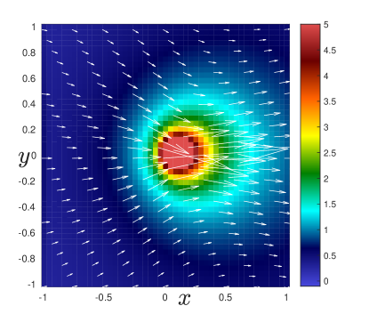
Figure 1: (a) Velocity and (b) vorticity field around a pinçon . The white arrows provide the velocity and vorticity in the plane generated by x and $\boldsymbol{\gamma}_{\alpha}$. The colour codes the out of plane velocity (a) and the logarithm in base 10 of the enstrophy (b).

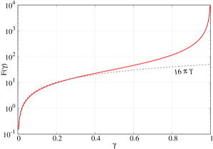
Figure 2: Parameters of a pinçon as a function of its intensity $\gamma$. (a) Intensity of the force produced by the pinçon at its location. The black dashed line has equation $y=16\pi\gamma$; (b) Generalized momentum of a pinçon . The black dashed line has equation $y=8\gamma/3$.

II.3 Properties of pinçons 

II.3.1 Scaling under coarse-graining

The velocity field and all its derivatives diverge at the location of the pinçon so they are undefined as such point. We may however study its behavior near the origin by introducing a suitable test function $\psi$ that is spherically symmetric around $x=0$, positive of unit integral, $C^{\infty}$ and that decays fast at infinity, and considering the regularizations

$$\overline{\textbf{v}_{\alpha}}^{\ell}(\textbf{x})=\int\psi\left(\frac{\textbf{x}-\textbf{y}}{\ell}\right)\textbf{v}_{\alpha}(\textbf{y})\frac{\mathrm{d}\textbf{y}}{\ell^{3}},\\$$

where $\ell$ is a small parameters. In the limit $\ell\to 0$, the function $\psi\left(\frac{\textbf{x}}{\ell}\right)$ is peaked around the origin so that, as long as x is far from $\textbf{x}_{\alpha}$, we can estimate: $\overline{\textbf{v}_{\alpha}}^{\ell}(\textbf{x})\approx\textbf{v}_{\alpha}(\textbf{x})$. Consider now the situation where $\textbf{x}=\textbf{x}_{\alpha}$. We have then:

$$\overline{\textbf{v}_{\alpha}}^{\ell}(\textbf{x}_{\alpha})=\int\psi\left(\frac{\textbf{x}_{\alpha}-\textbf{y}}{\ell}\right)\textbf{U}(\textbf{y}-\textbf{x}_{\alpha},\boldsymbol{\gamma}_{\alpha})\frac{\mathrm{d}\textbf{y}}{\ell^{3}}.\\$$

Applying finally the change of variable $\textbf{y}-\textbf{x}_{\alpha}=\ell\textbf{z}$, using homogeneity properties of U and spherical symmetry of $\psi$ we have :

$$\overline{\textbf{v}_{\alpha}}^{\ell}(\textbf{x}_{\alpha}) = \frac{1}{\ell}\int\psi\left(\textbf{z}\right)\textbf{U}(\textbf{z},\boldsymbol{\gamma}_{\alpha}){\mathrm{d}\textbf{z}},$$ (6)

$$= \frac{C_{\psi}}{\ell}\langle\textbf{v}_{\alpha}\rangle_{{\cal B}_{1}}\underset{\ell\rightarrow 0}{=}\mathcal{O}(\ell^{-1}),$$

where $C_{\psi}=4\pi\int r\psi(r)\mathrm{d}r$ and $\langle\textbf{v}_{\alpha}\rangle_{{\cal B}_{1}}$ is the average over the sphere of radius unity. Via Euler theorem, $\nabla\textbf{v}_{\alpha}$ is homogeneous of order -2. By the same reasoning, we then find that $\overline{\nabla\textbf{v}_{\alpha}}^{\ell}(\textbf{x}_{\alpha})\underset{\ell\rightarrow 0}{=}~{}\mathcal{O}(\ell^{-2})$. We cannot apply the same reasoning to $\nabla^{2}\textbf{v}_{\alpha}$ because the integral $\int\psi(r)\mathrm{d}r/r$ does not necessarily converge at the origin. However, we have the property that $\overline{(\textbf{v}_{\alpha}\cdot\mbox{${\bf\nabla}$})\textbf{v}_{\alpha}}^{\ell}+\frac{\mbox{${\bf\nabla}$}\overline{p_{\alpha}}^{\ell}}{\rho}-\nu\Delta\overline{\textbf{v}_{\alpha}}^{\ell}=\frac{\nu^{2}}{\ell^{3}}\psi\left(\frac{\textbf{x}-\textbf{x}_{\alpha}}{\ell}\right){\bf F}$ which is $\mathcal{O}(\ell^{-3})$.

II.3.2 Potential vector, vorticity and helicity

Using vector calculus identities, we can check that the velocity field around a pinçon derives from the vector potential:

$$\textbf{A}_{\alpha}(\textbf{x}) = 2\nu(\textbf{x}-\textbf{x}_{\alpha})\times\nabla\ln(\phi_{\alpha}),$$ (7)

$$= 2\nu\frac{\boldsymbol{\gamma}_{\alpha}\times(\textbf{x}-\textbf{x}_{\alpha})}{\phi_{\alpha}},$$

We can formally define the vorticity field produced locally around a pinçon by taking the curl of $\textbf{v}_{\alpha}$. The vorticity is parallel to the potential vector and reads:

$$\boldsymbol{\omega}_{\alpha}(\textbf{x})=4\nu(1-\gamma^{2})\frac{\boldsymbol{\gamma}_{\alpha}\times(\textbf{x}-\textbf{x}_{\alpha})}{\phi_{\alpha}^{3}},$$ (8)

From this, we see that the velocity field produced by a pinçon is of zero helicity.

II.3.3 Generalized Momentum and coarse-grained vorticity

We define a generalized momentum $\boldsymbol{\Pi}_{\alpha}$ for the pinçon as average of the velocity field over a sphere of unit radius (see appendix for its computation):

$$\boldsymbol{\Pi}_{\alpha}\equiv\langle\textbf{v}_{\alpha}\rangle_{{\cal B}_{1}} = \nu G(\gamma_{\alpha})\frac{\boldsymbol{\gamma}_{\alpha}}{\gamma_{\alpha}},$$

$$G(\gamma) = \frac{2}{\gamma^{2}}\left[2\gamma-(1-\gamma^{2})\ln\bigg{(}\frac{1+\gamma}{1-\gamma}\bigg{)}\right].$$ (9)

By definition, $\boldsymbol{\Pi}_{\alpha}$ provides an estimate of the coarse-grained velocity field at the pinçon position, via $\overline{\textbf{v}_{\alpha}}^{\ell}(\textbf{x}_{\alpha})=~{}C_{\psi}\boldsymbol{\Pi}_{\alpha}/\ell$. Note that $\boldsymbol{\Pi}_{\alpha}$ points in the direction of $\boldsymbol{\gamma}_{\alpha}$. For $0\leq\gamma<1$, $G(\gamma)$ varies smoothly from $0$ to $4$, starting from a linear behavior $G(\gamma)=8\gamma/3$ at the origin and ending with a vertical tangent at $\gamma=1$ (see Fig. 2-b). Therefore the function $G(\gamma)$ is bijective, and there is a one-to-one correspondance between $G$ and $\gamma$ and $\boldsymbol{\Pi}$ and $\boldsymbol{\gamma}$.

Due to the axisymmetry, we see that $\overline{\omega}^{\ell}(\textbf{x}_{\alpha})=0$, so that the coarse-grained pinçon is vorticity free near its location.

II.4 Interaction of pinçon with a regular field

There are several reasons why the notion of a ”single” pinçon does not make a physical sense:

i) the pinçon is dissipative, and requires a force to maintain it; a surrounding fluid can provide the necessary forcing;

ii) the pinçon lives in a infinite universe and does not fulfill the boundary conditions of a realistic system. To be able to use a pinçon in confined systems, we need to add an external velocity field that will take care of the boundary conditions;

iii) if we accept that the pinçon describes the very intermittent part of the energy transfer that cannot be resolved, we must also accept the possibility of coexistence and interaction of several pinçons . If we assume that the pinçons are distincts and that they are regular everywhere except at their position, this amounts again to consider the interaction of a pinçon with a regular field.

Given the nonlinear nature of the Navier-Stokes equations, we cannot superpose two solutions of Navier-Stokes equations (a pinçon and a regular field) to get a solution of Navier-Stokes equations. Instead, we will now assume that the pinçon has a dynamics and find such dynamics by imposing that the superposition of the pinçon and of the regular field obeys locally the Navier-Stokes equations. Specifically, we consider a solution of the shape $\textbf{v}_{\alpha}=\textbf{U}(\textbf{x}-\textbf{x}_{\alpha}(t),\boldsymbol{\gamma}_{\alpha}(t))$ and ${\bf F}=F(\gamma(t)){\bf e(t)}$, where $F$ is a prescribed function, and $\textbf{x}_{\alpha}$, $\boldsymbol{\gamma}=\gamma\bf{e}$, two vectors that parametrize the field $\textbf{v}_{\alpha}$ as a function of $t$. We then introduce $\textbf{v}=\textbf{v}_{\text{R}}+\textbf{v}_{\alpha}$, where $\textbf{v}_{\text{R}}$ is a velocity field that is regular at the origin, and we impose that v is a solution of Navier-Stokes locally around the singularity at $\textbf{x}_{\alpha}$, i.e. that v is a solution of

$$\partial_{t}\overline{\textbf{v}}^{\ell}(\textbf{x}_{\alpha})+\overline{(\textbf{v}\cdot\mbox{${\bf\nabla}$})\textbf{v}}^{\ell}(\textbf{x}_{\alpha})+\frac{\overline{\mbox{${\bf\nabla}$}p}^{\ell}(\textbf{x}_{\alpha})}{\rho}-\nu\overline{\Delta\textbf{v}}^{\ell}(\textbf{x}_{\alpha})=0.$$ (10)

Decomposing the velocity field into its regular and irregular part, we see that Eq. (10) generates terms of various orders in $\ell$, that scale according to Table 1. Note that since $\textbf{v}_{\text{R}}$ is a regular field, its coarse-graining scales like $O(1)$, so do its derivatives. Furthermore, we introduce the quantity $\tau^{\ell}=\overline{\textbf{v}_{\text{R}}}^{\ell}\overline{\textbf{v}_{\text{R}}}^{\ell}-\overline{\textbf{v}_{\text{R}}\textbf{v}_{\text{R}}}^{\ell}$ which is the Reynolds stress contribution due to filtering. This term has a different scaling. Indeed, $\nabla\cdot\tau^{\ell}=~{}\mathcal{O}(\delta\boldsymbol{v}_{\ell}^{2}/\ell)$ EyinkLN , where $\delta\boldsymbol{v}_{\ell}=~{}\textbf{v}_{\text{R}}(\textbf{x}+~{}\ell)-~{}\textbf{v}_{\text{R}}~{}(\textbf{x})$. Since $\textbf{v}_{\text{R}}$ is regular, it can be expanded as $\textbf{v}_{\text{R}}(\textbf{x}+~{}\ell)-~{}\textbf{v}_{\text{R}}(\textbf{x})=~{}\ell\mbox{${\bf\nabla}$}\textbf{v}_{\text{R}}$, so that $\nabla\cdot\tau^{\ell}\sim\ell(\mbox{${\bf\nabla}$}\textbf{v}_{\text{R}})^{2}=O(\ell)$.

Collecting the different term we find that the l.h.s. of Eq. (10) is the sum of the following orders:

$$\mathcal{O}(\ell) :-\nabla\cdot\tau^{\ell}$$ (11)

$$\mathcal{O}(1) :\partial_{t}\overline{\textbf{v}_{\text{R}}}^{\ell}+\mbox{${\bf\nabla}$}\cdot\overline{\textbf{v}_{\text{R}}}^{\ell}\overline{\textbf{v}_{\text{R}}}^{\ell}+\frac{\mbox{${\bf\nabla}$}\overline{p_{\text{R}}}^{\ell}}{\rho}-\nu\Delta\overline{\textbf{v}_{\text{R}}}^{\ell}$$ (12)

$$\mathcal{O}(1/\ell) :\dot{\boldsymbol{\gamma}}\boldsymbol{\mbox{${\bf\nabla}$}}_{\gamma}\overline{\textbf{v}_{\alpha}}^{\ell}+\overline{(\textbf{v}_{\alpha}\cdot\mbox{${\bf\nabla}$})\textbf{v}_{\text{R}}}^{\ell}$$ (13)

$$\mathcal{O}(1/\ell^{2}) :-\dot{\textbf{x}}_{\alpha}\mbox{${\bf\nabla}$}_{\textbf{x}}\overline{\textbf{v}_{\alpha}}^{\ell}+\overline{(\textbf{v}_{\text{R}}\cdot\mbox{${\bf\nabla}$})\textbf{v}_{\alpha}}^{\ell}$$ (14)

$$\mathcal{O}(1/\ell^{3}) :\overline{(\textbf{v}_{\alpha}\cdot\mbox{${\bf\nabla}$})\textbf{v}_{\alpha}}^{\ell}+\frac{\mbox{${\bf\nabla}$}\overline{p_{\alpha}}^{\ell}}{\rho}-\nu\Delta\overline{\textbf{v}_{\alpha}}^{\ell}$$ (15)

$\textbf{v}_{\alpha}$	$\dot{\boldsymbol{\gamma}_{\alpha}}\partial_{\gamma}(\textbf{v}_{\alpha})$	$\dot{\textbf{x}}_{\alpha}\partial_{x}\textbf{v}_{\alpha}$	$(\textbf{v}_{\alpha}\cdot\mbox{${\bf\nabla}$})\textbf{v}_{\text{R}}$	$(\textbf{v}_{\text{R}}\cdot\mbox{${\bf\nabla}$})\textbf{v}_{\alpha}$	$\mbox{${\bf\nabla}$}\cdot\overline{\textbf{v}_{\text{R}}}^{\ell}\overline{\textbf{v}_{\text{R}}}^{\ell}$
$1/{\ell}$	$1/\ell$	$1/{\ell^{2}}$	$1/{\ell}$	$1/{\ell^{2}}$	$1$

Table 1: Order of the various terms appearing in equation (10) as a function of the filter length $\ell$ in the limit $\textbf{x}\to\textbf{x}_{\alpha}$.

Cancelling the $\mathcal{O}(1/\ell^{2})$ provides a first condition as:

$$\dot{\textbf{x}}_{\alpha}\mbox{${\bf\nabla}$}_{\textbf{x}}\overline{\textbf{v}_{\alpha}}^{\ell}=\overline{(\textbf{v}_{\text{R}}\cdot\mbox{${\bf\nabla}$})\textbf{v}_{\alpha}}^{\ell}.\\$$ (16)

Due to the regularity of $\textbf{v}_{\text{R}}$, we can write $\overline{(\textbf{v}_{\text{R}}\cdot\mbox{${\bf\nabla}$})\textbf{v}_{\alpha}}^{\ell}=\textbf{v}_{\text{R}}(\textbf{x}_{\alpha})\cdot\overline{\mbox{${\bf\nabla}$}\textbf{v}_{\alpha}}^{\ell}$ for small enough $\ell$. Condition (16) is then satisfied providing:

$$\dot{\textbf{x}}_{\alpha}=\textbf{v}_{\text{R}}(\textbf{x}_{\alpha}).$$ (17)

Physically, this means that the singularity point is advected by the regular field surrounding it.

Cancelling the $\mathcal{O}(1/\ell)$ provides a second condition, as:

$$\dot{\boldsymbol{\gamma}}\overline{\mbox{${\bf\nabla}$}_{\gamma}\textbf{v}_{\alpha}}^{\ell}=-\overline{(\textbf{v}_{\alpha}\cdot\mbox{${\bf\nabla}$})\textbf{v}_{\text{R}}}^{\ell}.$$ (18)

Due to the regularity of $\textbf{v}_{\text{R}}$, we can write $(\overline{\textbf{v}_{\alpha}\cdot\mbox{${\bf\nabla}$})\textbf{v}_{\text{R}}}^{\ell}=(\overline{\textbf{v}_{\alpha}}^{\ell}\cdot\mbox{${\bf\nabla}$})\textbf{v}_{\text{R}}(\textbf{x}_{\alpha})$. We then get the equation:

$$\dot{\boldsymbol{\gamma}}\overline{\mbox{${\bf\nabla}$}_{\gamma}\textbf{v}_{\alpha}}^{\ell}=-(\overline{\textbf{v}_{\alpha}}^{\ell}\cdot\mbox{${\bf\nabla}$})\textbf{v}_{\text{R}}.$$ (19)

Physically, this means that the force axis and its direction are moved around by the shear of the regular field at the location of the singularity.

Cancelling the $\mathcal{O}(1)$ term provides the condition that $\overline{\textbf{v}_{\text{R}}}^{\ell}$ is a solution of the Navier-Stokes equation. Indeed, this is the idea behind the two fluid model, to allow for the scales above the coarse-graining to be described by a solution of the Navier-Stokes equation.

We are then left with the smallest order $O(\ell^{2})$ and the highest order term $O(\ell^{-3})$, which cannot be balanced in general. For the system to have a physical solution, we then impose a ”bootstrap condition”, namely that the two terms must be of the same order of magnitude, thereby fixing the coarse-graining scale $\ell_{c}$ via $\nu^{2}/\ell_{c}^{3}\sim~{}\ell_{c}(\mbox{${\bf\nabla}$}\textbf{v}_{\text{R}})^{2}$. We thus find $\ell_{c}=(\nu^{3}/\epsilon_{r})^{1/4}$, with $\epsilon_{r}=\nu(\mbox{${\bf\nabla}$}\textbf{v}_{\text{R}})^{2}$ is the dissipation of the regular field. Therefore, the coarse-graining scale imposed by the bootstrap condition is precisely the Kolmogorov scale $\ell_{c}=\eta$.

Physically, this condition can be understood as follow: the singularity is dissipative, and to maintain it, one must apply a force. Such force is provided by the regular field, through the term $\nabla\cdot\tau^{\ell}$, which keeps track of the fraction of the velocity field that is sent to the subgrid scale, and which is taken into account by the pinçon . Conversely, the pinçon applies an extra turbulent stress onto the regular field, that extends around it in a ball of radius of the order of the Kolmogorov scale. To keep a precise account of these effects, we thus split the Reynolds stress and the pinçon force into a contribution at $\textbf{x}_{\alpha}$ and a contribution around that location, ans share the contribution among the pinçon, and the regular field.

Taking into account the fact that $\overline{\textbf{v}_{\text{R}}}^{\eta}\approx\textbf{v}_{\text{R}}$, $\overline{\textbf{v}_{\alpha}}^{\eta}=C_{\psi}\boldsymbol{\Pi}_{\alpha}/\eta$ and $\dot{\boldsymbol{\gamma}}\overline{\mbox{${\bf\nabla}$}_{\gamma}\textbf{v}_{\alpha}}^{\eta}\approx C_{\psi}\dot{\boldsymbol{\Pi}}_{\alpha}/\eta$, we then get the following system of equations to describe the coupling between the pinçon and the regular field:

for the regular field:

$$\begin{array}[]{rcl}\partial_{t}\overline{\textbf{v}_{\text{R}}}^{\eta}(\textbf{x})&+&(\overline{\textbf{v}_{\text{R}}}^{\eta}\cdot\mbox{${\bf\nabla}$})\overline{\textbf{v}_{\text{R}}}^{\eta}(\textbf{x})+\frac{\mbox{${\bf\nabla}$}\overline{p_{R}}^{\eta}}{\rho}(\textbf{x})-\nu\Delta\overline{\textbf{v}_{\text{R}}}^{\eta}(\textbf{x})\\ &=&\nabla\cdot\tau^{\eta}(\textbf{x})-\frac{\nu^{2}}{\eta^{3}}\psi\left(\frac{\textbf{x}-\textbf{x}_{\alpha}}{\eta}\right)\textbf{F}_{\alpha};\end{array}$$ (20)

for the pinçon:

$$\dot{\textbf{x}}_{\alpha} = \overline{\textbf{v}_{\text{R}}}^{\eta}(\textbf{x}_{\alpha}),$$

$$\dot{\boldsymbol{\Pi}}_{\alpha} = -(\boldsymbol{\Pi}_{\alpha}\cdot\mbox{${\bf\nabla}$})\overline{\textbf{v}_{\text{R}}}^{\eta}(\textbf{x}_{\alpha})+\frac{\eta}{C_{\psi}}\nabla\cdot\tau^{\eta}(\textbf{x}_{\alpha})-\frac{\nu^{2}\psi(0)}{C_{\psi}\eta^{2}}{\textbf{F}_{\alpha}}.$$ (21)

These equations describe a two-fluid approach of turbulence, coupling a coarse-grained field at the Kolmogorov scale, and the pinçon . The velocity fluid is follows coarse-grained Navier-Stokes equations, with the Reynolds stress providing the necessary driving force to create pinçons . The latter are entities living below the Kolmogorov scale, that are advected and sheared by the coarse-grained fluid, and exert back a forcing on the coarse-grained field, that results in a dissipation of energy. To conclude our two-fluid model, we must prescribe the interactions between pinçons , in a way that is compatible with the Navier-Stokes equations.

II.5 Interactions of pinçons 

An ensemble of $N$ pinçons , $\alpha=1...N$ produces a velocity field $\textbf{v}(x,t)$:

$$\textbf{v}(x,t)=\sum_{\alpha}\textbf{v}_{\alpha}(x,t),$$ (22)

Around a pinçon   $\alpha$, the ensemble of other pinçons produces a regular field $\textbf{v}_{\text{R}}=~{}\sum_{\beta\neq\alpha}\textbf{v}_{\beta}(\textbf{x}_{\alpha})$. Motivated by such observation, we define the interactions of the pinçons via the following set of $2N$ differential equations:

$$\dot{\textbf{x}}_{\alpha} = \sum_{\beta\neq\alpha}\textbf{v}_{\beta}(\textbf{x}_{\alpha},t),$$ (23)

$$\dot{\boldsymbol{\Pi}}_{\alpha} = -(\boldsymbol{\Pi}_{\alpha}\cdot\mbox{${\bf\nabla}$}_{\textbf{x}_{\alpha}})\bigg{(}\sum_{\beta\neq\alpha}\textbf{v}_{\beta}(\textbf{x}_{\alpha},t)\bigg{)}-\frac{\nu^{2}\psi(0)}{C_{\psi}\eta^{2}}\textbf{F}_{\alpha}+\frac{E_{\alpha}}{C_{\psi}}\chi,$$ (24)

where $E_{\alpha}=U_{\alpha}^{2}$ describes the local energy of the large scale regular field that provides a stochastic forcing $\chi$ via the (random) Reynolds stress contribution. In the sequel, we assume that $\chi$ is isotropic and shortly correlated over a a Kolmogorov time scale, so that $\langle\chi_{i}(t)\chi_{j}(t^{\prime})\rangle=~{}\delta(t-~{}t^{\prime})\delta_{ij}$. Note that the equation (24) is a definition, that leaves aside many conditions that may have to be satisfied for the model to be an exact representation of the small scales of Navier-Stokes. For example, this model is more likely to be valid as the dilute limit is achieved, so that the pinçons are sufficiently apart from each other for them to be considered as ponctual particles. Also, we do not try to make a difference between close and distant interactions, while in the former case, diverging velocities and correlations may impede our possibility to consider that the field generated by the external fields is smooth enough so that the approximation $\overline{(\textbf{v}_{\text{R}}\cdot\mbox{${\bf\nabla}$})\textbf{v}_{\alpha}}^{\ell}=\textbf{v}_{\text{R}}(\textbf{x}_{\alpha})\cdot\overline{\mbox{${\bf\nabla}$}\textbf{v}_{\alpha}}^{\ell}$ is valid for small enough $\ell$. Therefore, even if individually each pinçon is a weak solution of Navier-Stokes equations, the collection of N pinçon is not an exact weak solution of Navier-Stokes equations.

In some sense anyway, the equations of motions of the pinçons correspond to the equations that are imposed by the structure of the Navier-Stokes equations and the requirement that the local velocity field induced by each pinçon should obey such equations. Eqs. (24) can therefore be seen as the equivalent of the motion of poles or zeros of partial differential equations that have been computed, starting from KruskalKruskal74 for the KdV equations (see Calogero96 ; Calogero01 for a review). The motions are furthermore constrained by the condition that they stay with the unit hypersphere such that $\|\boldsymbol{\gamma}_{\alpha}\|<1$.

The pinçon are characterized by an interaction energy:

$$E=\frac{C_{\psi}}{\eta}\sum_{\beta\neq\alpha}\boldsymbol{\Pi}_{\alpha}\cdot\textbf{v}_{\beta}(\textbf{x}_{\alpha},t).$$ (25)

Due to the presence of dissipation and forcing $\textbf{F}_{\alpha}$ and $\chi$, this interaction energy is not conserved in general. However, there may exist situations where dissipation and forcing balance statistically, so that the system reaches an out-of-equilibrium steady state.

II.6 Weak pinçon limit

The equations of motions (24) takes a simple expression, in the ”weak pinçon ” limit, where the intensity of the pinçons are very small, $\gamma_{\alpha}\ll 1$ for any $\alpha$. In this case, $\boldsymbol{\Pi}_{\alpha}=8\nu\boldsymbol{\gamma}_{\alpha}/3$ and one can develop $\phi_{\alpha\beta}^{-1}=(1+\boldsymbol{\gamma}_{\beta}\cdot\textbf{r}_{\alpha\beta}/\|\textbf{r}_{\alpha\beta}\|)$. The equations of motions under such approximations are :

$$\dot{\textbf{x}}_{\alpha} = 2\nu\sum_{\beta\neq\alpha}\left[\frac{\boldsymbol{\gamma}_{\beta}}{\|\textbf{r}_{\alpha\beta}\|}+\left(\boldsymbol{\gamma}_{\beta}\cdot\textbf{r}_{\alpha\beta}\right)\frac{\textbf{r}_{\alpha\beta}}{\|\textbf{r}_{\alpha\beta}\|^{3}}\right],$$

$$\dot{\boldsymbol{\gamma}}_{\alpha} = 2\nu\sum_{\beta\neq\alpha}\left[-(\boldsymbol{\gamma}_{\alpha}\cdot\boldsymbol{\gamma}_{\beta})\frac{\textbf{r}_{\alpha\beta}}{\|\textbf{r}_{\alpha\beta}\|^{3}}+3\,(\boldsymbol{\gamma}_{\alpha}\cdot\textbf{r}_{\alpha\beta})(\boldsymbol{\gamma}_{\beta}\cdot\textbf{r}_{\alpha\beta})\frac{\textbf{r}_{\alpha\beta}}{||\textbf{r}_{\alpha\beta}||^{5}}\right.$$

$$\left.-\,\boldsymbol{\gamma}_{\alpha}\frac{\boldsymbol{\gamma}_{\beta}\cdot\textbf{r}_{\alpha\beta}}{\|\textbf{r}_{\alpha\beta}\|^{3}}+\boldsymbol{\gamma}_{\beta}\frac{\boldsymbol{\gamma}_{\alpha}\cdot\textbf{r}_{\alpha\beta}}{\|\textbf{r}_{\alpha\beta}\|^{3}}\right]-\frac{6\pi\nu\psi(0)}{C_{\psi}\eta^{2}}\boldsymbol{\gamma}_{\alpha}+\frac{3E_{\alpha}}{8C_{\psi}\nu}\chi.$$

These equations of motions are reminiscent of the equations of motions of the vortons (see Eq. (46) in Appendix), with vectorial products being replaced by scalar product, and additional terms appearing. However, the motion and intensities of the pinçons are driven by forces decaying respectively like $1/r$ and $1/r^{2}$, rather than respectively $1/r^{2}$ and $1/r^{3}$ for the vortons. Moreover, the pinçons are subject to a friction proportional to the viscosity.

The interaction energy in this case is:

$$E=\frac{16C_{\psi}\nu^{2}}{3\eta}\sum_{\beta\neq\alpha}\left[\frac{\boldsymbol{\gamma}_{\alpha}\cdot\boldsymbol{\gamma}_{\beta}}{\|\textbf{r}_{\alpha\beta}\|}+\frac{\left(\boldsymbol{\gamma}_{\alpha}\cdot\textbf{r}_{\alpha\beta}\right)\left(\boldsymbol{\gamma}_{\beta}\cdot\textbf{r}_{\alpha\beta}\right)}{\|\textbf{r}_{\alpha\beta}\|^{3}}\right],$$ (27)

which is the classical self interaction energy of pair of singularities Pedrizzetti1992 .

III Dynamics of a pair of pinçons 

III.1 Interest of considering pair of pinçons 

Previous experimental [S16]; debue2021 and numerical investigations Nguyen20 about the location of the structures with extreme local energy transfer showed that they are located near interactions (possibly reconnection) of Burgers vortices. Previous and recent high-resolution numerical simulations of reconnection of anti-parallel vorticity filaments Kerr89 ; yao_hussain_2020 showed that the process is associated with the formation of a local cusp over each filament, that could possibly lead to a singular behaviour yao20 . This possibility was confirmed by a detailed study of the interaction of two Burgers vortices conducted by Kimura18 ; moffatt_kimura_2019 ; moffatt_kimura_2019_2 ; Moffatt20 ; Kimura_2017 using the Biot-Savart approximation. They showed that the interaction indeed leads to a cusp formation on the vortex line, with very large, possibly diverging velocities at the tip of the cusp, with orientation along the bisector of the angle of the cusp. The reconnection was also found to be associated with a depletion of the helicity, that eventually reaches zero at the reconnection Kimura18 .  In this picture, the associated pinçons created by a coarse-graining at the Kolmogorov scale would then be located at the tip of each cusp, with spins in the direction of the bisector of the cusps (see Figure 3-(a)). This shows the interest of studying more closely the dynamics of a pair of pinçons and see how it compares with known features of the reconnection. This is the aim of the present section. In all the sequel, we renormalize the length by $r_{0}$, the distance between the two pinçons at time $t=0$ and the time by the associated viscous time $\tau_{\nu}=\textbf{r}_{0}^{2}/\nu$. We first start with the simplest case, where the pair constitutes a dipole.

III.2 Dynamics of a dipole of pinçons 

III.2.1 Equations

Figure 3: (a) Schematic geometry of pinçons creation at reconnection. (b) Geometry of the dipole: two pinçons located at $\textbf{x}_{\alpha}$ and $\textbf{x}_{\beta}$, and such that initially $\boldsymbol{\gamma}_{\alpha}+\boldsymbol{\gamma}_{\beta}=0$. By convention, the angle $\theta$ is the angle between $\boldsymbol{\gamma}_{\alpha}$ and $\textbf{r}=\textbf{x}_{\alpha}-\textbf{x}_{\beta}$. The figure (a) is adapted from figure 3 of yao_hussain_2020 .

Let us consider the dynamics of a dipole, sketched in Figure 3-(b), made of two pinçons located at $\textbf{x}_{\alpha}$ and $\textbf{x}_{\beta}$, and such that initially $\boldsymbol{\gamma}_{\alpha}+\boldsymbol{\gamma}_{\beta}=0$ and $\textbf{x}_{\alpha}-\textbf{x}_{\beta}=r_{0}\textbf{r}$ . We have then $\textbf{v}_{\beta}(\textbf{x}_{\alpha})=-\textbf{v}_{\alpha}(\textbf{x}_{\beta})\equiv\nu\textbf{V}(\textbf{r})/r_{0}$ and $\textbf{F}_{\alpha}+\textbf{F}_{\beta}=0$. Using the aforementioned non-dimensionalization, we then get the equation of motions:

$$\dot{\textbf{x}}_{\alpha} = \frac{\nu}{r_{0}}\textbf{V},$$

$$\dot{\textbf{x}}_{\beta} = -\frac{\nu}{r_{0}}\textbf{V},$$

$$\dot{\boldsymbol{\Pi}}_{\alpha} = \boldsymbol{\Pi}_{\alpha}\nabla_{r}\boldsymbol{V}-\frac{\nu\psi(0)}{C_{\psi}}\left(\frac{r_{0}}{\eta}\right)^{2}\textbf{F}_{\alpha}+\frac{kT_{\alpha}r_{0}^{2}}{C_{\psi}\nu}\chi,$$ (28)

$$\dot{\boldsymbol{\Pi}}_{\beta} = -\boldsymbol{\Pi}_{\beta}\nabla_{r}\boldsymbol{V}-\frac{\nu\psi(0)}{C_{\psi}}\left(\frac{r_{0}}{\eta}\right)^{2}\textbf{F}_{\beta}+\frac{kT_{\beta}r_{0}^{2}}{C_{\psi}\nu}\chi.$$

Therefore, the center of mass of the dipole $\textbf{x}_{\alpha}+\textbf{x}_{\beta}$ does not move, while the mean dipole strength $(\boldsymbol{\Pi}_{\alpha}+\boldsymbol{\Pi}_{\beta})/2$ obeys:

$$\dot{\boldsymbol{\Pi}}_{\alpha}+\dot{\boldsymbol{\Pi}}_{\beta}=\frac{(E_{\alpha}+E_{\beta})r_{0}^{2}}{2C_{\psi}\nu}\chi.$$ (29)

We see that he forcing induces fluctuations proportional to the mean local energy $(E_{\alpha}+E_{\beta})/2$ that destroy the dipole geometry over a viscous time scale. It therefore only make sense to study the dipole case in the low temperature limit where $(E_{\alpha}+E_{\beta})/2\to 0$.

III.2.2 Results at zero temperature

Let us first investigate the dynamics in the zero temperature $E_{\alpha}+E_{\beta}=0$. In this case, the dipole remains exactly a dipole at all times and we have $\boldsymbol{\Pi}_{\alpha}=-\boldsymbol{\Pi}_{\beta}\equiv\nu\boldsymbol{\Pi}$, $\textbf{F}_{\alpha}=-\textbf{F}_{\beta}\equiv~{}\textbf{F}$ and $\boldsymbol{\gamma}_{\alpha}=~{}-~{}\boldsymbol{\gamma}_{\beta}\equiv~{}\boldsymbol{\gamma}$. The dipole dynamics of the quantities characterizing the dipole, namely r and $\boldsymbol{\gamma}$ (or equivalently $\boldsymbol{\Pi}$), can be obtained by taking the difference of the first two and the last two equations of Eq. (28) to get:

$$\dot{\textbf{r}} = 4\left(-\frac{\boldsymbol{\gamma}+\textbf{r}/r}{r\phi_{*}}+(1-\gamma^{2})\frac{\textbf{r}}{r^{2}\phi_{*}^{2}}\right),$$ (30)

$$\dot{\boldsymbol{\Pi}} = \frac{2\Pi}{r^{3}\phi_{*}^{3}}A(\gamma,\theta)\,\boldsymbol{r}-\frac{\psi(0)}{C_{\psi}}\left(\frac{r_{0}}{\eta}\right)^{2}\textbf{F},$$ (31)

where

$$A(\gamma,\theta)=\gamma\left(1-3\cos^{2}(\theta)-3\gamma\cos(\theta)-\gamma\cos^{3}(\theta)-2\gamma^{2}\right)$$ (32)

where $r=\|\textbf{r}\|$, $\cos(\theta)=(\boldsymbol{\gamma}\cdot\textbf{r})/(r\gamma)$, $\phi_{*}=1+\gamma\cos(\theta)$ and $\Pi=\|\boldsymbol{\Pi}\|=G(\gamma)$.

From these expressions, we see that the evolution of r and $\boldsymbol{\Pi}$ remains in the plane generated by the two vectors r and $\boldsymbol{\gamma}$. We are then left with only 3 independent quantities to determine the dipole axis and its orientation, namely $r$, $\theta$ and $\gamma$. The evolution of the first two quantities can be simply derived by projecting Eq. (30) on $\textbf{e}_{r}$ and $\textbf{e}_{\theta}$, while the last quantity can be obtained by taking the scalar product of Eq. (31) with $\boldsymbol{\Pi}$ to get an evolution for $\|\boldsymbol{\Pi}\|^{2}$, which leads to $\gamma$ through $\gamma=G^{-1}(\|\boldsymbol{\Pi}\|)$. We thus get after straightforward simplifications:

$$\dot{r} = \frac{4}{r}\left(\frac{1-\gamma^{2}}{\phi_{*}^{2}}-1\right),$$ (33)

$$r\dot{\theta} = 4\,\frac{\gamma\sin\theta}{r\phi_{*}},$$ (34)

$$\dot{\boldsymbol{\Pi}^{2}} = 4\frac{\Pi^{2}}{r^{2}}A(\gamma,\theta)\cos(\theta)-\frac{2\psi(0)}{C_{\psi}}\left(\frac{r_{0}}{\eta}\right)^{2}\textbf{F}\cdot\boldsymbol{\Pi}$$ (35)

We have integrated the equations of motions (35) for fixed initial radius $r_{0}=1$ and $\gamma_{0}=0.1$ and various initial values of $\theta_{0}$ and taking $\psi(0)=1/(2\pi)^{3/2}$ (valid for $\psi$ Gaussian). The resulting evolutions are computed in two case, with and without friction. The first case corresponds to the initial stage of the dynamics, just after the pinçons are created. Indeed, a pinçon is created with an initial force corresponding to the local Reynolds stress $\textbf{F}_{\alpha}=\eta^{3}/(\nu^{2}\psi(0))\nabla\cdot\tau^{\eta}(\textbf{x}_{\alpha})$, so that the dissipation is initially suppressed. In that case, we observe in Fig. 4-a that there are two fixed points of the dynamics for $\theta$: one stable and attractive, corresponding to $\theta=\pi$, and one unstable and repelling, corresponding to $\theta=0$. As a result, the pinçons are mostly repelling each other, except when they start exactly anti-aligned and facing away each other, in which case they attract each other and anihiliate each other. The resulting dynamics can also be appreciated in the phase space, as shown in figure 5-a.

Interesting scaling laws are observed in the two stages, that are reminiscent of what is observed during reconnection events The pinçons with initial inclination in the interval $[0,\pi/2]$ and different from $0$ start moving towards each other, while decreasing their strength and increasing their angle, in absolute value. Once they reach the value $\theta=\pi/2$, they change direction and get away from each other (see figure 6-a). During the collapse stage, the radius of the dipole decreases approximately like like $\sqrt{t_{c}-t)}$, which is the Leray scaling Leray34 ). The collapse stage is nearly universal, with weak dependance on the initial angle, while the escape depends more strongly on the initial orientation. Such asymmetry has been also observed in reconnection of quantum vortices Villois20 . During the separating stage, $\theta$ gets closer to $\pi$ and there is also an approximate power law escape law $r\sim\sqrt{t-t_{c})}$. The scaling laws are explored further in the general case, in section 3.d.

At a later stage, the initial Reynolds stress has decayed and cannot balance anymore the pinçons dissipation. The extreme case is when the Reynolds stress has decayed to zero, and when the dissipation is the strongest. This case has been studied by running another set of simulation including the friction, starting the dipole at $r_{0}=\eta$. It is shown in Figure 4-(b). We see that, as expected, the dissipation now induces a constant decline of the dipole intensity, that eventually results in the death of the dipole. The resulting phase space is shown in figure 5-b, where a plunging funnel corresponding to dissipation can now clearly be seen. There are now two situations depending on whether the initial angle is less or bigger than $\pi/2$ . In the first case, the dipole contracts and orientates itself towards $\pi/2$ before its death. This situation can be associated to a reconnection event. For initial angles greater than $\pi/2$, the dipole expands while keeping its initial orientation before eventually dying and stopping.

Summarizing, the natural dynamics of a dipole without stochastic forcing is always dissipative, resulting in the final death of the dipole. Before its death, the dipole can experience either a first contraction stage of its initial angle is less than $\pi/2$, with dynamics resembling reconnection event, or experiences and expansion while it tries to anti-align its two components ($\theta\to\pi$). The question is now whether the dipole can be maintained for a longer time, and maintain another orientation if we take the stochastic forcing into account. As we showed in the beginning, as soon as we add some stochastic noise, the dipolar geometry breaks down in a viscous time scale. There is therefore a subtle interplay to be understood between the decay of the dipole, the forcing and the departure from dipolar geometry. There is however an interesting observation, that allows to tackle the problem in a simple and elegant manner. Indeed, due to the friction, the pinçon intensity decreases with time, and we are likely to enter into the weak pinçon limit after a sufficient long time. The latter is much simpler to code and understand, since it ressembles the dynamics of dipolar moments. In the sequel, we therefore investigate the finite but small forcing limit in the weak pinçon approximation.

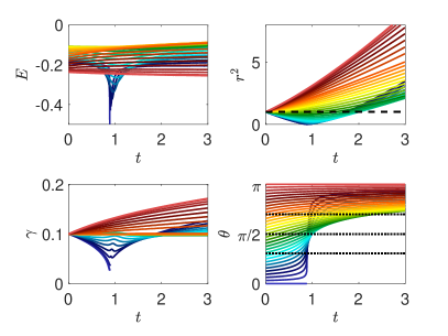
Figure 4: Dynamics of a dipole of pinçon for various initial conditions and (a) Without friction, corresponding to the initial stage of the dynamics, just after pinçons creation; (b) With friction, corresponding to the late stage dynamics. The radius is initially fixed to $r=1$, the dipole intensity is initially set to $\gamma=0.1$ and the initial dipole orientation is fixed at different values between $0$ and $\pi$. The panel represent the time evolution of the different quantities: $E$: Interaction energy; $r^{2}$: Square of Dipole separation; $\gamma$: Dipole intensity; $\theta$: Dipole orientation. Black dashed lines on $\theta(t)$ figure correspond to $\arccos\big{(}\frac{1}{\sqrt{3}}\big{)},\frac{\pi}{2}$, and $\pi-\arccos\big{(}\frac{1}{\sqrt{3}}\big{)}$.

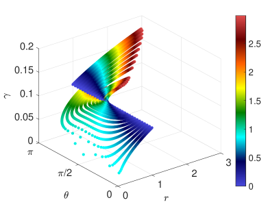
Figure 5: Phase space for a dipole of pinçons color-coded by the time, shown on the color bar. (a) Without friction, corresponding to the initial stage of the dynamics, just after pinçons creation (b) With friction, corresponding to the late stage dynamics. The radius is initially fixed to $r=1$, the dipole intensity is initially set to $\gamma=0.1$ and the initial dipole orientation is fixed at different values between $0$ and $\pi$.

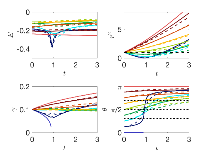
Figure 6: Comparison with the weak limit approximation: solid lines: complete model; dashed line: weak limit; (a)Without friction. (b) With friction. The panel represent the time evolution of the different quantities: $E$: Interaction energy; $r^{2}$: Square of Dipole separation; $\gamma$: Dipole intensity; $\theta$: Dipole orientation. Black dashed lines on $\theta(t)$ figure correspond to $\arccos\big{(}\frac{1}{\sqrt{3}}\big{)},\frac{\pi}{2}$, and $\pi-\arccos\big{(}\frac{1}{\sqrt{3}}\big{)}$.

III.3 Results at finite small temperature

III.3.1 From pair of pinçons to dipole equations in the weak pinçon limit

In such limit, we can obtain the dipole dynamics and the evolution of the dipole radius, orientation and strength from the evolution of three quantities: $R=r^{2}$, $C=\boldsymbol{\gamma}\cdot\textbf{r}$ and $N=\boldsymbol{\gamma}^{2}$. To obtain them, we first write the equations Eq. (II.6) for two pinçons  $\boldsymbol{\gamma}_{\alpha}$ and $\boldsymbol{\gamma}_{\beta}$, and introduce three quantities: $\textbf{r}=\textbf{x}_{\alpha}-\textbf{x}_{\beta}$, ${\boldsymbol{\Gamma}}=(\boldsymbol{\gamma}_{\alpha}+\boldsymbol{\gamma}_{\beta})/2$ and ${\boldsymbol{\Pi}}=(\boldsymbol{\gamma}_{\alpha}-\boldsymbol{\gamma}_{\beta})/2$. By combination of the equations of motions, we obtain 3 coupled equations:

$${\dot{\textbf{r}}} = -4\nu\left(\frac{{\boldsymbol{\Pi}}}{r}+\textbf{r}\frac{{\boldsymbol{\Pi}}\cdot\textbf{r}}{r^{3}}\right),$$

$${\dot{\boldsymbol{\Pi}}} = 2\nu\left[\left(\Pi^{2}-\Gamma^{2}\right)\frac{\textbf{r}}{r^{3}}+3\frac{\textbf{r}}{r^{5}}\left(({\boldsymbol{\Gamma}}\cdot\textbf{r})^{2}-({\boldsymbol{\Pi}}\cdot\textbf{r})^{2}\right)\right]-\frac{6\pi\nu\psi(0)}{C_{\psi}\eta^{2}}{\boldsymbol{\Pi}}+\frac{3(E_{\alpha}-E_{\beta})}{16C_{\psi}\nu}\chi,$$ (36)

$$\dot{\boldsymbol{\Gamma}} = 4\nu\left[{\boldsymbol{\Gamma}}\frac{({\boldsymbol{\Pi}}\cdot\textbf{r})}{r^{3}}-{\boldsymbol{\Pi}}\frac{({\boldsymbol{\Gamma}}\cdot\textbf{r})}{r^{3}}\right]-\frac{6\pi\nu\psi(0)}{C_{\psi}\eta^{2}}{\boldsymbol{\Gamma}}+\frac{3(E_{\alpha}+E_{\beta})}{16C_{\psi}\nu}\chi.$$

The last equation of Eq. (III.3.1) shows that ${\boldsymbol{\Gamma}}$ is forced by $\bar{E}=(E_{\alpha}+E_{\beta})/2$. If we start with a dipole condition $\Gamma=0$. In the small temperature limit $\bar{E}\ll 1$ and for time scale short with respect to the diffusive time scale $\tau_{\nu}=r_{0}^{2}/\nu$, we can then ignore all the terms proportional to $\Gamma$ in the second equation of Eq. (III.3.1). We then multiply the first equation by r and the second equation by ${\boldsymbol{\Pi}}$ to obtain equations for $R$ and $N$, and we sum the first equation multiplied by ${\boldsymbol{\Pi}}$ with the second equation multiplied by r to get the equation of evolution for $C$. After non-dimensionalization by $r_{0}$ and $r_{0}^{2}/\nu$ and rearrangement, we then obtain the 3 coupled equations:

$${\dot{R}} = -16\frac{C}{R^{1/2}},$$

$${\dot{C}} = -2\left[\frac{N}{R^{1/2}}+5\frac{C^{2}}{R^{3/2}}\right]-\rho C+R^{1/2}\mu\zeta,$$ (37)

$${\dot{N}} = 4\left[N\frac{C}{R^{3/2}}-3\frac{C^{3}}{R^{5/2}}\right]-\rho N+N^{1/2}\mu\zeta,$$

where $\zeta$ is a delta correlated white noise obeying $<\zeta(t)\zeta(t^{\prime})>=\delta(t-t^{\prime})$, and the friction $\rho$ and forcing $\mu$ coefficient are given by

$$\begin{array}[]{rcl}\mu&=&\frac{3r_{0}^{2}(E_{\alpha}-E_{\beta})}{16\nu^{2}C_{\psi}},\\ \rho&=&6\pi\psi(0)\frac{r_{0}^{2}}{\eta^{2}C_{\psi}}.\end{array}$$ (38)

From $N$, $R$ and $C$, we then get $r=R^{1/2}$, $\gamma=N^{1/2}$ and $\theta=\mathrm{\arccos}(C/(r\gamma)$.

To check the validity of the weak limit approximation, we show in Figure 6 the comparison between the full dynamics computed from Eq. (31) and its weak limit Eq. (III.3.1) in the zero temperature limit $\mu=0$ and without ($\rho=0$) and with friction. We see that the two dynamics coincide very well for most cases, and that the approximation is better on the late stage, when there is friction. Indeed, the friction forces decay of the dipole intensity.

The weak dipole limit actually helps us identifying special angles for the dipole dynamics. Indeed, from the last equation of Eq. (III.3.1), we see that the first term of the r.h.s cancels whenever $\xi(\theta)=\cos(\theta)\big{(}1-3\cos^{2}(\theta)\big{)}=0$, corresponding to the three angles in the interval $[0,\pi]$, namely $\theta=\pi/2$, $\theta=\arccos(1/\sqrt{(}3))$ and $\theta=\pi-\arccos(1/\sqrt{(}3))$. Those angles are identified by black dotted lines in figures 4, 6, 7. When the forcing and dissipation vanish or balance, they correspond to special directions where the dipole intensity can remain stationary. We see that indeed, the angle $\theta=\pi/2$ partitions the dynamics since the angles $\theta(t)$ increase and the radius decreases if and only if $\theta(t)$ is smaller than $\frac{\pi}{2}$. The two other angles do not seem to play a specific role in the zero temperature limit. However, the situation is different in the other situation, at finite temperature, as we now show.

III.3.2 Dynamics at finite temperature

Integrating (III.3.1) allows to efficiently study the dynamic of a noisy dipole, provided two criteria are satisfied: i) $\gamma\leq 0.5$, in order to be in the weak limit and ii) $r$ is large enough ($r\geq\frac{1}{\sqrt{\rho}}$) so that the two pinçons may still be considered as distinct Moreover, for numerical reasons, we stop the integration whenever $\gamma\leq 0.01$ or $r\geq\sqrt{\rho}$, in which case we consider that the pinçons are either dying or that the dipole has escaped to infinity. In practise, most of our simulations were stopped because either $\gamma\leq 0.01$ or $\gamma\geq 0.5$. Figure 7 shows the evolution a dipole satisfying of the equations of motions (III.3.1) for fixed initial radius $r_{0}=1$ and $\gamma_{0}=0.1$, various initial values of $\theta_{0}$ and $\rho=0.12$ and $\mu=0.009$. Several tendencies emerge, as illustrated in figure 7. First the integration time is slightly longer as the noise may maintain $\gamma$ stationary for a certain amount of time. Second, the evolution of $\theta(t)$ is not monotonic anymore and the angle $\theta$ tends to get closer to the values cancelling $\xi(\theta)$, and tend to $\theta=\pi/2$ in most of the cases. As a result, the dipole can be maintain for some time in a non-equilibrium balance, where dissipation exactly balances the stochastic forcing, allowing the dipole intensity to decay less rapidly, and the dipole to live longer. In the phase space diagram ($r$, $\theta$, $\gamma$) trajectories with noise tends to allow the movement longer, keeping a larger $\gamma$ and leading to values of $\theta$ closer to $\pi$. In the low noise regime, noise can therefore be a source of stimulation keeping the dipole alive and slowing down its death.

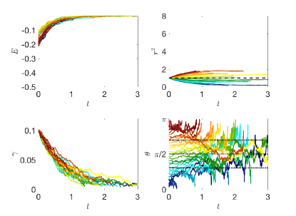
Figure 7: Effect of noise in the weak limit dissipative case (a) on the dynamics. The panel represent the time evolution of the different quantities: $E$:Interaction energy; $r^{2}$ Square of Dipole separation; $\gamma$: Dipole intensity; $\theta$: Dipole orientation. Black dashed lines on $\theta(t)$ figure correspond to $\arccos\big{(}\frac{1}{\sqrt{3}}\big{)},\frac{\pi}{2}$, and $\pi-\arccos\big{(}\frac{1}{\sqrt{3}}\big{)}$; (b) on the phase-space, color-coded by the time, shown on the color bar.The radius is initially fixed to $r=1$, the dipole intensity is initially set to $\gamma=0.1$ and the initial dipole orientation is fixed at different values between $0$ and $\pi$. The intensity of the noise is $\mu=0.009$

We have checked that when the noise is too large, then fluctuations are enough to bring the dipole intensity close to the limit $\gamma=0$ or $\gamma=1$ in a finite time, resulting in the dipole collapse or death quicker than in the zero temperature limit.

III.4 General dynamics of a pair of pinçons 

III.4.1 Short time dynamics

In the case of dipole, the short time dynamics corresponds either to an escape with $\theta\to\pi$ and $\gamma\to 1$ or first a contraction (close interaction) and than an escape. Here we consider the general case of a pair of pinçons to determine whether such observation is robust or not. The relative dynamics is characterized in this case by 6 independent scalar variables which are the distance $r$ between the pinçons , their intensities $\gamma_{\alpha}$ and $\gamma_{\beta}$, their angles $\theta_{\alpha}$ and $\theta_{\beta}$ defined by $\mathrm{cos}\,\theta_{\alpha}=(\boldsymbol{\gamma}_{\alpha}\cdot\textbf{r}_{\alpha\beta})/(r\gamma_{\alpha})$ and $\mathrm{cos}\,\theta_{\beta}=(\boldsymbol{\gamma}_{\beta}\cdot\textbf{r}_{\beta\alpha})/(r\gamma_{\beta})$ and the angle $\varphi$ defined by $\mathrm{cos}\,\varphi=(\boldsymbol{\gamma}_{\alpha}\cdot\boldsymbol{\gamma}_{\beta})/(\gamma_{\alpha}\gamma_{\beta})$. The dipole case studied in the previous section corresponds to $\gamma=\gamma_{\alpha}=\gamma_{\beta}$ , $\theta=\theta_{\alpha}=\theta_{\beta}$ and $\varphi=\pi$. We then integrate the dynamics with equations (24) without dissipation and noise for different initial conditions of these parameters, except that we always set $r_{0}=1$. Indeed since the pinçon are created with an initial force corresponding to the local Reynolds stress $\textbf{F}_{\alpha}=\eta^{3}/(\nu^{2}\psi(0))\nabla\cdot\tau^{\eta}(\textbf{x}_{\alpha})$, the short time dynamics corresponds to the case without dissipation and forcing.

Because we do not put any dissipation, we expect $\gamma$ to tend toward 1 as for the dipole, so we implement a stopping condition when there is one pinçon for which $\gamma>1-\varepsilon$, with epsilon a small parameter taken here to $\varepsilon=10^{-2}$. We have ran the dipole dynamics with many different initial conditions, and identified 3 scenarios :

(i) repelling dipolar expansion, illustrated in figure 8-a. This case corresponds to the case where the two components run away from each other and gradually become a repelling dipole: their mutual angle $\phi$ tends to $\pi$, while they become anti-parallel to their separation vector $\theta\to\pi$ and their intensities become equal to each other and tend to 1. In this case, the role of each pinçons is symmetric.

(ii) aligned expansion, illustrated in figure 8-b. In this case, one component grows larger than the other one, while both pinçon become aligned with their separation vector and point in the same direction $\theta_{1}=\pi$, $\theta_{2}=0$, $\phi=0$. The component with the lower intensity moves faster and speeds ahead of the other one.

(iii) explosive collapse, illustrated in figure 9-a. In this case, the two pinçons  are attracted by each other, while one of the two pinçons  rapidly reaches the asymptotic value $\gamma=1$, corresponding to an infinite dissipation. In contrast with the expansion situations where the pinçons tend to align or anti-align, the collapse case corresponds to intermediate values of $\varphi$ and $\theta$ different from $\pi$. This case can therefore be considered as the generic reconnection event.

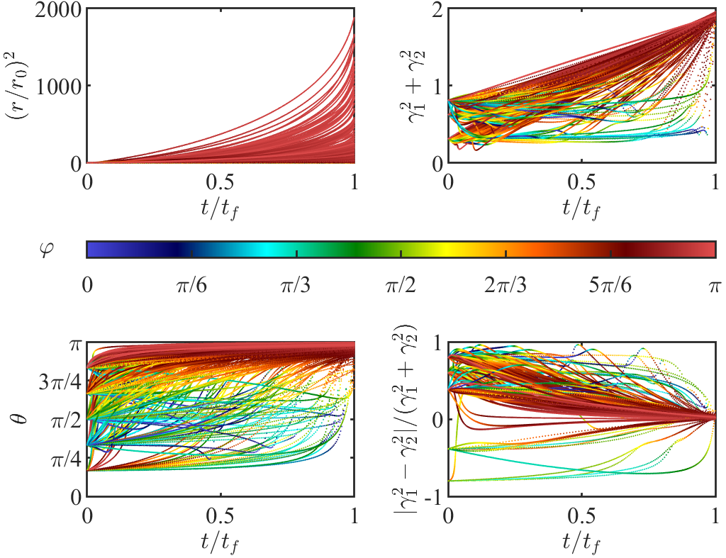
Figure 8: Time evolution of the distance $r$, the pinçons angles $\theta_{1}$, and $\theta_{2}$ (one line for each case), total intensity $\gamma_{1}^{2}+\gamma_{2}^{2}$ and anisotropy $(\gamma_{1}^{2}-\gamma_{2}^{2})/(\gamma_{1}^{2}+\gamma_{2}^{2})$ in the case expansion. (a) case of repelling dipolar expansion. (b) case of aligned expansion. The points are colored by the value of the pair mutual angle, $\varphi$.

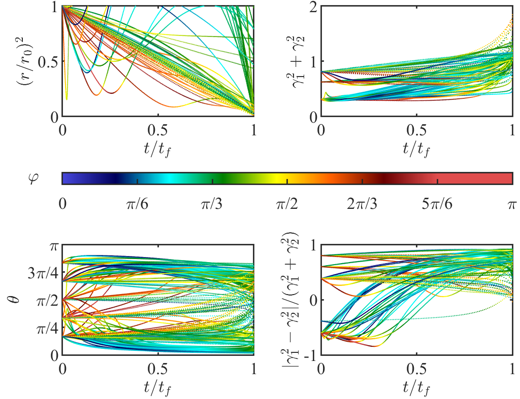
Figure 9: (a) Time evolution of the distance $r$, the pinçons angles $\theta_{1}$, and $\theta_{2}$ (one line for each case), total intensity $\gamma_{1}^{2}+\gamma_{2}^{2}$ and anisotropy $(\gamma_{1}^{2}-\gamma_{2}^{2})/(\gamma_{1}^{2}+\gamma_{2}^{2})$ in the case of explosive collapse. (b) Phase space for a pair of pinçons in the initial stage of the dynamics, just after pinçons creation. The phase space is $r$, $\gamma=\gamma_{1}^{2}+\gamma_{2}^{2}$ and $\xi=\xi(\theta_{1})\xi(\theta_{2})$. The points are colored by the value of the pair mutual angle $\varphi$ in all the figures.

Interestingly, the different cases partition in different areas the phase space $r$, $\gamma=\gamma_{1}^{2}+\gamma_{2}^{2}$ and $\xi=\xi(\theta_{1})\xi(\theta_{2})$, with $\xi(\theta)=\cos(\theta)\big{(}1-3\cos^{2}(\theta)\big{)}$, as illustrated in figure 9-b. One sees that the collapse mode tends to occur around $\xi=0$ meaning that at least one of the two pinçons tend to orientate at $\pi/2$, $\arccos(1/\sqrt{3})$ or $\pi-\arccos(1/\sqrt{3})$ from the separation vector. In contrast, the two expansion modes proceed with $\xi=\pm 2$, corresponding to situations where the pinçons are aligned or anti-aligned with their separation vector. Summarizing, we see that we observe two new cases with respect to the dipole dynamics, namely a new mode of expansion, made with two aligned dipole following each other, and a new mode of collapse following the law $\xi(\theta_{1})\xi(\theta_{2})=0$, with one component reaching the asymptotic value $\gamma=1$, and corresponding to a generic reconnection event. In the sequel, we study in more details these events.

III.4.2 Scaling laws of collapse

During the collapse stage, we fit the radius evolution with a power law in order to compare the exponent with the Leray scaling $\sqrt{t_{c}-t}$ Leray34 . Figure 10 (a) shows the histogram of the values of the exponent obtained by fitting the law $r(t)=\beta_{c}(t_{c}-t)^{\delta}$ for the collapse cases. We see that most of the values are near $1/2$ which correspond to the Leray exponent. Figure 10 (b) shows the time dynamics of rescaled squared radius. We see that the Leray scaling is verified asymptotically as $t/t_{c}\to 1$.

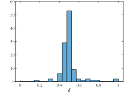
Figure 10: (a) Histogram of the values of the power law exponent $\delta$. (b) Squared distance rescaled by for the explosive collapse cases. The black dashed line correspond to the Leray scaling with $\delta=1/2$. We see that for $t/t_{c}$ close to $1$, most of the curves follow a power law with a power exponent $\delta$ close to $1/2$.

III.4.3 Full collapse dynamics

The full dynamics of reconnection events can be investigated using a patching between the short time behavior, and the large time behavior, allowing e.g. the turbulent stress to decay like $\exp(-t/\tau_{\text{forcing}})$, where $\tau_{\text{forcing}}$ is a time scale associated to large scales. As shown on Figure 11, for the same initial configuration, when dissipation is high and the forcing characteristic time is short, the pinçons die very fast with no close interaction. On the contrary, if the dissipation is too low with a forcing persistent enough, the dynamics is very similar to the case without dissipation, and the pinçons still collapse in a explosive manner with their intensities tending to 1. Two intermediate cases are found where we have a collapse stage followed by a separation stage without explosion. These typical examples are illustrated in figure 13 (a-b). In both cases, we observe first a collapse phase and then a separation phase although the particular dynamics are quite different. In the case of (a) where the dissipation and the forcing characteristic time are rather small, the transition between the two phases happens at a closer distance and has a configuration similar to the dipole with one of the pinçons axis abruptly turning from an angle close to 0 to an angle close to $\pi$, then the pinçons die very fast. In the case of (b) with larger dissipation and a more persistent forcing, the dynamics is smoother with hardly any change in the dipole relative orientation, only the axis angles change slowly and the pinçons survive a long time with a stable configuration. During the interaction, the maximum velocity and vorticity near the pair of pinçons shown on Figure 12 exhibit marked oscillations, due to the finite resolution of the grid. Using a moving average, we see however that for the cases where the intensities tend to 1, the maximum velocity and vorticity tend to infinity as expected. If we now look at the case of close interaction with a final separation corresponding to Figure 13 (a), they first decrease during the collapse stage until the time of minimum of $r$, after which they increase until the angle is close to $\phi=\pi$, then, they finally both decay to zero when separating. This behaviour is reminiscent of what is happening during a reconnection of vortex rings, where the distance between rings decay like $\sqrt{t_{c}-t}$, with maximum velocity and vorticity growing up then decaying yao2020 .

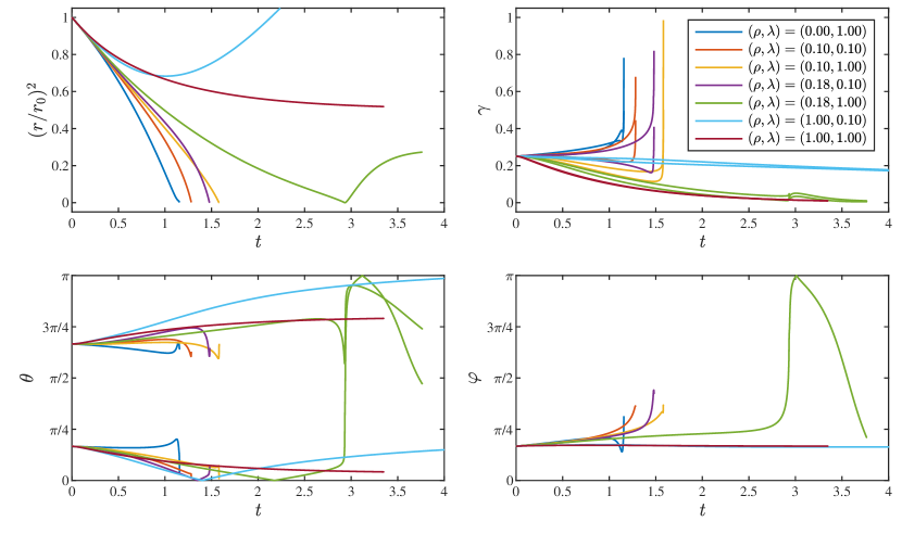
Figure 11: Time evolution of the different variables characterizing the pair of pinçons for 7 cases with the same initial configuration but with different forcing characteristic time coefficient $\lambda=\tau_{\nu}/\tau_{\text{forcing}}=r_{0}^{2}/(\nu\tau_{\text{forcing}})$ and dissipation coefficient $\rho=(\psi(0)/C_{\psi})(r_{0}/\eta)^{2}$. We see that on the one hand, when dissipation is high and the forcing time is short, the pinçons die very fast with no close interaction. On the other hand, if the dissipation is low, the dynamics is very similar to the case without dissipation, and the pinçons still collapse in a explosive manner with their intensities tending to 1. Two intermediate cases are found where we have both the collapse dynamics and a separation dynamics without explosion.

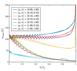
Figure 12: Time evolution of the maximum of velocity field (a) and vorticity field (b) around a pair of pinçons with same initial configurations and different forcing characteristic time coefficient $\lambda=\tau_{\nu}/\tau_{\text{forcing}}$ and dissipation coefficient $\rho$. The values correspond to a moving average over 15 time steps.

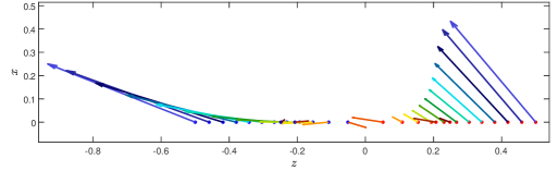
Figure 13: Dynamics of a pair of pinçons as a function of time for two different forcing characteristic time coefficient ($\lambda$) and dissipation coefficient $\rho$ : (a) $(\rho,\lambda)=(0.18,1.00)$ and (b) $(\rho,\lambda)=(1.00,0.10)$. The color of the vector codes the time, from $t=0$ (dark blue) to $t=t_{\text{final}}$ (dark red). In both cases, the two points of the pair (blue and red points) move initially towards each other and then their orientations change and they repulse each other. In the case of (a), the transition between the two phases has a configuration similar to the dipole with one of the pinçons axis abruptly turning from an angle close to 0 to an angle close to $\pi$, then the pinçons die very fast. In the case of (b), the dynamics is smoother with hardly any change in the dipole relative orientation, only the axis angles change slowly and the pinçons survive a long time with a stable configuration.

IV Discussion

We have introduced a model of singularities of Navier-Stokes, named pinçons , that are discrete particles characterized by their position and ”spin”. These particles follow a nontrivial dynamics, obtained by the condition that the coarse-grained velocity field around these singularities obeys locally Navier-Stokes equations. We have shown that this condition can only be satisfied provided the coarse-graining scale is of the order of the Kolmogorov scale.When immersed in a regular field, the pinçons are further transported and sheared by the regular field, experiencing a friction together with an energy injection coming from by Reynolds stress of the regular field. We have used these properties to devise a toy model of pinçon interactions, that can be either seen as a generalization of the vorton model of NovikovNovikov83 , that was derived for the Euler equations, or as an Ising model of Navier-Stokes singularities, that can be use to get insight on small scale behavior of Navier-Stokes equations. As an example, we have studied the properties of the interaction of two pinçons , at the early and late stage of their evolution, and in the presence or absence of a stochastic forcing induced by the possible Reynolds stress.

Quite interestingly, we have identified several modes of interactions at short times, that are characterized by the values of the parameter $\xi(\theta)=\cos(\theta)\big{(}1-3\cos^{2}(\theta)\big{)}$, where $\theta$ is the angle between the spin of the pinçon and the axis of the pair. Specifically, in the absence of noise, we identified two modes of expansion of the pair with $\xi=\pm 2$, corresponding to situations where the pinçon are aligned or anti-aligned with their separation vectors, and one mode of collapse with $\xi=0$. In the presence of noise, we observe and additional transient non-equilibrium steady state expansion mode, with $\xi=0$, and the pinçons are perpendicular to the axis of the pair. The quantity $1-3\cos^{2}(\theta)$ actually plays an important role in the theory of liquid crystals, as its average defines the order parameter of the system $s=(1-3\cos^{2}(\theta))/2$, with possible transitions between liquid ($s=0$) and nematic phase ($s=1$). The different interaction modes therefore open the way to interesting different collective behaviors when considering a larger collection of pinçons . Whether such behaviors are of relevance to the actual physics of turbulence is still an open issue, as the pinçon model ignores on a number of issues that may limit its range of validity: existence of large nonlocal energy transfer at the Kolmogorov scale, dilute approximation for the pinçon , scale separation between the pinçon and the ambiant large scale velocity field, to name but a few.

Our study of the interaction of two pinçon however already revealed some interesting similarities with reconnection between two vortex rings. Indeed, we observe that the collapse generally obeys a $\sqrt{t_{c}-t}$ that is observed during reconnection, and is characterized by transient growth of velocity or vorticity like in the reconnection. From another point of view, the pinçons dynamics is also reminiscent of the two fluid model of superfluid, where the ”regular” field, made of phonons, interact with the local topological defects that form the quantized vortices. However, as shown by Villois20 , the interaction of quantized vortices leads to Leray scaling, with distance between vortices decaying like $\sqrt{t_{c}-t}$. In a broader sense, the description of the interaction between pinçons and a regular field is parallel to the interaction of localized wave packets interacting with a mean flow, in the WKB-RDT model of Laval2004 . By analogy, one may then wonder whether it would be possible to use the pinçons as a subgrid scale model of turbulence, allowing to describe the interaction of a velocity field filtered at the Kolmogorov length, with a collection of pinçons that encode the very intense energy transfers that are observed when scanning very small scales of turbulence [S16]. If the pinçon model proved accurate enough to describe small scale turbulence, it would then enable the use of larger time-steps, as the motion of the small scale motions is governed by Lagrangian motions. Another issue is whether a short range regularization is needed at short distances to make the model applicable to subgrid modelling.

Even if the pinçon model does not accurately describe the behavior of small scale turbulence, it is is an out-of-equilibrium statistical model of Navier-Stokes singularities with many interaction modes, that bears some similarity with liquid crystal interactions. It may then stimulate new ideas regarding turbulence dynamics and properties and play a similar role than the Ising model in statistical mechanics.

This work has been funded by the ANR, project EXPLOIT, grant agreement no. ANR-16-CE06-0006-01.

We thank I. Dornic for useful discussions and J. Gibbon and Y. Pomeau for useful comments. The constructive remarks of two referees led to substantial enrichment of the model with respect to its original setting.

V Appendix

V.1 Useful properties

We introduce the function: $\phi(\textbf{x},\gamma)=\|\textbf{x}\|-\gamma\cdot\textbf{x}$. Such function has the properties:

$$\mbox{${\bf\nabla}$}_{\textbf{x}}\phi = \frac{\textbf{x}}{\|\textbf{x}\|}-\gamma$$ (39)

$$\phi = \textbf{x}\cdot\mbox{${\bf\nabla}$}_{\textbf{x}}\phi$$ (40)

$$\mbox{${\bf\nabla}$}_{\gamma}\phi = -\textbf{x}$$ (41)

$$\Delta_{\textbf{x}}(\ln(\phi)) = \frac{1-\gamma^{2}}{\phi^{2}}.$$ (42)

Therefore, $\textbf{v}_{\alpha}$ can also be written:

$$\textbf{v}_{\alpha}=-2\mbox{${\bf\nabla}$}(\ln\phi_{\alpha})+2\textbf{x}\Delta\ln(\phi_{\alpha}).$$ (43)

With such expression, it is easy to check that $\textbf{v}_{\alpha}$ is of zero divergence everywhere except at $x=0$, where it is undefined.

V.2 Computation of the generalized momentum

By definition:

$$\boldsymbol{\Pi}_{\alpha}=\frac{1}{4\pi}\oint_{S_{\textbf{x}_{\alpha}}}\textbf{v}_{\alpha}{dS},$$ (44)

where ${S_{\textbf{x}_{\alpha}}}$ is a sphere of center $\textbf{x}_{\alpha}$, and of radius unity, and the integration is perform only over the surface of the sphere. Taking spherical coordinate system with respect to a vertical axis along $\boldsymbol{\gamma}_{\alpha}$, $\textbf{x}-\textbf{x}_{\alpha}=(\cos\psi\sin\theta,\sin\psi\sin\theta,\cos\theta)$, it is easy to see that the azimutal average of $\textbf{x}-\textbf{x}_{\alpha}$ perpendicular to $\boldsymbol{\gamma}_{\alpha}$ is zero, and that the only nonzero component is along $\boldsymbol{\gamma}_{\alpha}$, and gives $\langle\textbf{x}-~{}\textbf{x}_{\alpha}\rangle_{\psi}=(0,0,\cos\theta)$. Using the fact that $\cos\theta=(1-\phi_{\alpha})/\gamma$ with $\gamma=\|\boldsymbol{\gamma}_{\alpha}\|$, we thus get the azimutal average of $\textbf{v}_{\alpha}$ as

$$\langle\textbf{v}_{\alpha}\rangle_{\psi} = (0,0,C);$$

$$C = \frac{2\gamma}{\phi}-\frac{2(1-\phi)}{\gamma\phi}+2\frac{(1-\gamma^{2})(1-\phi)}{\gamma\phi^{2}},$$

where we have dropped the subscripts $\alpha$ for simplicity. We may easily compute the integration of the various term over $\theta$ since after a change of variable $y=\cos\theta$, and we get for any $n\geq 0$

$$\langle\frac{1}{\phi^{n+1}}\rangle_{\theta} = \int\frac{\sin\theta}{\phi^{n+1}}d\theta;$$

$$= \int_{-1}^{1}\frac{dy}{(1-\gamma x)^{n+1}}$$

$$= \frac{1}{n\gamma}\left(\frac{1}{(1-\gamma)^{n}}-\frac{1}{(1+\gamma)^{n}}\right),$$

with the convention that $1/nx^{n}=\ln(x)$ when $n=0$. Summing all the terms, we finally obtain equation (9).

V.3 Velocity gradient tensor

$$\nabla\textbf{U} = \left(\frac{\partial U_{i}}{\partial x_{j}}\right)_{i,j}$$

$$= -\frac{2}{\phi}\left[\left(\boldsymbol{\gamma}-\frac{\textbf{x}}{\lVert\textbf{x}\rVert}+2\frac{(1-\gamma^{2})}{\phi}\textbf{x}\right)\otimes\frac{\nabla\phi}{\phi}+\left(\frac{1}{\lVert\textbf{x}\rVert}-\frac{1-\gamma^{2}}{\phi}\right)\mathbb{I}-\frac{\textbf{x}\otimes\textbf{x}}{\lVert\boldsymbol{x}\rVert^{3}}\right]$$

$$= -\frac{2}{\phi^{2}}\left[-\boldsymbol{\gamma}\otimes\boldsymbol{\gamma}+\frac{\left(3\gamma\mathrm{cos}(\theta)-\gamma^{2}(2+\mathrm{cos}^{2}(\theta))\right)}{(1-\gamma\,\mathrm{cos}(\theta))}\frac{\textbf{x}\otimes\textbf{x}}{\lVert\textbf{x}\rVert^{2}}+\frac{\boldsymbol{\gamma}\otimes\textbf{x}}{\lVert\textbf{x}\rVert}\right.$$

$$\left.-\frac{\left(\gamma\,\mathrm{cos}(\theta)+1-2\gamma^{2}\right)}{(1-\gamma\,\mathrm{cos}(\theta))}\frac{\textbf{x}\otimes\boldsymbol{\gamma}}{\lVert\textbf{x}\rVert}-\gamma\left(\mathrm{cos}(\theta)-\gamma\right)\mathbb{I}\right]$$

where $\mathrm{cos}(\theta)=(\boldsymbol{\gamma}\cdot\textbf{x})/(\gamma\lVert\textbf{x}\rVert)$

V.4 Vorton dynamics

The dynamics of the vortons is given by Novikov83 :

$$\dot{\textbf{x}}_{\alpha} = -\frac{1}{4\pi}\sum_{\beta\neq\alpha}\frac{\textbf{r}_{\alpha\beta}\times\boldsymbol{\gamma}_{\beta}}{\|\textbf{r}_{\alpha\beta}\|^{3}}$$ (45)

$$\dot{\boldsymbol{\gamma}}_{\alpha} = -\frac{1}{4\pi}\sum_{\beta\neq\alpha}\bigg{[}\frac{\boldsymbol{\gamma}_{\alpha}\times\boldsymbol{\gamma}_{\beta}}{\|\textbf{r}_{\alpha\beta}\|^{3}}-3\left(\boldsymbol{\gamma}_{\alpha}\cdot\textbf{r}_{\alpha\beta}\right)\frac{(\textbf{r}_{\alpha\beta}\times\boldsymbol{\gamma}_{\beta})}{\|\textbf{r}_{\alpha\beta}\|^{5}}\bigg{]}.$$ (46)

References

- (1) Novikov EA. 1983 Generalized dynamics of three-dimensional vortex singularities /vortons/. Zhurnal Eksperimentalnoi i Teoreticheskoi Fiziki 84, 975–981.
- (2) Leray J. 1934 Sur le mouvement d’un liquide visqueux emplissant l’espace. Acta Math. 63, 193248.
- (3) Gibbon JD, Pal N, Gupta A, Pandit R. 2016 Regularity criterion for solutions of the three-dimensional Cahn-Hilliard-Navier-Stokes equations and associated computations. Phys. Rev. E 94, 063103.
- (4) Constantin P, Weinan E, Titi ES. 1994 Onsager’s conjecture on the energy conservation for solutions of Euler’s equation. Communications in Mathematical Physics 165, 207–209.
- (5) Hicks W. 1899 Researches in vortex motion. Part III. On spiral or gyrostatic vortex aggregates. Proceedings of the Royal Society of London 62, 379387.
- (6) Constantin P, Majda A. 1988 The Beltrami spectrum for incompressible fluid flows. Communications in Mathematical Physics 115, 435–456.
- (7) Buckmaster T, De Lellis C, Székelyhidi L, Vicol V. 2018 Onsager’s Conjecture for Admissible Weak Solutions. Communications on Pure and Applied Mathematics 0.
- (8) Lundgren TS. 1982 Strained spiral vortex model for turbulent fine structure. The Physics of Fluids 25, 2193–2203.
- (9) Gilbert AD. 1993 A cascade interpretation of Lundgren stretched spiral vortex model for turbulent fine structure. Physics of Fluids A: Fluid Dynamics 5, 2831–2834.
- (10) Chorin AJ. 1991 Equilibrium statistics of a vortex filament with applications. Comm. Math. Phys. 141, 619–631.
- (11) Aksman MJ, Novikov EA, Orszag SA. 1985 Vorton Method in Three-Dimensional Hydrodynamics. Phys. Rev. Lett. 54, 2410–2413.
- (12) Alkemade AJQ, Nieuwstadt FTM, van Groesen E. 1993 The vorton method. Applied Scientific Research 51, 3–7.
- (13) Pedrizzetti G. 1992 Insight into singular vortex flows. Fluid Dynamics Research 10, 101–115.
- (14) Saffman PG, Meiron DI. 1986 Difficulties with three‐dimensional weak solutions for inviscid incompressible flow. The Physics of Fluids 29, 2373–2375.
- (15) Winckelmans G, Leonard A. 1988 Weak solutions of the three‐dimensional vorticity equation with vortex singularities. The Physics of Fluids 31, 1838–1839.
- (16) Greengard C, Thomann E. 1988 Singular vortex systems and weak solutions of the Euler equations. The Physics of Fluids 31, 2810–2813.
- (17) D.. G. 2021 Private communication. .
- (18) Yeung PK, Sreenivasan KR, Pope SB. 2018 Effects of finite spatial and temporal resolution in direct numerical simulations of incompressible isotropic turbulence. Phys. Rev. Fluids 3, 064603.
- (19) Dubrulle B. 2019 Beyond Kolmogorov cascades. Journal of Fluid Mechanics 867, P1.
- (20) Sverák V. 2011 On Landau’s solutions of the Navier–Stokes equations. Journal of Mathematical Sciences 179, 208.
- (21) Landau LD. 1944 A new exact solution of the Navier-Stokes equations. Dokl. Akad. Nauk SSSR 44, 311314.
- (22) Squire H. 1952 XCI. Some viscous fluid flow problems I: Jet emerging from a hole in a plane wall. The London, Edinburgh, and Dublin Philosophical Magazine and Journal of Science 43, 942–945.
- (23) Batchelor G. 2000 . In An introduction to Fluid Dynamics. Cambridge University Press.
- (24) Tian G, Xin Z. 1998 One-point singular solutions to the Navier-Stokes equations. Topol. Methods Nonlinear Anal. 11, 135–145.
- (25) Cannone M, Karch G. 2004 Smooth or singular solutions to the Navier–Stokes system ?. Journal of Differential Equations 197, 247–274.
- (26) Eyink GL. 2007-2008 Turbulence Theory. http://www.ams.jhu.edu/ eyink/Turbulence/notes/. course notes, The Johns Hopkins University,.
- (27) Kruskal MD. 1974 The Korteweg-de Vries equation and related evolution equations. In In: Nonlinear wave motion. (A75-14987 04-70) Providence pp. 61–83.
- (28) Calogero F. 1978 Motion of poles and zeros of special solutions of nonlinear and linear partial differential equations and related solvablemany-body problems. Il Nuovo Cimento B (1971-1996) 43, 177–241.
- (29) Calogero F. 2001 Classical many-body problems amenable to exact treatments. In Lecture Notes in Physics vol. 66. Springer Berlin.
- (30) Debue P, Valori V, Cuvier C, Daviaud F, Foucaut JM, Laval JP, Wiertel C, Padilla V, Dubrulle B. 2021 Three-dimensional analysis of precursors to non-viscous dissipation in an experimental turbulent flow. Journal of Fluid Mechanics 914, A9.
- (31) Nguyen F, Laval JP, Dubrulle B. 2020 Characterizing most irregular small-scale structures in turbulence using local Hölder exponents. Phys. Rev. E 102, 063105.
- (32) Kerr RM, Hussain F. 1989 Simulation of vortex reconnection. Physica D: Nonlinear Phenomena 37, 474–484.
- (33) Yao J, Hussain F. 2020a A physical model of turbulence cascade via vortex reconnection sequence and avalanche. Journal of Fluid Mechanics 883, A51.
- (34) Yao J, Hussain F. 2020b On singularity formation via viscous vortex reconnection. Journal of Fluid Mechanics 888, R2.
- (35) Kimura Y, Moffatt HK. 2018 A tent model of vortex reconnection under Biot–Savart evolution. Journal of Fluid Mechanics 834, R1.
- (36) Moffatt HK, Kimura Y. 2019a Towards a finite-time singularity of the Navier–Stokes equations Part 1. Derivation and analysis of dynamical system. Journal of Fluid Mechanics 861, 930–967.
- (37) Moffatt HK, Kimura Y. 2019b Towards a finite-time singularity of the Navier–Stokes equations. Part 2. Vortex reconnection and singularity evasion. Journal of Fluid Mechanics 870, R1.
- (38) Moffatt HK, Kimura Y. 2020 Towards a finite-time singularity of the Navier–Stokes equations. Part 2. Vortex reconnection and singularity evasion – CORRIGENDUM. Journal of Fluid Mechanics 887, E2.
- (39) Kimura Y, Moffatt HK. 2017 Scaling properties towards vortex reconnection under Biot–Savart evolution. Fluid Dynamics Research 50, 011409.
- (40) Villois A, Proment D, Krstulovic G. 2020 Irreversible Dynamics of Vortex Reconnections in Quantum Fluids. Phys. Rev. Lett. 125, 164501.
- (41) Yao J, Hussain F. 2020 On singularity formation via viscous vortexreconnection. Journal of Fluid Mechanics 888, R2.
- (42) Laval JP, Dubrulle B, Nazarenko S. 2004 Fast numerical simulations of 2D turbulence using a dynamic model for subfilter motions. Journal of Computational Physics 196, 184–207.