Robust Quantum Optimal Control with Trajectory Optimization

Abstract

The ability to engineer high-fidelity gates on quantum processors in the presence of systematic errors remains the primary barrier to achieving quantum advantage. Quantum optimal control methods have proven effective in experimentally realizing high-fidelity gates, but they require exquisite calibration to be performant. We apply robust trajectory optimization techniques to suppress gate errors arising from system parameter uncertainty. We propose a derivative-based approach that maintains computational efficiency by using forward-mode differentiation. Additionally, the effect of depolarization on a gate is typically modeled by integrating the Lindblad master equation, which is computationally expensive. We employ a computationally efficient model and utilize time-optimal control to achieve high-fidelity gates in the presence of depolarization. We apply these techniques to a fluxonium qubit and suppress simulated gate errors due to parameter uncertainty below $10^{-7}$ for static parameter deviations on the order of $1\%$.

I Introduction

Quantum optimal control (QOC) is a class of optimization algorithms for accurately and efficiently manipulating quantum systems. Early techniques were proposed for nuclear magnetic resonance experiments [1, 2, 3, 4, 5, 6, 7], and applications now include superconducting circuits [8, 9, 10, 11, 12, 13, 14, 15, 16, 17, 18, 19, 20, 21, 22, 23, 24], neutral atoms and ions [25, 26, 27, 28, 29, 30, 31, 32, 33, 34, 35, 36], nitrogen-vacancy centers in diamond [37, 38, 39, 40, 41, 42, 43], and Bose-Einstein condensates [44, 45, 46, 47]. In the context of quantum computation, optimal control is employed to achieve high-fidelity gates while adhering to experimental constraints. Experimental errors such as parameter drift, noise, and finite control resolution cause the system to deviate from the model used in optimization, hampering experimental performance [9, 14, 48, 33, 20]. Robust control improves upon standard optimal control by encoding model parameter uncertainties in optimization objectives, yielding performance guarantees over a range of parameter values [49, 50, 51]. We adapt robust control techniques from the robotics community to mitigate parameter-uncertainty errors for a superconducting fluxonium qubit.

Analytically-derived control pulses that mitigate parameter-uncertainty errors include composite pulses [52, 53, 54, 55], pulses designed by considering dynamic and geometric phases [56, 57], and pulses obtained with the DRAG scheme [58]. As compared to analytical techniques, QOC is advantageous for designing pulses that consider all experimental constraints and performance tradeoffs [17], and for constructing operations without a known analytic solution [9, 14]. Accordingly, recent work has sought to achieve robustness in QOC frameworks using closed-loop methods [59, 60, 61, 62] and open-loop methods [63, 64, 65, 20, 42, 66, 67, 3].

In this work, we study three open-loop robust control techniques that make the quantum state trajectory less sensitive to the uncertainties of static and time-dependent parameters:

1. A sampling method, similar to the work in Refs.  [65, 3, 20, 42].

2. An unscented sampling method [68, 69, 70] adapted from the unscented transform [71, 72] used in state estimation.

3. A derivative method, which penalizes the sensitivity of the quantum state trajectory to uncertain parameters.

We apply these techniques to the fluxonium qubit presented in [73]. We also show that QOC can solve important problems associated with fluxonium-based qubits: exploiting the dependence of $T_{1}$ on the controls to mitigate depolarization and synchronizing the phase of qubits with distinct frequencies. To ameliorate depolarization, we perform time-optimal control and employ an efficient depolarization model for which the computational cost is independent of the Hilbert space dimension. Leveraging recent advances in trajectory optimization within the field of robotics, we solve these optimization problems using ALTRO (Augmented Lagrangian TRajectory Optimizer) [74], which can enforce constraints on the control fields and the quantum state trajectory.

This paper is organized as follows. First, we describe ALTRO in the context of QOC in Sec. II. We outline realistic constraints for operating the fluxonium and define the associated QOC problem in Sec. III. Then, we formulate a method for suppressing depolarization in Sec. IV. Next, we describe three techniques for achieving robustness to static parameter uncertainties in Sec. V. We adapt the same techniques to mitigate 1/$f$ flux noise in Sec. VI.

II Background

In this section, we review the QOC problem statement and describe the ALTRO solver [74]. QOC concerns a vector $\mathbf{a}(t)$ of time-dependent control fields that steer the evolution of a quantum state $\ket{\psi(t)}$. The evolution of the state is governed by the time-dependent Schrödinger equation (TDSE),

$$i\hbar\frac{d}{dt}\ket{\psi(t)}=H(\mathbf{a}(t),t)\ket{\psi(t)}.$$ (1)

The Hamiltonian $H(\mathbf{a}(t),t)$ is determined by the quantum system and the external control fields. The QOC problem is to find the controls that minimize a functional $J[\mathbf{a}(t)]$, which we call the objective. To make the problem numerically tractable, the quantum state and controls are discretized into $N$ time steps, $\ket{\psi(t_{k})}\to\ket{\psi_{k}}$ and $\mathbf{a}(t_{k})\to\mathbf{a}_{k}$ where $t_{k}=t_{k-1}+\Delta t$ and $k\in\{1,...,N\}$. In the case of a single state-transfer problem, the objective is the infidelity of the time-evolved final state $\ket{\psi_{N}}$ and the intended target state $\ket{\psi_{T}}$, $J(\mathbf{a})=1-{\lvert\innerproduct{\psi_{T}}{\psi_{N}(\mathbf{a})}\rvert}^{2}$. Standard QOC solvers compute derivatives of the objective $\nabla J(\mathbf{a})$, which can easily be used to implement first-order optimization methods [75, 3, 17, 76].

Alternatively, the QOC problem can be formulated as a trajectory optimization problem and solved using specialized solvers developed by the robotics community [77, 78, 79, 74]. The objective $J(\mathbf{a})=\sum_{k}\ell_{k}(\mathbf{x}_{k},\mathbf{u}_{k})$ is expressed in terms of the cost function at each time step $\ell_{k}$, where $\mathbf{x}_{k}$ is the augmented state vector and $\mathbf{u}_{k}$ is the augmented control vector. We use the term augmented because these vectors contain all of the relevant variables in the optimization problem, not just the quantum state and the control fields, for an example see Sec. III. The augmented control contains all variables that the experimentalist may manipulate, and the augmented state contains all variables that depend on those in the augmented control. The variables in the augmented states depend on those in the augmented controls as defined by the differential equations governing the physical system, which are encoded in the discrete relation $\mathbf{x}_{k+1}=\mathbf{f}(\mathbf{x}_{k},\mathbf{u}_{k})$. For QOC, $\mathbf{f}(\mathbf{x}_{k},\mathbf{u}_{k})$ – which we call the discrete dynamics function – propagates the quantum state by integrating the TDSE (1) using a Runge-Kutta method [80] or an exponential integrator [81, 82, 83, 84].

We incorporate constraints on the augmented controls and states by formulating them as inequalities $\mathbf{g}_{k}(\mathbf{x}_{k},\mathbf{u}_{k})\leq\mathbf{0}$ or equalities $\mathbf{h}_{k}(\mathbf{x}_{k},\mathbf{u}_{k})=\mathbf{0}$. The constraint functions $\mathbf{g}_{k}$ and $\mathbf{h}_{k}$ may be vector-valued to encode multiple constraints, and equalities and inequalities are understood component-wise. To quantify constraint satisfaction, we define each constraint’s violation as the magnitude of its deviation: $\textrm{max}(g(\cdot),0)$ or $\absolutevalue{h(\cdot)}$, where $g$ and $h$ are components of constraint functions $\mathbf{g}_{k}$ and $\mathbf{h}_{k}$, respectively. Stated concisely, the trajectory optimization problem is: [2] x_1, …, x_N u_1, …, u_N - 1 ∑^N_k = 1ℓ_k (x_k,u_k), x_k+1 = f(x_k,u_k)  ∀ k g_k(x_k,u_k) ≤0  ∀ k h_k(x_k,u_k) = 0  ∀ k. We have formulated the problem such that the cost and constraint functions at time step $k$ may only depend on the augmented control and state at time step $k$. Although this structure may appear limiting, the problem can typically be reformulated to accomodate any cost or constraint function, for an example see Sec. III, and the ALTRO solver, which we introduce in the following discussion, exploits this structure to efficiently solve the problem.

Standard techniques for solving (II)-(II) typically fall into two categories: direct methods [85, 86] and indirect methods [87]. For indirect methods, the augmented controls are the decision variables, i.e., the variables the optimizer adjusts to solve the problem. The augmented states are obtained from the augmented controls using the discrete dynamics function, and they are used to evaluate derivatives of the cost functions. Then, the derivative information is employed to update the augmented controls. This approach is taken by standard QOC solvers such as GOAT [75], GRAPE [3, 17], and Krotov’s method [76]. Conversely, direct methods treat both the augmented controls and states as decision variables. In addition to minimizing the cost functions, the optimizer uses derivative information for the discrete dynamics function to satisfy the dynamics constraint (II) to a specified tolerance. In this sense, the TDSE (1) is a constraint that may be violated for intermediate steps of the optimization, where the quantum states need not be physical. The direct approach lends itself to a nonlinear program formulation, for which a variety of general-purpose solvers exist [88, 89].

Recent state-of-the-art solvers, such as ALTRO, combine the indirect and direct methods in a two-stage approach. First, ALTRO employs an indirect solving stage using the iterative linear-quadratic regulator (iLQR) algorithm [90] as the internal solver of an augmented Lagrangian method (ALM) [91, 92, 93]. In the second direct stage, ALTRO uses a projected Newton method [94, 95]. Next, we provide a more detailed summary of these two stages.

iLQR is an indirect method for minimizing the objective subject to the dynamics constraint, i.e., solving (II)-(II). First, iLQR uses an initial guess for the augmented controls to obtain the augmented states with the discrete dynamics function. iLQR then constructs quadratic models for each cost function using their zeroth-, first- and second-order derivatives in a Taylor expansion about the current augmented controls and states. These models are used with a recurrence relation between time steps to obtain the locally optimal update for the augmented controls. This recurrence relation is possible to derive in closed form because cost function contributions come only from the augmented control and state at a single time step [96]. Finally, a line search [97] is performed in the direction of the locally optimal update to ensure a decrease in the objective. This procedure is repeated until convergence is reached.

While indirect solvers like iLQR are computationally efficient and maintain high accuracy for the discrete dynamics throughout the optimization, they cannot handle nonlinear equality and inequality constraints (II)-(II). For QOC, a popular approach to handle such constraints is to add the constraint functions to the objective [14, 17, 20, 67]. However, this strategy does not guarantee that the constraints are satisfied as the solver trades minimization of the cost functions and constraint functions against each other. ALM remedies this issue by adaptively adjusting a Lagrange multiplier estimate for each constraint function to ensure the constraints are satisfied. ALM adds terms that are linear and quadratic in the constraint functions to the objective. Then, the new objective is minimized with iLQR. If the solution obtained with iLQR does not satisfy the constraints, the prefactors for the constraint terms in the objective are increased intelligently and the procedure is repeated.

ALM converges superlinearly, but poor numerical conditioning may lead to small decreases in the constraint violations near the locally optimal solution [98]. To address this shortcoming, ALTRO projects the solution from the ALM stage onto the constraint manifold using a (direct) projected Newton method, achieving ultra-low constraint violations $\sim 10^{-8}$. For more information on the details of the ALTRO solver, see Refs. [74, 99].

As opposed to standard QOC solvers, ALTRO can satisfy constraints on both the control fields and quantum states to tight tolerances. This advantage is crucial for this work, where multiple medium-priority cost functions are minimized subject to many high-priority constraints.

III QOC for the Fluxonium

In the following, we optimize quantum gates for the superconducting fluxonium qubit – a promising building block for quantum computers due to its high coherence times [100, 101, 102, 103, 104, 73]. In this section, we use the trajectory optimization formalism (II)-(II) to define the optimization problem (III)-(III), which we extend in subsequent sections to account for experimental error channels. To high accuracy, we approximate the fluxonium Hamiltonian near the flux-frustration point as a two-level system:

$$H/h =f_{q}\frac{\sigma_{z}}{2}+a(t)\frac{\sigma_{x}}{2}.$$ (2)

Here, $f_{q}$ is the qubit frequency at the flux-frustration point, $a(t)$ is the control governing the flux offset from the flux-frustration point, $h$ is Planck’s constant, and $\sigma_{z},\sigma_{x}$ are Pauli matrices. Although the coherent dynamics can be described with this two-level system model, our noise model, experimental constraints, and system parameters consider the full system, and they are representative of the fluxonium presented in [73].

First, we introduce the augmented control and state for the fluxonium gate problem. Since the ALTRO implementation we use does not currently support complex numbers, we represent the quantum states in the isomorphism $\mathcal{H}(\mathbb{C}^{n})\cong\mathcal{H}(\mathbb{R}^{2n})$ given in [17],

$$H\ket{\psi}\cong\begin{pmatrix}H_{\textrm{re}}&-H_{\textrm{im}}\\ H_{\textrm{im}}&H_{\textrm{re}}\end{pmatrix}\begin{pmatrix}\ket{\psi}_{\textrm{re}}\\ \ket{\psi}_{\textrm{im}}\end{pmatrix}.$$ (3)

We use $\psi$ – abandoning bra-ket notation – to denote the real representation of a state given by the right-hand-side of (3). To refer to the discrete moments of the flux, we introduce the notation $\int_{t}a_{k}\equiv\int^{t_{k}}_{t_{1}}a(t)\ \mathrm{d}t$, $a_{k}\equiv a(t_{k})$, $\mathrm{d}^{n}_{t}a_{k}\equiv\mathrm{d}^{n}a(t)/{\mathrm{d}t}^{n}\lvert_{t=t_{k}}$. The augmented control and state are:

$$\mathbf{u}_{k}=\begin{pmatrix}\mathrm{d}^{2}_{t}a_{k}\end{pmatrix},\quad\mathbf{x}_{k}=\begin{pmatrix}\psi^{0}_{k}\\ \psi^{1}_{k}\\ \int_{t}a_{k}\\ a_{k}\\ \mathrm{d}_{t}a_{k}\end{pmatrix}.$$ (4)

Here, the superscript on the quantum states $i\in\{0,1\}$ acts as a label. In standard QOC frameworks, the derivatives of the control fields are obtained with finite difference methods, e.g., $\mathrm{d}_{t}a_{k}\approx(a_{k+1}-a_{k})/\Delta t$ [17]. Because ALTRO requires that cost functions do not use information from multiple time steps, we make $\mathrm{d}^{2}_{t}a_{k}$ a decision variable and numerically integrate coupled ODEs to obtain $\mathrm{d}_{t}a_{k}$, $a_{k}$, and $\int_{t}a_{k}$ so that we may penalize them in cost functions. Similarly, the quantum states are obtained by numerically integrating the TDSE (1) with the fluxonium Hamiltonian (2) and the given flux $a_{k}$. These numerical integration rules are implemented in the discrete dynamics function for the problem, and they give rise to the dynamics constraint (III).

Next, we outline the constraints for this problem. Casting this problem in terms of a multi-state transfer problem, we fix as the initial states $\ket*{\psi^{0}_{1}}=\ket*{0}$, $\ket*{\psi^{1}_{1}}=\ket*{1}$ (III). The states at the final time step are constrained to be the target states $\ket*{\psi^{i}_{N}}=\ket*{\psi^{i}_{T}}\equiv U\ket*{\psi^{i}_{1}}\ \forall\ i$ (III) where $U=X/2,Y/2,Z/2$ denotes the target gate. Furthermore, we impose the normalization constraint ${\lvert\innerproduct*{\psi^{i}_{k}}{\psi^{i}_{k}}\rvert}^{2}=1\ \forall\ i,k$ (III) to ensure the solver does not take advantage of discretization errors in numerical integration. For the flux, we have the initial condition $\int_{t}a_{1}=\mathrm{d}_{t}a_{1}=0$ (III). We also enforce the boundary condition $a_{1}=a_{N}=0$ (III), (III) so the gates may be concatenated arbitrarily. We impose the zero net-flux constraint $\int_{t}a_{N}=0$ (III) which mitigates the inductive drift ubiquitous in flux-bias lines [105, 106, 73]. Additionally, the flux is constrained by $\lvert a_{k}\rvert\leq 0.5\ \textrm{GHz}\ \forall\ k$ (III) to ensure the two-level approximation remains valid (2). Above $0.5$ GHz, the relationship between the energy levels and the flux becomes strongly non-linear. All gates presented in this work satisfy these constraints to a maximum violation of $\sim 10^{-8}$.

The cost function at each time step is $\ell_{k}(\mathbf{x}_{k},\mathbf{u}_{k})=(\mathbf{x}_{k}-\mathbf{x}_{T})^{T}Q_{k}(\mathbf{x}_{k}-\mathbf{x}_{T})+\mathbf{u}^{T}_{k}R_{k}\mathbf{u}_{k}$ where $Q_{k}$ and $R_{k}$ are diagonal matrices of hyperparameters that assign weights to cost function contributions. The $Q_{k}$ term penalizes deviations from the target augmented state $\mathbf{x}_{T}=(\psi^{0}_{T},\psi^{1}_{T},0,0,0)^{T}$, which is consistent with the constraints we have imposed on $\ket*{\psi^{i}_{N}}$, $\int_{t}a_{N}$, and $a_{N}$. Accordingly, this term penalizes the squared difference of $\psi^{i}_{k}$ and $\psi^{i}_{T}$ and penalizes the norm of $\int_{t}a_{k}$, $a_{k}$, and $\mathrm{d}_{t}a_{k}$. We penalize the squared difference of the final and target quantum states, rather than their infidelities, because the Hessian of the squared-difference cost function is diagonal – which makes matrix multiplications fast – and we wish to optimize $Z/2$ gates, which requires a metric that is sensitive to global phases for the initial states $\ket*{0}$ and $\ket*{1}$. Additionally, the $R_{k}$ term penalizes the norm of $\mathrm{d}^{2}_{t}a_{k}$. Penalizing the norm of $\mathrm{d}^{2}_{t}a_{k}$ and $\mathrm{d}_{t}a_{k}$ makes $a_{k}$ smooth, which mitigates high-frequency AWG transitions. Stated succinctly, the optimization problem takes the form: [2] x_1,…,x_N u_1,…,u_N-1 ∑_k=1^N (x_k-x_T)^T Q_k (x_k-x_T) + ∑_k=1^N-1 u_k^T R_k u_k x_k+1= f(x_k, u_k)  ∀ k —ψ^0_1⟩ = —0⟩, —ψ^1_1⟩ = —1⟩ ∫t a_1 = a_1 = d_t a_1 = 0 —ψ^i_N⟩ = —ψ^i_T⟩  ∀  i ∫t a_N = a_N = 0 |⟨ψ^i_k—ψ^i_k⟩ |^2 = 1  ∀ i, k —a_k— ≤0.5  GHz  ∀ k.

Next, we remark on our problem formulation. We put a cost function at all time steps because it benefits the iLQR solving stage [99]; although this may incentivize early achievement of the desired gate, as in Ref. [17], we are primarily concerned with achieving the gate at the final time step, which the target-state constraint (III) ensures. Additionally, the target-state constraint requires the final state to match the target state, including its global phase, up to our chosen maximum constraint violation $\sim 10^{-8}$. If we did not impose this constraint, the optimizer would be allowed to sacrifice the closed-system gate error to achieve better performance on the other cost functions, which is undesirable. To enforce a constraint in standard QOC frameworks, the prefactor for the constraint function is manually increased between separate optimization instances until the constraint is satisfied [14, 17, 20], which becomes infeasible for more than one constraint. ALM automates these prefactor updates to find a solution that satisfies all of the given constraints. Hence, ALTRO’s ability to handle multiple constraints makes it an attractive solver for QOC problems.

In extraordinarily difficult cases of QOC, it may be impossible to obey the physics of the system and achieve the desired gate [8], i.e., the dynamics constraint (III) and the target-state constraint (III) may be mutually unsatisfiable. In this case, the prefactors for the constraint function terms in the ALM objective will tend to infinity – leading to numerical instability – and the optimization will not converge. To maintain a constrained approach in this situation, the maximum constraint violation for the target-state constraint can be raised to a level commensurate with the minimum acceptable gate error.

Finally, for ALTRO’s first indirect stage, the augmented states are obtained explicitly with the discrete dynamics function, so the dynamics constraint and initial conditions (III)-(III) are satisfied by construction. In this stage, the rest of the constraint functions (III)-(III) are added to the objective in their isomorphism-equivalent form (3). Conversely, for the second direct stage, all of the constraints (III)-(III) are used to define the projection onto the constraint manifold, and the objective is unmodified. Hence, the quantum states become free parameters that are adjusted to satisfy the TDSE. Although the final solution’s deviation from the TDSE is never more than the maximum constraint violation, we explicitly integrate the TDSE when reporting gate errors to ensure accuracy. Exploring the benefit of direct optimization approaches for QOC is an interesting direction for future work.

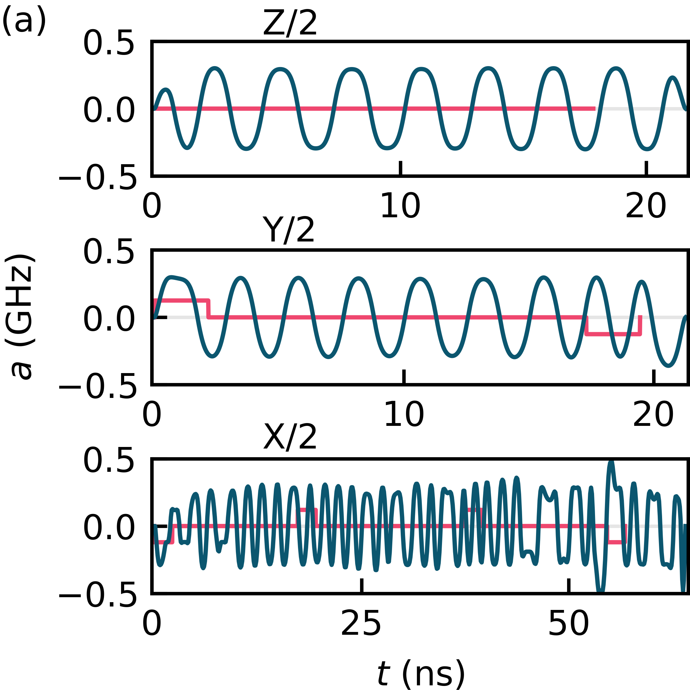
(a)

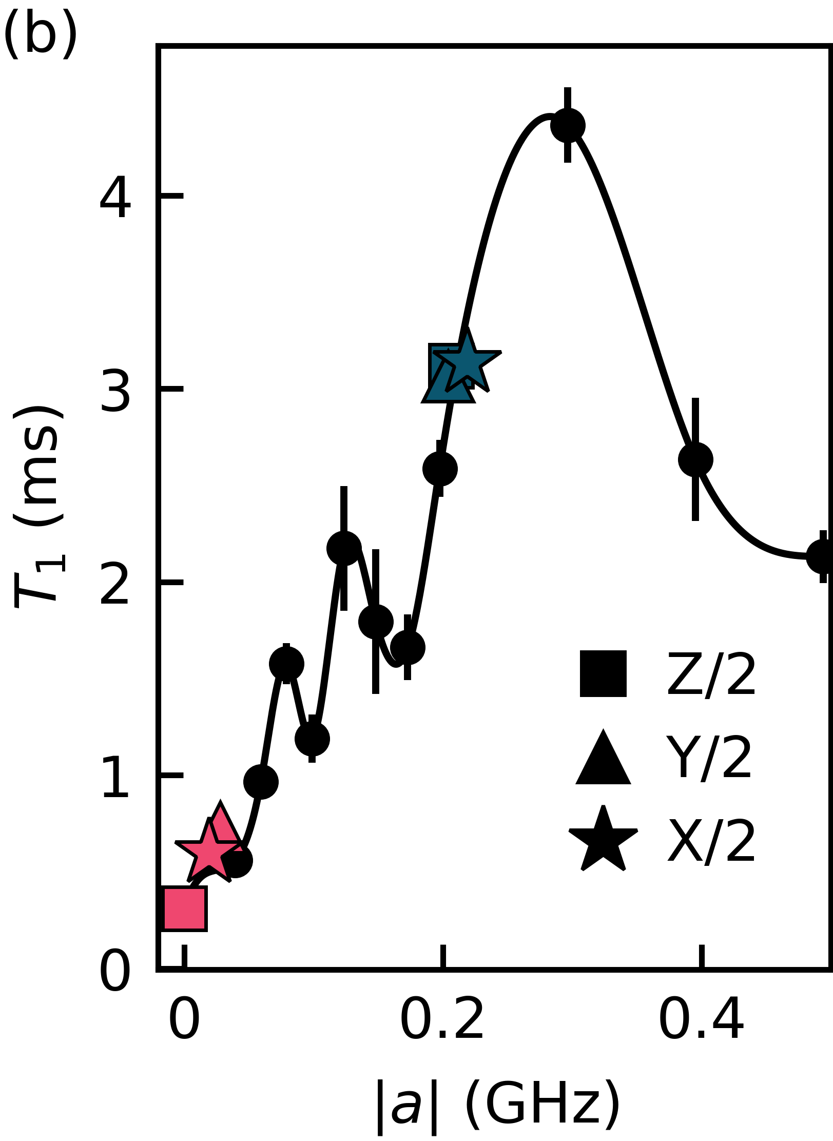
(b)

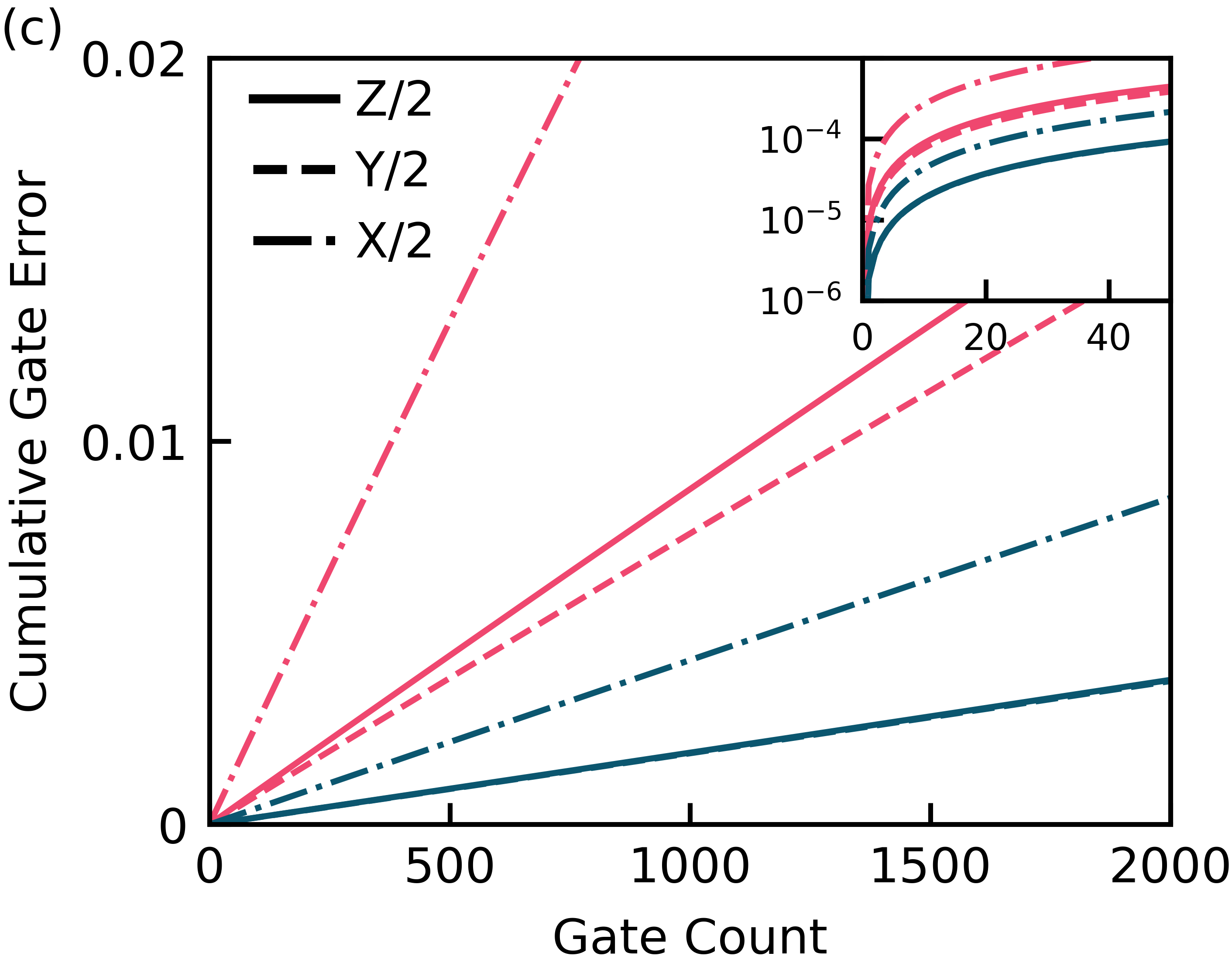
(c)

FIG. 1: (a) Flux pulses for the numerical gates (dark blue) and the analytic gates (light pink). (b) $T_{1}$ interpolation function used in optimization. Circle markers indicate measured $T_{1}$ times. Non-circle markers are plotted at the time-averaged absolute flux and the time-averaged $T_{1}$ time for each pulse. (c) Cumulative gate errors due to depolarization as a function of the number of gates applied. Cumulative gate errors for the numerical $Z/2$ and $Y/2$ gates are indistinguishable. Inset shows log-scaled cumulative gate errors for small gate counts.

IV Depolarization Mitigation

In this section, we outline a method for optimizing the flux to mitigate depolarization. For many superconducting circuits, the depolarization time $T_{1}$ is independent of the control parameters, so the fastest possible gate incurs the least depolarization error [107]. For the fluxonium, however, $T_{1}$ is strongly dependent on the flux. We enable the optimizer to trade longer gate times for longer $T_{1}$ times, or shorter $T_{1}$ times for shorter gate times, by making the gate time a decision variable. Additionally, previous work has modeled the gate error due to depolarization by evolving density matrices under a master equation [42, 107], or evolving a large number of states in a quantum trajectory approach [108]. We avoid the increase in computational complexity required for these techniques by penalizing the integrated depolarization rate in optimization.

The integrated depolarization rate is given by,

$$D_{1}(t)=\int_{0}^{t}T_{1}^{-1}[a(t^{\prime})]dt^{\prime}.$$ (5)

For the gates we consider here, where the gate time is small compared to $T_{1}$, the integrated depolarization rate is proportional to the probability of a depolarization event. Additionally, the integrated depolarization rate is a reasonable proxy for the gate error incurred because depolarization errors are incoherent – they increase monotonically in time without interference. The integrated depolarization rate is appended to the augmented state (4) and its norm is penalized in the $Q_{k}$ term of the objective by setting the corresponding element of the target augmented state to zero, see (III). $T_{1}$ as a function of the flux is obtained by evaluating a spline fit to experimental data, see Fig. 1(b).

Alternatively, modeling the depolarization with a master equation approach would require adding density matrices of size $n\times n$ to the augmented state, and a quantum trajectory approach would require adding many states of size $n$ to the augmented state, where $n$ is the dimension of the Hilbert space. By contrast, the integrated depolarization rate is a single real number; thus, the computational complexity of evaluating this depolarization model does not scale with the dimension of the Hilbert space.

To perform time-optimal control, we make the duration between time steps a decision variable [74]. The square root of the duration $\sqrt{\Delta t_{k}}$ is appended to the augmented control (4) and its square $\lvert\Delta t_{k}\rvert$ is used for integration in the discrete dynamics function. Although we constrain the bounds of the duration between reasonable positive values to maintain numerical stability, the optimizer may assign negative values to the duration for intermediate optimization iterations, so this squaring approach maintains positivity.

We analyze the effect of depolarization on the $X/2$, $Y/2$, and $Z/2$ gates obtained with our numerical method and the corresponding analytic gates presented in [73]. We use the Lindblad master equation to simulate $T_{1}$ dissipation for successive gate applications, and compute the cumulative gate error after each application, see Appendix A. The gate error reported in this text is the infidelity of the evolved state and the target state averaged over 1000 pseudo-randomly generated initial states.

The flux pulses for the numerical gates are approximately periodic with amplitudes $\sim 0.2\textrm{GHz}$, see Fig. 1(a). They are reminiscent of the analytically determined Floquet operations for a fluxonium described in [109] and realized in [110]. The numerical gate times are greater than the analytic gate times, but the numerical flux pulses spend more time at larger flux values, achieving higher $T_{1}$ times on average, see Fig. 1(b). The single-gate errors for both the analytic and numerical gates are less than $10^{-4}$, which makes them sufficient for quantum error correction – a prerequisite for fault-tolerant quantum computing [111, 112, 113]. However, the numerical gates achieve single-gate errors $\sim 5$ times less than those for the analytic gates, which tracks closely with their relative improvement on the integrated depolarization rate metric, see Appendix A. This advantage in single-gate errors corresponds to a significant reduction in error correction resources [114, 115]. Furthermore, for successive gate applications, the gate error due to depolarization is approximately linear in the gate count, which we expect for $t\ll T_{1}$, see Fig. 1(c). The gate error reduction for large gate counts is important for noisy, intermediate-scale quantum (NISQ) applications. These improvements are significant given the constraints we have imposed on the gates, and do not represent a fundamental limit to the optimization methods we have employed.

V Robustness to Static Parameter Uncertainty

We have formulated the QOC problem as an open-loop optimization problem, i.e., we do not incorporate feedback from the experiment into the optimization. However, the precise device parameters will deviate from the parameters we use in optimization, leading to poor experimental performance. We combat errors of this form using robust control techniques, making the state evolution insensitive to parameter uncertainty. As an example, we mitigate errors arising from the drift and finite measurement precision of the qubit frequency, which modifies the fluxonium Hamiltonian (2) by $f_{q}\rightarrow f_{q}+\delta f_{q}$. We consider three robust control techniques to accomplish this task: a sampling method, an unscented sampling method, and a derivative method.

V.1 Sampling Method

The sampling method incentivizes the optimizer to ensure that multiple copies of a state, each evolving with a distinct value of the uncertain parameter, achieve the same target state. Variants of this technique have been proposed in the context of QOC [65, 3, 20, 42]. For each initial state, we add two sample states $\ket*{\psi^{\pm}}$ to the augmented state (4). The discrete dynamics function is modified so the sample states evolve under the fluxonium Hamiltonian (2) with $f_{q}\rightarrow f_{q}\pm\sigma_{f_{q}}$ for a fixed standard deviation $\sigma_{f_{q}}$ of the qubit frequency, acting as a hyperparameter. We penalize the infidelities of the sample states with respect to the target state by adding a cost function to the objective of the form $\sum_{k,\pm}b_{k}(1-{\lvert\innerproduct*{\psi_{T}}{\psi^{\pm}_{k}}\rvert}^{2})$ where $b_{k}$ is a constant we supply. For this method, the standard orthonormal basis states are an insufficient choice for the initial states. As an example, a $Z/2$ gate achieved by idling at the flux frustration point ($a_{k}=0\ \forall\ k$) will be robust to qubit frequency detunings for the initial states $\ket{0}$ or $\ket{1}$ because the infidelity metric is insensitive to global phases, but this gate will not be robust for any other initial states. Therefore, we choose the four initial states $\{\ket{0},\ket{1},(\ket{0}+i\ket{1})/\sqrt{2},(\ket{0}-\ket{1})/\sqrt{2}\}$ [116], whose outer products span the operators on the Hilbert space, and we refer to them as the operator basis.

V.2 Unscented Sampling Method

Whereas the sampling method penalizes the deviations of the sample states from the target state, the unscented sampling method penalizes the deviations of the sample states from the nominal state [68, 69, 70]. Accordingly, the cost function we add to the objective takes the form $\sum_{k,j}c_{k}(\psi^{j}_{k}-\psi_{k})^{T}(\psi^{j}_{k}-\psi_{k})$, where $c_{k}$ is a constant we supply, $\psi_{k}$ is the evolved initial state (nominal state), and $\psi^{j}_{k}$ is a sample state that evolves under a modified Hamiltonian similar to that in the sampling method. The sample states are chosen to encode a unimodal distribution over the $2n$ elements of the nominal state, modeling the uncertainty in the state as a result of the uncertainty in the parameter. We use the unscented transform [71, 72] to accurately propagate the mean and covariance of this distribution between time steps, or equivalently, through the transformation of the TDSE (1). Unlike the sampling method, the cost function for the unscented sampling method is sensitive to global phases. Accordingly, we do not observe a performance increase when using more than one initial state. A detailed procedure for the unscented transformation is given in Appendix B.

V.3 Derivative Method

The derivative method penalizes the sensitivity of the state to the uncertain parameter, which is encoded in the $l$^th-order state derivative $\ket*{\partial_{f_{q}}^{l}\psi}\equiv\partial_{f_{q}}^{l}\ket*{\psi}$. In the $m$^th-order derivative method, we append all state derivatives of order $1,\dots,m$ to the augmented state (4) for each initial state. We obtain the state derivatives at each time step by performing forward-mode differentiation on the TDSE (1). For example, the dynamics for the $1$^st-order derivative method are:

$$i\hbar\frac{d}{dt}\ket{\psi} =H\ket{\psi},$$ (6)

$$i\hbar\frac{d}{dt}\ket{\partial_{f_{q}}\psi} =H\ket{\partial_{f_{q}}\psi}+(\partial_{f_{q}}H)\ket{\psi}.$$ (7)

We integrate the coupled ODEs with exponential integrators, see Appendix C. While the state $\ket*{\psi}$ has unit norm, the state derivatives $\ket*{\partial^{l}_{f_{q}}\psi}$ need not, as is evident from the non-unitary dynamics (7). We penalize the norms of the isomorphism-equivalent state derivatives in the $Q_{k}$ term of the objective by setting the corresponding elements of the target augmented state to zero, see (III). Intuitively, this corresponds to penalizing the sensitivity of each state element to the uncertain parameter. As was the case for the unscented sampling method, we do not observe a performance increase when using more than one initial state for the derivative method. We present the runtimes of our implementations of the three robust control methods in Appendix D.

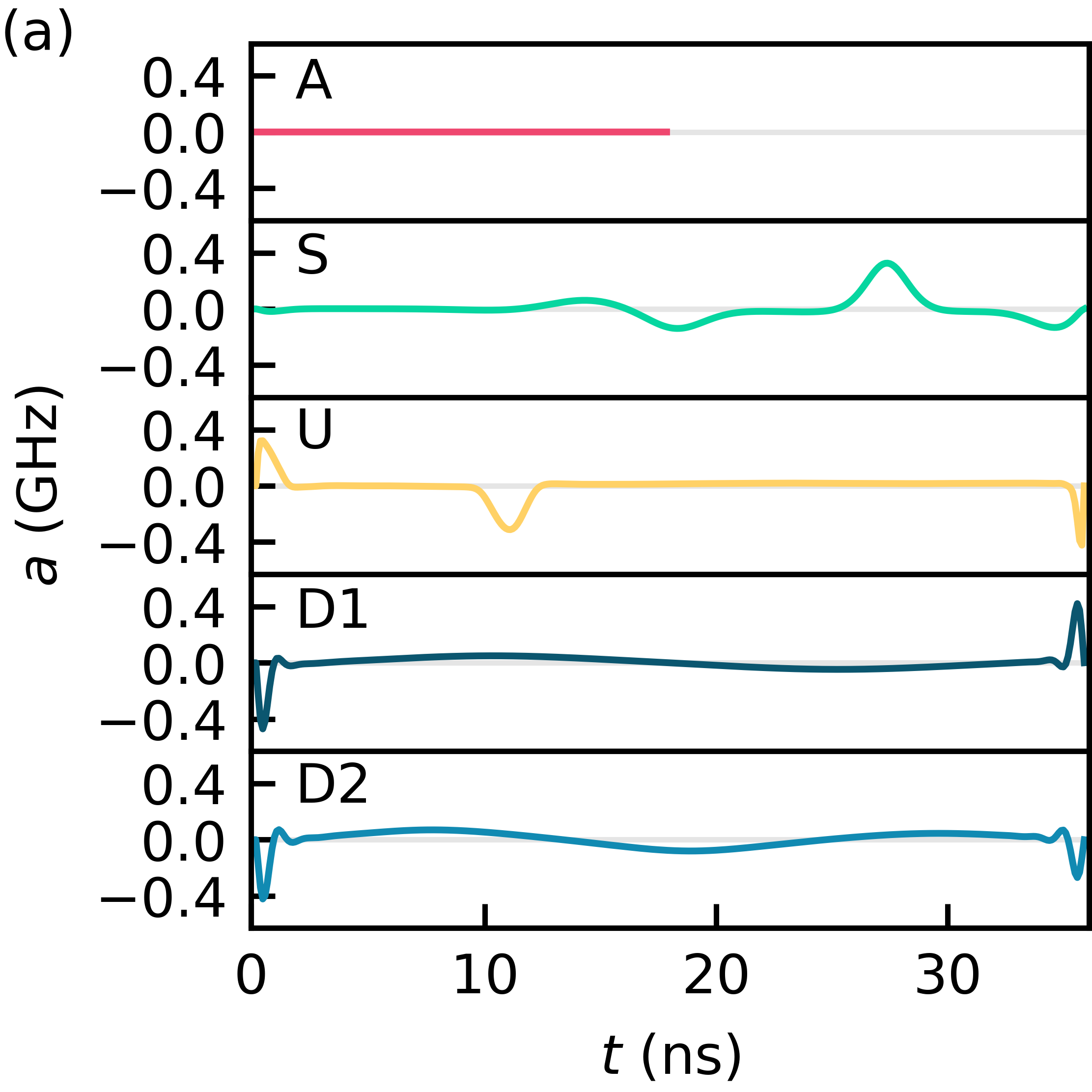
(a)

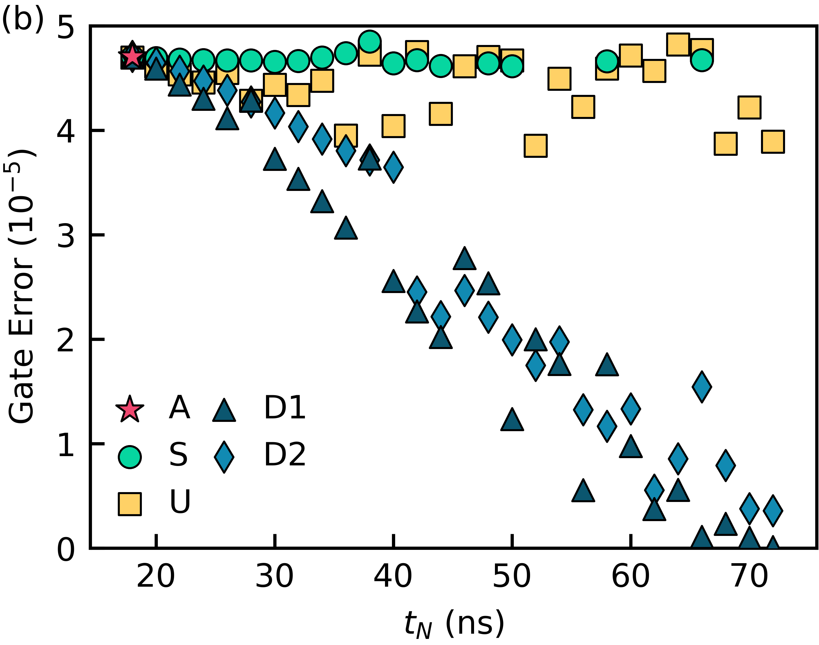
(b)

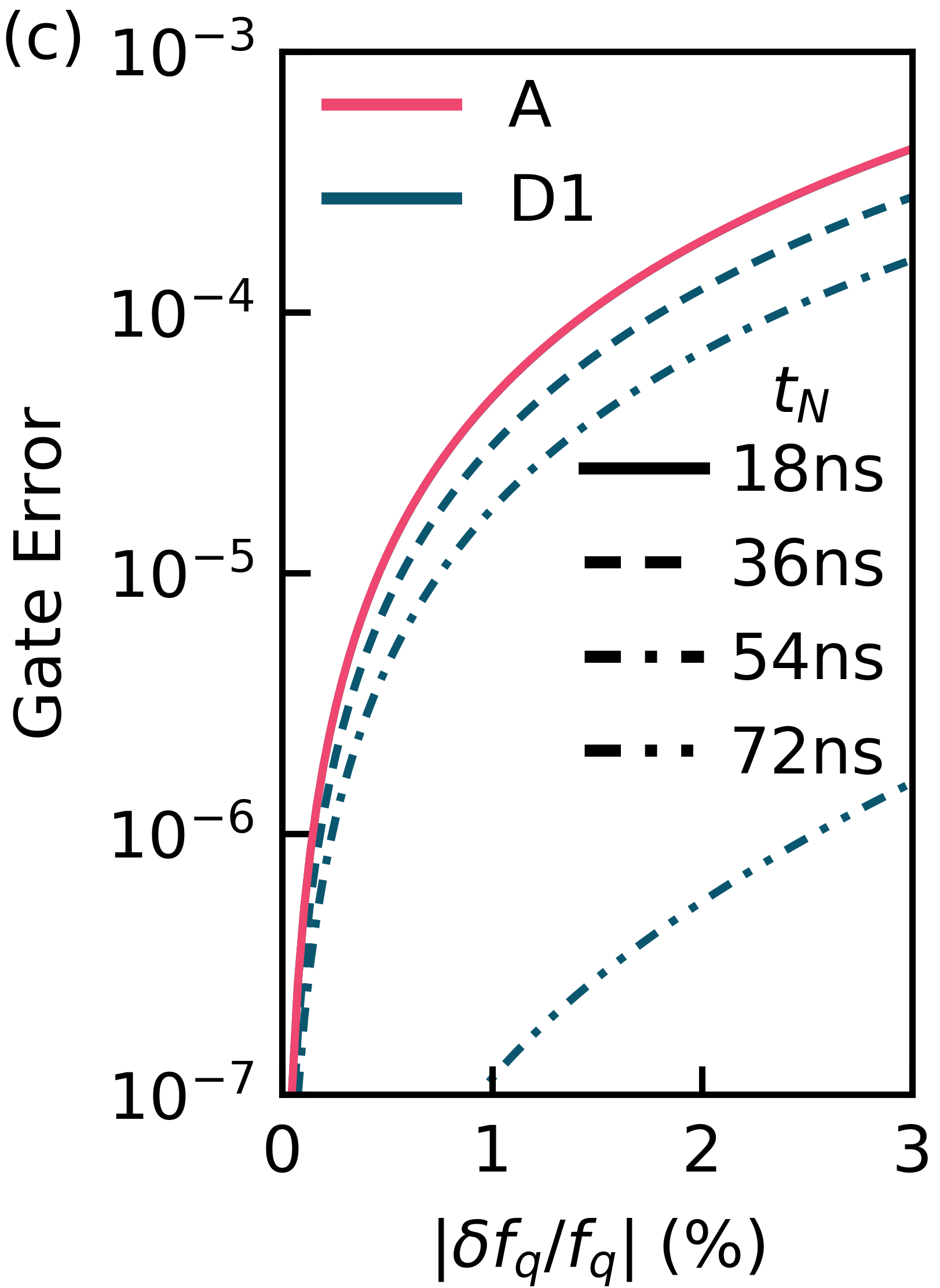
(c)

FIG. 2: (a) Flux pulses for $Z/2$ gates robust to qubit frequency detunings constructed with the analytic (A), sampling (S), unscented sampling (U), and the 1^st- and 2^nd-order derivative methods (D1, D2). The flux pulses shown for the sampling, unscented sampling, and derivative methods are optimized for twice the gate time of the analytic gate. (b) Single-gate error at a one-percent qubit frequency detuning as a function of the gate time. Missing data points represent gates with a gate error greater than $5\cdot 10^{-5}$. (c) Single-gate error as a function of the qubit frequency detuning. The gate errors for the analytic and 1^st-order derivative methods are shown for gate times which are multiples of $1/4f_{q}\sim 18\textrm{ns}$. The gate errors for the two methods are indistinguishable at the gate time $18\textrm{ns}$.

V.4 Comparison

We examine the gate errors due to a static qubit frequency detuning for the $Z/2$ gates obtained with the robust control techniques and the analytic $Z/2$ gate. To compute the gate error, an initial state is evolved under the fluxonium Hamiltonian (2) two separate times with the transformations $f_{q}\rightarrow f_{q}\pm\delta f_{q}$ at the stated qubit frequency detuning $\delta f_{q}$. The reported gate error is the infidelity of the evolved state and the target state averaged over the two transformations for each of $1000$ pseudorandomly generated initial states. We set $\sigma_{f_{q}}/f_{q}=1\%$ for the sampling and unscented sampling methods.

The analytic gate corresponds to idling at the flux frustration point $a_{k}=0\ \forall\ k$, see Fig. 2(a). Its gate time $1/4f_{q}\sim 18\textrm{ns}$ is the shortest possible for a $Z/2$ gate on the device. The gate’s erroneous rotation angle $2\pi\delta f_{q}/4f_{q}$ is linear in the qubit frequency detuning, resulting in a gate error that is quadratic in the detuning. At a one-percent detuning $\lvert\delta f_{q}/f_{q}\rvert=1\%$, the gate error is $\sim 4.7\cdot 10^{-5}$, which is sufficient for quantum error correction.

For the sampling method, the gate error at a one-percent qubit frequency detuning does not decrease substantially over the range of gate times, and begins to increase above $5\cdot 10^{-5}$ for gate times greater than $\sim 50$ns, see Fig. 2(b). Optimization results for the sampling method reveal that it is typically able to achieve a high fidelity for one sample $\ket{\psi^{\pm}}$, but not the other $\ket{\psi^{\mp}}$, indicating that it is difficult for the optimizer to make progress on both objectives. For the unscented sampling method, the gate error at a one-percent detuning does not decrease substantially over the gate times, but it does reach a minimum of $\sim 3.9\cdot 10^{-5}$ near fractions of the Larmor period: $2/4f_{q}\sim 36\textrm{ns}$, $3/4f_{q}\sim 54\textrm{ns}$, and $4/4f_{q}\sim 72\textrm{ns}$.

The two derivative methods converge on qualitatively similar flux pulses that idle near the flux frustration point and use fast triangle movements at the boundaries, similar to the flux pulse produced by the unscented sampling method. For both derivative methods, the gate error at a one-percent qubit frequency detuning decreases super-linearly in the gate time. For the 1^st-order method, the gate error at a one-percent detuning reaches $10^{-7}$ at the Larmor period $1/f_{q}\sim 72$ns, see Fig. 2(c). This result mimics the ability of composite pulses to mitigate parameter uncertainty errors to arbitrary order with sufficiently many pulses [55]. It is difficult to choose an appropriate composite pulse for the problem studied here due to our Hamiltonian and experimental constraints. A comparison between composite pulses and numerical techniques could be an interesting topic for future study.

Furthermore, the ability to perform $Z$-type gates in any given time is critical for synchronizing phases in multi-qubit experiments, where the qubits have distinct frequencies. Notably, the analytic gate studied here cannot be extended to gate times other than $1/4f_{q}$. We can find gates using the numerical methods at all gate times at and above $1/4f_{q}$, see Fig. 2(b). These numerical methods offer an effective scheme for synchronizing multi-qubit experiments.

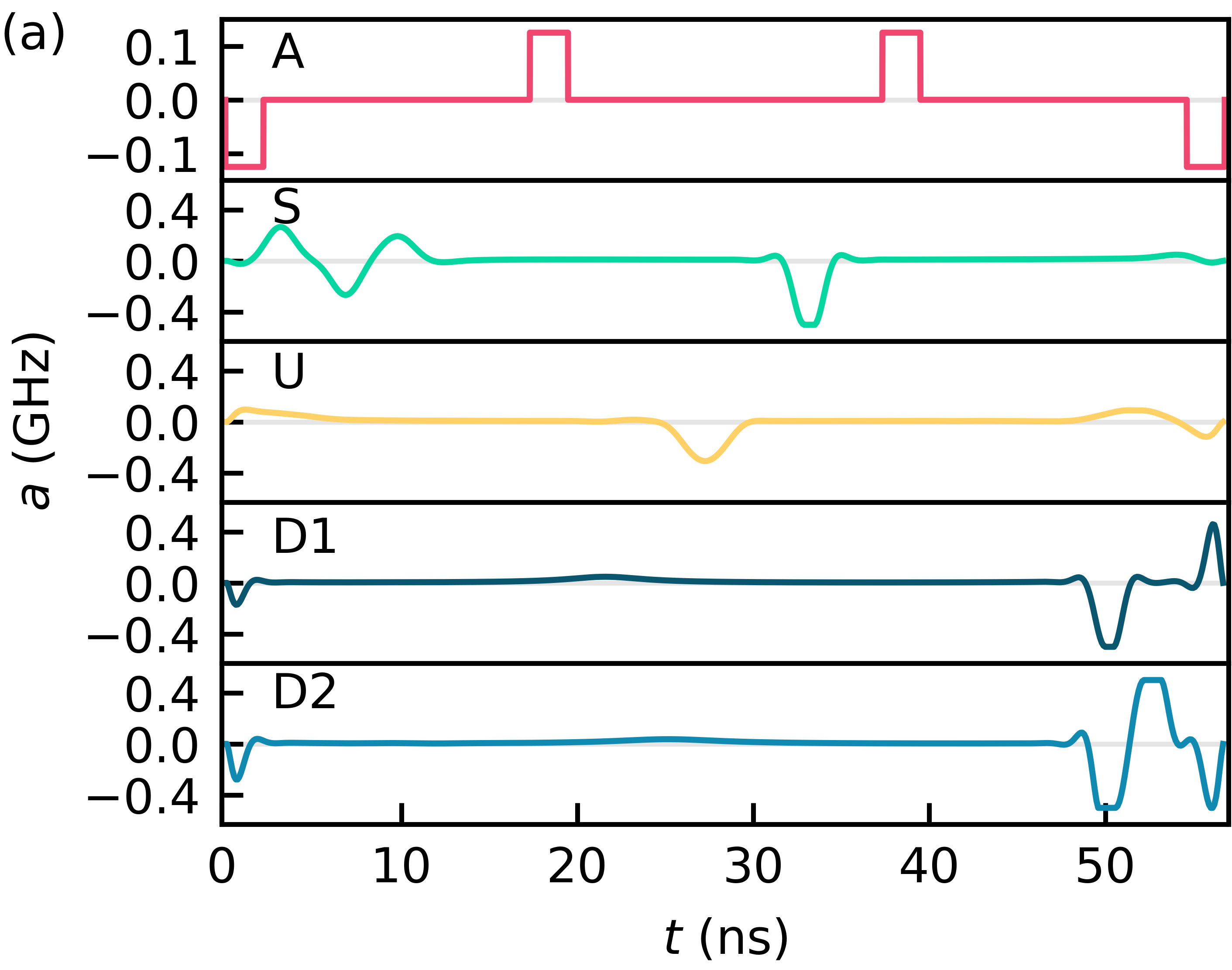
(a)

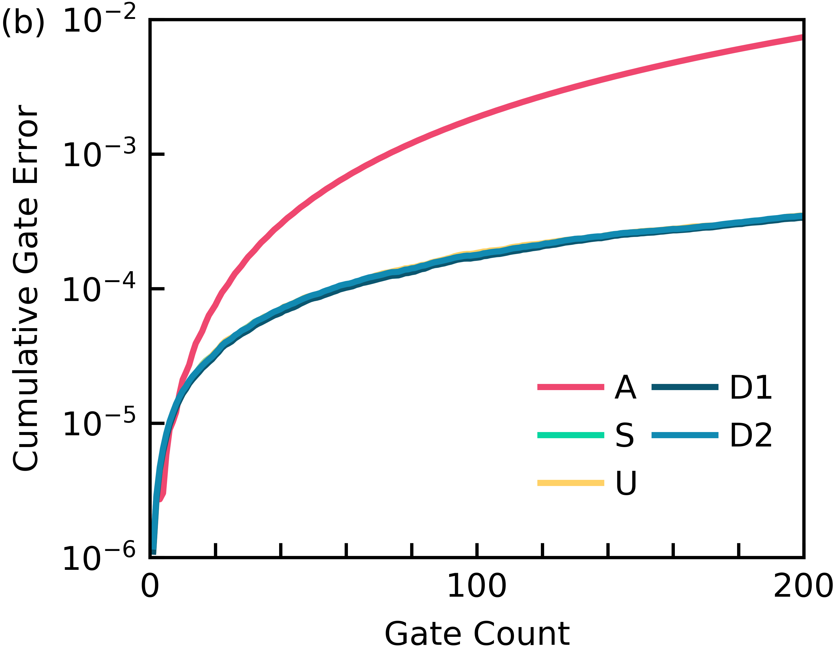
(b)

FIG. 3: (a) Flux pulses for $X/2$ gates robust to flux noise constructed with the analytic (A), sampling (S), unscented sampling (U), and the 1^st- and 2^nd-order derivative methods (D1, D2). (b) Cumulative gate error due to 1/$f$ flux noise for successive gate applications. The cumulative gate errors for the sampling, unscented sampling, and the derivative methods are indistinguishable.

VI Robustness to Time-Dependent Parameter Uncertainty

An additional source of experimental error arises from time-dependent parameter uncertainty. For many flux-biased and inductively-coupled superconducting circuit elements, magnetic flux noise is the dominant source of coherent errors [117, 118, 119, 120]. Flux noise modifies the fluxonium Hamiltonian (2) by $a(t)\rightarrow a(t)+\delta a(t)$ where $\delta a(t)$ is the flux noise. The spectral density of flux noise is observed to follow a 1/$f$ distribution [117, 121, 118, 119, 120, 122, 73], so the noise is dominated by low-frequency components. The analytic gate considered here takes advantage of the low-frequency characteristic and treats the noise as quasi-static, performing a generalization of the spin-echo technique to compensate for erroneous drift [123, 124].

We modify the robust control techniques presented in the previous section to combat 1/$f$ flux noise. The unscented sampling method is modified so that the sample states are subject to 1/$f$ flux noise. The noise is generated by filtering white noise sampled from a standard normal distribution with a finite impulse response filter [125]. The noise is then scaled by the flux noise amplitude of our device $A_{\Phi}=5.21\mu\Phi_{0}\implies\sigma_{a}=2.5\cdot 10^{-5}\textrm{GHz}$. In principle, we could modify the sampling method similarly; however, we choose to subject the sample states to static noise $a(t)\rightarrow a(t)\pm\sigma_{a}$ for comparison. The derivative methods require no algorithmic modification from the static case, but the TDSE is now differentiated with respect to $a(t)$ instead of $f_{q}$ as in (7).

We analyze the gate errors due to 1/$f$ flux noise for the $X/2$ gates constructed with the robust control techniques and the analytic $X/2$ gate. To compute the gate error, we evolve an initial state under the fluxonium Hamiltonian (2) where the optimized flux is modified $a(t)\rightarrow a(t)+\delta a(t)$. We generate the flux noise as we described for the unscented sampling method. The reported gate error is the infidelity averaged over $1000$ pseudorandomly generated initial states, each of which is subject to a distinct pseudorandomly generated flux noise instance. To observe the effect of interfering coherent errors, we simulate successive applications of the gate constructed by each method; we compute the cumulative gate error after each application, see Fig. 3. Both the analytic and numerical gates yield single-gate errors sufficient for quantum error correction. Despite converging on qualitatively different solutions, the numerical gates perform similarly in the concatenated gate application comparison. Their gate errors after $200$ gate applications $\sim 11\mu\textrm{s}$ are two orders of magnitude less than the gate error produced by the analytic gate. 1/$f$ flux noise is a significant source of coherent errors in NISQ applications, and these numerical techniques offer effective avenues to mitigate it.

VII Conclusion

We have introduced state-of-the-art trajectory optimization techniques in the context of quantum optimal control, enabling us to achieve tight tolerances for multiple constraints on the control fields and quantum states. Using these capabilities, we have mitigated decoherence and achieved robustness to parameter uncertainty errors on a superconducting fluxonium qubit. We have proposed a scheme for suppressing depolarization with time-optimal control and the integrated depolarization rate model. The computational complexity of evaluating this model is independent of the dimension of the Hilbert space, enabling inexpensive optimization on high-dimensional quantum systems. We have also proposed the derivative method for robust control which achieves superlinear gate error reductions in the gate time for the static parameter uncertainty problem we studied. We have shown that the derivative, sampling, and unscented sampling methods can mitigate 1/$f$ flux noise errors – which dominate coherent errors for flux controlled qubits. These robust control techniques can be applied to any Hamiltonian, allowing experimentalists in all domains to engineer robust operations on their quantum systems. Furthermore, they can be used to achieve the low gate errors required for fault-tolerant quantum computing applications. Our implementations of the techniques described in this work are available at https://github.com/SchusterLab/rbqoc.

Appendix A Depolarization

We comment on the depolarization metrics and then give our procedure for integrating the Lindblad master equation. The integrated depolarization rate and the gate error due to depolarization are compared in Table 1 for the numerical experiment described in Sec. IV. The ratio of the value obtained on the metric with the analytic technique to the value obtained with the numerical technique is similar across the two metrics.

Gate	$D_{1\textrm{A}}$	$D_{1\textrm{N}}$	$\dfrac{D_{1\textrm{A}}}{D_{1\textrm{N}}}$	$\textrm{GE}_{\textrm{A}}$	$\textrm{GE}_{\textrm{N}}$	$\dfrac{\textrm{GE}_{\textrm{A}}}{\textrm{GE}_{\textrm{N}}}$
	$(10^{-5})$	$(10^{-5})$		$(10^{-5})$	$(10^{-5})$
Z/2	5.745	1.149	5.000	0.888	0.185	4.791
Y/2	5.253	1.157	4.540	0.770	0.186	4.132
X/2	16.251	2.660	6.109	2.674	0.432	6.200

TABLE 1: Single-gate integrated depolarization rate ($D_{1}$) and single-gate error due to depolarization (GE). Values are reported for the analytic (A) and numerical (N) gates.

We employ the Lindblad master equation to compute the gate error due to depolarization. This equation takes the form:

$$\frac{d}{dt}\rho=-\frac{i}{\hbar}[H,\rho]+\sum_{i}\gamma_{i}(L_{i}\rho L_{i}^{\dagger}-\frac{1}{2}\{L_{i}^{\dagger}L_{i},\rho\}),$$ (8)

For depolarization, $\gamma_{\pm}=T_{\pm}^{-1}$, $L_{\pm}=\sigma^{\pm}\equiv(\sigma_{x}\pm i\sigma_{y})/2$. Our device operates in the regime where $hf\ll k_{\textrm{B}}T$ such that $T_{+}=T_{-}=2T_{1}$, where $T_{1}$ is obtained at each time step from the spline shown in Fig. 1(b). We obtain the $T_{1}$ values in this spline by driving the qubit at the desired flux bias and monitoring the resultant decay. For more details on these measurements, consult Ref. [73]. Because $T_{1}$ depends on the flux, so do the decay rates $\gamma_{\pm}$. Integrating the master equation with time-dependent decay rates provides a heuristic for how gates might perform in the experiment. This procedure may not be strictly correct when decay rates change significantly on the time scale of the relaxation time, which is the regime we are operating in. Standard derivations of the Lindblad master equation do not account for time-dependent decay rates [132]. A more thorough treatment of this regime in future work would unlock new insights for quantum computing platforms where decoherence is strongly dependent on the control parameters.

In order to use exponential integrators, we employ the vector (Choi-Jamiolkowski) isomorphism [133],

$$\frac{d}{dt}\textrm{vec}({\rho})=\hat{\mathcal{L}}\,\textrm{vec}({\rho}),$$ (9)

$$\hat{\mathcal{L}} =-i(\openone\otimes H-H^{T}\otimes\openone)$$ (10)

$$+\sum_{i}\gamma_{i}(L_{i}^{*}\otimes L_{i}-\frac{1}{2}(\openone\otimes L_{i}^{\dagger}L_{i}-L_{i}^{T}L_{i}^{*}\otimes\openone)),$$

where $\rho=\sum_{i,j}\alpha_{ij}\ket{i}\bra{j}$ and $\textrm{vec}(\rho)=\sum_{i,j}\alpha_{ij}\ket{i}\otimes\ket{j}$. Because the flux is constant between time steps due to our numerical discretization, the Hamiltonian and decay rates are also constant between time steps. Therefore, the exact solution to (9) is,

$$\textrm{vec}(\rho_{k+1})={\exp}{\textstyle(}\Delta t_{k}\hat{\mathcal{L}}_{k}{\textstyle)}\textrm{vec}(\rho_{k}).$$ (11)

The vector isomorphism transforms $(n\times n)\times(n\times n)$ matrix-matrix multiplications to $(n^{2}\times n^{2})\times n^{2}$ matrix-vector multiplications. For small $n$, we find that it is faster to use an exponential integrator on the vectorized equation than to perform Runge-Kutta on the unvectorized equation. The latter requires decreasing the interval $\Delta t_{k}$ to maintain accuracy, resulting in more time steps.

Appendix B Unscented Sampling Method

In this section, we outline the full unscented sampling procedure. We consider a state $\psi\in\mathbb{R}^{2n}$, an uncertain set of parameters $\lambda\in\mathbb{R}^{d}$, and discrete dynamics $\psi_{k+1}=f(\psi_{k},\lambda_{k})$. The nominal initial state is given by $\bar{\psi}_{1}$ with an associated covariance matrix $P_{1}\in\mathbb{S}_{++}^{2n}$ which describes the uncertainty in the initial state. We use the notation $\mathbb{S}_{++}^{m}$ to denote the set of real, symmetric, and positive-definite $m\times m$ matrices. By the positive-definite requirement, $P_{1}$ must be non-zero even if the state-preparation error is negligible. The uncertain parameter has zero-mean and its distribution is given by the covariance matrix $L_{k}\in\mathbb{S}_{++}^{d}$ at time step $k$. The zero-mean assumption is convenient for deriving the update procedure. A non-zero mean can be encoded in the discrete dynamics function $f(\psi_{k},\lambda_{k})$.

The initial $4n+2d$ sample states and initial $4n+2d$ uncertain parameters are sampled from the initial distributions,

$$\begin{pmatrix}\psi_{1}^{j}\\ \lambda_{1}^{j}\end{pmatrix}=\begin{pmatrix}\bar{\psi}_{1}\\ 0\end{pmatrix}\pm\beta\sqrt{\begin{pmatrix}P_{1}&0\\ 0&L_{1}\end{pmatrix}}^{\;j}.$$ (12)

Here, $\beta$ is a hyperparameter that controls the spacing of the covariance contour. The $(\pm)$ is understood to take $(+)$ for $j\in\{1,\dots,2n+d\}$ and $(-)$ for $j\in\{2n+d+1,\dots,4n+2d\}$. We use the Cholesky factorization to compute the square root of the joint covariance matrix, though other methods such as the principal square root may be employed. The superscript on the matrix square root indicates the $j$^th column (mod $2n+d$) of the lower triangular Cholesky factor. Then, the sample states are normalized,

$$\psi_{1}^{j}\rightarrow\frac{\psi_{1}^{j}}{\sqrt{{\psi_{1}^{j}}^{T}\psi_{1}^{j}}}.$$ (13)

The sample states are propagated to the next time step,

$$\psi^{j}_{2}=f(\psi^{j}_{1},\lambda^{j}_{1}).$$ (14)

The mean and covariance of the sample states are computed,

$$\bar{\psi}_{2} =\frac{1}{4n+2d}\sum_{j=1}^{4n+2d}\psi_{2}^{j},$$ (15)

$$P_{2} =\frac{1}{2\beta^{2}}\sum_{j=1}^{4n+2d}(\psi^{j}_{2}-\bar{\psi}_{2})(\psi^{j}_{2}-\bar{\psi}_{2})^{T}.$$ (16)

The sample states are then resampled and propagated to the next time step using (12), (13), and (14). Our choice of sample states (sigma points) follows equation 11 of Ref. [71]. Prescriptions that require fewer sigma points exist [134].

Appendix C Derivative Method

Here, we outline how to efficiently integrate the dynamics for the derivative method using exponential integrators. General exponential integrators break the dynamics into a linear term and a non-linear term. For example, the dynamics for the first state derivative are,

$$\frac{d}{dt}\ket{\partial_{\lambda}\psi}=-\frac{i}{\hbar}H\ket{\partial_{\lambda}\psi}-\frac{i}{\hbar}(\partial_{\lambda}H)\ket{\psi}.$$ (17)

The linear term is $L=-\frac{i}{\hbar}H$ and the non-linear term is $N=-\frac{i}{\hbar}(\partial_{\lambda}H)\ket{\psi}$. With piecewise-constant controls, the exact solution to (17) is,

$$\ket{\partial_{\lambda}\psi_{k+1}} =\exp(\Delta t_{k}L_{k})\ket{\partial_{\lambda}\psi_{k}}$$ (18)

$$+\int_{0}^{\Delta t_{k}}\exp((\Delta t_{k}-t^{{}^{\prime}})L_{k})N(t_{k}+t^{{}^{\prime}})dt^{{}^{\prime}}.$$

General exponential integrators proceed by breaking the integral in (18) into a discrete sum, similar to the procedure for Runge-Kutta schemes. We use a simple approximation known as the Lawson-Euler method [82],

$$\ket{\partial_{\lambda}\psi_{k+1}} \approx\exp(\Delta t_{k}L_{k})\ket{\partial_{\lambda}\psi_{k}}$$ (19)

$$+\exp(\Delta t_{k}L_{k})N_{k}\Delta t_{k}.$$

This method provides a good tradeoff between accuracy and efficiency, requiring one unique matrix exponential computation per stage. Integration accuracy for the state derivatives is not of the utmost importance because they are used in the robustness cost function – as opposed to the states themselves which are experimental parameters that must be realized with high accuracy.

Appendix D Computational Performance

In this section we provide runtimes for our optimizations. The runtimes for the base optimization in Sec. III, the depolarization optimization in Sec. IV, and the robust optimizations in Sec. V are presented in Table 2 for a $Z/2$ gate at gate times which are multiples of $1/4f_{q}\sim 18$ns. We performed optimizations on a single core of an AMD Ryzen Threadripper 3970X 32-Core Processor @ 3.7 GHz. Future work will parallelize the robustness methods using GPUs [17], which will enable fast optimizations on high-dimensional Hilbert spaces.

	$18$	$36$	$72$
Base	$0.155\pm 0.008$	$7.0\pm 0.4$	$15.9\pm 0.8$
Depol.	$1.69\pm 0.08$	-	-
S	$1.77\pm 0.09$	$48\pm 2$	$280\pm 10$
U	$75\pm 4$	$340\pm 20$	$400\pm 20$
D1	$6.1\pm 0.3$	$27\pm 1$	$65\pm 3$
D2	$15.7\pm 0.8$	$17.3\pm 0.9$	$54\pm 3$

TABLE 2: Average runtimes in seconds for $Z/2$ optimizations using the base, depolarization, sampling (S), unscented sampling (U), and the 1^st- and 2^nd-order derivative methods (D1, D2).

References

- Vandersypen and Chuang [2005] L. M. K. Vandersypen and I. L. Chuang, NMR techniques for quantum control and computation, Rev. Mod. Phys. 76, 1037 (2005).
- Kehlet et al. [2004] C. T. Kehlet, A. C. Sivertsen, M. Bjerring, T. O. Reiss, N. Khaneja, S. J. Glaser, and N. C. Nielsen, Improving Solid-State NMR Dipolar Recoupling by Optimal Control, J. Am. Chem. Soc. 126, 10202 (2004).
- Khaneja et al. [2005] N. Khaneja, T. Reiss, C. Kehlet, T. Schulte-Herbrüggen, and S. J. Glaser, Optimal control of coupled spin dynamics: design of NMR pulse sequences by gradient ascent algorithms, J. Magn. Reson. 172, 296 (2005).
- Maximov et al. [2008] I. I. Maximov, Z. Tošner, and N. C. Nielsen, Optimal control design of NMR and dynamic nuclear polarization experiments using monotonically convergent algorithms, J. Chem. Phys. 128, 184505 (2008).
- Nielsen et al. [2010] N. C. Nielsen, C. Kehlet, S. J. Glaser, and N. Khaneja, Optimal Control Methods in NMR Spectroscopy, in eMagRes (American Cancer Society, 2010).
- Skinner et al. [2003] T. E. Skinner, T. O. Reiss, B. Luy, N. Khaneja, and S. J. Glaser, Application of optimal control theory to the design of broadband excitation pulses for high-resolution NMR, J. Magn. Reson. 163, 8 (2003).
- Tošner et al. [2009] Z. Tošner, T. Vosegaard, C. Kehlet, N. Khaneja, S. J. Glaser, and N. C. Nielsen, Optimal control in NMR spectroscopy: Numerical implementation in SIMPSON, J. Magn. Reson. 197, 120 (2009).
- Abdelhafez et al. [2020] M. Abdelhafez, B. Baker, A. Gyenis, P. Mundada, A. A. Houck, D. Schuster, and J. Koch, Universal gates for protected superconducting qubits using optimal control, Phys. Rev. A 101, 022321 (2020).
- Chakram et al. [2020] S. Chakram, K. He, A. V. Dixit, A. E. Oriani, R. K. Naik, N. Leung, H. Kwon, W.-L. Ma, L. Jiang, and D. I. Schuster, Multimode photon blockade (2020), arXiv:2010.15292 [quant-ph] .
- Egger and Wilhelm [2013] D. J. Egger and F. K. Wilhelm, Optimized controlled-Z gates for two superconducting qubits coupled through a resonator, Supercond. Sci. Technol. 27, 014001 (2013).
- Fisher et al. [2010] R. Fisher, F. Helmer, S. J. Glaser, F. Marquardt, and T. Schulte-Herbrüggen, Optimal control of circuit quantum electrodynamics in one and two dimensions, Phys. Rev. B 81, 085328 (2010).
- Gokhale et al. [2019] P. Gokhale, Y. Ding, T. Propson, C. Winkler, N. Leung, Y. Shi, D. I. Schuster, H. Hoffmann, and F. T. Chong, Partial Compilation of Variational Algorithms for Noisy Intermediate-Scale Quantum Machines, in Proceedings of the 52nd Annual IEEE/ACM International Symposium on Microarchitecture (2019) pp. 266–278.
- Huang and Goan [2014] S.-Y. Huang and H.-S. Goan, Optimal control for fast and high-fidelity quantum gates in coupled superconducting flux qubits, Phys. Rev. A 90, 012318 (2014).
- Heeres et al. [2017] R. W. Heeres, P. Reinhold, N. Ofek, L. Frunzio, L. Jiang, M. H. Devoret, and R. J. Schoelkopf, Implementing a universal gate set on a logical qubit encoded in an oscillator, Nat. Commun. 8, 1 (2017).
- Kelly et al. [2014] J. Kelly, R. Barends, B. Campbell, Y. Chen, Z. Chen, B. Chiaro, A. Dunsworth, A. G. Fowler, I.-C. Hoi, E. Jeffrey, A. Megrant, J. Mutus, C. Neill, P. J. J. O’Malley, C. Quintana, P. Roushan, D. Sank, A. Vainsencher, J. Wenner, T. C. White, A. N. Cleland, and J. M. Martinis, Optimal Quantum Control Using Randomized Benchmarking, Phys. Rev. Lett. 112, 240504 (2014).
- Leng et al. [2019] Z. Leng, P. Mundada, S. Ghadimi, and A. Houck, Robust and efficient algorithms for high-dimensional black-box quantum optimization (2019), arXiv:1910.03591 [quant-ph] .
- Leung et al. [2017] N. Leung, M. Abdelhafez, J. Koch, and D. Schuster, Speedup for quantum optimal control from automatic differentiation based on graphics processing units, Phys. Rev. A 95, 042318 (2017).
- Li et al. [2020] S. Li, T. Chen, and Z.-Y. Xue, Fast Holonomic Quantum Computation on Superconducting Circuits With Optimal Control, Adv. Quantum Technol. 3, 2000001 (2020).
- Liebermann and Wilhelm [2016] P. J. Liebermann and F. K. Wilhelm, Optimal Qubit Control Using Single-Flux Quantum Pulses, Phys. Rev. Applied 6, 024022 (2016).
- Reinhold [2019] P. Reinhold, Controlling Error-Correctable Bosonic Qubits, Ph.D. thesis, Yale University (2019).
- Rebentrost and Wilhelm [2009] P. Rebentrost and F. K. Wilhelm, Optimal control of a leaking qubit, Phys. Rev. B 79, 060507 (2009).
- Rebentrost et al. [2009] P. Rebentrost, I. Serban, T. Schulte-Herbrüggen, and F. K. Wilhelm, Optimal Control of a Qubit Coupled to a Non-Markovian Environment, Phys. Rev. Lett. 102, 090401 (2009).
- Spiteri et al. [2018] R. J. Spiteri, M. Schmidt, J. Ghosh, E. Zahedinejad, and B. C. Sanders, Quantum control for high-fidelity multi-qubit gates, New J. Phys. 20, 113009 (2018).
- Spörl et al. [2007] A. Spörl, T. Schulte-Herbrüggen, S. J. Glaser, V. Bergholm, M. J. Storcz, J. Ferber, and F. K. Wilhelm, Optimal control of coupled Josephson qubits, Phys. Rev. A 75, 012302 (2007).
- Brouzos et al. [2015] I. Brouzos, A. I. Streltsov, A. Negretti, R. S. Said, T. Caneva, S. Montangero, and T. Calarco, Quantum speed limit and optimal control of many-boson dynamics, Phys. Rev. A 92, 062110 (2015).
- De Chiara et al. [2008] G. De Chiara, T. Calarco, M. Anderlini, S. Montangero, P. J. Lee, B. L. Brown, W. D. Phillips, and J. V. Porto, Optimal control of atom transport for quantum gates in optical lattices, Phys. Rev. A 77, 052333 (2008).
- Grace et al. [2007] M. Grace, C. Brif, H. Rabitz, I. A. Walmsley, R. L. Kosut, and D. A. Lidar, Optimal control of quantum gates and suppression of decoherence in a system of interacting two-level particles, J. Phys. B: At. Mol. Opt. Phys. 40, S103 (2007).
- Goerz et al. [2011] M. H. Goerz, T. Calarco, and C. P. Koch, The quantum speed limit of optimal controlled phasegates for trapped neutral atoms, J. Phys. B: At. Mol. Opt. Phys. 44, 154011 (2011).
- Guo et al. [2019] J. Guo, X. Feng, P. Yang, Z. Yu, L. Q. Chen, C.-H. Yuan, and W. Zhang, High-performance Raman quantum memory with optimal control in room temperature atoms, Nat. Commun. 10, 148 (2019).
- Jensen et al. [2019] J. H. M. Jensen, J. J. Sørensen, K. Mølmer, and J. F. Sherson, Time-optimal control of collisional gates in ultracold atomic systems, Phys. Rev. A 100, 052314 (2019).
- Larrouy et al. [2020] A. Larrouy, S. Patsch, R. Richaud, J.-M. Raimond, M. Brune, C. P. Koch, and S. Gleyzes, Fast Navigation in a Large Hilbert Space Using Quantum Optimal Control, Phys. Rev. X 10, 021058 (2020).
- Nebendahl et al. [2009] V. Nebendahl, H. Häffner, and C. F. Roos, Optimal control of entangling operations for trapped-ion quantum computing, Phys. Rev. A 79, 012312 (2009).
- Omran et al. [2019] A. Omran, H. Levine, A. Keesling, G. Semeghini, T. T. Wang, S. Ebadi, H. Bernien, A. S. Zibrov, H. Pichler, S. Choi, J. Cui, M. Rossignolo, P. Rembold, S. Montangero, T. Calarco, M. Endres, M. Greiner, V. Vuletić, and M. D. Lukin, Generation and manipulation of schrödinger cat states in rydberg atom arrays, Science 365, 570 (2019).
- Rosi et al. [2013] S. Rosi, A. Bernard, N. Fabbri, L. Fallani, C. Fort, M. Inguscio, T. Calarco, and S. Montangero, Fast closed-loop optimal control of ultracold atoms in an optical lattice, Phys. Rev. A 88, 021601 (2013).
- Treutlein et al. [2006] P. Treutlein, T. W. Hänsch, J. Reichel, A. Negretti, M. A. Cirone, and T. Calarco, Microwave potentials and optimal control for robust quantum gates on an atom chip, Phys. Rev. A 74, 022312 (2006).
- van Frank et al. [2016] S. van Frank, M. Bonneau, J. Schmiedmayer, S. Hild, C. Gross, M. Cheneau, I. Bloch, T. Pichler, A. Negretti, T. Calarco, et al., Optimal control of complex atomic quantum systems, Sci. Rep. 6, 34187 (2016).
- Chou et al. [2015] Y. Chou, S.-Y. Huang, and H.-S. Goan, Optimal control of fast and high-fidelity quantum gates with electron and nuclear spins of a nitrogen-vacancy center in diamond, Phys. Rev. A 91, 052315 (2015).
- Dolde et al. [2014] F. Dolde, V. Bergholm, Y. Wang, I. Jakobi, B. Naydenov, S. Pezzagna, J. Meijer, F. Jelezko, P. Neumann, T. Schulte-Herbrüggen, et al., High-fidelity spin entanglement using optimal control, Nat. Commun. 5, 1 (2014).
- Geng et al. [2016] J. Geng, Y. Wu, X. Wang, K. Xu, F. Shi, Y. Xie, X. Rong, and J. Du, Experimental Time-Optimal Universal Control of Spin Qubits in Solids, Phys. Rev. Lett. 117, 170501 (2016).
- Nöbauer et al. [2015] T. Nöbauer, A. Angerer, B. Bartels, M. Trupke, S. Rotter, J. Schmiedmayer, F. Mintert, and J. Majer, Smooth Optimal Quantum Control for Robust Solid-State Spin Magnetometry, Phys. Rev. Lett. 115, 190801 (2015).
- Poggiali et al. [2018] F. Poggiali, P. Cappellaro, and N. Fabbri, Optimal Control for One-Qubit Quantum Sensing, Phys. Rev. X 8, 021059 (2018).
- Rembold et al. [2020] P. Rembold, N. Oshnik, M. M. Müller, S. Montangero, T. Calarco, and E. Neu, Introduction to quantum optimal control for quantum sensing with nitrogen-vacancy centers in diamond, AVS Quantum Sci. 2, 024701 (2020).
- Tian et al. [2019] J. Tian, T. Du, Y. Liu, H. Liu, F. Jin, R. S. Said, and J. Cai, Optimal quantum optical control of spin in diamond, Phys. Rev. A 100, 012110 (2019).
- Amri et al. [2019] S. Amri, R. Corgier, D. Sugny, E. M. Rasel, N. Gaaloul, and E. Charron, Optimal control of the transport of Bose-Einstein condensates with atom chips, Sci. Rep. 9, 1 (2019).
- Doria et al. [2011] P. Doria, T. Calarco, and S. Montangero, Optimal Control Technique for Many-Body Quantum Dynamics, Phys. Rev. Lett. 106, 190501 (2011).
- Sørensen et al. [2019] J. J. Sørensen, J. Jensen, T. Heinzel, and J. F. Sherson, QEngine: A C++ library for quantum optimal control of ultracold atoms, Comput. Phys. Commun. 243, 135 (2019).
- Sørensen et al. [2018] J. J. W. H. Sørensen, M. O. Aranburu, T. Heinzel, and J. F. Sherson, Quantum optimal control in a chopped basis: Applications in control of Bose-Einstein condensates, Phys. Rev. A 98, 022119 (2018).
- Klimov et al. [2020] P. V. Klimov, J. Kelly, J. M. Martinis, and H. Neven, The Snake Optimizer for Learning Quantum Processor Control Parameters (2020), arXiv:2006.04594 [quant-ph] .
- Zhou [1997] K. Zhou, Essentials of Robust Control, 1st ed. (Pearson, 1997).
- Morimoto and Atkeson [2002] J. Morimoto and C. Atkeson, Minimax Differential Dynamic Programming: An Application to Robust Biped Walking, Adv. neural inf. process. syst. 15, 1563 (2002).
- Manchester and Kuindersma [2018] Z. Manchester and S. Kuindersma, Robust direct trajectory optimization using approximate invariant funnels, Auton. Robot. 10.1007/s10514-018-9779-5 (2018).
- Cummins and Jones [2000] H. K. Cummins and J. A. Jones, Use of composite rotations to correct systematic errors in NMR quantum computation, New J. Phys. 2, 6 (2000).
- Cummins et al. [2003] H. K. Cummins, G. Llewellyn, and J. A. Jones, Tackling systematic errors in quantum logic gates with composite rotations, Phys. Rev. A 67, 042308 (2003).
- Kupce and Freeman [1995] Ä. Kupce and R. Freeman, Stretched Adiabatic Pulses for Broadband Spin Inversion, J. Magn. Reson., Series A 117, 246 (1995).
- Merrill and Brown [2014] J. T. Merrill and K. R. Brown, Progress in compensating pulse sequences for quantum computation, Quantum Information and Computation for Chemistry , 241 (2014).
- Han et al. [2020] Z. Han, Y. Dong, B. Liu, X. Yang, S. Song, L. Qiu, D. Li, J. Chu, W. Zheng, J. Xu, et al., Experimental Realization of Universal Time-optimal non-Abelian Geometric Gates (2020), arXiv:2004.10364 [quant-ph] .
- Xu et al. [2020] J. Xu, S. Li, T. Chen, and Z.-Y. Xue, Nonadiabatic geometric quantum computation with optimal control on superconducting circuits (2020), arXiv:2004.10199 [quant-ph] .
- Motzoi et al. [2009] F. Motzoi, J. M. Gambetta, P. Rebentrost, and F. K. Wilhelm, Simple Pulses for Elimination of Leakage in Weakly Nonlinear Qubits, Phys. Rev. Lett. 103, 110501 (2009).
- Egger and Wilhelm [2014] D. J. Egger and F. K. Wilhelm, Adaptive Hybrid Optimal Quantum Control for Imprecisely Characterized Systems, Phys. Rev. Lett. 112, 240503 (2014).
- Feng et al. [2018] G. Feng, F. H. Cho, H. Katiyar, J. Li, D. Lu, J. Baugh, and R. Laflamme, Gradient-based closed-loop quantum optimal control in a solid-state two-qubit system, Phys. Rev. A 98, 052341 (2018).
- Li et al. [2017] J. Li, X. Yang, X. Peng, and C.-P. Sun, Hybrid Quantum-Classical Approach to Quantum Optimal Control, Phys. Rev. Lett. 118, 150503 (2017).
- Wittler et al. [2020] N. Wittler, F. Roy, K. Pack, M. Werninghaus, A. S. Roy, D. J. Egger, S. Filipp, F. K. Wilhelm, and S. Machnes, An integrated tool-set for Control, Calibration and Characterization of quantum devices applied to superconducting qubits (2020), arXiv:2009.09866 [quant-ph] .
- Ball et al. [2021] H. Ball, M. Biercuk, A. Carvalho, J. Chen, M. R. Hush, L. A. de Castro, L. Li, P. J. Liebermann, H. Slatyer, C. Edmunds, V. Frey, C. Hempel, and A. Milne, Software tools for quantum control: Improving quantum computer performance through noise and error suppression, Quantum Sci. Technol. 10.1088/2058-9565/abdca6 (2021).
- Carvalho et al. [2020] A. R. Carvalho, H. Ball, M. J. Biercuk, M. R. Hush, and F. Thomsen, Error-robust quantum logic optimization using a cloud quantum computer interface (2020), arXiv:2010.08057 [quant-ph] .
- Allen [2019] J. Allen, Robust Optimal Control of the Cross-Resonance Gate in Superconducting Qubits, Ph.D. thesis, University of Surrey (2019).
- Kosut et al. [2013] R. L. Kosut, M. D. Grace, and C. Brif, Robust control of quantum gates via sequential convex programming, Phys. Rev. A 88, 052326 (2013).
- Niu et al. [2019] M. Y. Niu, S. Boixo, V. N. Smelyanskiy, and H. Neven, Universal quantum control through deep reinforcement learning, NPJ Quantum Inf. 5, 33 (2019).
- Howell et al. [2020] T. A. Howell, C. Fu, and Z. Manchester, Direct Policy Optimization using Deterministic Sampling and Collocation (2020), arXiv:2010.08506 [cs.RO] .
- Lee et al. [2013] A. Lee, Y. Duan, S. Patil, J. Schulman, Z. McCarthy, J. van den Berg, K. Goldberg, and P. Abbeel, Sigma hulls for Gaussian belief space planning for imprecise articulated robots amid obstacles, in 2013 IEEE/RSJ International Conference on Intelligent Robots and Systems (2013) pp. 5660–5667.
- Thangavel et al. [2020] S. Thangavel, R. Paulen, and S. Engell, Robust Multi-Stage Nonlinear Model Predictive Control Using Sigma Points, Processes 8, 851 (2020).
- Julier and Uhlmann [2004] S. J. Julier and J. K. Uhlmann, Unscented filtering and nonlinear estimation, Proceedings of the IEEE 92, 401 (2004).
- Uhlmann [1995] J. K. Uhlmann, Dynamic Map Building and Localization: New Theoretical Foundations, Ph.D. thesis, University of Oxford Oxford (1995).
- Zhang et al. [2021] H. Zhang, S. Chakram, T. Roy, N. Earnest, Y. Lu, Z. Huang, D. K. Weiss, J. Koch, and D. I. Schuster, Universal Fast-Flux Control of a Coherent, Low-Frequency Qubit, Phys. Rev. X 11, 011010 (2021).
- Howell et al. [2019] T. A. Howell, B. E. Jackson, and Z. Manchester, ALTRO: A fast solver for constrained trajectory optimization, in 2019 IEEE/RSJ International Conference on Intelligent Robots and Systems (IROS) (IEEE, 2019) pp. 7674–7679.
- Machnes et al. [2018] S. Machnes, E. Assémat, D. Tannor, and F. K. Wilhelm, Tunable, Flexible, and Efficient Optimization of Control Pulses for Practical Qubits, Phys. Rev. Lett. 120, 150401 (2018).
- Goerz et al. [2019] M. H. Goerz, D. Basilewitsch, F. Gago-Encinas, M. G. Krauss, K. P. Horn, D. M. Reich, and C. P. Koch, Krotov: A Python implementation of Krotov’s method for quantum optimal control, SciPost Phys. 7, 10.21468/SciPostPhys.7.6.080 (2019).
- Schulman et al. [2013] J. Schulman, J. Ho, A. X. Lee, I. Awwal, H. Bradlow, and P. Abbeel, Finding Locally Optimal, Collision-Free Trajectories with Sequential Convex Optimization., in Robotics: science and systems, Vol. 9 (Citeseer, 2013) pp. 1–10.
- Tedrake and the Drake Development Team [2016] R. Tedrake and the Drake Development Team, Drake: A planning, control, and analysis toolbox for nonlinear dynamical systems (2016).
- Hereid and Ames [2017] A. Hereid and A. D. Ames, FROST: Fast Robot Optimization and Simulation Toolkit, in 2017 IEEE/RSJ International Conference on Intelligent Robots and Systems (IROS) (IEEE, Vancouver, BC, Canada, 2017).
- Jørgensen et al. [2011] L. Jørgensen, D. L. Cardozo, and E. Thibierge, Numerical Resolution Of The Schrödinger Equation, Tech. Rep. (École Normale Supérieure de Lyon, 2011).
- Auer et al. [2018] N. Auer, L. Einkemmer, P. Kandolf, and A. Ostermann, Magnus integrators on multicore CPUs and GPUs, Comput. Phys. Commun. 228, 115 (2018).
- Berland and Skaflestad [2006] H. Berland and B. Skaflestad, Solving the nonlinear Schrödinger equation using exponential integrators, Int. J. Model. Identif. Control. 27, 201 (2006).
- Einkemmer et al. [2017] L. Einkemmer, M. Tokman, and J. Loffeld, On the performance of exponential integrators for problems in magnetohydrodynamics, J. Comput. Phys. 330, 550 (2017).
- Shillito et al. [2020] R. Shillito, J. A. Gross, A. D. Paolo, Élie Genois, and A. Blais, Fast and differentiable simulation of driven quantum systems (2020), arXiv:2012.09282 [quant-ph] .
- Hargraves and Paris [1987] C. R. Hargraves and S. W. Paris, Direct Trajectory Optimization Using Nonlinear Programming and Collocation, J. Guidance 10, 338 (1987).
- Kelly [2017] M. Kelly, An Introduction to Trajectory Optimization: How to Do Your Own Direct Collocation, SIAM Review 59, 849 (2017).
- Betts [1998] J. T. Betts, Survey of Numerical Methods for Trajectory Optimization, J. Guid. Control Dyn 21, 193 (1998).
- Gill et al. [2005] P. E. Gill, W. Murray, and M. A. Saunders, SNOPT: An SQP Algorithm for Large-Scale Constrained Optimization, SIAM review 47, 99 (2005).
- Wächter and Biegler [2006] A. Wächter and L. T. Biegler, On the implementation of an interior-point filter line-search algorithm for large-scale nonlinear programming, Math. Program. 106, 25 (2006).
- Li and Todorov [2004] W. Li and E. Todorov, Iterative Linear Quadratic Regulator Design for Nonlinear Biological Movement Systems, in Proceedings of the 1st International Conference on Informatics in Control, Automation and Robotics (Setubal, Portugal, 2004).
- Lantoine and Russell [2012] G. Lantoine and R. P. Russell, A Hybrid Differential Dynamic Programming Algorithm for Constrained Optimal Control Problems. Part 1: Theory, J. Optim. Theory. Appl. 154, 382 (2012).
- Plancher et al. [2017] B. Plancher, Z. Manchester, and S. Kuindersma, Constrained unscented dynamic programming, in 2017 IEEE/RSJ International Conference on Intelligent Robots and Systems (IEEE, 2017) pp. 5674–5680.
- Nocedal and Wright [2006] J. Nocedal and S. Wright, Numerical Optimization (Springer Science & Business Media, 2006).
- Bertsekas [1982] D. P. Bertsekas, Projected Newton Methods for Optimization Problems with Simple Constraints, SIAM J. Control Optim. 20, 221 (1982).
- Rao et al. [1998] C. V. Rao, S. J. Wright, and J. B. Rawlings, Application of Interior-Point Methods to Model Predictive Control, J. Optim. Theory. Appl. 99, 723 (1998).
- Mayne [1966] D. Q. Mayne, A Second-Order Gradient Method of Optimizing Non-Linear Discrete Time Systems, Int. J. Control 3, 8595 (1966).
- Zhang et al. [2006] L. Zhang, W. Zhou, and D. Li, Global convergence of a modified Fletcher–Reeves conjugate gradient method with Armijo-type line search, Numer. Math. 104, 561 (2006).
- Bertsekas [2014] D. P. Bertsekas, Constrained Optimization and Lagrange Multiplier Methods (Academic press, 2014).
- Jackson et al. [2021] B. E. Jackson, T. Punnoose, D. Neamati, K. Tracy, R. Jitosho, and Z. Manchester, ALTRO-C: A Fast Solver for Conic Model-Predictive Control, in International Conference on Robotics and Automation ICRA (2021) in Review.
- Earnest et al. [2018] N. Earnest, S. Chakram, Y. Lu, N. Irons, R. K. Naik, N. Leung, L. Ocola, D. A. Czaplewski, B. Baker, J. Lawrence, J. Koch, and D. I. Schuster, Realization of a System with Metastable States of a Capacitively Shunted Fluxonium, Phys. Rev. Lett. 120, 150504 (2018).
- Lin et al. [2018] Y.-H. Lin, L. B. Nguyen, N. Grabon, J. San Miguel, N. Pankratova, and V. E. Manucharyan, Demonstration of Protection of a Superconducting Qubit from Energy Decay, Phys. Rev. Lett. 120, 150503 (2018).
- Manucharyan et al. [2009] V. E. Manucharyan, J. Koch, L. I. Glazman, and M. H. Devoret, Fluxonium: Single cooper-pair circuit free of charge offsets, Science 326, 113 (2009).
- Somoroff et al. [2021] A. Somoroff, Q. Ficheux, R. A. Mencia, H. Xiong, R. V. Kuzmin, and V. E. Manucharyan, Millisecond coherence in a superconducting qubit (2021), arXiv:2103.08578 [quant-ph] .
- Nguyen et al. [2019] L. B. Nguyen, Y.-H. Lin, A. Somoroff, R. Mencia, N. Grabon, and V. E. Manucharyan, High-Coherence Fluxonium Qubit, Phys. Rev. X 9, 041041 (2019).
- Rol et al. [2019] M. A. Rol, F. Battistel, F. K. Malinowski, C. C. Bultink, B. M. Tarasinski, R. Vollmer, N. Haider, N. Muthusubramanian, A. Bruno, B. M. Terhal, and L. DiCarlo, Fast, High-Fidelity Conditional-Phase Gate Exploiting Leakage Interference in Weakly Anharmonic Superconducting Qubits, Phys. Rev. Lett. 123, 120502 (2019).
- Krantz et al. [2019] P. Krantz, M. Kjaergaard, F. Yan, T. P. Orlando, S. Gustavsson, and W. D. Oliver, A quantum engineer’s guide to superconducting qubits, Appl. Phys. Rev. 6, 021318 (2019).
- Schulte-Herbrüggen et al. [2011] T. Schulte-Herbrüggen, A. Spörl, N. Khaneja, and S. J. Glaser, Optimal control for generating quantum gates in open dissipative systems, J. Phys. B: At. Mol. Opt. Phys. 44, 154013 (2011).
- Abdelhafez et al. [2019] M. Abdelhafez, D. I. Schuster, and J. Koch, Gradient-based optimal control of open quantum systems using quantum trajectories and automatic differentiation, Phys. Rev. A 99, 052327 (2019).
- Huang et al. [2021] Z. Huang, P. S. Mundada, A. Gyenis, D. I. Schuster, A. A. Houck, and J. Koch, Engineering Dynamical Sweet Spots to Protect Qubits from Noise, Phys. Rev. Applied 15, 034065 (2021).
- Mundada et al. [2020] P. S. Mundada, A. Gyenis, Z. Huang, J. Koch, and A. A. Houck, Floquet-engineered enhancement of coherence times in a driven fluxonium qubit (2020), arXiv:2007.13756 [quant-ph] .
- Aharonov and Ben-Or [2008] D. Aharonov and M. Ben-Or, Fault-Tolerant Quantum Computation with Constant Error Rate, SIAM J. Comput. 38, 1207 (2008).
- Knill [2005] E. Knill, Quantum computing with realistically noisy devices, Nature 434, 39–44 (2005).
- Gottesman [1997] D. Gottesman, Stabilizer Codes and Quantum Error Correction (1997), arXiv:quant-ph/9705052 [quant-ph] .
- Paetznick [2014] A. Paetznick, Resource optimization for fault-tolerant quantum computing, Ph.D. thesis, University of Waterloo (2014).
- Suchara et al. [2013] M. Suchara, A. Faruque, C.-Y. Lai, G. Paz, F. T. Chong, and J. Kubiatowicz, Comparing the Overhead of Topological and concatenated Quantum Error Correction (2013), arXiv:1312.2316 [quant-ph] .
- Chow et al. [2009] J. M. Chow, J. M. Gambetta, L. Tornberg, J. Koch, L. S. Bishop, A. A. Houck, B. R. Johnson, L. Frunzio, S. M. Girvin, and R. J. Schoelkopf, Randomized Benchmarking and Process Tomography for Gate Errors in a Solid-State Qubit, Phys. Rev. Lett. 102, 090502 (2009).
- Bialczak et al. [2007] R. C. Bialczak, R. McDermott, M. Ansmann, M. Hofheinz, N. Katz, E. Lucero, M. Neeley, A. D. O’Connell, H. Wang, A. N. Cleland, and J. M. Martinis, Flux Noise in Josephson Phase Qubits, Phys. Rev. Lett. 99, 187006 (2007).
- Kakuyanagi et al. [2007] K. Kakuyanagi, T. Meno, S. Saito, H. Nakano, K. Semba, H. Takayanagi, F. Deppe, and A. Shnirman, Dephasing of a Superconducting Flux Qubit, Phys. Rev. Lett. 98, 047004 (2007).
- Kumar et al. [2016] P. Kumar, S. Sendelbach, M. A. Beck, J. W. Freeland, Z. Wang, H. Wang, C. C. Yu, R. Q. Wu, D. P. Pappas, and R. McDermott, Origin and Reduction of Magnetic Flux Noise in Superconducting Devices, Phys. Rev. Applied 6, 041001 (2016).
- Yoshihara et al. [2006] F. Yoshihara, K. Harrabi, A. O. Niskanen, Y. Nakamura, and J. S. Tsai, Decoherence of Flux Qubits due to Flux Noise, Phys. Rev. Lett. 97, 167001 (2006).
- Koch et al. [2007] R. H. Koch, D. P. DiVincenzo, and J. Clarke, Model for Flux Noise in SQUIDs and Qubits, Phys. Rev. Lett. 98, 267003 (2007).
- Yoshihara et al. [2010] F. Yoshihara, Y. Nakamura, and J. S. Tsai, Correlated flux noise and decoherence in two inductively coupled flux qubits, Phys. Rev. B 81, 132502 (2010).
- Hahn and Maxwell [1952] E. L. Hahn and D. E. Maxwell, Spin Echo Measurements of Nuclear Spin Coupling in Molecules, Phys. Rev. 88, 1070 (1952).
- Meiboom and Gill [1958] S. Meiboom and D. Gill, Modified Spin‐Echo Method for Measuring Nuclear Relaxation Times, Rev. Sci. Instrum. 29, 688 (1958).
- Smith [2020] J. O. Smith, Spectral Audio Signal Processing (2020) online book, 2011 edition.
- Rackauckas and Nie [2017] C. Rackauckas and Q. Nie, DifferentialEquations.jl – A Performant and Feature-Rich Ecosystem for Solving Differential Equations in Julia, J. Open Res. Softw. 5 (2017).
- Besançon et al. [2019] M. Besançon, D. Anthoff, A. Arslan, S. Byrne, D. Lin, T. Papamarkou, and J. Pearson, Distributions.jl: Definition and Modeling of Probability Distributions in the JuliaStats Ecosystem (2019), arXiv:1907.08611 [stat.CO] .
- Revels et al. [2016] J. Revels, M. Lubin, and T. Papamarkou, Forward-Mode Automatic Differentiation in Julia, arXiv:1607.07892 [cs.MS] (2016).
- Hunter [2007] J. D. Hunter, Matplotlib: A 2D graphics environment, Comput. Sci. Eng. 9, 90 (2007).
- Harris et al. [2020] C. R. Harris, K. J. Millman, S. J. van der Walt, R. Gommers, P. Virtanen, D. Cournapeau, E. Wieser, J. Taylor, S. Berg, N. J. Smith, R. Kern, M. Picus, S. Hoyer, M. H. van Kerkwijk, M. Brett, A. Haldane, J. F. del R’ıo, M. Wiebe, P. Peterson, P. G’erard-Marchant, K. Sheppard, T. Reddy, W. Weckesser, H. Abbasi, C. Gohlke, and T. E. Oliphant, Array programming with NumPy, Nature 585, 357 (2020).
- Innes [2018] M. Innes, Don’t Unroll Adjoint: Differentiating SSA-Form Programs (2018), arXiv:1810.07951 [cs.PL] .
- Manzano [2020] D. Manzano, A short introduction to the lindblad master equation, AIP Adv. 10, 025106 (2020).
- Landi [2018] G. T. Landi, Quantum Information and Quantum Noise (2018).
- Julier and Uhlmann [2002] S. J. Julier and J. K. Uhlmann, Reduced sigma point filters for the propagation of means and covariances through nonlinear transformations, in Proceedings of the 2002 American Control Conference (IEEE Cat. No. CH37301), Vol. 2 (IEEE, 2002) pp. 887–892.