Protective Measurement - a new quantum measurement paradigm: detailed description of the first realisation

Abstract

We present a detailed description of the experiment realising for the first time a protective measurement, a novel measurement protocol which combines weak interactions with a “protection mechanism” preserving the measured state coherence during the whole measurement process. Furthermore, protective measurement allows finding the expectation value of an observable, i.e. an inherently statistical quantity, by measuring a single particle, without the need of any statistics. This peculiar property, in sharp contrast with the framework of traditional (projective) quantum measurement, might constitute a groundbreaking advance for several quantum technology related fields.

I Introduction

Measurement in quantum mechanics is usually described through projective measurements, represented by a projector onto physical states within a given Hilbert space. This kind of measurement induces the wavefunction collapse onto a specific eigenstate of the observable, corresponding to the observed eigenvalue. In contrast with this measurement paradigm, in weak measurements, introduced by Aharonov, Albert and Vaidman [1], the coupling between the pointer and the quantum state is weak, introducing only a partial decoherence of the wavefunction, at the price of acquiring only partial information about the state. Examples of weak-coupling-based schemes are measurement of weak values [1, 2] and protective measurements (PM) [3, 4, 5, 6].

In general, a common property for all quantum measurements is that the measurement procedure is invasive, inducing unavoidable decoherence in the initial state of the system. Even in weak value measurements [1, 2, 20, 22, 40, 8, 9, 10, 11, 12, 13, 21, 14, 15, 16, 17, 18, 19, 23, 24, 25, 26, 27, 28, 29, 30, 31, 32, 33, 7, 34, 35, 36, 37, 38, 39], the coupling between the system and the measuring device causes a small perturbation to the system state. In contrast with other quantum measurement paradigms, a PM is able to preserve the coherence of the quantum state during the whole measurement process, thanks to a protection mechanism or, alternatively, via the adiabatic theorem [3]. This difference with respect to traditional measurement protocols allows PM to extract the expectation value of an observable (so far considered as an inherently statistical quantity, only obtainable by means of repeated measurement of an ensemble of identically-prepared systems) by measuring a single quantum system.

Hence, PM is a novel measurement paradigm presenting significant elements of interest both as a tool for quantum metrology and for understanding the very foundations of quantum measurement and, more generally, of quantum mechanics itself, e.g. the possibility of measuring a stationary wavefunction $\ket{\psi}$ [3]. For this reason, PMs add significant elements to the debate about the ontic or epistemic nature of the wavefunction, a highly debated topic in the scientific community [4, 5, 6, 41, 49, 51, 50, 42, 43, 44, 45, 46, 47, 48, 52, 53, 54, 55, 56].

In this work, we extensively illustrate the scheme, methodology and obtained results related to the first experimental implementation of PM [57], demonstrating its capability to preserve the system state coherence and, at the same time, extract the expectation value of an observable even from a single measurement event.

I.1 Theoretical framework

In the framework of quantum mechanics, given a quantum state $\ket{\psi}$, we define the quantum expectation value of an observable $A=\sum_{i}a_{i}|\phi_{i}\rangle\langle\phi_{i}|$ (with $\sum_{i}|\phi_{i}\rangle\langle\phi_{i}|=\mathbb{I}$) as the average of its eigenvalues $a_{i}$ weighted on their respective probabilities $p_{i}$:

$$\expectationvalue*{A}=\matrixelement{\psi}{A}{\psi}=\sum_{i}p_{i}a_{i}\;\;\;\;\;\;\;\;\big{(}p_{i}=|\langle\psi|\phi_{i}\rangle|^{2}\big{)}$$ (1)

Similarly to its classical counterpart, $\expectationvalue*{A}$ is understood as a statistical property.

PM can be modeled as a standard von Neumann measurement [58] in which we couple the observable of interest $A$ with a pointer $P$ with a long and adiabatic interaction instead of the usual instantaneous one. Such interaction is mediated by the coupling $g(t)$, which allows us to write the interaction Hamiltonian as

$$\mathcal{H}_{int}=g(t)A\otimes P$$ (2)

where the interaction intensity is $g(t)=g/T$ for a time interval $T$ and smoothly goes to zero before and after. If the coupling $g(t)$ is smooth enough, we obtain the adiabatic limit, in which the state of the system $\ket{\psi}$ does not change, thanks to the protection. In the limit $T\to\infty$ and for bounded $P$, one has $\mathcal{H}_{int}\to 0$ while the state $\ket{\psi}$ remains unchanged thanks to the preserving action of the protection mechanism. We can calculate, then, the shift of the energy of the eigenstate via first-order perturbation theory [3]:

$$\delta E\simeq\expectationvalue*{\mathcal{H}_{int}}=g\frac{\expectationvalue*{A}P}{T}$$ (3)

from which we can calculate the time evolution $U$ associated to $\mathcal{H}_{int}$ in the limit $T\to\infty$:

$$U\simeq\exp\left(-\frac{i}{\hbar}g\expectationvalue*{A}P\right)$$ (4)

resulting in a pointer wavefunction shift proportional to the expectation value $\expectationvalue*{A}$.
A second protection scheme involves the so-called active protection, based on the quantum Zeno effect [59], which consists of a series of repeated projections onto the initial state [60, 61, 62, 63, 64, 65, 66, 67, 68, 69, 70, 71, 72, 73, 74, 75, 76, 77, 78, 79] during the interaction described by the Hamiltonian in Eq. (2), but in the non-adiabatic limit. In our experiment, we will focus on this quantum Zeno-type protection [6].

From a quantum informational perspective, our experiment corresponds to a protocol in which Alice produces a quantum state, which she transmits to Bob together with the proper protection, implemented by Bob as a black box when realizing the protective measurement.

The PM framework can be formalized with an equivalent description consisting of a series of $K$ instantaneous weak interactions, described by a (weak) coupling constant $g=\int_{t=0}^{T}g(t)dt$. Between two subsequent interactions, the active protection occurs, induced by the projector $\Pi_{\psi}=\outerproduct{\psi}{\psi}$. It is straightforward to show that, in the weak interaction approximation ($g\ll 1$), each of the $K$ weak interaction/protection blocks evolves the system in the following way:

$$\ket{\psi}\!\!\!\expectationvalue*{U}{\psi}\otimes\ket{\varphi(x)}=\ket{\psi}\!\!\!\expectationvalue*{\exp\left(-\frac{i}{\hbar}gA\otimes P\right)}{\psi}\otimes\ket{\varphi(x)}\approx\ket{\psi}\otimes\ket{\varphi(x-g\expectationvalue*{\hat{A}})}$$ (5)

being $\ket{\varphi(x)}$ the pointer initial wavefunction.
From Eq. (5), one can see how the PM induces a shift in the meter wavefunction, which is directly proportional to the expectation value $\expectationvalue*{A}$. PMs, then, allow us to directly estimate the expectation value $\expectationvalue*{A}$ for each single particle undergoing them, in sharp contrast with the concept of $\expectationvalue*{A}$ being only a statistical quantity.

II Experimental implementation

In our experiment, we implement two different methods to measure the expectation value of the polarization operator $A=\outerproduct{H}{H}-\outerproduct{V}{V}$ (with $H$ and $V$ being the horizontal and vertical polarization, respectively): the aforementioned PM, able to estimate $\expectationvalue*{A}$ with a single reading of the measuring device, and a traditional projective measurement, in which the expectation value is extracted from the statistics obtained from repeated measurements on an ensemble of identically-prepared particles. Both measurements can be described as a von Neumann protocol in which we couple the polarization of an incoming photon, prepared in the linearly polarized state $\ket{\psi}=\cos(\theta)\ket{H}+\sin(\theta)\ket{V}$, with its transverse momentum $\mathbf{P}$:

$$U=\exp\left(-\frac{i}{\hbar}g\Pi_{H}\otimes\mathbf{P}\right)$$ (6)

where $\Pi_{H}=\outerproduct{H}{H}$ is the projector onto the $H$ polarization. This interaction causes a shift of the horizontally-polarised component of the wavefunction along an axis orthogonal to the photon propagation direction. This is mathematically equivalent to a von Neumann coupling of strength $g/2$ between the polarization $A$ and the momentum $\mathbf{P}$, so from here we will consider a rescaling of our system in order to describe the latter scenario.

The initial spatial wavefunction of the photon is described by a normal distribution:

$$\phi_{0}(x)=\innerproduct{x}{\phi_{0}}=\frac{1}{\sqrt[4]{2\pi\sigma^{2}}}\exp\left(-\frac{(x-x_{0})^{2}}{4\sigma^{2}}\right),$$ (7)

centred at $x_{0}$ and with standard deviation $\sigma$.
For strong interactions (i.e. $g\gg 1$), the two polarization components will be completely separated (Fig. 1a). Hence, the expectation value can be evaluated as:

$$\expectationvalue*{A}=\frac{N_{H}-N_{V}}{N_{H}+N_{V}}$$ (8)

being $N_{H(V)}$ the number of count events obtained for the polarization $H$($V$). This is the case of projective measurement [80].

PMs, instead, in our scheme consist of a series of weak von Neumann couplings ($g\ll 1$) alternating with a protection mechanism, i.e. a projection $\Pi_{\psi}=\outerproduct{\psi}{\psi}$ onto the initial state $\ket{\psi}$. In this case, the photons will fall in a region not corresponding to any eigenvalue of our polarization observable $A$, but whose position is directly proportional to its expectation value (Fig. 1b). Thus, the expectation value of the polarization can be extracted by the formula

$$\expectationvalue*{A}=\frac{x-x_{0}}{a}$$ (9)

with $x_{0}=\frac{x_{H}+x_{V}}{2}$ and $a=\frac{x_{H}-x_{V}}{2}$, being $x_{H}$ ($x_{V}$) the center of the horizontally-(vertically-)polarized photon distribution in the projective measurement framework.

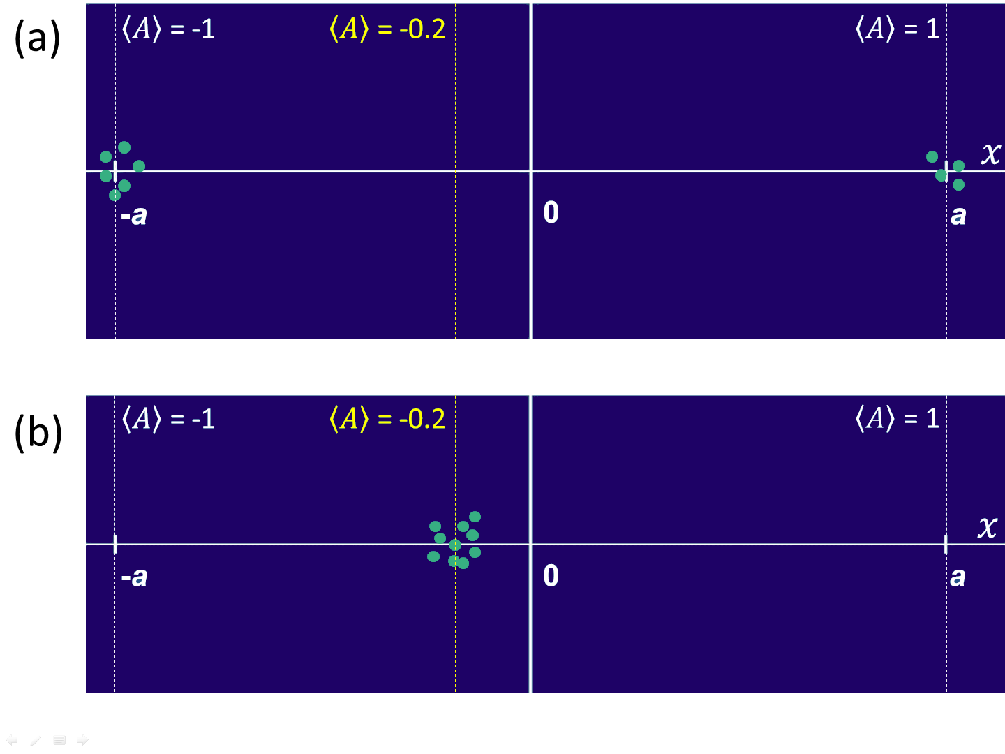
Figure 1: Theoretical framework (ideal pictorial representation). (a) Projective measurement: the two polarization components are completely separated, with the single photons impinging on two regions of the detector corresponding to the polarization operator eigenvaulues $A=\pm 1$. The expectation value $\expectationvalue*{A}$ is evaluated as the weighted average of the events, following Eq. (8). (b) Protective measurements: all the photons fall in the same region, centered in a position proportional to the polarization expectation value (see Eq. (9)).

II.1 Experimental Setup

Our experimental setup (Fig. 2) is divided in three parts.

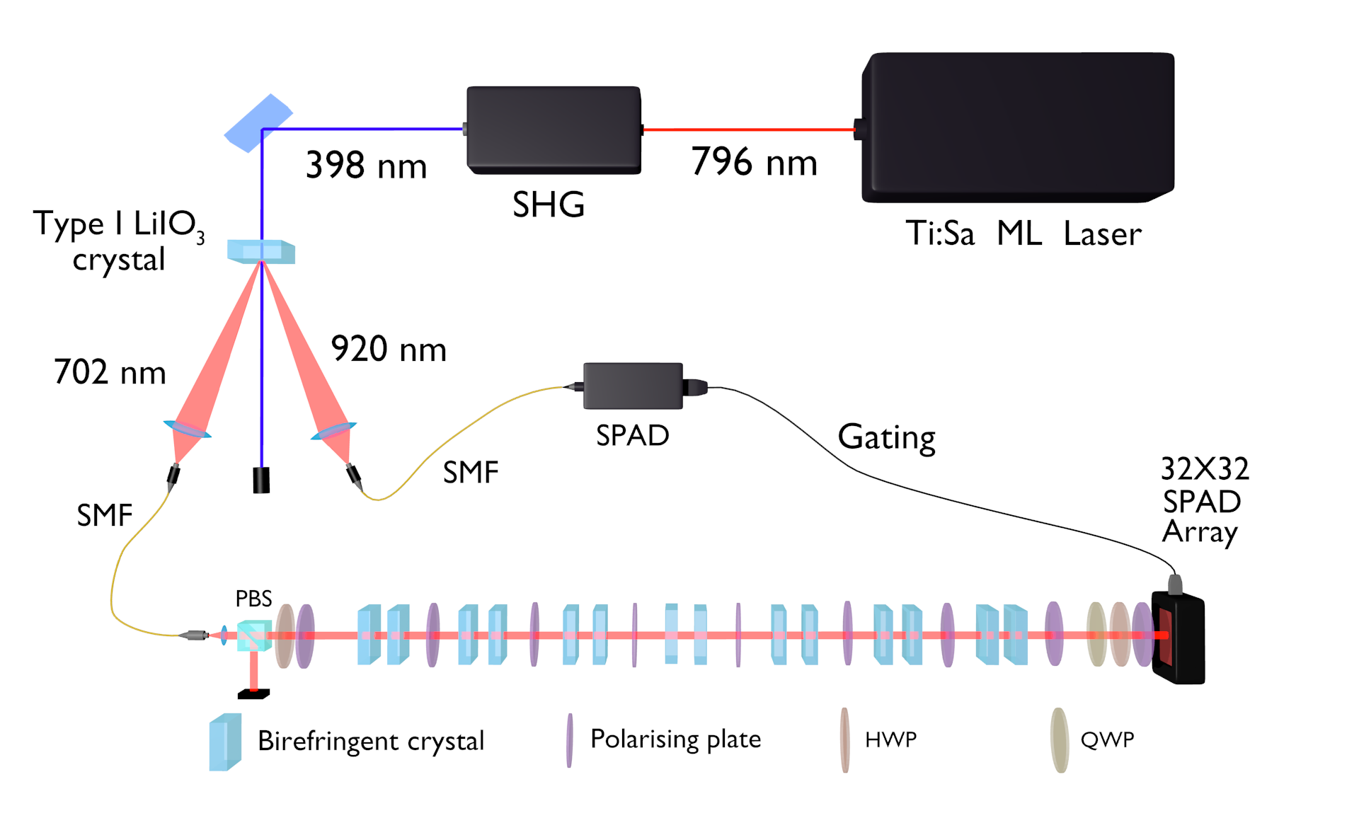
Figure 2: Experimental setup. SHG: second harmonic generator; SPAD: single-photon avalanche diode; SMF: single-mode fiber. HWP: half-wave plate. QWP: quarter-wave plate. PBS: polarising beam splitter. Ti:Sa ML laser: titanium-sapphire mode-locked laser.

In the first part, single photons are generated by a heralded single-photon source [81, 82]. A mode-locked laser with a second harmonic at 398 nm and a 76 MHz repetition rate pumps a $10\times 10\times 5$ mm LiIO₃ non-linear crystal, producing signal-idler photon pairs by exploiting Type-I spontaneous parametric down-conversion (SPDC). The generated idler photons (920 nm) are filtered by an interference filter (IF) centred at 920 nm and with a FWHM of 10 nm, and coupled to a single-mode fibre (SMF) which addresses them to a Silicon single-photon avalanche diode (SPAD), heralding the presence of the correlated signal photons (702 nm). Signal photons are filtered with an IF centred at 702 nm and with a FWHM of 10 nm, fibre-coupled and addressed to the second part of the setup, where the PM takes place. A Hanbury-Brown and Twiss interferometer allowed us to estimate the quality of our single-photon emission by evaluating the $\alpha$ parameter [83, 84], obtaining a value of $\alpha=0.13(1)$ without any background or dark count subtraction, testifying the high quality of our heralded single-photon source.
In the second part, the protective and projective measurements are performed. The signal photon produced in the previous stage is decoupled and collimated in a Gaussian spatial mode over a 2 m length. Then, it is initialized (pre-selected) in the polarization state $\ket{\psi}$ by a polarizing beam splitter (PBS) followed by a half-wave plate (HWP). Finally, in the projective measurement configuration the photon goes through $K=7$ weak interaction units (we chose the number of units $K=7$ from practical considerations approximating the ideal case of large $K$). Each unit consists of a first 2 mm long birefringent calcite crystal with an extraordinary ($e$) optical axis lying in the $x$ - $z$ plane, having an angle of $\pi/4$ with respect to the $z$ direction, followed by a second 1.1 mm calcite crystal with the optical $e$-axis oriented along the $y$-axis. The first crystal shifts the horizontally-polarized component of the wavefunction along the transverse direction $x$, while the second one compensates for the phase and time decoherence induced by the first crystal. The combined effect of all the 7 units allows for complete separation of orthogonal polarizations, reproducing the projective measurement framework. In the PM scenario, instead, the protection of the quantum state is implemented exploiting the quantum Zeno effect, realized by inserting a polarizing plate after each weak interaction unit. The polarizing plate realizes the projection $\Pi_{\psi}=\outerproduct{\psi}{\psi}$, projecting the state outgoing the weak von Neumann interaction onto the same polarization of the initial state $\ket{\psi}$, thus cancelling the (tiny) decoherence induced by the birefringent crystals in each weak interaction unit.

The final part of the experimental setup is the detection stage: photons are detected by a 2D spatial-resolving single-photon detector prototype, i.e. a two-dimensional array of 32x32 “smart pixels”, each hosting a SPAD with dedicated front-end electronics [85]. The detection of the idler photon (920 nm) by the Si-SPAD on the heralding arm gates the SPAD array with a 6 ns detection window. Furthermore, an optional quantum tomography [86, 87] apparatus, comprising a HWP, a quarter-wave plate (QWP) and a polarizer, can be inserted before the SPAD array to reconstruct the density matrix of the single-photon state at the end of each measurement procedure.

III Results

We acquired data sets for three different states: the state $\ket{+}=\frac{1}{\sqrt{2}}(\ket{H}+\ket{V})$, which should be subjected to the maximum decoherence, and two intermediate states $\ket{\frac{17}{60}\pi}=\cos(\frac{17}{60}\pi)\ket{H}+\sin(\frac{17}{60}\pi)\ket{V}$ and $\ket{\frac{\pi}{8}}=\cos(\frac{\pi}{8})\ket{H}+\sin(\frac{\pi}{8})\ket{V}$. Each data set is composed of multiple acquisitions:

• An acquisition with only the crystals in the optical path and $\ket{\psi}=\ket{H}$ or $\ket{\psi}=\ket{V}$, which allows us to calibrate the system.

• An acquisition without protection (only crystals in the optical path), corresponding to the traditional projective measurement scenario.

• An acquisition with both weak interaction and active Zeno-like protection (both birefringent crystals and polarisers in the optical path), realizing the PM.

• Two acquisitions, one with only the polarizing plates and one with a free optical path, allowing to complete the system calibration by evaluating and properly subtracting unwanted position biases introduced by crystals and polarizing plates.

III.1 Output state verification

To immediately highlight the difference between PM and projective (PJ) measurements, we perform a tomographic reconstruction of the states at the end of the measurement process.
In the PJ case, we expect that the repeated shifts of the horizontal polarization component cause decoherence on $\hat{\rho}_{in}=\outerproduct{\psi}{\psi}$, generating a final state $\hat{\rho}_{dec}$. On the contrary, in the PM case the protection should be able to preserve, in principle, the initial polarization state $\hat{\rho}_{in}$, thus we expect a final state $\hat{\rho}_{prot}=\hat{\rho}_{in}$:

$$\hat{\rho}_{in} =\begin{pmatrix}\cos^{2}(\theta)&-\sin(\theta)\cos(\theta)\\ \sin(\theta)\cos^{(}\theta)&\sin^{2}(\theta)\end{pmatrix}$$ (10)

$$\hat{\rho}_{dec} =\begin{pmatrix}\cos^{2}(\theta)&-\sin(\theta)\cos(\theta)\exp\left(-\frac{g^{\prime^{2}}}{(2\sigma)^{2}}\right)\\ \sin(\theta)\cos(\theta)\exp\left(-\frac{g^{\prime^{2}}}{(2\sigma)^{2}}\right)&\sin^{2}(\theta)\end{pmatrix}$$ (11)

where $g^{\prime}=\expectationvalue*{x_{H}}-\expectationvalue*{x_{V}}=11.56(7)$ px (pixels), being $\expectationvalue*{x_{H(V)}}$ the average position of photons in the $H(V)$ polarization on the $x$ axis, and $\sigma=4.17(2)$ px is the distribution width obtained by Gaussian fits.

We first compute the distance between the reconstructed states $\rho_{PM}^{rec}$ and $\rho_{PJ}^{rec}$, respectively obtained in the protective and projective measurement case (shown in Figure 3 for the state $\ket{\frac{17}{60}\pi}$), and their theoretical counterparts $\rho_{in}$ and $\rho_{dec}$, by evaluating the Fidelity $F$ [88, 89] between them (second and third columns of Table 1). The high Fidelities obtained certify the adherence of the experimental results to our model, showing that PM indeed preserves the initial state by the decoherence induced by the birefringent crystals, while this does not happen for projective measurements.

Then, we compute the distance between the two reconstructed states (fourth column of Table 1). Again, the low fidelities obtained tell us that, without protection, the decoherence induced on the initial state by the $K=7$ unitary interactions makes the final state totally incompatible with the one outgoing the PM procedure (and, obviously, with the initial state itself).

Finally, by analysing the purity $\mathcal{P}$ [88] of the reconstructed states (last two columns of Table 1), we notice that, as expected, the decoherence reduced the purity of the initial state $\rho_{in}$ in the PJ case, while this does not happen in the PM one. Thus, we have proved the PM protocol ability to preserve the coherence of the initial state during the whole measurement process, a feature in sharp contrast with the traditional quantum measurement paradigms.

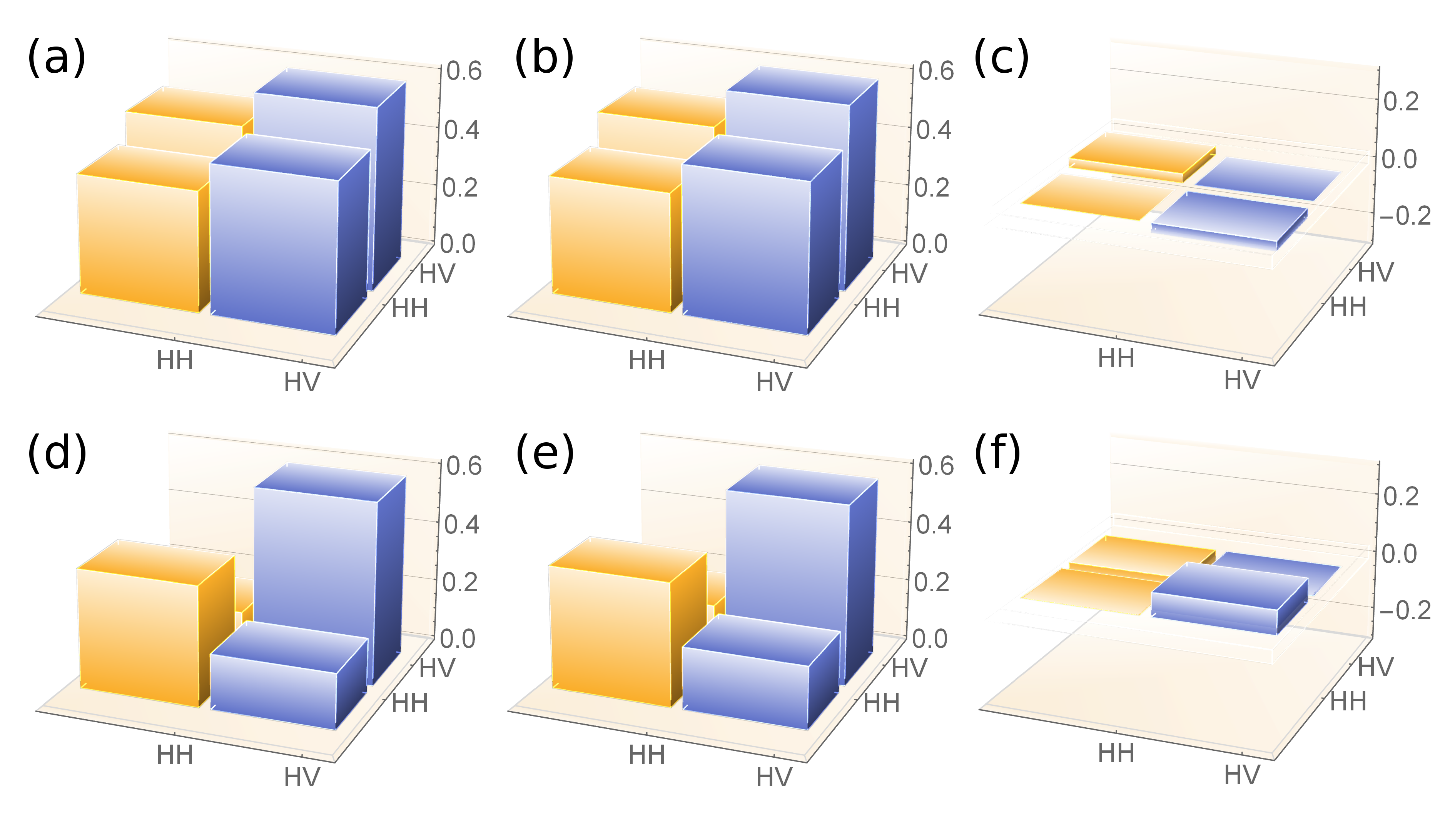
Figure 3: Density matrix reconstructions for the state outgoing the measurement process, considering an initial polarization state $\ket{\frac{17}{60}\pi}$: (a) Theoretical real part $\real[\rho_{in}]$ of the initial state density matrix ($\imaginary[\rho_{in}]=0$). (b) and (c), respectively: reconstructed real ($\real[\rho_{PM}^{rec}]$) and imaginary ($\imaginary[\rho_{PM}^{rec}]$) part of the density matrix of the single-photon state after the protective measurement. (d) theoretically-expected real part $\real[\rho_{dec}]$ of the density matrix of our state at the end of the projective measurement ($\imaginary[\rho_{dec}]=0$). (e) and (f), respectively: reconstructed real ($\real[\rho_{PJ}^{rec}]$) and imaginary ($\imaginary[\rho_{PJ}^{rec}]$) part of the density matrix of the single-photon state after undergoing the projective measurement.

Table 1: Comparison between theoretical and reconstructed density matrices. $F(\rho_{PM}^{rec},\rho_{in})$ and $F(\rho_{PJ}^{rec},\rho_{dec})$: Fidelities between reconstructed density matrices $\rho_{PM(PJ)}^{rec}$ and their theoretical counterparts $\rho_{in(dec)}$ in the PM (PJ) case. $F(\rho_{PM}^{rec},\rho_{PJ}^{rec})$: Fidelities between reconstructed protected and unprotected states. $\mathcal{P}(\rho_{PM}^{rec})$ and $\mathcal{P}(\rho_{PJ}^{rec})$: Purities of the reconstructed states in the PM and PJ case, respectively.

State	$F(\rho_{PM}^{rec},\rho_{in})$	$F(\rho_{PJ}^{rec},\rho_{dec})$	$F(\rho_{PM}^{rec},\rho_{PJ}^{rec})$	$\mathcal{P}(\rho_{PM}^{rec})$	$\mathcal{P}(\rho_{PJ}^{rec})$
$\ket{+}$	0.999	0.998	0.720	0.998	0.540
$\ket{\frac{17}{60}\pi}$	0.996	0.999	0.751	0.992	0.520
$\ket{\frac{\pi}{8}}$	0.992	0.999	0.894	0.992	0.789

III.2 Expectation values

Subsequently, in order to test the predictions of PM regarding the possibility of extracting the expectation value $\expectationvalue*{A}$ even from a single detection event, we evaluate $\expectationvalue*{A}$ with both the PM and PJ methods.

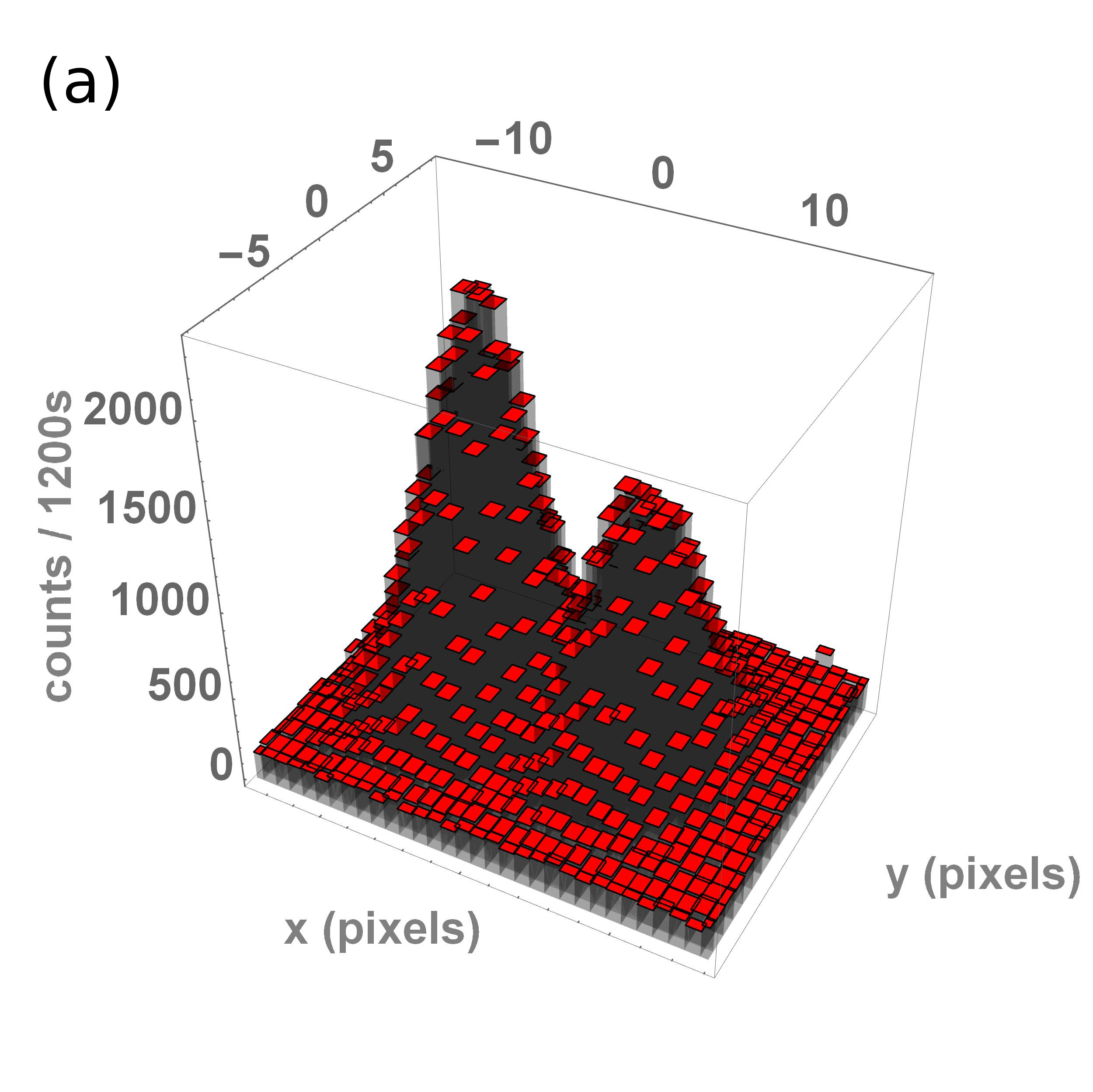
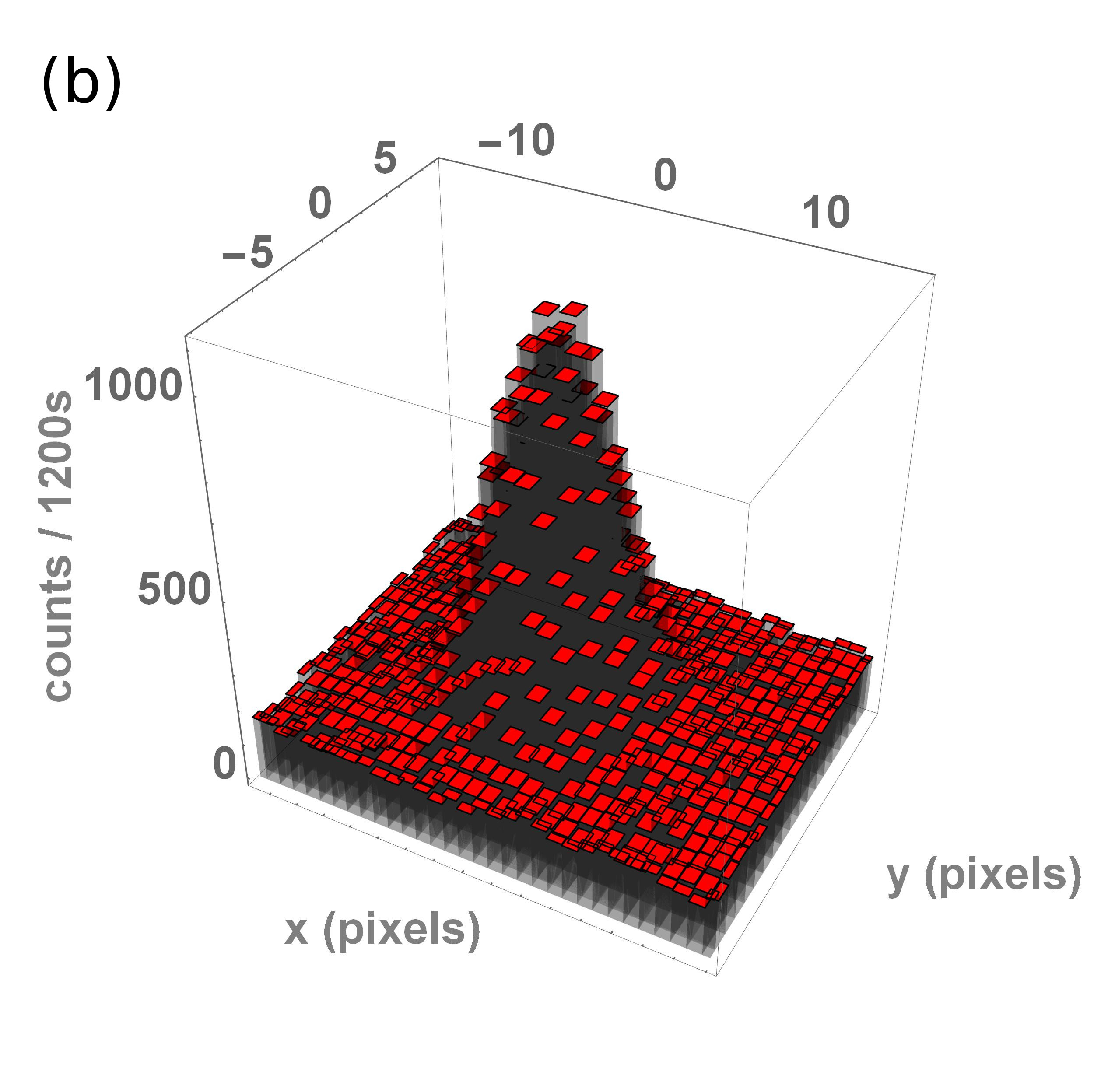
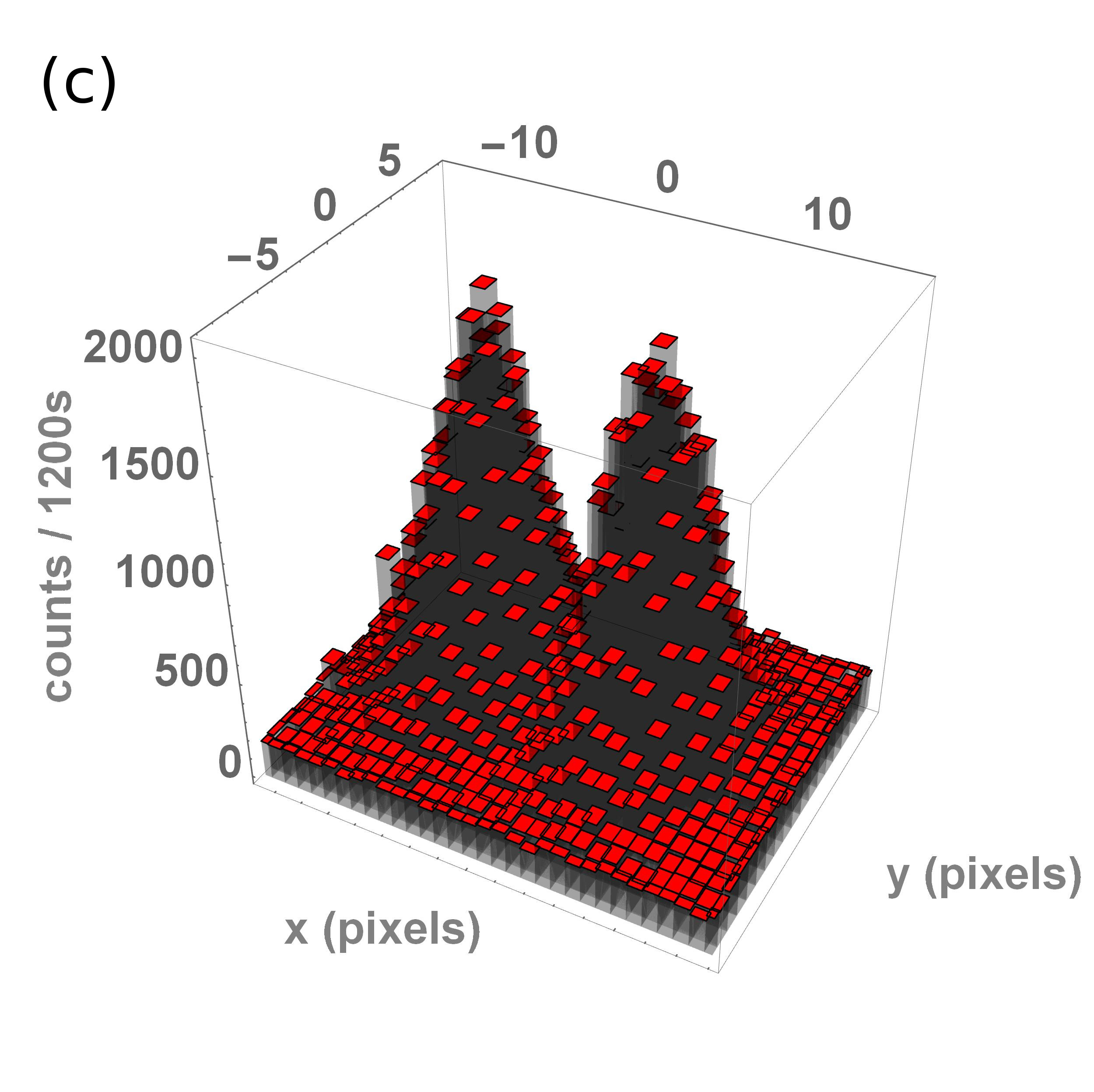
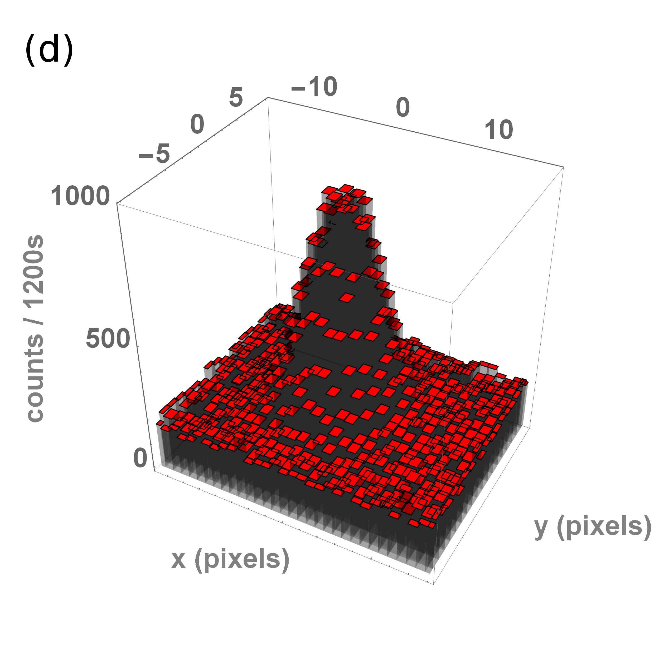
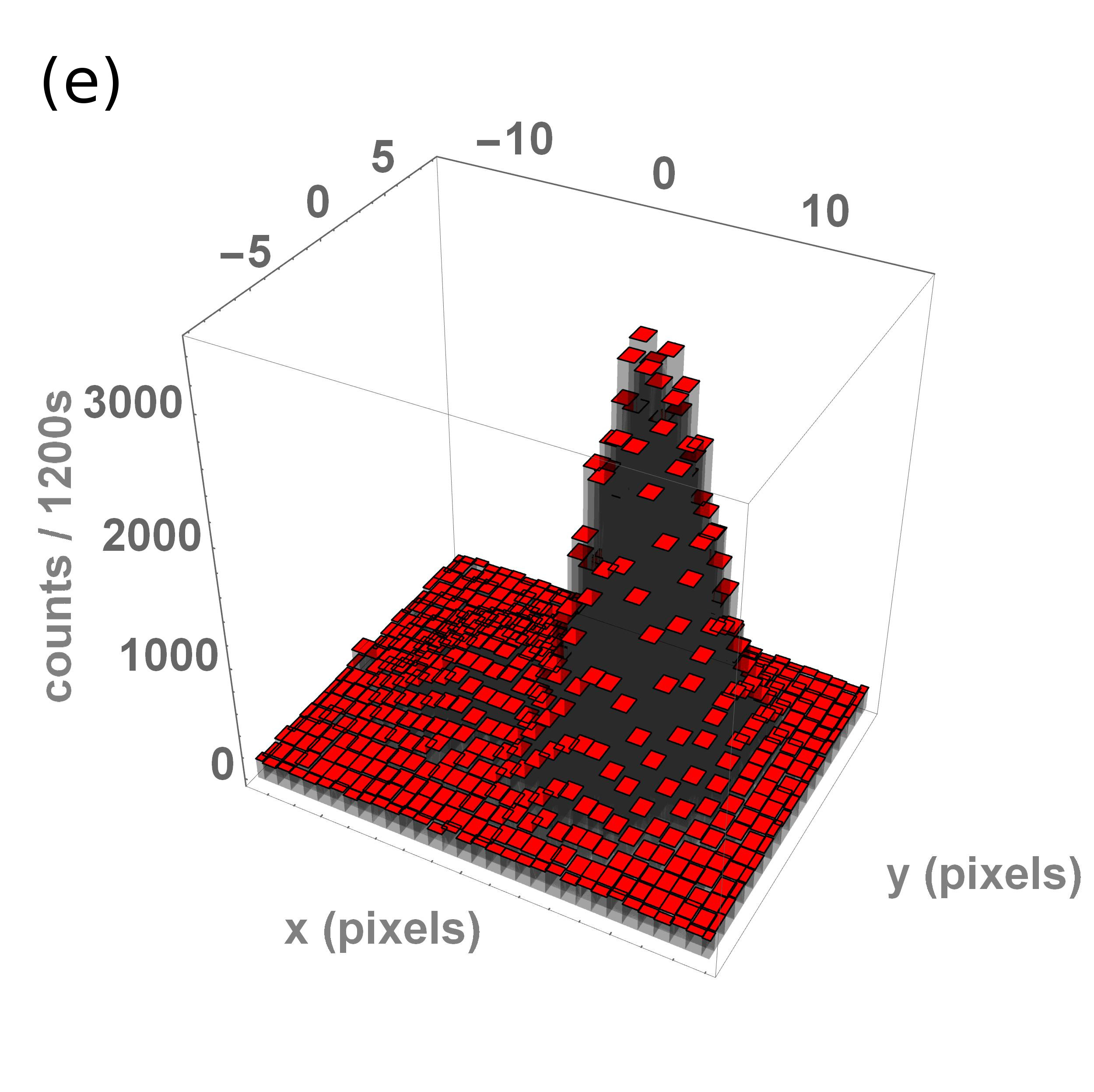
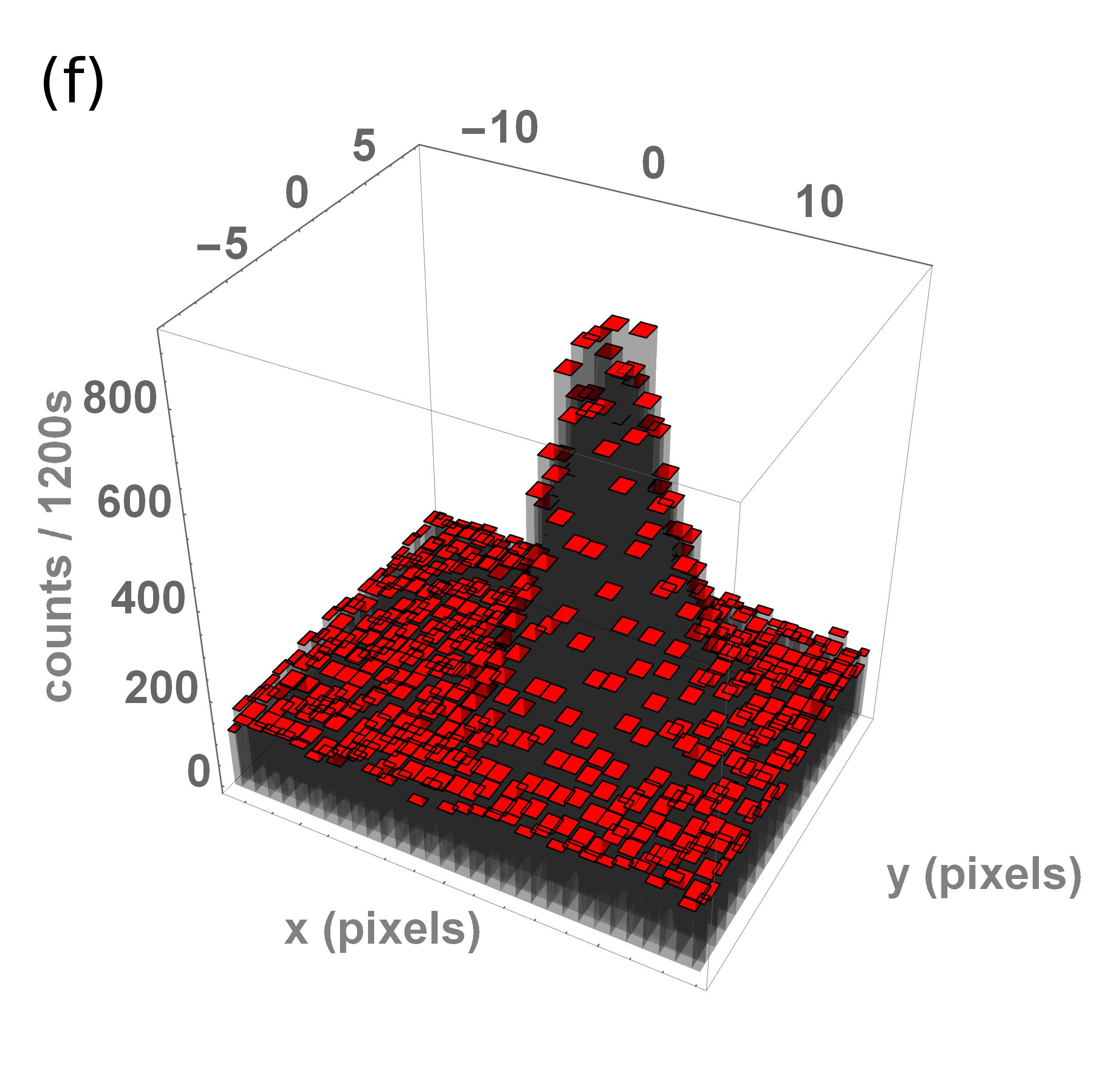
Figure 4: Plots of the photon counts distributions obtained with projective (a,c,d) and protective (b,d,f) measurements, for three different linearly-polarized initial states $\ket{\psi_{\theta}}$. a-b: ${\ket{\psi_{\frac{17}{60}\pi}}\approx 0.629\ket{H}+0.777\ket{V}}$; c-d: ${\ket{\psi_{\frac{\pi}{4}}}\approx 0.707\ket{H}+0.707\ket{V}}$; e-f: ${\ket{\psi_{\frac{\pi}{8}}}\approx 0.924\ket{H}+0.383\ket{V}}$.

Plots 4a, 4c, 4e show the results obtained for the three states in the PJ case. We can see that the photons accumulate around the two eigenvalues positions $x_{H}$ and $x_{V}$, hence we can statistically find the expectation value as the counts ratio in Eq. (8).

Plots 4b, 4d, 4f host, instead, the PM results, in which all the photons accumulate in a specific position corresponding to $x=a\expectationvalue*{A}$, in agreement with our expectations. This is clear evidence that, with protective measurements, each single photon carries information about the expectation value of its polarization.

The extracted expectation values are reported in Table 2, column 3 for PJ and in Table 2, column 4 for PM. A detailed description of the expectation values and uncertainties analysis can be found in Appendix A. We notice that the expectation values extracted with the PM method are in excellent agreement with the ones obtained with the traditional (PJ) one, as well as with the theoretically-expected values.

Table 2: Comparison between experimental and theoretical expectation values. Experimental expectation values. $\expectationvalue*{A}^{\mathrm{th}}$: theoretical expectation value. $\expectationvalue*{A}^{\mathrm{PJ}}$: experimental expectation value with projective measurements. $\expectationvalue*{A}^{\mathrm{PM}}$: experimental expectation value with protective measurements.

State	$\expectationvalue*{A}^{\mathrm{th}}$	$\expectationvalue*{A}^{\mathrm{PJ}}$	$\expectationvalue*{A}^{\mathrm{PM}}$
$\ket{+}$	0	-0.03(4)	0.0012(14)
$\ket{\frac{17}{60}\pi}$	-0.208	-0.21(2)	-0.19(2)
$\ket{\frac{\pi}{8}}$	0.707	0.72(2)	0.72(2)

To further confirm this result, the two plots in Fig. 5 show the equivalent of the distributions in Figs. 4a and 4b for few detection events. While, for the PM in Fig. 5b, all the counts (except for dark counts) belong to a region centered in the $x$ axis position corresponding to the expectation value $\expectationvalue*{A}$, the same does not happen for the PJ in Fig. 5a. Henceforth, with PM one can achieve a sound estimate of the average polarization value for the state $\ket{\frac{17}{60}\pi}$ from just the first detection event (yellow pixel in Fig. 5b), obtaining $\expectationvalue*{A}=-0.3\pm 0.3$, where the uncertainty is estimated from the width of the initial (Gaussian) spatial photon distribution. This result is in agreement with the theoretically-expected value $\expectationvalue*{A}^{\mathrm{th}}=-0.208$. On the contrary, it is not possible to do the same in the projective measurement case, since the first detection event (yellow pixel in Fig. 5a) does not provide any reliable information about the expectation value of the detected photon polarization. This is a final demonstration of the PM capability of extracting the expectation value even from a single detection event.

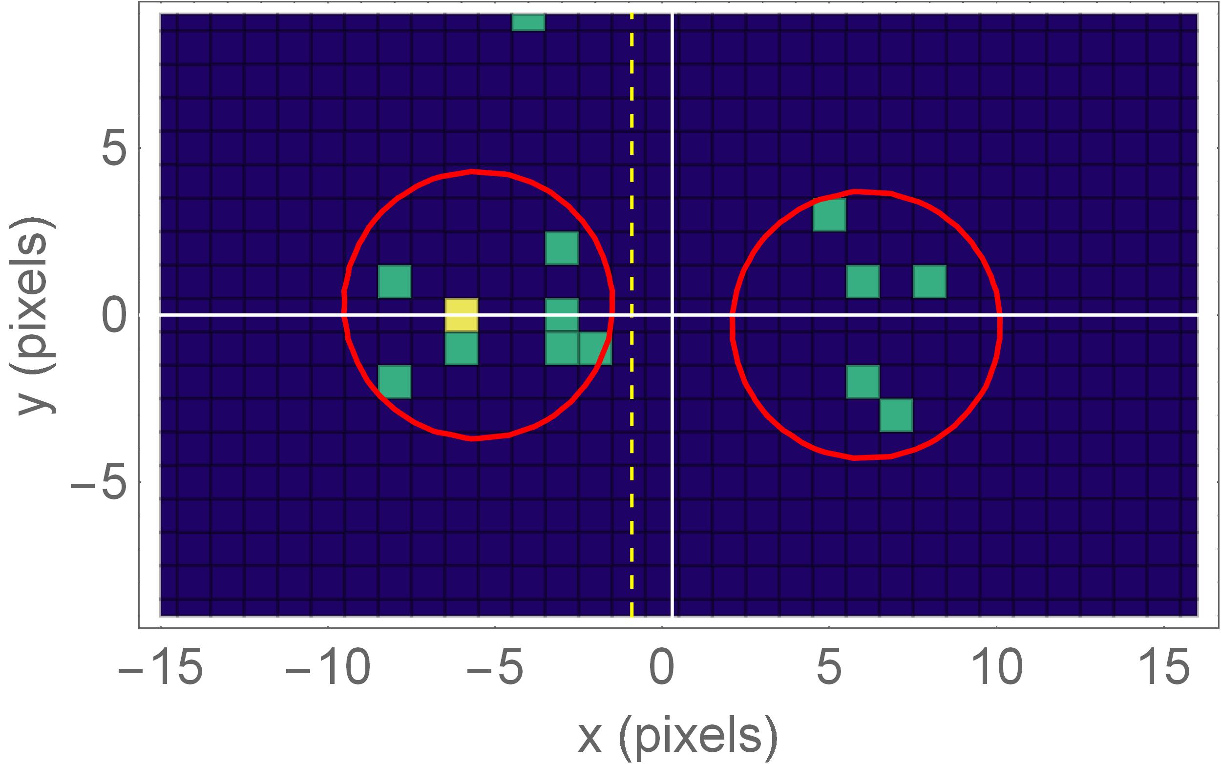
(a) Projective measurement case (14 detection events).

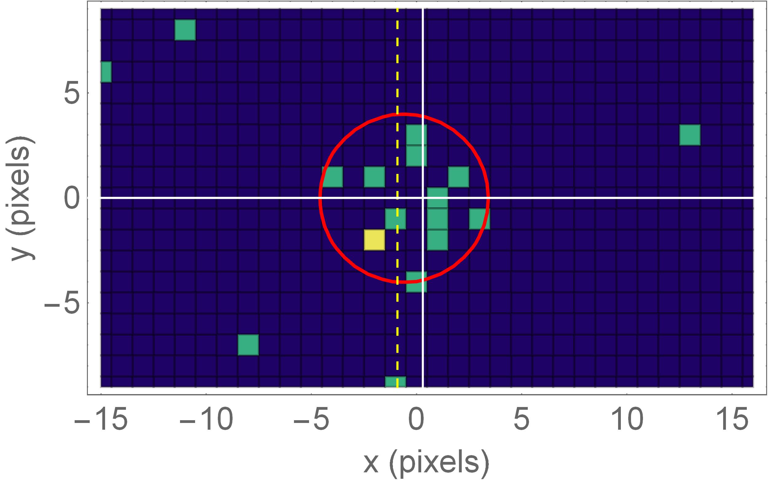
(b) Protective measurement (17 detection events).

Figure 5: Few-event photon counts distributions for the input state $\ket{\frac{17}{60}\pi}$, with the first detection event is marked in yellow. Yellow dashed line: $x$ position corresponding to the theoretical expectation value of the polarization $\expectationvalue*{A}^{\mathrm{th}}=-0.208$. Red circles: FWHM of the corresponding distributions for the state $\ket{\frac{17}{60}\pi}$ reported in Fig. 4.

IV Conclusions

Protective measurements represent a novel, groundbreaking measurement paradigm, which allows preserving the initial coherence of the measured state and extracting the expectation value of an observable, so far considered as a purely statistical quantity, even from a single detection event. The presented results demonstrate this unprecedented capability by exploiting certified single photons. In particular, in this paper we have described in detail the first experimental implementation of PM, providing the readers with all the details needed for a full understanding of the experiment and obtained results, as well as of the related implications for quantum mechanics foundations. We verified that PM preserves the coherence of the initial state during the whole measurement process, as certified by the high Fidelities between the initially-prepared states and the reconstructed ones outgoing the PM. Furthermore, the ability of PM to extract the expectation value of a quantum observable from a single (protected) particle is demonstrated by the photon distributions obtained with this protocol, always centered in a position proportional to the expectation value of the polarization of the detected photons and allowing to estimate polarization expectation values always in agreement with the ones obtained with traditional projective measurements, all matching the theoretical expectations within the experimental uncertainties.
These results shed important insight on the very foundations of quantum mechanics, especially in the long-standing debate about the ontic or epistemic nature of the wavefunction, at the same time paving the way toward new quantum measurement methods with possible significant application to quantum technologies and, in particular, to quantum metrology[90, 91, 92], with the eventual possibility to exceed the quantum Cramér-Rao bound [93] thanks to parameter dependence of the measurement procedure [94, 95] .

Author contributions

Conceptualization, E.C., I.P.D., L.V., M.Gen. and M.Gram.; methodology, A.A., E.C., F.P., I.P.D., L.V., M.Gen. and M.Gram.; software, A.A., E.R., F.P., I.P.D., R.L.; validation, I.P.D. and M.Gram.; formal analysis, E.R.; investigation, A.A., E.R. F.P.; resources, A.T., F.V., R.L.; data curation, F.P.; writing–original draft preparation, all authors; writing–review and editing, all authors; visualization, A.A., E.R. and F.P.; supervision, I.P.D., G.B., M.Gram. and M.Gen.; project administration, L.V. and M.Gen.; funding acquisition, E.C., I.P.D., M.Gen. and L.V. All authors have read and agreed to the published version of the manuscript.

Appendix: expectation value analysis

Here we describe more in detail our analysis of the expectation values in this work. The first step consists of extracting the centres $x_{H}$ and $x_{V}$ of the photon distributions corresponding to the horizontally- and vertically-polarized photons (i.e. the points corresponding to the $A$ eigenvalues $\pm 1$), respectively. This can be done by performing a linear regression of the acquisition for the states $\ket{H}$ and $\ket{V}$ and averaging over multiple acquisitions.

From the extracted $x_{H}$ and $x_{V}$, we define the center of our “laboratory system” (i.e. the point at $\expectationvalue*{A}=0$) as:

$$x_{0}=\frac{x_{H}+x_{V}}{2}$$ (12)

and the distance between the center and one of the two extremes as:

$$a=\frac{x_{H}-x_{V}}{2}$$ (13)

with an associated uncertainty of

$$\sigma_{a}=\sigma_{x_{0}}=\frac{\sqrt{\sigma^{2}_{x_{H}}+\sigma^{2}_{x_{V}}}}{2}$$ (14)

This allows evaluating the expectation values from both measurement procedures.

IV.1 Projective measurements

In the projective measurement case, we find the expectation value as the counts ratio:

$$\expectationvalue*{A}=\frac{(N_{H}-N_{H}^{(dark)})-(N_{V}-N_{V}^{(dark)})}{N_{H}+N_{V}-N_{H}^{(dark)}-N_{V}^{(dark)}}$$ (15)

where $N_{\mathrm{V(H)}}$ is the number of counts in the region corresponding to the vertical (horizontal) polarization component and $N_{\mathrm{V(H)}}^{(dark)}$ is the number of dark and background counts in the same region, estimated by evaluating the number of counts outside the region of interest of the detector.

The associated uncertainty is

$$\sigma_{\expectationvalue*{A}}=\sqrt{\sum_{k=1}^{4}\left(\partialderivative{A}{N_{k}}\right)^{2}\sigma_{N_{k}}^{2}}$$ (16)

with $N_{1}=N_{V}$, $N_{2}=N_{H}$, $N_{3}=N_{V}^{(dark)}$, $N_{4}=N_{H}^{(dark)}$. We evaluate the uncertainties on the number of background counts $N_{\mathrm{V(H)}}^{(dark)}$ by assuming a poissonian behaviour (i.e. $\sigma_{N_{V(H)}^{(dark)}}=\sqrt{N_{V(H)}^{(dark)}}$). The uncertainty on the number of photons in the two regions, instead, is more delicate, as the two distributions belonging to horizontally- and vertically-polarized photons are separated, but not completely. For this reason, we evaluate these uncertainties as

$$\sigma_{N_{H}} =\sqrt{N_{H}+(c_{H}\ N_{H})^{2}+(c_{V}\ N_{V})^{2}}$$ (17)

$$\sigma_{N_{V}} =\sqrt{N_{V}+(c_{H}\ N_{H})^{2}+(c_{V}\ N_{V})^{2}}$$ (18)

where the two coefficients $c_{\mathrm{H}}$ and $x_{\mathrm{V}}$ come from an ad hoc evaluation of the influence of the distribution tails (small, but still relevant) on the number of photon counts.

IV.2 Protective measurements

In the protective measurement case, each photon carries information about the expectation value, estimated as the ratio:

$$\expectationvalue*{A}=\frac{x-x_{0}}{a}$$ (19)

being $x$ the position of the photon, corrected by compensating for unwanted deviations induced by the polarizers and $a=g/2$. We extract $x$ from every pixel and then average it, weighting on the number of counts for each pixel. The associated uncertainty is

$$\sigma_{\expectationvalue*{A}}=\Bigg{[}\sigma_{\mathrm{ave}}+\left(\frac{1}{x_{H}^{\prime}-x_{V}^{\prime}}+\frac{\expectationvalue*{\hat{A}}}{x_{H}^{\prime}-x_{V}^{\prime}}\right)^{2}\sigma_{x_{H}^{\prime}}^{2}+\left(\frac{1}{x_{H}^{\prime}-x_{V}^{\prime}}-\frac{\expectationvalue*{\hat{A}}}{x_{H}^{\prime}-x_{V}^{\prime}}\right)^{2}\sigma_{x_{V}^{\prime}}^{2}\Bigg{]}^{1/2}$$ (20)

where $\sigma_{\mathrm{ave}}$ indicates the standard deviation of the mean of $\expectationvalue*{A}$. The second and third terms are the uncertainties on the parameters $x_{H(V)}^{\prime}=x_{H(V)}+x_{pol}-x_{void}$, where $x_{void}$ and $x_{pol}$ are the positions of the beam in the acquisition with a free optical path and with only the polarisers inserted, respectively. This allows us to compensate for the aforementioned unwanted polarisers-induced deviations. The variances associated with these parameters are $\sigma_{x_{H(V)}^{\prime}}^{2}=\sigma_{x_{H(V)}}^{2}+\sigma_{x_{pol}}^{2}+\sigma_{x_{void}}^{2}$.

References

- [1] Aharonov, Y.; Albert, D.Z.; and Vaidman, L. How the result of a measurement of a component of the spin of a spin-1/2 particle can turn out to be 100. Phys. Rev. Lett. 1988 60, 14, 1351-1354.
- [2] Tamir, B.; and Cohen, E. Introduction to weak measurements and weak values. Quanta 2013 2, 1, 7-17.
- [3] Aharonov, Y.; Vaidman, L. Measurement of the Schrödinger wave of a single particle. Phys. Lett. A 1993 178, 1, 38-42.
- [4] Aharonov, Y.; Anandan, J.; Vaidman, L. The Meaning of Protective Measurements. Found. Phys. 1996 26, 117-126.
- [5] Vaidman, L. Protective measurements. In Compendium of Quantum Physics; Greenberger, D. ; Hentschel, K.; Weinert, F., Ed. Springer: Berlin, Germany, 2009; pp 505-508.
- [6] Vaidman, L. Protective measurements. In Protective Measurement and Quantum Reality; Gao, S., Ed. Cambridge University Press: Cambridge, UK, 2014; pp 15-27.
- [7] Georgiev, D.; Cohen, E. Analysis of single-particle nonlocality through the prism of weak measurements. Int. J. Quantum Inf. 2020 18, 01, 1941024.
- [8] Ritchie, N.; Story, J.; Hulet, R. Realization of a measurement of a “weak value”. Phys. Rev. Lett. 1991 66, 9, 1107-1110.
- [9] Hosten, O.; Kwiat, P. Observation of the Spin Hall Effect of Light via Weak Measurements. Science 2008 319, 5864, 787-790
- [10] Dixon, P.; Starling, D.; Jordan, A.; Howell, J. Ultrasensitive Beam Deflection Measurement via Interferometric Weak Value Amplification. Phys. Rev. Lett. 2009 102, 173601.
- [11] Xu, X.; Kedem, Y.; Sun, K.; Vaidman, L.; Li, C.; Guo, G. Phase Estimation with Weak Measurement Using a White Light Source. Phys. Rev. Lett. 2013 111, 033604.
- [12] Piacentini, F.; Avella, A.; Levi, M.P.; Lussana, R.; Villa, F.; Tosi, A.; Zappa, F.; Gramegna, M.; Brida, G.; Degiovanni, I.P.; Genovese, M. Experiment Investigating the Connection between Weak Values and Contextuality. Phys. Rev. Lett. 2016 116, 180401.
- [13] Cimini, V.; Gianani, I.; Piacentini, F.; Degiovanni, I.P.; Barbieri, M. Anomalous values, Fisher information, and contextuality, in generalized quantum measurements. Quantum Sci. Technol. 2020 5, 025007.
- [14] Lundeen, J.; Sutherland, B.; Patel, A.; Stewart, C.; Bamber, C. Direct measurement of the quantum wavefunction. Nature 2011 474, 188-191.
- [15] Goggin, M.; Almeida, M.P.; Barbieri, M.; Lanyon, B.P.; O’Brien, J.L.; White, A.G.; Pryde, G.J. Violation of the Leggett-Garg inequality with weak measurements of photons. Proc. Natl. Acad. Sci. USA 2011 108, 4, 1256-1261.
- [16] Magana Loaiza, O.; Mirhosseini, M.; Rodenburg, B.; Boyd, R. Amplification of Angular Rotations Using Weak Measurements. Phys. Rev. Lett. 2014 112, 200401.
- [17] Resch, K.J.; Steinberg, A.M. Extracting Joint Weak Values with Local, Single-Particle Measurements. Phys. Rev. Lett. 2004 92, 130402.
- [18] Hallaji, M.; Feizpour, A.; Dmochowski, G.; Sinclair, J.; Steinberg, A.M. Weak-value amplification of the nonlinear effect of a single photon. Nat. Phys. 2017 13, 540.
- [19] Avella, A.; Piacentini, F.; Borsarelli, M.; Barbieri, M.; Gramegna, M.; Lussana, R.; Villa, F.; Tosi, A.; Degiovanni, I.P.; Genovese, M. Anomalous weak values and the violation of a multiple-measurement Leggett-Garg inequality. Phys. Rev. A 2017 96, 052123.
- [20] Ferrie, C.; Combes, J. How the Result of a Single Coin Toss Can Turn Out to be 100 Heads. Phys. Rev. Lett. 2014 113, 120404.
- [21] Sinclair, J.; Spierings, D.; Brodutch, A.; Steinberg, A. Interpreting weak value amplification with a toy realist model. Phys. Lett. A 2019 383, 24, 2839-2845.
- [22] Mundarain, D.; Orszag, M. Quantumness of the anomalous weak measurement value. Phys. Rev. A 2016 93, 032106.
- [23] Mitchinson, G.; Jozsa, R.; Popescu, S. Sequential weak measurement. Phys. Rev. A 2007 76, 062105.
- [24] Piacentini, F.; Avella, A.; Levi, M.P.; Gramegna, M.; Brida, G.; Degiovanni, I.P.; Cohen, E.; Lussana, R.; Villa, F.; Tosi, A.; Zappa, F.; Genovese, M. Measuring Incompatible Observables by Exploiting Sequential Weak Values. Phys. Rev. Lett. 2016 117, 170402.
- [25] Thekkadath, G.S.; Giner, L.; Chalich, Y.; Horton, M.J.; Banker, J.; Lundeen, J.S. Direct Measurement of the Density Matrix of a Quantum System. Phys. Rev. Lett. 2016 117, 120401.
- [26] Kim, Y.; Kim, Y.-S.; Lee, S.-Y.; Han, S.-W.; Moon, S.; Kim, Y.-H.; Cho, Y.-W. Direct quantum process tomography via measuring sequential weak values of incompatible observables. Nat. Commun. 2018 9, 192.
- [27] Foletto, G.; Calderaro, L.; Tavakoli, A.; Schiavon, M.; Picciariello, F.; Cabello, A.; Villoresi, P.; Vallone, G. Experimental Certification of Sustained Entanglement and Nonlocality after Sequential Measurements. Phys. Rev. Applied 2020 13, 044008.
- [28] Foletto, G.; Calderaro, L.; Vallone, G.; Villoresi, P. Experimental demonstration of sequential quantum random access codes. Phys. Rev. Research 2020 2, 033205.
- [29] Foletto, G.; Padovan, M.; Avesani, M.; Tebyanian, H.; Villoresi, P.; Vallone, G. Experimental Test of Sequential Weak Measurements for Certified Quantum Randomness Extraction. arXiv:2101.12074 2021.
- [30] Salazar-Serrano, L.J.; Guzmán, D.A.; Valencia, A.; Torres, J.P. Demonstration of a highly-sensitive tunable beam displacer with no use of beam deflection based on the concept of weak value amplification. Opt. Expr. 2015 23, 8, 10097.
- [31] Calderón-Losada, O.; Moctezuma Quistian, T.T.; Cruz-Ramirez, H.; Murgueitio Ramirez, S.; U’Ren, A.B.; Botero, A.; Valencia, A. A weak values approach for testing simultaneous Einstein–Podolsky–Rosen elements of reality for non-commuting observables. Commun. Phys. 2020 3, 117.
- [32] Piacentini, F.; Avella, A.; Gramegna, M.; Lussana, R.; Villa, F.; Tosi, A.; Brida, G.; Degiovanni, I.P.; Genovese, M. Investigating the Effects of the Interaction Intensity in a Weak Measurement. Sci. Rep. 2018 8, 6959.
- [33] Pan, Y.; Zhang, J.; Cohen, E.; Wu, CW.; Chen, PX.; Davidson, N. Weak-to-strong transition of quantum measurement in a trapped-ion system. Nat. Phys. 2020 16, 1206–1210.
- [34] Pan, WW.; Xu, XY.; Kedem, Y.; Wang, QQ.; Chen, Z.; Jan, M.; Sun, K.; Xu, JS.; Han, YJ.; Li, CF.; Guo, GC. Direct Measurement of a Nonlocal Entangled Quantum State. Phys. Rev. Lett. 2019 123, 150402.
- [35] Cho, YW.; Kim, Y.; Choi, YH.; Kim, YS.; Han, SW.; Lee, SY. Moon, S.; Kim, YH. Emergence of the geometric phase from quantum measurement back-action. Nat. Phys. 2019 15, 665–670.
- [36] Shikano, Y.; Hosoya, A. Weak values with decoherence. J. Phys. A: Math. Theor. 2009 43, 025304.
- [37] Shikano, Y.; Hosoya, A. Strange weak values. J. Phys. A: Math. Theor. 2010 43, 385307.
- [38] Susa, Y.; Shikano, Y.; Hosoya, A. Optimal probe wave function of weak-value amplification. Phys. Rev. A 2012 85, 052110.
- [39] Kobayashi, H.; Puentes, G.; Shikano, Y. Extracting joint weak values from two-dimensional spatial displacements. Phys. Rev. A 2012 86, 053805.
- [40] Vaidman, L. Weak value controversy. Philos. Trans. R. Soc. A 2017 375, 2106.
- [41] Aharonov, Y.; Anandan, J.; Vaidman, L. Meaning of the wave function. Phys. Rev. A 1993 47, 6, 4616-4626.
- [42] Rovelli, C. Comment on “Meaning of the wave function”. Phys. Rev. A 1994 50, 2788-2792.
- [43] Unruh, W.G. Reality and measurement of the wave function. Phys. Rev. A 1994 50, 882-887.
- [44] Dickson, M. An empirical reply to empiricism: protective measurement opens the door for quantum realism. Philos. Sci. 1995 62, 122-140.
- [45] D’Ariano, G.M.; Yuen, H.P. Impossibility of measuring the wave function of a single quantum system. Phys. Rev. Lett. 1996 76, 2832-2835.
- [46] Dass, N.H.; Qureshi, T. Critique of protective measurements. Phys. Rev. A 1999 59, 2590-2601.
- [47] Uffink, J. How to protect the interpretation of the wave function against protective measurements. Phys. Rev. A 1999 60, 3474-3481.
- [48] Gao, S. On Uffink’s criticism of protective measurements. Stud. Hist. Philos. Sci. 2013 44, 513-518.
- [49] Genovese, M. Interpretations of quantum mechanics and measurement problem. Adv. Sci. Lett. 2010 3, 3, 249-258.
- [50] Pusey, M.F.; Barrett, J.; Rudolph, T. On the reality of the quantum state. Nat. Phys. 2012 8, 6, 475-478.
- [51] Hardy, L. Are quantum states real? Int. J. Mod. Phys. B 2013 27, 01n03, 1345012.
- [52] Ringbauer, M.; Duffus, B.; Branciard, C.; Cavalcanti, E.G.; White, A.G.; Fedrizzi, A. Measurements on the reality of the wavefunction. Nat. Phys. 2015 11, 3, 249-254.
- [53] Gao, S. Protective Measurement and Quantum Reality; Cambridge University Press: Cambridge, UK, 2015.
- [54] Gao, S. Protective Measurements and the Reality of the Wave Function. arxiv:2001.09262 2020.
- [55] Khrennikov, A. Emergence of Quantum Mechanics from Theory of Random Fields. J. Russ. Laser Res. 2017 38, 9-26.
- [56] Pan, A.K. Two definitions of maximally -epistemic ontological model and preparation non-contextuality. arXiv:2012.13881 2020.
- [57] Piacentini, F.; Avella, A.; Rebufello, E.; Lussana, R.; Villa, F.; Tosi, A.; Gramegna, M.; Brida, G.; Cohen, E.; Vaidman, L.; Degiovanni, I.P.; Genovese, M. Determining the quantum expectation value by measuring a single photon. Nat. Phys. 2017 13, 12, 1191–1194.
- [58] von Neumann, J. Mathematische Grundlagen der Quantenmechanik; Springer: Berlin, Germany, 1932.
- [59] Misra, B.; Sudarshan, E.C.G. The zeno’s paradox in quantum theory. J. Math. Phys. 1977 18, 4, 756-763.
- [60] Itano, W.M.; Heinzen, D.J.; Bollinger, J.J; Wineland. D.J. Quantum zeno effect. Phys. Rev. A 1990 41, 2295.
- [61] Kwiat, P.; Weinfurter, H.; Herzog, T.; Zeilinger, A.; Kasevich, M.A. Interaction-Free Measurement. Phys. Rev. Lett. 1995 74, 4763.
- [62] Kofman, A.G.; Kurizki, G. Quantum Zeno effect on atomic excitation decay in resonators. Phys. Rev. A 1996 54, R3750.
- [63] Kofman, A.G.; Kurizki, G. Acceleration of quantum decay processes by frequent observations. Nature 2000 405, 546.
- [64] Kofman, A.G.; Kurizki, G. Universal Dynamical Control of Quantum Mechanical Decay: Modulation of the Coupling to the Continuum. Phys. Rev. Lett. 2001 87, 270405.
- [65] Fischer, M.C.; Gutiérrez-Medina, B.; Raizen, M.G. Observation of the quantum Zeno and anti-Zeno effects in an unstable system. Phys. Rev. Lett. 2001 87, 040402.
- [66] Facchi, P.; Pascazio, S. Quantum zeno subspaces. Phys. Rev. Lett. 2002 89, 080401.
- [67] Facchi, P.; Pascazio, S. Quantum Zeno dynamics: mathematical and physical aspects. J. Phys. A 2008 41, 493001.
- [68] Smerzi, A. Zeno dynamics, indistinguishability of state, and entanglement. Phys. Rev. Lett. 2012 109, 150410.
- [69] Schäfer, F.; Herrera, I.; Cherukattil, S.; Lovecchio, C.; Cataliotti, F.S.; Caruso, F.; Smerzi, A. Experimental realization of quantum zeno dynamics. Nat. Commun. 2014 5, 3194.
- [70] Signoles, A.; Facon, A.; Grosso, D.; Dotsenko, I.; Haroche, S.; Raimond, J.-M.; Brune, M.; Gleyzes, S. Confined quantum Zeno dynamics of a watched atomic arrow. Nat. Phys. 2014 10, 715.
- [71] Gherardini, S.; Gupta, S.; Cataliotti, F.S.; Smerzi, A.; Caruso, F.; Ruffo, S. Stochastic quantum Zeno by large deviation theory. New J. Phys. 2016 18, 013048.
- [72] Müller, M.M.; Gherardini, G.; Caruso, F. Noise-robust quantum sensing via optimal multi-probe spectroscopy. Sci. Rep. 2016 6, 38650.
- [73] Gherardini, S.; Lovecchio, C.; Müller, M.M.; Lombardi, P.; Caruso, F.; Cataliotti, F.S. Ergodicity in randomly perturbed quantum systems. Quantum Sci. Technol. 2017 2, 015007.
- [74] Müller, M.M.; Gherardini, S.; Caruso, F. Quantum Zeno dynamics through stochastic protocols. Ann. Phys. 2017 529, 1600206.
- [75] Harel, G.; Kofman, A.G.; Kozhekin, A.; Kurizki, G. Control of non-Markovian decay and decoherence by measurements and interference. Opt. Express 1998 2, 355.
- [76] Gordon, G.; Erez, N.; Kurizki, G. Universal dynamical decoherence control of noisy single-and multi-qubit systems. J. Phys. B 2007 40, S75.
- [77] Kurizki, G.; Shahmoon, E.; Zwick, A. Thermal baths as quantum resources: morefriends than foes? Phys. Scr. 2015 90, 128002.
- [78] Elliott, T.J.; Vedral, V. Quantum quasi-Zeno dynamics: Transitions mediated by frequent projective measurements near the Zeno regime. Phys. Rev. A 2016 94, 012118.
- [79] Virzí, S.; et al. Quantum Zeno and Anti-Zeno probes of noise correlations in photon polarisation. arXiv:2103.03698, 2021.
- [80] Gerlach, W.; Stern, O. Der experimentelle nachweis der richtungsquantelung im magnetfeld. Z. Phys. 1922 9, 1, 349-352.
- [81] Eisaman, M.D.; Fan, J.; Migdall, A.; Polyakov, S.V. Single-photon sources and detectors. Rev. Scient. Instrum. 2011 82, 071101.
- [82] Sinha, U.; Sahoo, S. N.; Singh, A.; Joarder, K.; Chatterjee, R.; Chakraborti, S. Single-Photon Sources. Opt. Photonics News 2019 30, 9, 32-39 .
- [83] Grangier, P.; Roger, G.; Aspect, A. Experimental Evidence for a Photon Anticorrelation Effect on a Beam Splitter: A New Light on Single-Photon Interferences. EPL 1986 1, 4, 173-179.
- [84] Chunnilall, C.J.; Degiovanni, I.P.; Kück, S.; Müller, I.; Sinclair, A.G. Metrology of single-photon sources and detectors: a review. Opt. Eng. 2014 53, 8, 081910.
- [85] Villa, F.; Lussana, R.; Bronzi, D.; Tisa, S.; Tosi, A.; Zappa, F.; Dalla Mora, A.; Contini, D.; Durini, D.; Weyers, S.; Brockherde, W. Cmos imager with 1024 spads and tdcs for single-photon timing and 3-d time-of-flight. IEEE J. Sel. Top. Quantum Electron. 2014 20, 6, 364-373.
- [86] Altepeter, J.; Jeffrey, E.; Kwiat, P. Photonic state tomography. Vol. 52 of Advances In Atomic, Molecular, and Optical Physics; Berman, P.; Lin, C., Academic Press, Cambridge, MA, USA, 2005; pp. 105-159.
- [87] Bogdanov, Y.I.; Brida, G.; Genovese, M.; Kulik, S.P.; Moreva, E.V.; Shurupov, A.P. Statistical Estimation of the Efficiency of Quantum State Tomography Protocols. Phys. Rev. Lett. 2010 105, 010404.
- [88] Nielsen, M.; Chuang, I. Quantum Computation and Quantum Information; Cambridge University Press, Cambridge, UK, 2010.
- [89] Bengstonn, I.; Zyczkowski, K. Geometry of Quantum States; Cambridge University Press, Cambridge, UK,, 2008.
- [90] Giovannetti, V.; Lloyd, S.; Maccone, L. Advances in quantum metrology. Nat. Photon. 2011 5, 222–229.
- [91] Genovese, M. Experimental Quantum Enhanced Optical Interferometry. arXiv:2101.02891 2021.
- [92] Polino, E.; Valeri, M.; Spagnolo, N.; Sciarrino, F. Photonic Quantum Metrology. AVS Quantum Sci. 2020 2, 024703.
- [93] Paris, M. G. A. Quantum estimation for quantum technology. Int. J. of Quantum Inf. 7 2009 1, 125-137.
- [94] Seveso, L.; Rossi, M. A. C.; Paris, M. G. A. Quantum metrology beyond the quantum Cramér-Rao theorem. Phys. Rev. A 2017 95, 012111.
- [95] Seveso, L.; Paris, M. G. A. Quantum enhanced metrology of hamiltonian parameters beyond the Cramér-Rao bound. Int. J. of Quantum Inf. 2020 18, 3, 2030001.