Dynamically Modelling Heterogeneous Higher-Order Interactions for Malicious Behavior Detection in Event Logs

Abstract.

Anomaly detection in event logs is a promising approach for intrusion detection in enterprise networks. By building a statistical model of usual activity, it aims to detect multiple kinds of malicious behavior, including stealthy tactics, techniques and procedures (TTPs) designed to evade signature-based detection systems. However, finding suitable anomaly detection methods for event logs remains an important challenge. This results from the very complex, multi-faceted nature of the data: event logs are not only combinatorial, but also temporal and heterogeneous data, thus they fit poorly in most theoretical frameworks for anomaly detection. Most previous research focuses on one of these three aspects, building a simplified representation of the data that can be fed to standard anomaly detection algorithms. In contrast, we propose to simultaneously address all three of these characteristics through a specifically tailored statistical model. We introduce Decades, a dynamic, heterogeneous and combinatorial model for anomaly detection in event streams, and we demonstrate its effectiveness at detecting malicious behavior through experiments on a real dataset containing labelled red team activity. In particular, we empirically highlight the importance of handling the multiple characteristics of the data by comparing our model with state-of-the-art baselines relying on various data representations.

1. Introduction

Beyond rousing and slightly delusive forecasts of undefeatable AI-powered intrusion detection systems, anomalous activity detection in computer networks can be seen as the intersection of two main concepts. The first one is behavioral analysis, which could be defined as focusing on activity rather than static attributes – for instance, looking for processes repeatedly encrypting files in a short time span rather than executables matching known ransomware samples. The second one is anomaly detection, an approach aiming to characterize the benign rather than the malicious, defining the latter as ”not known good” instead of ”known bad”. A practical example is looking for unusual parent-child process associations rather than traces of a specific family of exploits. These two paradigms share a common goal: building more generic and robust detection methods, capable of spotting advanced attackers using stealthy tactics, techniques and procedures (TTPs) such as living-off-the-land or supply chain attacks. End goals of such threat actors include espionage, sabotage and financial gain.

In practice, behavioral models of computer networks are often built using event logs, which are basically records of various kinds of activity happening within a given perimeter. These logs can be generated either by hosts or network equipments. Being able to build a statistical model of events recorded inside a given network theoretically allows security experts to detect all kinds of malicious behaviors, as long as they are inconsistent with what usually happens in the computer network at hand. However, fully addressing the complexity of such data remains a major challenge. Indeed, let alone the sheer variety of benign and malicious behaviors that must be dealt with, event logs do not easily lend themselves to mathematical characterization. They are primarily combinatorial data, in that each event is defined by a finite number of fields mostly containing discrete values: user and host names, IP addresses, and so on. But there is also a temporal dimension: events appear at specific instants, and they result from activity that evolves over time. Finally, the multiplicity of actions occurring in a computer network makes event logs intrinsically heterogeneous: for instance, it hardly makes sense to compare an authentication and a process creation.

Due to this complexity, standard anomaly detection algorithms cannot be used as such on event logs: the significant semantic gap between the data and the model must be bridged. Most existing work circumvents this problem by adapting the data to the model, simplifying them enough to make them fit into a standard anomaly detection framework (Yen et al., 2013; Legg et al., 2015; Hu et al., 2017). This leads to significant information loss, in turn bounding the performance of the whole detection procedure: once relevant aspects of the data have been erased, even the smartest algorithm will be unable to recover them. Therefore, recent contributions have developed a more comprehensive approach, coming up with better suited models instead of oversimplifying the data (Tuor et al., 2018; Amin et al., 2019; Leichtnam et al., 2020). In particular, significant progress has been made towards adequately modelling the combinatorial dimension of events. Our work builds upon these recent advances, extending them to simultaneously address the temporal and heterogeneous aspects in addition to the combinatorial one.

We propose Decades, a dynamic, heterogeneous and combinatorial model for anomaly detection in event streams. This model can be used to learn the usual activity patterns in a computer network, subsequently identifying anomalies at the event granularity. We make use of multi-task learning to efficiently handle the heterogeneity of event logs, improving our model by jointly learning the behavior of entities across all event types. We also design a retraining strategy to track the evolution of the network and avoid concept drift, enabling fine-tuning of the balance between fitting to new data and remembering past information. Finally, we evaluate Decades against several state-of-the-art baselines and show its effectiveness on a real dataset containing labelled red team activity (Kent, 2015a).

The rest of this paper is structured as follows. We first give some basic definitions and review existing work in Section 2. The next two sections are devoted to describing our model: we address the combinatorial and heterogeneous dimensions in Section 3, and Section 4 deals with the updating procedure we use to handle temporal evolution of the data distribution. We present our experiments and results in Section 5. Finally, we discuss some limitations of Decades along with leads for future research in Section 6 and briefly conclude in Section 7.

2. Problem Formulation and Related Work

We start by defining some essential notions and formally stating the problem considered here, then review previous research addressing this problem.

2.1. Event Logs and Intrusion Detection – Formal Definitions

Consider a computer network, which we define here as a heterogeneous set of entities (e.g. users, hosts, files). Our interest lies in monitoring activity inside this network in order to detect malicious behavior (defined in more detail below). A wide variety of data sources can be used, mostly decomposing into two categories: host logs (e.g. Windows event logs) and network logs (e.g. NetFlows). In order to make our work applicable independently of the specific data source at hand, we use an abstract definition built upon the notion of event. An event is generically defined as an interaction between two or more entities, further characterized by a timestamp, an event type and some optional additional information. Authentications can for instance be represented as interactions between users and hosts, with additional information such as the authentication package used. Note that this representation is not unique: one could for example treat the authentication package as an involved entity rather than additional information, or include the source and destination hosts as two separate entities.

There are three important aspects in the above definition. First, events are combinatorial data, in that they are primarily defined as a combination of entities chosen from finite sets. But there are several event types, and the observed combinations of entities depend on the type: for instance, an authentication and a process creation involve different kinds of entities. In other words, event logs are intrinsically heterogeneous data. Finally, each event is associated with a specific timestamp, and the probability of observing a given event is not necessarily constant in time. This endows event logs with a temporal dimension. Although none of these three characteristics is new to the seasoned statistician, observing all three of them simultaneously is less frequent.

Given a sequence of events, intrusion detection consists in finding a subset of this sequence reflecting malicious activity. Here, we consider a continuous monitoring setting: we first use a set of supposedly benign historical events to infer the normal behavior of the system. We then observe a stream of new events and, using these events, we try to detect malicious activity as soon as possible when it happens. More specifically, we focus on post-compromise detection: we look for an attacker having already gained a foothold inside the network, trying to elevate privileges and move laterally while avoiding detection. This scenario encompasses multiple kinds of threats, from malicious insiders to so-called Advanced Persistent Threats (APT). We make two assumptions about the set of malicious events: first, it is supposed to be small compared to the global volume of observed events, which is consistent with our threat model (the attacker tries to avoid detection). Secondly, malicious events are supposed to be distinguishable from benign ones, meaning that malicious behaviors stand out in a certain way – if they did not, trying to detect them would be pointless. These two assumptions justify resorting to statistical anomaly detection.

2.2. Related Work

One of the main challenges in event log-based intrusion detection lies in the peculiar complexity of the data: no off-the-shelf anomaly detection algorithm simultaneously addresses the three dimensions introduced earlier (combinatorial, heterogeneous and temporal). Therefore, bridging the semantic gap between the data and existing models is the first step of all research addressing this topic.

Most published work achieves this primarily by transforming the data, making them simpler before feeding them to a standard anomaly detection algorithm. More specifically, this process often implies aggregating events by entity and time period, then abstracting the obtained event sets into simple mathematical objects such as fixed-sized vectors, discrete sequences or graphs. The intuition behind this aggregation-based approach is that the set of events involving a given entity summarizes this entity’s behavior. Therefore, applying an anomaly detection algorithm to the aforementioned mathematical objects amounts to looking for entities which behave unusually during certain time windows. Events are typically aggregated by user (Eldardiry et al., 2013; Legg et al., 2015; Kent et al., 2015; Rashid et al., 2016; Turcotte et al., 2016a; Hu et al., 2017; Tuor et al., 2017; Liu et al., 2019; Powell, 2020), but hosts (Yen et al., 2013; Gonçalves et al., 2015; Sexton et al., 2015; Veeramachaneni et al., 2016; Bohara et al., 2017; Siddiqui et al., 2019) or user-host pairs (Shashanka et al., 2016; Adilova et al., 2019) are other possible aggregation keys.

Although this approach can effectively detect some specific kinds of malicious behavior, it is intrinsically limited by the information loss caused by the initial transformation of the data. In particular, aggregating events by entity hinders full use of their combinatorial nature: when considering events only from the point of view of one entity at a time, one cannot fully exploit the patterns of interaction between entities. Take for instance a compromised account being used for malicious lateral movement. Using an aggregation-based approach, such an account could be flagged as anomalous for authenticating on an unusual host, or on an unusually large number of new hosts. But this criterion is prone to false positives: users frequently visit new hosts for legitimate reasons. Further analysis is thus required: for instance, do similar users usually visit the incriminated hosts? If so, there may not be sufficient evidence to raise an alert.

A number of recent contributions have thus explored a more relationship-aware approach. A typical example is the analysis of user-resource access matrices (Turcotte et al., 2016b; Tang et al., 2017; Gutflaish et al., 2019) (or, equivalently, access graphs (Bowman et al., 2020; Passino et al., 2020)), which aims to model the probability of any given user accessing any given resource (e.g. servers or database tables) based on global access history. Practical implementations of this idea often borrow from the field of recommender systems. User-resource interaction modelling (as well as the closely related concept of host-host communication modelling (Lee et al., 2019)) effectively overcomes the main weakness of aggregation-based methods, i.e. the inability to consider the patterns of association between entities in a global fashion. However, it remains limited by its dyadic nature: by representing events as interactions between pairs of entities, it cannot efficiently encode such simple notions as a remote authentication, which involves at least three entities (user, source and destination).

Several ideas have been proposed to address this limitation. Focusing on the remote authentications mentioned above, Siadati and Memon (Siadati and Memon, 2017) rely on explicit categorical attributes of users and hosts to characterize authentications (defined as user-source-destination triples). They then design a pattern mining methodology to detect unusual combinations of attributes, in turn marking the corresponding authentications as anomalous. Tuor et al. (Tuor et al., 2018) introduce a language modelling approach for event logs, using recurrent neural networks to learn the structure of normal log lines. More recently, Leichtnam et al. (Leichtnam et al., 2020) proposed a heterogeneous graph representation for various kinds of network events, detecting anomalous edges in this graph using an autoencoder.

Finally, a very promising approach has been introduced by Amin et al. (Amin et al., 2019). Their algorithm, called Cadence, treats event logs as categorical data. In other words, each event is defined as a tuple of fixed size, with each element of the tuple chosen from a distinct and finite set. Cadence then models the probability distribution of events through a representation learning approach. More specifically, this distribution is decomposed into a product of conditional distributions: instead of directly estimating the joint probability of a tuple $(x_{1},\ldots,x_{k})$, Cadence separately models each of the conditional probabilities $p(x_{2}\mid{x}_{1})$, $p(x_{3}\mid{x}_{1},x_{2})$, up until $p(x_{k}\mid{x}_{1},\ldots,x_{k-1})$. The product of these conditional probabilities can then be used as an anomaly score for the event. This idea is interesting for several reasons. First, in contrast with (Siadati and Memon, 2017; Leichtnam et al., 2020), it does not rely on explicit attributes of the entities, such as users’ organizational roles. Secondly, it makes better use of the structure of events than (Tuor et al., 2018), leading to a simpler and thus more reliable model. Finally, its predictions are built through an understandable and interpretable reasoning: coming back to the remote authentication example, Cadence first asks, given the user, how likely it is to observe this user authenticating from the source host. Then, given the user and the source, it asks how likely the user is to authenticate from the source to the destination. This can be seen as mimicking the way a human analyst would interpret the event.

Despite these upsides, Cadence also has a few shortcomings. In particular, it can only handle a single event type, and once the model has been learned, it does not evolve to adapt to new observations: the only way to update it is a complete retraining, which is not efficient. Therefore, we take inspiration from Cadence in building our model, redesigning it to address these limitations.

3. Multi-Task Learning for Heterogeneous Higher-Order Interactions

We now describe the main elements of Decades, focusing on its combinatorial and heterogeneous aspects. First of all, Section 3.1 formally defines the mathematical representation of events used throughout this work, along with some necessary notations. We then present our statistical model in Section 3.2 and explain how its parameters are learned in Sections 3.3 and 3.4. Finally, Section 3.5 addresses computation of anomaly scores using the trained model.

3.1. Representing Events as Higher-Order Interactions

Table 1. Key notations

Notation	Meaning
$\mathcal{V}_{k}^{T}$	Set of all entities of type $k$ observed up to time step $T$ ($T$ omitted when irrelevant)
$M$	Number of entity types
$N_{e}$	Number of involved entities for event type $e$
$\omega=\omega_{1:N_{e}}$	Set of entities involved in an event
$\tau_{i}^{e}$	Type of the $i$-th entity of a type $e$ event
$\mathbf{x}_{v}^{T}$	Embedding of entity $v$ at time step $T$ ($T$ omitted when irrelevant)
$w_{ij}^{e}$	Weight of the $i$-th entity in predicting the $j$-th entity for event type $e$
$\boldsymbol{\beta}_{e}$	Latent weight vector specific to event type $e$
$Q$	Noise distribution used for NCE
$K$	Number of negative samples used for NCE
$\sigma_{e,i}$	Uncertainty in the prediction of the $i$-th entity for a type $e$ event

As stated above, the events we consider can be generally defined as timestamped interactions between entities, further characterized by an event type and some optional additional information. In this work, we focus on the first three of these elements: each event is represented as a triple $(t,e,\omega)$, with $t$ the timestamp, $e$ the event type and $\omega$ the set of involved entities.

Moreover, each entity also has a type (e.g. user or computer). Let $M$ denote the number of entity types, and $\mathcal{V}_{k}$ the set of all entities of type $k$. For each event type $e$, we assume that each event of type $e$ involves a fixed number of entities $N_{e}$. In addition, these entities have a fixed ordering, such that the set of involved entities $\omega$ can be uniquely described as $\omega=\left(\omega_{1},\ldots,\omega_{N_{e}}\right)$, which we abbreviate as $\omega_{1:N_{e}}$. Finally, the types of the entities involved in a type $e$ event are assumed to be fixed, meaning that the $i$-th entity of a type $e$ event must be of type $\tau_{i}^{e}$. See Table 1 for a summary of the notations used throughout the paper, and Section 5.1 for a concrete implementation of this framework.

3.2. Modelling the Conditional Distribution of Events

Figure 1. Estimation of the probability of an event (here, a process creation). For each involved entity $v\in\{u,p\}$, its conditional probability depends on the weighted dot product between its embedding $\mathbf{x}_{v}$ and the linear combination $\mathbf{h}_{i}$ of the previous entities’ embeddings. The product of the conditional probabilities then gives the probability of the event given the first entity (here, the host $c$).

Following Cadence, we seek to detect anomalous events by modelling the probability of the involved entities given the event type and the first entity,

$$p(\omega_{2},\ldots,\omega_{N_{e}}\mid\omega_{1},e)=\prod_{i=2}^{N_{e}}p(\omega_{i}\mid\omega_{1:i-1},e).$$

Each of the conditional probabilities is modelled through representation learning and softmax regression, as illustrated in Figure 1. We assign to each entity $v$ an embedding $\mathbf{x}_{v}\in\mathbb{R}^{d}$, and define the estimated conditional probability

(1) $$p_{\theta}(\omega_{i}\mid\omega_{1:i-1},e)=\frac{\kappa_{e,i}(\omega_{i}\mid\omega_{1:i-1};\theta)}{\sum_{v\in\mathcal{V}_{\tau_{i}^{e}}}\kappa_{e,i}(v\mid\omega_{1:i-1};\theta)}.$$

This estimated probability depends on the affinity function

$$\kappa_{e,i}(v\mid\omega_{1:i-1};\theta)=\exp\left(\boldsymbol{\beta}_{e}\cdot(\mathbf{x}_{v}\odot\mathbf{h}_{e,i})\right),\qquad\mathbf{h}_{e,i}=\sum_{j=1}^{i-1}w_{ji}^{e}\mathbf{x}_{\omega_{j}},$$

where the weights $\{w_{ji}^{e}\}_{1\leq{j}<i}$ and the latent factor $\boldsymbol{\beta}_{e}$ are parameters specific to the $e$-th event type, and $\odot$ denotes the element-wise product of two vectors. We write $\theta$ for the set of parameters of the model, including the entities’ embeddings $\mathbf{x}_{v}$, the latent factors $\beta_{e}$ and the weights $w_{ij}^{e}$ used to compute the $\mathbf{h}_{e,i}$ vectors.

Intuitively, the affinity function $\kappa_{e,i}$ quantifies the compatibility of a given entity $v$ with the others: if $v$’s embedding $\mathbf{x}_{v}$ is similar to the embeddings $\mathbf{x}_{\omega_{1:i-1}}$ of previous entities $\omega_{1:i-1}$, then the affinity $\kappa_{e,i}(v\mid\omega_{1:i-1};\theta)$ is high, meaning that $v$ is likely to interact with $\omega_{1:i-1}$. The event type-specific parameters $\left\{w_{ij}^{e}\right\}_{1\leq{i}<j\leq{N_{e}}}$ and $\boldsymbol{\beta}_{e}$ allow the model to adapt to the specificities of the different event types: the latent factor $\boldsymbol{\beta}_{e}$ can be seen as a way to select some dimensions of the embedding space, so that two entities can be likely to appear together in an event of one specific type and not the others. In addition, the weights $w_{ij}^{e}$ are used to adjust the importance of each entity in predicting other parts of the event. For instance, when predicting the destination host of an authentication, one may want to give more or less importance to the user credentials being used or to the source host. Here, these weights are tuned automatically when learning the model, which is also a way to make the latter more interpretable (see Figure 2 for an example).

3.3. Fitting the Model with Noise Contrastive Estimation

Having defined the model, we now need to design a training procedure in order to learn the set of parameters $\theta$ from historical data. Given an observed event sequence $\mathcal{O}=\{(t^{k},e^{k},\omega^{k})\}_{k=1}^{n}$, the model is classically trained by maximizing the conditional log-likelihood

$$\mathcal{L}(\theta;\mathcal{O})=\sum_{k=1}^{n}\log p_{\theta}\left(\omega^{k}_{\geq{2}}\mid e^{k},\omega^{k}_{1}\right),$$

or, equivalently, finding a set of parameters $\theta^{*}$ that minimizes the negative conditional log-likelihood, translating to

$$\theta^{*}\in\operatorname*{arg\,min}_{\theta}-\mathcal{L}(\theta;\mathcal{O}).$$

The traditional machine learning approach finds an approximate solution to this optimization problem through stochastic gradient descent (SGD), minimizing the expected value of an event-wise loss function over the training set $\mathcal{O}$. Here, the loss function for an event $(t^{k},e^{k},\omega^{k})$ is simply the sum of the negative conditional log-probabilities of the involved entities,

$$-\log p_{\theta}\left(\omega^{k}_{\geq{2}}\mid e^{k},\omega^{k}_{1}\right)=-\sum_{i\geq{2}}\log p_{\theta}(\omega^{k}_{i}\mid\omega^{k}_{1:i-1},e^{k}).$$

However, computing each of these conditional probabilities implies summing over the whole set of entities of a given type (see Equation 1), making direct optimization of the loss function too costly. Following Cadence, we circumvent this issue by using Noise Contrastive Estimation (NCE (Gutmann and Hyvärinen, 2010)).

In short, the idea of NCE is to recast the estimation of a probability distribution as a binary classification problem. Instead of directly maximizing the probability of each entity $\omega^{k}_{i}$, NCE tries to distinguish it from so-called negative samples, i.e. random entities sampled from $\mathcal{V}_{\tau_{i}^{e}}$ using a known noise distribution $Q$. This leads to a surrogate per-entity loss

$$\begin{split}\ell_{i}(e^{k},\omega^{k};\theta)=&-\log\mathbb{P}\left[\omega^{k}_{i}\in\mathcal{D}\mid\omega^{k}_{1:i-1},e^{k};\theta\right]\\ &-\sum_{j=1}^{K}\log\mathbb{P}\left[\tilde{\omega}^{k}_{i,j}\notin\mathcal{D}\mid\omega^{k}_{1:i-1},e^{k};\theta\right],\end{split}$$

where $K$ denotes the number of negative samples and $\tilde{\omega}^{k}_{i,j}\in\mathcal{V}_{\tau_{i}^{e}}$ is the $j$-th negative sample. The expression $\mathbb{P}\left[v\in\mathcal{D}\mid\omega^{k}_{1:i-1},e^{k};\theta\right]$ denotes the probability of entity $v$ coming from the true conditional distribution given $\omega^{k}_{1:i-1}$ and $e^{k}$. In other words, it is the probability of $v$ not being a negative sample, equal to

$$\begin{split}\mathbb{P}\left[v\in\mathcal{D}\mid\omega^{k}_{1:i-1},e^{k};\theta\right]&=\frac{p_{\theta}\left(v\mid e^{k},\omega^{k}_{1:i-1}\right)}{p_{\theta}\left(v\mid e^{k},\omega^{k}_{1:i-1}\right)+KQ\left(v\right)}\\ &\approx\frac{\kappa_{e^{k},i}(v\mid\omega^{k}_{1:i-1};\theta)}{\kappa_{e^{k},i}(v\mid\omega^{k}_{1:i-1};\theta)+KQ\left(v\right)}.\end{split}$$

The approximation on the second line amounts to omitting the normalization factor – this is what actually makes training computationally efficient. This approximation was introduced for word embeddings by Mnih and Teh (Mnih and Teh, 2012), who empirically found out that it did not affect the performance of the model. Note that this only works because of the negative sampling scheme induced by NCE: intuitively, instead of making the true entity as likely as possible, we try to make it more likely than the negative samples. Since the normalization factor is the same for the positive and negative samples, its value has no impact on their ordering by probability. The NCE loss also depends on the converse probability $\mathbb{P}\left[v\notin\mathcal{D}\mid\omega^{k}_{1:i-1},e^{k};\theta\right]$, which is simply obtained as

$$\mathbb{P}\left[v\notin\mathcal{D}\mid\omega^{k}_{1:i-1},e^{k};\theta\right]=1-\mathbb{P}\left[v\in\mathcal{D}\mid\omega^{k}_{1:i-1},e^{k};\theta\right].$$

Finally, the event-wise loss is

(2) $$\ell(e^{k},\omega^{k};\theta)=\sum_{i\geq 2}\ell_{i}(e^{k},\omega^{k};\theta).$$

In order to efficiently learn the true probability distribution, a suitable noise distribution $Q$ must be designed. Cadence uses the unigram distribution for each field, meaning that $Q(v)$ is proportional to the number of occurrences of $v$ in the training set, denoted $C(v)$. This is a common choice for learning word embeddings (Mnih and Kavukcuoglu, 2013; Mikolov et al., 2013). However, we empirically found that using logarithmic unigram counts, i.e. $Q(v)\propto\log(1+C(v))$, gives better results. This could be explained by the strong unbalancedness of the unigram distribution, which leads a significant proportion of the entities to almost never appear as negative samples, in turn degrading the quality of the predictions for these entities. Note that $N_{e}-1$ distinct log-unigram noise distributions are built for each event type $e$ (one for each predicted entity).

3.4. Learning from Heterogeneous Events with Multi-Task Learning

NCE allows us to approximate the gradient of the negative log-likelihood for a batch of events of one given type. However, one specificity of Decades is that it handles multiple event types using some shared parameters, namely the embeddings of the entities. Hence an additional challenge: when optimizing parameters based on several (possibly conflicting) objectives, there is no a priori optimal way to balance the respective influences of these objectives in each parameter update. For instance, modifying a user $u$’s embedding may increase the predicted probability of $u$’s authentications and decrease that of the process creations involving $u$. How can we find the right balance between these two objectives?

This is a classical multi-task learning (MTL (Caruana, 1997)) problem. MTL can be intuitively defined as simultaneously learning to perform several related tasks, using some shared parameters. It has given interesting results across various kinds of applications, with models trained using MTL performing better on each single task than a model trained to perform this task only. See (Ruder, 2017) for an introduction to the field and an overview of existing methods. Following the terminology proposed therein, our approach can be described as hard parameter sharing: we perform various prediction tasks using the same entity embeddings, along with some task specific parameters. Thus we need a sensible aggregation method for the losses associated with the tasks, which outputs a single loss that can then be used to perform gradient descent.

The approach we choose here is the uncertainty-based weighting scheme of Kendall et al. (Kendall et al., 2018). For each event type $e$ and index $i$, let $\sigma_{e,i}$ denote the uncertainty associated with predicting the $i$-th entity involved in a type $e$ event. We then transform the event-wise loss from Equation 2 into

(3) $$\ell_{\text{MT}}(e^{k},\omega^{k};\theta)=\sum_{i\geq 2}\left\{\frac{1}{\sigma_{e^{k},i}^{2}}\ell_{i}\left(e^{k},\omega^{k};\theta\right)+\log\sigma_{e^{k},i}\right\},$$

and we treat the uncertainties as parameters that are learned along with the others. We choose this method both because of its simplicity and its sound theoretical justification (see (Kendall et al., 2018) for the detailed theoretical framework and derivation of the weighting scheme). As evidenced in Section 5, this MTL approach allows Decades to efficiently learn the behavior of entities across different event types, in turn yielding better performance than similar models trained for a single type.

Putting it all together, the global loss for the observed sequence $\mathcal{O}$ is defined as $J(\theta;\mathcal{O})=\sum_{k=1}^{n}\ell_{\text{MT}}(e^{k},\omega^{k};\theta)$. It is minimized using the Adam optimizer (Kingma and Ba, 2014).

3.5. Using the Learned Model to Compute Anomaly Scores

Once the parameter set $\hat{\theta}$ has been estimated, it can be used to assess the degree of abnormality of a given event. Intuitively, anomalous events should be characterized by a low predicted probability. However, the complex nature of the data considered here calls for a more thorough definition.

First, the predicted probability of an event is in fact a product of conditional predictions, which do not necessarily behave identically. In particular, the entities involved in an event are chosen from several distinct sets (e.g. users, computers). Since these sets can be of different sizes, the corresponding probability distributions are dissimilar. As an illustration, consider sampling uniformly at random from a finite set $\mathcal{S}$: the probability of each element of $\mathcal{S}$ becomes smaller as the size of $\mathcal{S}$ increases, but it does not make these elements anomalous. Therefore, a proper way to aggregate entity-wise predictions into a global anomaly score for an event $(t,e,\omega)$ is to use discrete $p$-values, defined as

$$p_{e,i}=\sum_{v\in\mathcal{V}_{\tau_{i}^{e}}}p_{\hat{\theta}}\left(v\mid\omega_{1:i-1},e\right)\mathbbm{1}_{\left\{p_{\hat{\theta}}\left(v\mid\omega_{1:i-1},e\right)\leq p_{\hat{\theta}}\left(\omega_{i}\mid\omega_{1:i-1},e\right)\right\}},$$

where $\mathbbm{1}_{\{\cdot\}}$ denotes the indicator function of a boolean. A low $p_{e,i}$ means that entity $i$ is not only unlikely given the context, but also less likely than most other candidate entities. These $p$-values are then aggregated into a single score,

$$y=-\frac{1}{N_{e}-1}\sum_{i=2}^{N_{e}}\log p_{e,i}.$$

The second challenge comes from the heterogeneity of events. Indeed, the model can be better at predicting certain event types than others, which causes the distribution of anomaly scores to vary across types. We account for this effect by standardizing the scores independently for each event type: the mean and standard deviation of anomaly scores for each event type are evaluated on the training set at the end of training, and the scores of subsequent events are standardized using these estimates.

4. Dealing with Nonstationary Data Streams: Temporal Evolution of the Model

So far, we have only discussed the initial training of the model. However, one of the main characteristics of event logs, further discussed in Section 4.1, is that they reflect temporally evolving phenomena. In Section 4.2, we explain how Decades adapts to the two main sources of unstability, namely new entities appearing and existing entities changing their behavior. Section 4.3 then wraps up the whole event stream analysis procedure, including anomaly detection and retraining.

4.1. On the Temporal Aspect of Event Logs

Event logs are records of activity occurring inside a computer network, and this activity is intrinsically nonstationary. Therefore, the probability distribution of event logs, which Decades aims to model, evolves in time as well. This evolution can be attributed to two distinct factors. First, new entities appear in the network: user accounts are created for new employees, new servers are set up, new software is deployed, and so on. It is obviously challenging to assess the normality of these entities’ activity without any historical baseline, which is commonly referred to as the cold start problem. Secondly, existing entities can also change their behavior for legitimate reasons: for instance, users can start working on new projects, and servers can start hosting additional applications.

Such temporal evolution can lead to decaying detection performance unless the model adapts to it. However, a reasonable trade-off must be found between fitting the model to the latest observations and remembering older data. We propose a tunable procedure to achieve this trade-off, dealing with both previously unseen entities and evolving behaviors of known entities. Since change in the observed data is assumed to reflect a shift in the entities’ activities, the only parameters we update are the embeddings of the entities. Thus we replace each embedding $\mathbf{x}_{v}$ with a sequence $\mathbf{x}_{v}^{0},\ldots,\mathbf{x}_{v}^{T}$, where $\mathbf{x}_{v}^{0}$ is the initial embedding learned during the training phase. Each time step $\tau\in\{0,\ldots,T\}$ corresponds to the beginning of a fixed-length window, for instance a day.

4.2. Adapting to New Data – Updating Procedure

Let $\mathcal{O}_{T+1}=\{(t^{k},e^{k},\omega^{k})\}_{T\leq{t^{k}}<T+1}$ denote the set of events observed between $T$ and $T+1$ (where $t=0$ is the end of the training phase and the beginning of the detection phase). We begin with the first identified cause of temporal evolution, namely the apparition of new entities. Letting $\mathcal{V}_{r}^{T}$ denote the set of entities of type $r$ seen up to time step $T$, we write $\tilde{\mathcal{V}}_{r}^{T+1}=\mathcal{V}_{r}^{T+1}\setminus\mathcal{V}_{r}^{T}$ for the set of previously unseen type $r$ entities in $\mathcal{O}_{T+1}$. For each entity type $r$, we initialize the embedding of each new entity $v\in\tilde{\mathcal{V}}_{r}^{T+1}$ as the mean embedding for type $r$,

$$\mathbf{x}_{v}^{T}=\frac{1}{\left|\mathcal{V}_{r}^{T}\right|}\sum_{u\in\mathcal{V}_{r}^{T}}\mathbf{x}_{u}^{T},$$

and we use this initial embedding to compute the anomaly scores of events involving $v$ between $T$ and $T+1$. Intuitively, in the absence of former activity, a new entity is assumed to behave similarly to its peers.

All entity embeddings are then tuned in a retraining phase: we optimize the same loss function as in the training phase (defined in Equation 3), adding regularization terms to prevent overfitting. This yields a retraining loss

(4) $$\begin{split}J_{T+1}(\mathcal{O}_{T+1};\theta^{T+1})=&\sum_{T\leq{t^{k}}<T+1}\ell_{\text{MT}}(e^{k},\omega^{k})\\ &+\lambda_{0}R_{\text{new}}(T+1)+\lambda_{1}R_{\text{old}}(T+1),\end{split}$$

with $\lambda_{0},\lambda_{1}>0$ two hyperparameters, $\theta^{T+1}$ the parameters at time $T+1$, and

$$R_{\text{new}}(T+1)=\sum_{v\in\tilde{\mathcal{V}}^{T+1}}\left\|\mathbf{x}_{v}^{T+1}-\mathbf{x}_{v}^{T}\right\|_{2}^{2},$$

$$R_{\text{old}}(T+1)=\sum_{v\in\mathcal{V}^{T}}\left\|\mathbf{x}_{v}^{T+1}-\mathbf{x}_{v}^{T}\right\|_{2}^{2},$$

where $\tilde{\mathcal{V}}^{T+1}=\bigcup_{r=1}^{M}\tilde{\mathcal{V}}_{r}^{T+1}$, and $\mathcal{V}^{T}=\bigcup_{r=1}^{M}\mathcal{V}_{r}^{T}$. The intuition behind regularization is that the retraining dataset only covers a short time span, thus it is not guaranteed to be representative of expected future behavior. This uncertainty is alleviated by making the new embeddings close to the previous ones, which encode some prior knowledge: for already known entities, the embeddings at time $T$ have been previously trained on former events, hence they reflect long-term behavior. As for new entities, their embeddings at time $T$ have been initialized as the mean embedding of their peers, encoding the idea that they are supposed to behave according to some global patterns specific to the considered network. The scaling hyperparameters $\lambda_{0}$ and $\lambda_{1}$ control the balance between prior knowledge and new data: the bigger they are, the less trust is put by the model into the latest events. Note that this is equivalent to maximum a posteriori (MAP) estimation of the embeddings with an independent spherical Gaussian prior placed on each embedding. The prior mean is the mean embedding of the corresponding type for new entities, and the embedding at the previous time step for old entities. As for the prior variance, it is controlled through $\lambda_{0}$ and $\lambda_{1}$.

Similarly to the training phase, the Adam optimizer is used to minimize the loss function from Equation 4. We iterate on the retraining set $\mathcal{O}_{T+1}$ as long as the validation loss on a small held-out part of $\mathcal{O}_{T+1}$ significantly decreases.

4.3. Wrap-Up – Operating the Model for Intrusion Detection

Data: Event stream $\{(t^{k},e^{k},\omega^{k})\}_{k\geq{0}}$, learned parameters $\theta^{0}$

Result: Sequence of anomaly scores $\{y^{k}\}_{k\geq{0}}$

for time step $T\geq{0}$ do

       $\mathcal{O}_{T+1}\leftarrow\{(t^{k},e^{k},\omega^{k})\}_{T\leq{t^{k}}<T+1}$;

       /* analyze incoming events */

       for  $(t^{k},e^{k},\omega^{k})\in\mathcal{O}_{T+1}$ do

             /* look for new entities */

             for  $v\in\omega^{k}$ do

                   if $v\notin\mathcal{V}^{T}$ then

                         $r\leftarrow\textsc{Type}(v)$;

                         $\mathbf{x}_{v}^{T}\leftarrow\frac{1}{\left|\mathcal{V}_{r}^{T}\right|}\sum_{u\in\mathcal{V}_{r}^{T}}\mathbf{x}_{u}^{T}$;

                        

                   end if

                  

             end for

            $y^{k}=\textsc{ComputeAnomalyScore}(\omega^{k},e^{k};\theta^{T})$;

            

       end for

      remove malicious events from $\mathcal{O}_{T+1}$;

       /* update entity embeddings */

       $\theta^{T+1}\leftarrow\theta^{T}$;

       repeat

             $\theta^{T+1}\leftarrow\textsc{SgdEpoch}(\mathcal{O}_{T+1},\theta^{T+1})$;

            

      until convergence;

end for

Algorithm 1 Analyzing a stream of events using the trained model.

We conclude this section by summarizing how Decades could be deployed as an intrusion detection system. First, initial parameters $\theta^{0}$ are learned from historical data (Sections 3.3 and 3.4). Then, for each time period $[T,T+1)$, the collected events are first assigned an anomaly score using current parameters $\theta^{T}$ (Section 3.5), then sorted from the most to the least anomalous. A security expert investigates the top anomalies, and the model is then updated to obtain the new parameters $\theta^{T+1}$ (Section 4.2). Note that malicious events flagged by the expert should be removed from the retraining set to avoid polluting the model. This complete operating procedure is summarized in Algorithm 1.

5. Experiments

We now present our empirical analysis and evaluation of Decades. Experiments are performed using a real event log dataset, which we describe in Section 5.1. We then compare the detection performance of Decades for this dataset with several state-of-the-art baselines and discuss some properties of the trained model in Section 5.2.

5.1. Implementation, Dataset and Performance Metrics

Table 2. Entity types defined in the LANL dataset, along with their arities in the training, test and entire datasets.

Name	Arity (train)		Arity (test)		Arity (all)
	Total	Malicious	Total	Malicious	Total	Malicious
User	12 164	7	10 767	71	13 176	76
Computer	12 264	27	11 943	234	13 090	255
Authentication type	23	1	21	1	24	1
Process	1566	0	1531	0	1593	0

Table 3. Events in the LANL dataset: event types defined for this work, ordered types and meaning of the involved entities, and event counts. The entity types are user (U), computer (C), authentication type (T) and process (P).

Name	Entity types	Entity meanings	# Total (# malicious)
			Train	Test
Local authentication	(U, T, C)	Credentials used, authentication type,	3 418 117 (0)	2 173 349 (0)
		host where logon happens
Remote authentication	(U, T, C, C)	Credentials used, authentication type,	13 198 597 (50)	8 310 963 (473)
		source host, destination host
Process creation	(C, U, P)	Host where the process is created, user	4 949 066 (0)	2 758 106 (0)
		creating the process, process name

We implemented Decades in Python 3.9, mostly using PyTorch (Paszke et al., 2019). This implementation is openly available online. Experiments were run on a Debian 10 machine with 128GB RAM and a Tesla V100 GPU. Hyperparameters were tuned to maximize detection performance, yielding the following values: embedding dimension $d=64$, number of negative samples per batch $K=10$, regularization coefficients $\lambda_{0}=10^{-4}$ and $\lambda_{1}=1$. The model was initially trained for 30 epochs with a learning rate of $10^{-3}$ and 5000-event batches, and retrained after each day of the test set with a learning rate of $10^{-4}$ and 256-event batches.

All experiments are based on the ”Comprehensive, Multi-Source Cyber-Security Events” dataset (Kent, 2015b, a) released by the Los Alamos National Laboratory. This dataset contains various types of event logs recorded during 58 days on a real enterprise network. A red team exercise took place during this period, and authentication events associated with this exercise are labelled. These labels are used to evaluate detection performance. The dataset is preprocessed for our experiments: first, only authentication and process-related events are included. Regarding authentications, we only consider ”LogOn” events for which the destination user is a user account (i.e. not a computer account or built-in account such as ”LOCAL SYSTEM”). We distinguish two kinds of authentications: local ones, each of which involves three entities (destination user, authentication type, computer), and remote ones, which involve four entities (destination user, authentication type, source computer, destination computer). Note that the authentication type is here defined as the pair (authentication package, logon type), which is more informative from a security point of view than either of these fields alone. As for processes, we only include process creations, excluding process stops as they seem less relevant from an intrusion detection perspective. Each of them involves three entities (computer, user, process name). Process names appearing less than 40 times in the dataset are replaced with a ”rare process” token. The first 8 days are used for training, and the next 5 days are used for evaluation. See Table 3 for a summary of the considered event types, and Table 2 for a list of the entity types and their arities in the dataset.

Two criteria are used to evaluate detection performance. The first one is the Receiver Operating Characteristic (ROC) curve, which plots the detection rate on the whole test dataset as a function of the false positive rate (FPR) for varying detection thresholds. Due to the considerable volume of real-life event streams, only the leftmost part of the ROC curve (FPR$\leq$1%) is considered: with millions of events generated daily, a 1% false positive rate already amounts to tens of thousands of false positives to investigate every day. Therefore, detection thresholds leading to a greater FPR can be considered irrelevant. The second metric is the detection rate for a fixed daily budget $B$ of investigated events, denoted DR-$B$. It gives a more realistic view of what could actually be detected when monitoring activity in an enterprise network. Note that since only authentications are labelled as benign or malicious in the LANL dataset, these two criteria are always computed only for authentication events from the test set.

5.2. Experimental Results

Figure 2. Weights learned by Decades on the LANL dataset. Vertical labels stand for entities being predicted, while horizontal labels indicate entities being used for the prediction. For instance, when predicting the destination of a remote authentication, the model relies mostly on the authentication type.

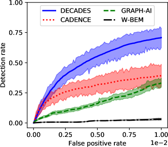
Figure 3. Truncated ROC curves of the 4 evaluated methods on the authentication events, with 95% confidence intervals.

We now present our experimental study of Decades, addressing three main questions: first, what does the model actually learn about the dataset? Secondly, does Decades perform well at detecting malicious behavior? Finally, to what extent do hyperparameters affect detection performance?

As for the first question, Figure 2 displays the weights $w^{e}_{ij}$ obtained after training. One rather unexpected outcome is that the destination of a remote authentication is mostly predicted through its type, while little importance is given to the user and source. One possible explanation is that the authentication type is correlated with the functional role of the destination host: for instance, most servers should be authenticated to using Kerberos, but some of them might only support NTLM. Similarly, remote desktop sessions might be primarily used by help desk employees to connect to malfunctioning workstations, while servers might be administered using different tools.

Table 4. Mean and 95% confidence interval of each evaluation metric. AUC@1% is the normalized area under the truncated ROC curve, and DR-$B$ is the proportion of red team events detected by extracting the $B$ most anomalous events each day. The best mean score for each metric is marked in bold.

Method	AUC@1%	DR-1K	DR-5K	DR-10K	DR-20K
Decades	0.497$\pm$0.085	0.081$\pm$0.032	0.333$\pm$0.060	0.482$\pm$0.076	0.640$\pm$0.099
Cadence	0.291$\pm$0.063	0.093$\pm$0.034	0.218$\pm$0.051	0.276$\pm$0.062	0.344$\pm$0.086
GraphAI	0.170$\pm$0.019	0.032$\pm$0.010	0.084$\pm$0.014	0.116$\pm$0.013	0.218$\pm$0.030
W-BEM	0.016$\pm$0.002	0.004$\pm$0.002	0.009$\pm$0.003	0.016$\pm$0.002	0.025$\pm$0.005

(a) Number of negative samples $K$

(b) Latent space dimension $d$

(c) Regularization coefficient $\lambda_{0}$

(d) Regularization coefficient $\lambda_{1}$

Figure 4. Area under the truncated ROC curve with 95% confidence intervals for several values of the hyperparameters.

In order to answer the second question, we compare Decades with three previously published methods: Cadence (Amin et al., 2019) and the language model of (Tuor et al., 2018) (referred to as W-BEM) are closest to our approach, making them the most relevant references. In particular, they both aim to fully address the combinatorics of events, not restricting themselves to pairwise interactions or entity-centric modelling. However, they focus only on authentications, whereas jointly modelling several event types is a key feature of our approach. We also include the graph-based model of (Bowman et al., 2020) (referred to as GraphAI), which differs by only modelling pairwise user-user and user-host interactions. Note that sec2graph (Leichtnam et al., 2020) and the pattern-based approach of (Siadati and Memon, 2017) would have been interesting baselines, but they both rely on explicit attributes of the entities, which are not available in the LANL dataset. The open-source implementation of W-BEM was used for the experiments. We reimplemented GraphAI based on (Bowman et al., 2020) and further precisions obtained from the authors. Finally, Cadence was implemented based only on (Amin et al., 2019) since the authors did not respond to our requests for code. As for hyperparameters, we reused those provided in the corresponding papers, except when different values gave better results.

Since all considered algorithms give non-deterministic results (mostly because of random parameter initialization and stochastic optimization procedures), each of them is run 20 times. We then report the mean and 95% confidence interval (obtained through a nonparametric bootstrap procedure) for each metric. Results are displayed in Table 4 and Figure 3. Decades globally outperforms competing algorithms, with significantly higher scores for all but one performance metric, namely the detection rate for a daily investigation budget of 1 000 events. Note that these scores remain rather low: for instance, investigating 10 000 events each day is a considerable amount of work, and it only leads to a 48% detection rate using Decades. However, it should be kept in mind that our aim is only to sort events so that the most suspicious ones rank close to the top, and further processing steps should then be applied to obtain more exploitable results (see Section 6 for more details).

As for competing methods’ performance, the best contender is Cadence. This confirms that Cadence’s approach to modelling the combinatorics of events, which Decades also relies upon, is indeed the most effective one. Next up is GraphAI, which only models dyadic interactions instead of fully leveraging the combinatorics of events. This simplified description of events can thus be considered too crude, once again backing up our hypothesis regarding the importance of factoring in the complexity of the data. Finally, W-BEM performs surprisingly poorly, which can be attributed to the inadequate data specification it relies upon. Indeed, the idea behind W-BEM is to treat events as sentences, with each involved entity representing a word. However, this representation ignores the specific structure of event logs: the number of involved entities as well as their types are fixed for all events of a given type, making the actual sample space much smaller than the set of all sequences of entities. In other words, W-BEM gives strictly positive probability to many samples which are actually not events and can thus never happen. This can be expected to make the model less efficient at learning to predict actual events. From a more general perspective, our experiments sustain our initial claim: carefully adapting the statistical model to the nature of the data leads to a better intrusion detection system.

We finally address the third question – namely, how sensitive is Decades’s detection performance to the value of each hyperparameter? To that end, we study the evolution of the area under the truncated ROC curve as one hyperparameter varies while the others are kept fixed to their optimal values. The results are displayed in Figure 4. The most striking observation is that the regularization coefficients $\lambda_{0}$ and $\lambda_{1}$ have no significant influence, suggesting that retraining makes little difference in our experiments. This is somewhat understandable given the short duration of the test phase, and it thus does not refute the importance of model updating in a real network monitoring setting. As for the other hyperparameters, the latent space dimension $d$ essentially controls the number of parameters of the model. As a consequence, it should be tuned so as to avoid both underfitting and overfitting. These two unwanted configurations can be observed in Figure 4(b), with the lowest value of $d$ yielding significantly inferior results and the highest one leading to increased uncertainty. Finally, the number of negative samples $K$ relates to the trade-off between the quality of the approximation of the log-likelihood gradient provided by NCE and the computational cost of training. Figure 4(a) shows that increasing $K$ beyond 10 does not make the model better at detecting malicious events. Note that detection performance even tends to decrease for high values of $K$, which may result from a kind of overfitting: as $K$ increases, the model more accurately fits the distribution of the training data. This might lead it to assign higher anomaly scores to rare but benign events, in turn yielding more false positives.

6. Discussion and Future Work

We now discuss some limitations and possible future improvements of our method. First of all, being an event log-based anomaly detection algorithm, Decades obviously has some common flaws: it relies on the integrity of the data, which means that advanced intruders could evade detection by tampering with the logs, and it actually detects unusual rather than malicious behavior. While the former is entirely out of the scope of this work, the latter can lead to interesting developments. In particular, the resilience of Decades to deliberate poisoning of the training set could be studied.

The most important improvement that could be brought to our approach is an interface making the alerts more exploitable. Two main directions could be explored. The first one is the interpretation of each anomalous event, which could rely on counterfactual explanations: given the entities involved in an anomalous event, which replacements would make the event normal? For instance, given the user, type and source host of an anomalous remote authentication, which possible destinations would be considered normal? The other way to make the results more usable is alert aggregation and correlation. Indeed, Decades reduces the workload of security experts by ranking events in descending order of anomalousness, allowing the expert to focus on the most anomalous events first. However, the number of events to review daily remains significant and needs to be further reduced, which could be done by merging events resulting from the same high-level activity. This issue has been widely addressed in the field of intrusion detection system alert postprocessing (Valdes and Skinner, 2001; Julisch, 2003; Roundy et al., 2017; Haas and Fischer, 2018; Lin et al., 2018).

Finally, improving the updating procedure of the model could be a more theoretical research direction. In particular, the procedure exposed here does not take into account the uncertainty associated with the estimated parameters. This can be problematic when operating on a long time range: by forgetting every day how confident the model was about each parameter, we might propagate errors due to unreliable estimates. A fully Bayesian approach, similar to the one proposed by (Lee et al., 2019) for host communication graphs, could solve this issue.

7. Conclusion

We propose Decades, a novel anomaly detection algorithm for event log data. This algorithm extends previous work in order to simultaneously address the three main challenges associated with event logs: combinatorial observations, heterogeneity and temporal concept drift. Our experiments show that handling the full complexity of event log data through a bespoke statistical model yields better detection results than the converse approach, namely simplifying the data enough to make them fit into more traditional anomaly detection frameworks. Therefore, we argue that this research direction should be explored further in order to build effective and robust intrusion detection systems for event logs.

One of the strengths of Decades is its adaptability: by making few assumptions about the content of the modelled events, we aim to make our algorithm independent of the chosen logging system. It would thus be interesting to extend the empirical study to other datasets, including for instance network logs. Our method could also be further improved through better alert interpretability and correlation, as well as uncertainty-aware parameter updates. With such additional features, the proposed model could evolve into a generic and reliable intrusion detection algorithm for various kinds of log data.

References

- (1)
- Adilova et al. (2019) Linara Adilova, Livin Natious, Siming Chen, Olivier Thonnard, and Michael Kamp. 2019. System Misuse Detection via Informed Behavior Clustering and Modeling. In DSN-W.
- Amin et al. (2019) Mohammad Ruhul Amin, Pranav Garg, and Baris Coskun. 2019. CADENCE: Conditional Anomaly Detection for Events Using Noise-Contrastive Estimation. In AISec.
- Bohara et al. (2017) Atul Bohara, Mohammad A Noureddine, Ahmed Fawaz, and William H Sanders. 2017. An Unsupervised Multi-Detector Approach for Identifying Malicious Lateral Movement. In SRDS.
- Bowman et al. (2020) Benjamin Bowman, Craig Laprade, Yuede Ji, and H Howie Huang. 2020. Detecting Lateral Movement in Enterprise Computer Networks with Unsupervised Graph AI. In RAID.
- Caruana (1997) Rich Caruana. 1997. Multitask learning. Mach. Learn. 28, 1 (1997), 41–75.
- Eldardiry et al. (2013) Hoda Eldardiry, Evgeniy Bart, Juan Liu, John Hanley, Bob Price, and Oliver Brdiczka. 2013. Multi-domain information fusion for insider threat detection. In S&P Workshops.
- Gonçalves et al. (2015) Daniel Gonçalves, João Bota, and Miguel Correia. 2015. Big data analytics for detecting host misbehavior in large logs. In Trustcom/BigDataSE/ISPA.
- Gutflaish et al. (2019) Eyal Gutflaish, Aryeh Kontorovich, Sivan Sabato, Ofer Biller, and Oded Sofer. 2019. Temporal anomaly detection: calibrating the surprise. In AAAI.
- Gutmann and Hyvärinen (2010) Michael Gutmann and Aapo Hyvärinen. 2010. Noise-contrastive estimation: A new estimation principle for unnormalized statistical models. In AISTATS.
- Haas and Fischer (2018) Steffen Haas and Mathias Fischer. 2018. GAC: graph-based alert correlation for the detection of distributed multi-step attacks. In SAC.
- Hu et al. (2017) Qiaona Hu, Baoming Tang, and Derek Lin. 2017. Anomalous User Activity Detection in Enterprise Multi-source Logs. In ICDM Workshops.
- Julisch (2003) Klaus Julisch. 2003. Clustering intrusion detection alarms to support root cause analysis. TISSEC 6, 4 (2003), 443–471.
- Kendall et al. (2018) Alex Kendall, Yarin Gal, and Roberto Cipolla. 2018. Multi-task learning using uncertainty to weigh losses for scene geometry and semantics. In CVPR.
- Kent (2015a) Alexander D. Kent. 2015a. Comprehensive, Multi-Source Cyber-Security Events. Los Alamos National Laboratory. https://doi.org/10.17021/1179829
- Kent (2015b) Alexander D. Kent. 2015b. Cybersecurity Data Sources for Dynamic Network Research. In Dynamic Networks in Cybersecurity. Imperial College Press.
- Kent et al. (2015) Alexander D Kent, Lorie M Liebrock, and Joshua C Neil. 2015. Authentication graphs: Analyzing user behavior within an enterprise network. Comput. Secur. 48 (2015), 150–166.
- Kingma and Ba (2014) Diederik P Kingma and Jimmy Ba. 2014. Adam: A method for stochastic optimization. arXiv preprint arXiv:1412.6980 (2014).
- Lee et al. (2019) Wesley Lee, Tyler H McCormick, Joshua Neil, and Cole Sodja. 2019. Anomaly detection in large scale networks with latent space models. arXiv preprint arXiv:1911.05522 (2019).
- Legg et al. (2015) Philip A Legg, Oliver Buckley, Michael Goldsmith, and Sadie Creese. 2015. Automated insider threat detection system using user and role-based profile assessment. IEEE Syst. J. 11, 2 (2015), 503–512.
- Leichtnam et al. (2020) Laetitia Leichtnam, Eric Totel, Nicolas Prigent, and Ludovic Mé. 2020. Sec2graph: Network Attack Detection Based on Novelty Detection on Graph Structured Data. In DIMVA.
- Lin et al. (2018) Ying Lin, Zhengzhang Chen, Cheng Cao, Lu-An Tang, Kai Zhang, Wei Cheng, and Zhichun Li. 2018. Collaborative alert ranking for anomaly detection. In CIKM.
- Liu et al. (2019) Fucheng Liu, Yu Wen, Dongxue Zhang, Xihe Jiang, Xinyu Xing, and Dan Meng. 2019. Log2vec: A Heterogeneous Graph Embedding Based Approach for Detecting Cyber Threats within Enterprise. In CCS.
- Mikolov et al. (2013) Tomas Mikolov, Ilya Sutskever, Kai Chen, Greg Corrado, and Jeffrey Dean. 2013. Distributed representations of words and phrases and their compositionality. In NeurIPS.
- Mnih and Kavukcuoglu (2013) Andriy Mnih and Koray Kavukcuoglu. 2013. Learning word embeddings efficiently with noise-contrastive estimation. NeurIPS (2013).
- Mnih and Teh (2012) Andriy Mnih and Yee Whye Teh. 2012. A fast and simple algorithm for training neural probabilistic language models. In ICML.
- Passino et al. (2020) Francesco Sanna Passino, Melissa JM Turcotte, and Nicholas A Heard. 2020. Graph link prediction in computer networks using Poisson matrix factorisation. arXiv preprint arXiv:2001.09456 (2020).
- Paszke et al. (2019) Adam Paszke, Sam Gross, Francisco Massa, Adam Lerer, James Bradbury, Gregory Chanan, Trevor Killeen, Zeming Lin, Natalia Gimelshein, Luca Antiga, et al. 2019. PyTorch: An Imperative Style, High-Performance Deep Learning Library.. In NeurIPS.
- Powell (2020) Brian A Powell. 2020. Detecting malicious logins as graph anomalies. J. Inf. Secur. Appl. 54 (2020), 102557.
- Rashid et al. (2016) Tabish Rashid, Ioannis Agrafiotis, and Jason RC Nurse. 2016. A new take on detecting insider threats: exploring the use of hidden markov models. In MIST.
- Roundy et al. (2017) Kevin A Roundy, Acar Tamersoy, Michael Spertus, Michael Hart, Daniel Kats, Matteo Dell’Amico, and Robert Scott. 2017. Smoke detector: cross-product intrusion detection with weak indicators. In ACSAC.
- Ruder (2017) Sebastian Ruder. 2017. An overview of multi-task learning in deep neural networks. arXiv preprint arXiv:1706.05098 (2017).
- Sexton et al. (2015) Joseph Sexton, Curtis Storlie, and Joshua Neil. 2015. Attack chain detection. Stat. Anal. Data Min. 8, 5-6 (2015), 353–363.
- Shashanka et al. (2016) Madhu Shashanka, Min-Yi Shen, and Jisheng Wang. 2016. User and entity behavior analytics for enterprise security. In BigData.
- Siadati and Memon (2017) Hossein Siadati and Nasir Memon. 2017. Detecting structurally anomalous logins within enterprise networks. In CCS.
- Siddiqui et al. (2019) Md Amran Siddiqui, Jack W Stokes, Christian Seifert, Evan Argyle, Robert McCann, Joshua Neil, and Justin Carroll. 2019. Detecting cyber attacks using anomaly detection with explanations and expert feedback. In ICASSP.
- Tang et al. (2017) Baoming Tang, Qiaona Hu, and Derek Lin. 2017. Reducing False Positives of User-to-Entity First-Access Alerts for User Behavior Analytics. In ICDM Workshops.
- Tuor et al. (2017) Aaron Tuor, Samuel Kaplan, Brian Hutchinson, Nicole Nichols, and Sean Robinson. 2017. Deep learning for unsupervised insider threat detection in structured cybersecurity data streams. In AAAI Workshops.
- Tuor et al. (2018) Aaron Randall Tuor, Ryan Baerwolf, Nicolas Knowles, Brian Hutchinson, Nicole Nichols, and Robert Jasper. 2018. Recurrent Neural Network Language Models for Open Vocabulary Event-Level Cyber Anomaly Detection. In AAAI Workshops.
- Turcotte et al. (2016b) Melissa Turcotte, Juston Moore, Nick Heard, and Aaron McPhall. 2016b. Poisson factorization for peer-based anomaly detection. In ISI.
- Turcotte et al. (2016a) Melissa JM Turcotte, Nicholas A Heard, and Alexander D Kent. 2016a. Modelling user behaviour in a network using computer event logs. In Dynamic Networks and Cyber-Security. World Scientific, 67–87.
- Valdes and Skinner (2001) Alfonso Valdes and Keith Skinner. 2001. Probabilistic alert correlation. In RAID.
- Veeramachaneni et al. (2016) Kalyan Veeramachaneni, Ignacio Arnaldo, Vamsi Korrapati, Constantinos Bassias, and Ke Li. 2016. : training a big data machine to defend. In BigDataSecurity.
- Yen et al. (2013) Ting-Fang Yen, Alina Oprea, Kaan Onarlioglu, Todd Leetham, William Robertson, Ari Juels, and Engin Kirda. 2013. Beehive: Large-scale log analysis for detecting suspicious activity in enterprise networks. In ACSAC.