Engineering Nearly Linear-Time Algorithms for Small Vertex Connectivity

Abstract

Vertex connectivity is a well-studied concept in graph theory with numerous applications. A graph is $k$-connected if it remains connected after removing any $k-1$ vertices. The vertex connectivity of a graph is the maximum $k$ such that the graph is $k$-connected. There is a long history of algorithmic development for efficiently computing vertex connectivity. Recently, two near linear-time algorithms for small $k$ were introduced by [Forster et al. SODA 2020]. Prior to that, the best known algorithm was one by [Henzinger et al. FOCS’96] with quadratic running time when $k$ is small.

In this paper, we study the practical performance of the algorithms by Forster et al. In addition, we introduce a new heuristic on a key subroutine called local cut detection, which we call degree counting. We prove that the new heuristic improves space-efficiency (which can be good for caching purposes) and allows the subroutine to terminate earlier. According to experimental results on random graphs with planted vertex cuts, random hyperbolic graphs, and real world graphs with vertex connectivity between 4 and 15, the degree counting heuristic offers a factor of 2-4 speedup over the original non-degree counting version for most of our data. It also outperforms the previous state-of-the-art algorithm by Henzinger et al. even on relatively small graphs.

1 Introduction

Given an undirected graph, the vertex connectivity problem is to compute the minimum size of a vertex set $S$ such that after removing $S$, the remaining graph is disconnected or a singleton. Such a vertex-set is called a minimum vertex cut. Vertex connectivity is well-studied concept in graph theory with applications in many fields. For example, for network reliability [13, 20], a minimum vertex-cut has the highest chance to disconnect the network assuming each node fails independently with the same probability; in sociology, vertex connectivity of a social network measures social cohesion [29].

There is a long history of algorithmic development for efficiently computing vertex connectivity (see [23] for more elaborated discussion of algorithmic development). Let $n$ and $m$ be the number of vertices and edges respectively in the input graph. The time complexity for computing vertex connectivity has been $O(n^{2})$ since 1970 [17] even for the special case where the connectivity is a constant until very recently, when [9] introduced randomized (Monte Carlo) algorithms to compute vertex connectivity in time $O(m+n\kappa^{3}\log^{2}n)$ (for undirected graphs) where $\kappa$ is the vertex connectivity of the graph. The algorithm follows the framework by [23]. This makes progress toward the conjecture (when $\kappa$ is a constant) by Aho, Hopcroft and Ullman [1] (Problem 5.30) that there exists a linear time algorithm for computing vertex connectivity. Before that, the state-of-the-art algorithm was due to [15], which runs in time $O(n^{2}\kappa\log n)$.

In this paper, we study the practical performance of the near-linear time algorithms by [9] for small vertex connectivity. We briefly describe their framework and point out the potential improvement of the framework. [23] provide a fast reduction from vertex connectivity to a subroutine called local vertex-cut detection. Roughly speaking, the framework deals with two extreme cases: detecting balanced cuts and unbalanced cuts. The balanced cuts can be detected using (multiple calls to) a standard $st$-max flow algorithm; the unbalanced cuts can be detected using (multiple calls to) local vertex-cut detection. Reference [9] follow the same framework and observe that local vertex-cut detection can be further reduced to another subroutine called local edge-cut detection as well as provide fast edge cut detection algorithms that finally prove the near-linear time vertex connectivity algorithm for any constant $\kappa$. The full algorithm is discussed in Appendix B. From our internal testing, we observe that, overall the framework, the performance bottleneck is on the local edge detection algorithm.

Therefore, our focus is on speeding up the local edge-cut detection algorithm. To define the problem precisely, we first set up notations. Let $G=(V,E)$ be a directed graph. Let $E(S,T)$ be the set of edges from vertex-set $S$ to vertex-set $T$. For any vertex-set $S$, let $\operatorname{vol}^{\operatorname{out}}(S):=\sum_{v\in S}\operatorname{deg}^{\operatorname{out}}(v)$ denote the volume of $S$ which is total number of edges originating in $S$. Undirected edges are treated as one directed edge in each direction. We now define the interface of the local edge-cut detection algorithm.

Definition 1.1.

An algorithm $\mathcal{A}$ is LocalEC if it takes as input a vertex $x$ of a graph $G=(V,E)$, and two parameters $\nu,k$ such that $\nu k=O(|E|)$, and output in the following manner:

• either output a vertex-set $S$ such that $x\in S$ and $|E(S,V\setminus S)|<k$ or,

• the symbol $\bot$ certifying that there is no non-empty vertex-set $S$ such that

  $$x\in S,\operatorname{vol}^{\operatorname{out}}(S)\leq\nu,\mbox{ and }|E(S,V\setminus S)|<k.$$ (1)

The algorithm is allowed to have bounded one-sided error in the following sense. If there is a non-empty vertex-set $S$ satisfying Equation 1 then $\bot$ is returned with probability at most $1/2$.

Reference [9] introduced two LocalEC algorithms with the running time $O(\nu k^{2})$. The algorithms are very simple: they use repeated DFS (depth-first search) with different conditions for early termination. We note that this running time is enough to get a near-linear time algorithm for small connectivity using the framework by [23].

Our Results and Contribution. We introduce a heuristic called degree counting that is applicable to both variants of LocalEC in [9], which we call Local1+ and Local2+. We prove that the degree counting heuristic version is more space-efficient in terms of edge-query complexity and vertex-query complexity. Edge-query complexity is defined as the number of edges that the algorithm accesses, and vertex-query complexity is defined as the number of vertices that the algorithm accesses. The results are shown in Table 1. These complexity measures can be relevant in practice. For example, an algorithm with low query complexity may be able to store the accessed data in a smaller cache than an algorithm with high query complexity.

Table 1: Comparisons among various implementation of LocalEC algorithms. Local1+ denotes Local1 with the degree counting heuristic. Similarly, Local2+ denotes Local2 with the degree counting heuristic.

LocalEC Variants	Time	Edge-query	Vertex-query	Reference
Local1	$O(\nu k^{2})$	$O(\nu k^{2})$	$O(\nu k^{2})$	[9]
Local1+	$O(\nu k^{2})$	$O(\nu k^{2})$	$O(\nu k)$	This paper
Local2	$O(\nu k^{2})$	$O(\nu k)$	$O(\nu k)$	[9]
Local2+	$O(\nu k^{2})$	$O(\nu k)$	$O(\nu)$	This paper

We conducted experiments on three types of undirected graphs: (1) graphs with planted cuts where we have control over size and volume of the cuts, and (2) random hyperbolic graphs, and (3) real-world networks. We denote LOCAL1, LOCAL1+, and LOCAL2+ to be the same local-search based vertex connectivity algorithm [9] (see Appendix B for details) except that the unbalanced part is implemented with different LocalEC algorithms using Local1, Local1+, Local2+, respectively. We use Local1 as a baseline for LocalEC algorithms. We denote HRG to be the preflow-push-relabel-based algorithm by [15]. We implement HRG as a baseline because when $k$ is small (say $k=O(1)$) HRG is the fastest known alternative to [9, 23]. The implementation detail can be found in Appendix C. By sparsification algorithm [22], we can assume that the input graph size depends on $n$ and $k$. The following summarize the key finding of our empirical studies.

1. Internal Comparisons (Section 5.5). We compare three LocalEC algorithms (Local1, Local1+, Local2+). According to the experiments (Figure 6), for any $\nu$ parameter, Local1+ and Local2+ visit significantly fewer edges than Local1. Also, Local2+ visits slightly fewer edges than Local1+ overall. The degree counting is also very effective at low volume parameter. When plugging into full vertex connectivity algorithms, the degree counting heuristics (LOCAL1+ and LOCAL2+) improve the performance over non-degree counting counter part (LOCAL1) by a factor 2 to 4 for most data used in our experiments, although for some larger graphs the speedup was noticeably larger. The greatest observed speedup over LOCAL1 is 18.4x for LOCAL2+ at $n=100000$, $\kappa_{G}=16$. For graphs of this size, LOCAL2+ performs slightly better than LOCAL1+. Finally, according to CPU sampling, the local search is the main bottleneck for the performance of LOCAL1 at roughly at least $90\%$ for large instances. On the other hand, for the degree counting versions (LOCAL1+ and LOCAL2+), the CPU usage of local search part is improved to be almost the same as the other main component (i.e., finding a balanced cut using the Ford-Fulkerson’s max-flow algorithm).

2. Comparisons to HRG. We compare four vertex connectivity algorithms, namely HRG, LOCAL1, LOCAL1+, LOCAL2+. For planted cuts (Section 5.2), LOCAL1, LOCAL1+, and LOCAL2+ scale with $n$ much better than HRG when $\kappa_{G}$ is fixed. In particular, LOCAL1+ and LOCAL2+ start to outperform HRG on graphs as small as $n\leq 500$ (when $\kappa\leq 15$). For random hyperbolic graphs (Section 5.3), HRG performs much better than on the planted cut instances, but is still outperformed relatively early. In particular, LOCAL1+ and LOCAL2+ outperform HRG for $n\geq 5000$ when $\kappa\leq 12.$ In real-world graphs (Section 5.4), LOCAL1+ and LOCAL2+ are the fastest among the four algorithms with LOCAL2+ being slightly faster than LOCAL1+. We also observe that the performance of all four algorithms is very similar on part of the real world dataset and graphs with planted cuts with the same size and vertex connectivity.

Organization. We discuss related work in Section 2, and preliminaries in Section 3. Then, we review two variants of LocalEC algorithms (Local1,Local2) [9], and describe new degree counting heuristic versions (Local1+, Local2+) in Section 4. Then, all the experimental results are discussed in Section 5. We conclude and discuss future work in Section 6.

2 Related Work

Fast Vertex Connectivity Algorithms. We consider a decision version where the problem is to decide if $G$ has a vertex cut of size at most $k-1$ (the general vertex connectivity can be solved using a binary search on $k$). We highlight only recent state-of-the-art algorithms. For more elaborated discussion, see [23]. When $k=O(1)$, the fastest known algorithm is by [9] with running time $O(m+nk^{3}\log^{2}n)$. The algorithm is based on local search approach. For larger $k$, the fastest known algorithm are based on preflow-push-relabel by [15] with the running time $O(n^{2}k\log n)$, and based on algebraic techniques by [19] with the running time $O(n^{\omega}\log^{2}n+k^{\omega}n\log n)$ where $\omega$ denotes the matrix multiplication exponent, currently $\omega\leq 2.37286$ [2]. When $k$ is small (say $k=O(1)$), the preflow-push-relabel-based algorithm by [15] is the fastest alternative to [9, 23]. Therefore, we implement the preflow-push-relabel-based algorithm [15] as a baseline for performance comparisons. We note both all aforementioned algorithms are randomized. Deterministic algorithms are much slower than the randomized ones. The fastest known deterministic algorithms are by [10] for large $k$ and by [11] for $k=O(1)$.

Deciding $(k,s,t)$-Vertex Connectivity. We mention another related problem which is to decide if the there is a vertex cut separating $s$ and $t$ of size at most $k-1$. By a standard reduction [7], it can be solved by $st$-maximum flow. $st$-maximum flow can be solved in time $O(mk)$ by augmenting paths algorithm by Ford-Fulkerson algorithm [8]. For larger $k$, a simple blocking flow algorithm by [6] runs in time $O(m\sqrt{n})$. The current state-of-the art algorithms are $O(m^{4/3+o(1)})$-time algorithm by [21], and $\tilde{O}(m+n^{1.5})$-time algorithm by [27]. Note that when $k$ is small (e.g., $k=O(1)$), then Ford-Fulkerson algorithm [8] is the fastest, and we thus implement Ford-Fulkerson algorithm as a subroutine to find vertex cut for the balanced case.

Local Search. There are quite a few local search algorithm with different running time. The first LocalEC algorithm by [4] has running time of $O(\nu k^{k})$. [9] introduced a new local search algorithm with improved time $O(\nu k^{2})$. [9] also provide a reduction to local vertex cut detection problem, which we called LocalVC (similar to Definition 1.1, but uses vertex cut instead of edge cut). Therefore, there is a LocalVC algorithm with running time $O(\nu k^{2})$. This improved the previous bound for LocalVC with running time $O(\nu^{1.5}k)$ by [23] when $k$ is small. For our purpose, when $k$ is small (say $k=O(1)$), the algorithm by [9] is the fastest, and thus we consider the LocalEC algorithm by [9].

Implementation and Experimental Studies. To the best of our knowledge, this paper is the first experimental study on vertex connectivity algorithms; there were no prior experimental studies on vertex connectivity algorithms. This is in stark contrast to the edge-connectivity problem (which is considered as a sibling problem) where we compute the minimum number of edges to be removed to disconnect the graph. For edge-connectivity, there are many experimental studies [16, 5, 24, 14]. More recently, the work by [12] implemented the local search framework in [9] to compute directed edge-connectivity.

3 Preliminaries

Let $G=(V,E)$ be an undirected graph. In general, we denote $m=|E|$ and $n=|V|$. We denote $E(S,T)$ be the set of edges from vertex-set $S$ to vertex-set $T$. We say that $S\subset V$ is a vertex cut if $G-S$ (the graph after removing $S$ from $G$) is disconnected. If no vertex cut of size $k$ exists, the graph is k-(vertex)-connected. We say that $S$ is an $xy$-vertex cut if $x$ cannot reach $y$ in $G-S$. Let $\kappa_{G}$ be vertex connectivity of $G$, i.e., the size of the minimum vertex-cut (or $n-1$ if no cut exists). Let $\kappa_{G}(x,y)$ denote the size of the minimum $xy$-vertex cut in $G$ or $n-1$ if the $xy$-vertex cut does not exist. We say that a triplet $(L,S,R)$ is a separation triple if $L,S$ and $R$ form a partition of $V$, $L$ and $R$ are not $\emptyset$ and $E(L,R)=\emptyset$. In this case, $S$ is a vertex-cut in $G$. The decision problem for vertex connectivity which we call $k$-connectivity problem is the following: Given $G=(V,E)$, and integer $k$, decide if $G$ is $k$-connected, and if not, output a vertex-cut of size $<k$.

Sparsification. For an undirected graph $G=(V,E)$, the algorithm by Nagamochi and Ibaraki [22] runs in $O(m)$ time and partitions $E$ into a sequence of forests $E_{1},\ldots,E_{n}$ (possibly $E_{i}=E_{i+1}=\ldots=E_{n}=\emptyset$ for some $i$). For each $k\leq n$, the subgraph $FG_{k}:=(V,\bigcup_{i\leq k}E_{i})$ has the property that $FG_{k}$ is $k$-connected if and only if $G$ is $k$-connected. Moreover, any vertex cut of size $<k$ in $FG_{k}$ is also a vertex cut in $G$. Clearly, $|E(FG_{k})|\leq nk$.

From now, with preprocessing in $O(m)$ time, we assume that the input graph to the $k$-connectivity problem is $FG_{k}$. In particular, we can assume that the number of edges is $O(nk)$. We can also assume that the minimum degree is at least $k$ (because otherwise we can output the neighbor of the vertex with minimum degree).

Split Graph. The split graph construct is a standard reduction from vertex connectivity based problems to edge connectivity based problems, used in the algorithms featured in this paper, among others [7, 9, 15]. Given graph $G$, we define the split graph $SG$ as follows. For each vertex $v$ in $G$, we replace $v$ with an “in-vertex” $v_{\operatorname{in}}$ and an “out-vertex” $v_{\operatorname{out}}$, and add an edge from $v_{\operatorname{in}}$ and $v_{\operatorname{out}}$. The reduction follows from the observation that edge-disjoint paths in $SG$ that start at an outvertex and end at an invertex correspond to (non-endpoint) vertex-disjoint paths in $G$. For each edge $(u,v)$ in $G$, we add an edge from $(v_{\operatorname{in}},u_{\operatorname{out}})$ in $SG$.

4 LocalEC Algorithms and Degree Counting Heuristics

In this section, we review two variants of LocalEC algorithms by [9], and describe their corresponding new version using the degree counting heuristic. For completeness, we describe the complete vertex connectivity algorithm by [9] and some implementation details in Appendix B. All the algorithms in this section follow a common framework called AbstractLocalEC as described in Algorithm 1. Let $G=(V,E)$ be the graph that we work on. The algorithm takes as inputs $x\in V$ and two integers $\nu,k$. The basic idea is to apply Depth-first Search (DFS) on the starting vertex $x$ but force early termination. We repeat for $k$ iterations. If DFS terminates normally at some iteration, i.e., without having to apply the early termination condition, then the set of reachable vertices satisfy Equation 1. Otherwise, we certify that no cut satisfying Equation 1 exists. The only main difference is at line 1 where we need to specify the condition for early termination and selection of the vertex $y\in V(T)$ in such a way that the entire algorithm outputs correctly with constant probability. If the minimum degree is less than $k$, we set $k$ to the minimum degree and return the trivial cut if no smaller cut is found.

• repeat for $k$ times:

  1. Grow a DFS tree $T$ starting from $x$, stopping early at some point to obtain $y\in V(T)$.

  2. If the DFS terminates normally, then return $V(T)$.

  3. Reverse all edges along the unique path from $x$ to $y$ in the tree $T$, unless this is the last iteration.

• return $\bot$.

Algorithm 1 AbstractLocalEC${}_{G}(x,\nu,k)$

Next, we define time and space complexity (in terms of edges and vertices required to run the algorithm) of a LocalEC algorithm.

Definition 4.1.

Let $\mathcal{A}(x,\nu,k)$ be a LocalEC algorithm. $\mathcal{A}$ has $(t,s_{e},s_{v})$-complexity if $\mathcal{A}$ terminates in $O(t)$ time and accesses at most $O(s_{e})$ distinct edges, and at most $O(s_{v})$ distinct vertices.

4.1 Local1 and Degree Counting Version

Algorithm for Local1. Replace line 1 in Algorithm 1 with the following process. Grow a DFS tree starting on vertex $x$ and stop when the number of accessed edges is exactly $8\nu k$. Let $E^{\prime}$ be the set of accessed edges. We sample an edge $(u,v)\in E^{\prime}$ uniformly at random. Finally, we set $y\leftarrow u$. If we sample $(u,v)$ to be the $\tau$-th edge visited, we can stop the DFS early after that edge (similarly to Local1+ below).

Theorem 4.2 (Theorem A.1 in [9]).

Local1$(x,\nu,k)$ is LocalEC with $(\nu k^{2},\nu k^{2},\nu k^{2})$-complexity.

Next, we present the degree counting version of Local1, which we call Local1+.

Algorithm for Local1+. Replace line 1 in LABEL:alg:abstractlocalec with the following process. Let $\tau$ be a random integer in the range $[1,8\nu k]$. If this is in the last iteration, we set $\tau\leftarrow 8\nu k$. Then, we grow a DFS tree $T$ starting on vertex $x$. At any time step, let $V(T)$ be the set of vertices visited by the DFS so far. We stop as soon as $\operatorname{vol}^{\operatorname{out}}(V(T))\geq\tau$. Finally, we set $y$ to be the last vertex that the DFS visited.

Theorem 4.3.

Local1+$(x,\nu,k)$ is LocalEC with $(\nu k^{2},\nu k^{2},\nu k)$-complexity.

4.2 Local2 and Degree Counting Version

We say that an edge is new if it has not been accessed in earlier iterations. Otherwise, it is old. It follows that reversed edges are old.

Algorithm for Local2. Replace line 1 in Algorithm 1 with the following process. We grow a DFS tree $T$ starting at vertex $x$. Let $E^{\prime}(T)$ be the set of new edges visited. We stop as soon as $E^{\prime}(T)\geq 8\nu$. Let $(u,v)$ be a random edge in $E^{\prime}(T)$. Finally, we set $y\leftarrow u$. We do not need to store $E^{\prime}(T)$ to sample from if we sample $\tau$ in the range $[1,8\nu]$ and choose the $\tau$-th new edge.

Theorem 4.4 (Equivalent to Theorem 3.1 in [9]).

Local2$(x,\nu,k)$ is LocalEC with $(\nu k^{2},\nu k,\nu k)$-complexity.

Next, we present the degree counting version of Local2, which we call Local2+. The algorithm is slightly more complicated. We set up notations. For each $v\in V$, let $c(v)$ be the remaining capacity for $v$, representing uncounted edge volume. Initially, $c(v)=\operatorname{deg}^{\operatorname{out}}(v)$.

Algorithm for Local2+. Replace line 1 in LABEL:alg:abstractlocalec with the following process. Let $\tau$ be a random integer in the range $[1,8\nu k]$. We grow a DFS tree starting on vertex $x$. At any time step, let $v_{1},v_{2},...,v_{i}$ be the sequence of vertices visited by the DFS so far. For the first vertex where $\sum_{j\leq i}c(v_{j})\geq\tau$, we set $y\leftarrow v_{i}$. As soon as $\sum_{j\leq i}c(v_{j})\geq 8\nu$, we stop the DFS and update the remaining capacity $c(v)$ on each $v$ as follows. We set $c(v_{j})\leftarrow 0$ for all $j<i$ and set $c(v_{i})\leftarrow\sum_{j\leq i}c(v_{j})-8\nu$.

Intuitively, we collect previously uncounted outgoing edges and choose the origin vertex for one of them at random.

Theorem 4.5.

Local2+$(x,\nu,k)$ is LocalEC with $(\nu k^{2},\nu k,\nu)$-complexity.

4.3 Proof of Theorems 4.2, 4.3, 4.4 and 4.5

In this section, we address proofs for Theorems 4.2, 4.3, 4.4 and 4.5.

Correctness. It can be shown that all four algorithms (Local1, Local1+, Local2, Local2+) are LocalEC through a similar argument as used in [9]. For completeness, we provide the proofs in Appendix A.

Complexity. Let $\mathcal{A}$ be an LocalEC algorithm (Definition 1.1), and let $\nu$, and $k$ be the parameters of the algorithm. We define three measure of complexity $T(\mathcal{A},G),U_{E}(\mathcal{A},G),$ and $U_{V}(\mathcal{A},G)$ on input graph $G$ and LocalEC algorithm $\mathcal{A}$ as follows. Let $T(\mathcal{A},G)$ be the number of times that the algorithm accesses edges on the input graph $G$. $T(\mathcal{A},G)$ measures time complexity of the algorithm. Let $U_{E}(\mathcal{A},G)$ be the number of unique edges accessed by the algorithm on graph $G$. This measures how much information (in terms of number of edges) that the algorithm needs to run. Let $U_{V}(\mathcal{A},G)$ be the number of unique vertices accessed by the algorithm on graph $G$.

For any graph $G$ and LocalEC algorithm $\mathcal{A}$, $T(\mathcal{A},G)\geq U_{E}(\mathcal{A},G)\geq U_{V}(\mathcal{A},G)$.

Local1. To see that Local1 has $(O(\nu k^{2}),O(\nu k^{2}),O(\nu k^{2}))$-complexity, it is enough to prove that $T(\text{Local1},G)=O(\nu k^{2})$. This follows easily because each iteration we stop the DFS after visiting exactly $8\nu k$ edges, and there are at most $k$ iterations.

Local1+. We first prove that $T(\text{Local1+},G)=O(\nu k^{2})$. Since there are $k$ iterations, it is enough to bound one iteration. Let $S$ be the set of vertices visited by the DFS before the step at which it stops early. Clearly, $\operatorname{vol}^{\operatorname{out}}(S)<8\nu k$, or we would have stopped earlier. By design, new edges can be only visited within the set $E(S,S)$ or at the last step. Therefore, the number of edges visited is at most $|E(S,S)|+1\leq\operatorname{vol}^{\operatorname{out}}(S)+1=O(\nu k)$ per iteration and $O(\nu k^{2})$ in total. We have $T(\text{Local1+},G)=O(\nu k^{2})$.

Remember that if the minimum degree is initially at least $k$ to avoid trivial cuts. When paths are reversed, no vertex other than $x$ will have reduced degree. Therefore we have $k(|S|-1)\leq\operatorname{vol}^{\operatorname{out}}(S)<8\nu k$. It follows that we visit at most $O(\nu)$ vertices in each iteration and $O(\nu k)$ in total.

Local2. We first prove that $U_{E}(\text{Local2},G)=O(\nu k)$. By design, for each iteration, we collect at most $8\nu$ new edges. Since we repeat for $k$ iterations, we collect at most $8\nu k$ total new edges. Next, we prove $T(\text{Local2},G)=O(\nu k^{2})$. Since each edge can be revisited at most $k$ times, we have $T(\text{Local2},G)\leq kU_{E}(\text{Local2},G)=O(\nu k^{2})$.

Local2+. We first prove that $U_{E}(\text{Local2+},G)=O(\nu k)$. If true, then we also have $T_{E}(\text{Local2+},G)\leq kU_{E}(\text{Local2+},G)=O(\nu k^{2})$. We will never visit an outgoing edge of vertex $v$ unless all its capacity has been exhausted. Therefore the total used capacity (at most $k$ times $8\nu$) is an upper bound for the number of distinct edges visited. For $U_{V}(\text{Local2+},G)$, fix any iteration. Let $S$ be the set of vertices visited by the DFS one step before terminating and $S^{\prime}\subseteq S$ the subset of $S$ that have not been visited before. Clearly, we have $k|S^{\prime}|\leq\operatorname{vol}^{\operatorname{out}}(S^{\prime})=\sum_{v\in S^{\prime}}c(v)\leq\sum_{v\in S}c(v)<8\nu$. The first inequality follows since the minimum degree is at least $k$. We visit at most $|S^{\prime}|+1=O(\nu/k)$ distinct vertices per iteration for a total of $O(\nu)$ distinct vertices.

5 Experimental Results

5.1 Experimental Setup

The algorithms were implemented and compiled using C++17 with Microsoft Visual Studio 2019. All experiments were run on a Windows 10 computer with Intel i7-9750H CPU (2.60GHz) and 16 GB DDR4-2667 RAM.

Four algorithms are compared. LOCAL1, LOCAL1+ and LOCAL2+ are implementations based on the algorithm by Forster et al [9]. The full algorithm to compute vertex connectivity using LocalEC is described in Appendix B and originally by [23]. LOCAL1 and LOCAL1+ use Local1 and Local1+ as their LocalEC algorithm with $2\nu k$ substituted for $8\nu k$. LOCAL2+ uses the LocalEC algorithm Local2+ with $3\nu$ substituted for $8\nu$. HRG is an implementation of the randomised version of the algorithm by Henzinger, Rao and Gabow [15]. The implementation details are described in Appendix C. All algorithms were implemented using parameters that bound theoretical success probability from below by a roughly equal constant. Since the data consists of undirected graphs only, the sparsification algorithm by Nagamochi and Ibaraki [22] is used together with each algorithm. The $O(m)$ partitioning of the edges into disjoint forests is not included in the measured time. Construction of the sparse graphs in $O(nk)$ time is included. As a result, none of the algorithms have time complexity dependent on m. Graph size is reported only in terms of vertices.

5.1.1 Data

The data consists of random graphs with planted vertex cuts, random hyperbolic graphs and real world data.

The first artificial dataset consists of graphs with a planted unique minimum vertex cut, which can be generated with full control over vertex connectivity and balancedness. We partition a complete graph into three sets $L$, $S$ and $R$ and use a subset of the edges in $E\setminus E(L,R)$, chosen using a modified version of the sparsification algorithm by Nagamochi and Ibaraki [22]. Like Nagamochi and Ibaraki, we label the edges to partition them into disjoint forests $\{E_{1},E_{2},...\}$ such that $(x,y)\in E_{i}$ implies that there is a path between $x$ and $y$ in $E_{1},E_{2},...,E_{i-1}$. Nagamochi and Ibaraki show that if this property holds for all edges, then the union of the $k$ first forests is $k$-connected if the original graph is $k$-connected. Unlike Nagamochi and Ibaraki, we randomly partition the edges by placing them in the applicable forest with the lowest index in a random order. We choose $k=60>|S|$ to guarantee that $S$ is a unique vertex cut that separates $L$ from $R$. For each set of parameters we generate five graphs and run the algorithm five times each and report the average.

The second artificial dataset consists of random hyperbolic graphs, generated using NetworKIT [26], which provides an implementation of the generator by von Looz et al. [28]. The properties of random hyperbolic graphs include a degree distribution that follows a power law and small diameter, which are common in real world graphs [3]. The graphs are generated with average degree 32 and a power law exponent of 10. We generate 20 graphs each for sizes $2^{10},2^{11},...,2^{18}$ vertices and group them according to vertex connectivity. We run the algorithm five times per graph and report the average for each group with the same size and vertex connectivity.

The real world data is based on three graphs from the SNAP dataset [18], soc-Epinions1, com-LiveJournal and web-BerkStan. The LiveJournal dataset is originally undirected. The other two are directed graphs read as undirected, which means that we compute weak vertex connecitivity for these graphs. We preprocess these graphs by taking the largest connected component for a $k$-core. A $k$-core is defined as the edge-maximal subgraph with minimum degree at least $k$. Only $k$-cores whose vertex connectivity is over 1 but less than the minimum degree are used. For each $k$-core we run the algorithms 25 times and report the average.

5.2 Planted Cuts

In theory the running time for HRG is linear in $\kappa$ and the algorithms based on Forster et al. [9] are cubic in $\kappa$. Figure 1(a) shows that the running time for HRG indeed grows much slower with $\kappa$. The running time for LOCAL1 exceeds that of HRG much earlier, at $\kappa\geq 17$, than LOCAL1+ ($\kappa\geq 40$) and LOCAL2+ ($\kappa\geq 48$).

Figure 1(b) shows that all four algorithms perform reasonably well both for graphs with unbalanced cuts and balanced cuts, although HRG is faster for unbalanced graphs by a factor of 2. Internal testing suggests that the running time of HRG is roughly proportional to $|L|^{2}+|R|^{2}$. The difference between the highest and lowest running time is a factor of 1.99 for HRG, 1.19 for LOCAL1, 1.27 for LOCAL1+ and 1.16 for LOCAL2+.

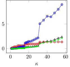
(a) $|L|=5$, $n=1000$

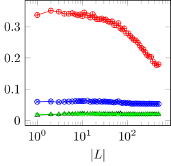
(b) $\kappa=5$, $n=1000$

(c) *

Figure 1: Running time (seconds) for Planted Cuts with variable $|L|$ or $\kappa$

When $\kappa<16$, LOCAL1, LOCAL1+ and LOCAL2+ outperform the quadratic-time HRG on very small graphs with planted cuts. At $\kappa=4$ in figure 2(a), HRG takes 23 ms for 100 vertices, which is already slower than both LOCAL1+ and LOCAL2+. LOCAL1 is faster than HRG at $n\geq 200$. When $\kappa=15$ (figure 2(d)), HRG is slower than LOCAL1+ and LOCAL2+ at $n\geq 250$ and LOCAL1 at $n\geq 550$.

LOCAL1+ and LOCAL2+ perform very similarly for small graphs but on larger graphs, LOCAL2+ is faster, as shown by figure 2(e).

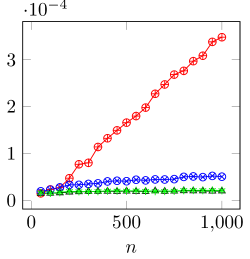
(a) $\kappa=4$, $|L|=5$

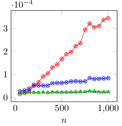
(b) $\kappa=7$, $|L|=5$

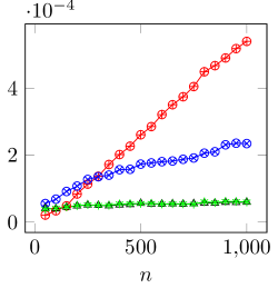
(c) $\kappa=8$, $|L|=5$

(d) $\kappa=15$, $|L|=5$

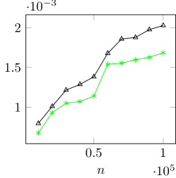
(e) $\kappa=31$, $|L|=5$

(f) *

Figure 2: Running time (seconds) per vertex for Planted cuts with fixed $|L|$ and $|S|$

5.3 Random Hyperbolic Graphs

HRG is much faster on random hyperbolic graphs than on the planted cut dataset. Comparing figures 2(c) and 3(c), the performance of HRG on 1000 vertex graphs with planted cuts of size 8 is similar to that on random hyperbolic graphs with the same vertex connectivity and over 30000 vertices. The performance differences are smaller for LOCAL1, LOCAL1+ and LOCAL2+, which means that the point at which these algorithms outperform HRG occurs at somewhat higher $n$.

For random hyperbolic graphs with $\kappa=7$ (figure 3(b)), HRG and LOCAL1 are equally fast at 4096 vertices (0.6 seconds). HRG is faster than LOCAL1 for all included random hyperbolic graphs where $\kappa>7$, including graphs up to 32768 vertices. The running time for LOCAL1+ and LOCAL2+ is close to that of HRG for random hyperbolic graphs where $\kappa=12$ and $n\in[1024,4196]$ (figure 3(e)).

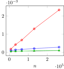
(a) $\kappa=4$

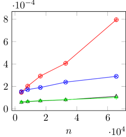
(b) $\kappa=7$

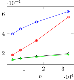
(c) $\kappa=8$

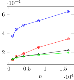
(d) $\kappa=10$

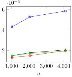
(e) $\kappa=12$

(f) *

Figure 3: Running time (seconds) per vertex for Random Hyperbolic Graphs

5.4 Real-World Networks

Figure 4 presents real world network data. Each row represents a $\delta$-core, where $\delta$ is the minimum degree of the resulting graph. Note that in general, minimum degree for a $k$-core can exceed $k$. Figure 5 shows data for graphs with planted cuts with similar parameters to the real world graphs, for comparison.

LOCAL1+ and LOCAL2+ clearly outperform LOCAL1 on real-world networks, as on artificial data. The $k$-cores of soc-Epinions1 have very similar performance in real world networks and graphs with planted cuts in figure 5. Performance for other real network data is generally faster for all four algorithms than for planted cuts, especially for HRG, which is 5-8 times faster on real world data. Similarly, running times for LOCAL1, LOCAL1+ and LOCAL2+ are also higher on random hyperbolic graphs than on $k$-cores of com-lj.ungraph and web-BerkStan.

Figure 4: Running times (milliseconds) per vertex on $k$-cores for real world networks

Figure 5: Running times (milliseconds) per vertex on Planted Cuts ($|L|=5$)

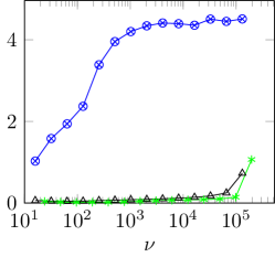
(a) k=8, $\frac{E_{LocalEC}}{\nu k}$

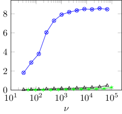
(b) k=16, $\frac{E_{LocalEC}}{\nu k}$

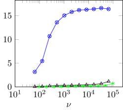
(c) k=32, $\frac{E_{LocalEC}}{\nu k}$

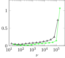
(d) k=8, $\frac{E_{LocalEC}}{\nu k}$

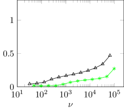
(e) k=16, $\frac{E_{LocalEC}}{\nu k}$

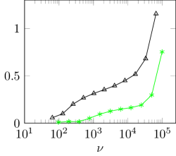
(f) k=32, $\frac{E_{LocalEC}}{\nu k}$

(g) *

Figure 6: Planted cuts with $n=100000,|L|=5,k=\kappa$
(Non-unique) average edges per LocalEC call, normalised by $\nu k$

5.5 Effectiveness of Degree Counting

In figure 6 we study internal measurements from LocalEC in the different algorithms. Note that Local1 and Local1+ apply a multiplicative factor of 2 to $\nu$ and Local2+ a factor of 3. The values used here include this increase. The number of edges visited by the average call to LocalEC at each value for $\nu$ is normalised by $\nu k$. This metric approximately doubles for Local1 and Local1+ when $k$ is doubled, as expected for algorithms quadratic in $k$. The metric grows for Local2+ too, but by a smaller factor around 1.5 for most values. The growth is faster for higher values for $\nu$ and for the highest values it is approximately by a factor 2, like the other two algorithms.

The number of edges explored relative to $\nu$ is higher for high $\nu$ for all algorithms and parameters in figure 6. For LOCAL1, it converges towards $\frac{\nu k}{2}$, which is the average of $[1,\nu k]$, the range of possible early stopping points $\tau$.

Local1 clearly visits more edges than in Local1+ and Local2+ by a large factor, according to figure 6. Figure 7 shows that most of the running time of LOCAL1 is used searching for unbalanced cuts with LocalEC. However, LOCAL1+ and LOCAL2+ spend a similar amount of time on balanced and unbalanced cuts. The only difference between the versions is the choice of LocalEC. These results suggest that degree counting improves the practical performance of LocalEC significantly but there is not much more room for improvement through LocalEC without also further optimising x-y max flow to search for balanced cuts. When the number of vertices is increased by a factor of 10, the time spent searching for unbalanced cuts does not seem to grow faster than the time spent searching for balanced cuts. The category “other” is dominated by initial setup for the data structures.

(a) $n=10000,\kappa=8$

(b) $n=10000,\kappa=16$

(c) $n=100000,\kappa=8$

(d) $n=100000,\kappa=16$

Figure 7: CPU use: balanced cuts/Ford-Fulkerson(FF) vs unbalanced cuts/LocalEC(Local).
Running time was measured separately.

5.6 Success rate

We define the success rate of a vertex connectivity algorithm as the percentage of attempts that yields an optimal cut. The observed success rate for HRG is at or near 100% on all featured datasets. For random hyperbolic graphs, none of the algorithms returned nonoptimal cuts. For graphs with planted cuts and $k$-cores of real world networks, the success rates are 97%+ for LOCAL1, 96%+ for LOCAL1+ and 95%+ for LOCAL2+.

6 Conclusion and Future Work

We study the experimental performance of the near-linear time algorithm by [9] when the input graph connectivity is small. The algorithm is based on local search. We also introduce a new heuristic for the local search algorithm, which we call degree counting. Based on experimental results, the degree counting heuristic significantly improves the empirical running time of the algorithm over its non-degree counting counterpart. For future work, we plan to extend the experiments to directed graphs, and on larger instances of datasets (order of millions edges).

Appendix A Omitted Proofs

A.1 Correctness

To show that any algorithm among Local1, Local1+, Local2, and Local2+ is LocalEC, it is enough to prove that it satisfies two properties:

If $V(T)$ is returned, then $|E(V(T),V-V(T))|<k$ and $\emptyset\neq V(T)\subsetneq V$.

If there is a vertex-set $S$ satisfying Equation 1, then $\bot$ is returned with probability at most $1/2$.

The following simple observation is due to [4]. Let $S$ be a vertex-set in graph $G$ and $x\in S$. Let $P$ be a path from $x$ to $y$. Let $G^{\prime}$ be $G$ after reversing all edges along $P$. If $y\in S$, then $|E_{G^{\prime}}(S,V-S)|=|E_{G}(S,V-S)|$. Otherwise, $|E_{G^{\prime}}(S,V-S)|=|E_{G}(S,V-S)|-1$.

For the first property, the following argument works for all four algorithms.

Lemma A.1.

Local1, Local1+, Local2 and Local2+ satisfy Section A.1.

Proof A.2.

Let $S=V(T)$ be the cut the algorithm returned. Observe that $x\in S$ by design. By Section A.1, each iteration can only reduce the number of crossing edges by at most one. This can happen at most $k-1$ times before the final iteration, which implies that initially’ $|E(S,V-S)|\leq k-1$.

For the second property, the following argument works for Local1, and Local1+

Lemma A.3.

Local1 and Local1+ satisfy Section A.1.

Proof A.4.

We focus on proving that LOCAL1 satisfies Section A.1 (the proof for Local1+ will be essentially identical). If the algorithm terminates before the $k$-th iteration, then it outputs $V(T)$, and thus $\bot$ is never returned. So now we assume that the algorithm terminates at the $k$-th iteration. Let $y_{1},\ldots y_{k-1}$ be the sequence of chosen path endpoints $y$ in DFS iterations. We first bound the probability that $y_{i}\in S$. Let $\operatorname{vol}^{\operatorname{out}}_{i}(S)$ be the volume of $S$ at iteration $i$. So,

$$\qquad\qquad\qquad\quad\operatorname{Pr}(y_{i}\in S)\leq\frac{\operatorname{vol}^{\operatorname{out}}_{i}(S)}{8\nu k}\leq\frac{\operatorname{vol}^{\operatorname{out}}(S)}{8\nu k}\leq\frac{\nu}{8\nu k}=\frac{1}{8k}.$$ (2)

The first inequality follows by design. The second inequality follows by Section A.1.

By Section A.1, the algorithm can only return $\bot$ at the final iteration if at least one of the $y_{i}$’s is in $S$ (or if there is not viable cut). Let $\mathds{1}[y_{i}\in S]$ be an indicator function. Let $Y=\sum_{i\leq k-1}\mathds{1}[y_{i}\in S]$. Observe that $Y\geq 1$ if and only if the algorithm outputs $\bot$. We now bound the probability that $Y\geq 1$. By linearity of expectation, we have $\mathbb{E}[Y]=\sum_{i\leq k-1}\mathbb{E}[\mathds{1}[y_{i}\in S]]=\sum_{i\leq k-1}\operatorname{Pr}(y_{i}\in S)\leq\frac{1}{8}.$ Therefore, by Markov’s inequality, we have

Pr

(Y ≥1) = Pr(Y ≥8⋅18) ≤Pr(Y ≥8E[Y]) ≤18.

(3)

This completes the proof for LOCAL1. To see that the same proof works for LOCAL1+, observe that the proof above (Equation 2 in particular) does not use the identity of the edges. Outgoing edges of a vertex are interchangible. The degree counting variant counts edges ensures that each outgoing edge for visited vertices is included in the collection of edges without collecting explicitly. The precomputed random number $\tau$ corresponds to a random edge from the collection.

It remains to prove the second property for Local2 and Local2+. However, the arguments for Local2 and Local2+ are very similar to Local1 and Local1+:

Lemma A.5.

Local2 and Local2+ satisfy Section A.1.

Proof A.6.

For Local2, each edge in $E(S,V)$ has a $\frac{1}{8\nu}$ probability to be chosen if the edge is visited. The probabilities are not independent but can be used for Markov’s inequality. If $Y$ is the number of edges in $E(S,V)$ that are chosen, or equivalently the number of times a vertex in $S$ is chosen, we have $\mathbb{E}[Y]\leq\frac{\nu}{8\nu}=\frac{1}{8}$, resulting in the same equation as A.4. If we consider the case where all edges in $E(S,V)$ are visited in a single iteration, we can see that the bound is tight. For Local2+, apply the same logic to $c(v)$ instead of edges.

Appendix B Full Near-Linear Vertex Connectivity Algorithm

B.1 Vertex Connectivity via Local Edge Connectivity in Undirected Graphs

In this section, we describe the vertex connectivity algorithm that we implement in this paper. We will assume that we have a LocalEC algorithm (Definition 1.1) with time complexity $O(\nu k^{2})$.

Let $G$ be a directed graph with n vertices and m edges, such that $(x,y)\in E(G)\iff(y,x)\in E(G)$. This is a directed representation of an undirected graph. Given a positive integer $k$, the following algorithm, which is very closely based on the framework by Nanongkai et al. [23], finds a minimum vertex cut of size less than $k$ or certifies that $\kappa\geq k$ with constant probability. Let $k^{\prime}$ be the size of the minimum cut found so far in the algorithm, or $k$ if no cut has been found yet.

Suppose that there is a vertex cut in $G$, represented by a separation triple $(L,S,R)$. Assume without loss of generality that $\text{vol}^{\text{out}}(L)\leq\text{vol}^{\text{out}}(R)$. If $\text{vol}^{\text{out}}(L)<2\delta$, where $\delta$ is the minimum degree, then $|L|=1$. We find $\delta$ and such trivial cuts with a linear sweep.

Fix some value $a=\Theta(m/k)$, which must be a valid value for the parameter $\nu$ in LocalEC.

Balanced Cut. Suppose that $\text{vol}^{\text{out}}(L)\geq a$. If we sample pairs of edges $(x,x^{\prime}),(y,y^{\prime})\in E(G)$ we can show that $x\in L,y\in R$ with probability $\Theta(a/m)$ for each sample. We can find a x-y vertex cut of size less than $k^{\prime}$ if one exists by using a max flow algorithm on the split graph through a well-known reduction (e.g. [7]). A sample size of $\Theta(m/a)$ is sufficient to find such a cut with high probability.

Unbalanced Cut. Now, for $\nu\in\{2^{i}\delta|i\in\mathbb{Z}^{\geq 0},2^{i}\delta<a\}$, i.e., power of two multiples of $\delta$ up to $a$. we sample $\Theta(m/\nu)$ edges $(x,x^{\prime})\in E(G)$ and run $\text{LocalEC}(x_{\text{out}},\nu,k^{\prime})$ on the split graph for each $x$. If $\text{vol}^{\text{out}}(L)=\Theta(\nu)$, the probability that any given edge yields $x\in L$ is $\Theta(\nu/m)$, which means that a sample size of $\Theta(m/\nu)$ is sufficient to find one with high probability. Let $L^{\prime}=\{x_{\text{in}},x_{\text{out}}|x\in L\}\cup\{x_{\text{in}}|x\in S\}$. $L^{\prime}$ is one side of an edge cut that corresponds to the vertex cut $S$, as in the reduction used for x-y connectivity for balanced cuts. We can show that $\text{vol}^{\text{out}}(L^{\prime})=\frac{k+1}{k}\text{vol}^{\text{out}}(L)+k=\Theta(\text{vol}^{\text{out}}(L))$. Clearly, if $\text{vol}^{\text{out}}(L)=o(a)$, we will run LocalEC with some value $\nu$ for a sufficient sample size to find the cut with high probability.

In practice, if $\text{vol}^{\text{out}}(L)=\Theta(a)$, there is a fairly high probability to find the cut both with the max flow algorithm and LocalEC. At $\frac{a}{2}$, the max flow algorithm finds the cut at approximately half the probability at $a$. LocalEC, when configured to find cuts with reasonably high probability at $\nu$ will also often find cuts at higher volumes with diminishing probability as the actual volume goes up.

If we do not start with some $k>\kappa$, we can find one by doubling $k$ until we find a cut. When a cut can be found, a minimum cut will be find with high probability.

Time Complexity. Assuming Ford-Fulkerson max flow that runs in $\Theta(mk)$ time, the running time for finding balanced cuts is $\Theta(mk)\Theta(m/(m/k))=\Theta(mk^{2})$. Assuming LocalEC that runs in $O(\nu k^{2})$ time, the running time for each of the $\Theta(\log(m/k))$ values for the parameter $\nu$ is $\Theta(\nu k^{2})\Theta(m/\nu)=\Theta(mk^{2})$. Due to preprocessing by Nagamochi and Ibaraki, which runs in $\Theta(m)$ time, we have $m=\Theta(nk)$, for a final time complexity of $\Theta(m+k^{3}n\log n)$. If we repeat for high rather than constant probability we square the logfactor.

B.2 Implementation Details.

We use the following numbers for the unspecified values above: $a=\frac{m}{3k}$, $\frac{m}{a}=3k$ samples for Ford-Fulkerson and $\lfloor\frac{m}{\nu}\rfloor$ for LocalEC. For Local1 and Local1+ we collect/count $2\nu k$ edges rather than $8\nu k$ and for Local2+ we count to $3\nu$ rather than $8\nu$. Local2+ seems to need a slightly higher factor for similar success rate.

The graph implementation used for this paper is based on adjacency lists with c++ vectors. When we reverse edges along a path we save the relevant vector indices to enable us to perform the opposite operations later, in order from the newest reversed path to the oldest. We store information such as DFS visited vertex flags and the number of uncounted edges/coins in LOCAL2+ per vertex. To avoid resetting this information for every vertex, we also maintain lists of vertices that have been visited within the most recent DFS or LocalEC call.

Appendix C Preflow-push based Vertex Connectivity Algorithm

We use the algorithm by Henzinger, Rao and Gabow [15] with only minor optimisations. We omit most details here. The core algorithm uses a preflow based algorithm to calculate the minimum $S_{i}x_{i}$-cut, where $S_{i}=\{x\}\cup\{x_{j}:j<i\}$, for each vertex $x_{i}$ not adjacent to x. The algorithm maintains an “awake” set $W$ of vertices from where the current sink may be reachable. If there exists a minimum vertex cut $S\ni x$, which is very probable for small $\kappa$, then the minimum of these cuts will be a minimum vertex cut. The algorithm is repeated if needed to achieve a 50% or lower error rate, which should not be the case for any included test case. As with the algorithms by Forster et al. [9], we use the spit graph reduction and the sparsification algorithm by Nagamochi and Ibaraki [22] to reduce the average degree of the graph to at most $k$, doubling $k$ until we find a cut smaller than $k$. In case of weighted edges, dynamic trees would be used to improve time complexity, but this article only uses unweighted edges.

On page 10 of [15], Henzinger et al. describe a guaranteed method of doubling $k$ to find some $k\in(\kappa,4\kappa)$. There, the algorithm is run on an arbitrary nonrandom vertex of degree $k$. To obtain an optimal cut with any probability guarantee, the algorithm needs to be repeated on a random seed vertex. We use random seed vertices during doubling to avoid having to repeat the algorithm after already finding a cut of size less than $k$. For small $k$, the “bad case” of not finding a cut despite $\kappa<k$ is highly unlikely.

On page 20 of [15], Henzinger et al. describe multiple auxiliary data structures used to achieve the desired time complexity. One of these is a partition of vertices in the awake set $W$ by their current distance values. We add another auxiliary data structure that stores the index of a vertex in this data structure to speed up finding and removing a vertex, which happened frequently enough to create a CPU hotspot.

References

- [1] Alfred V. Aho, John E. Hopcroft, and Jeffrey D. Ullman. The Design and Analysis of Computer Algorithms. Addison-Wesley, 1974.
- [2] Josh Alman and Virginia Vassilevska Williams. A refined laser method and faster matrix multiplication. CoRR, abs/2010.05846, 2020.
- [3] Deepayan Chakrabarti and Christos Faloutsos. Graph mining: Laws, generators, and algorithms. ACM Comput. Surv., 38(1):2, 2006.
- [4] Shiri Chechik, Thomas Dueholm Hansen, Giuseppe F. Italiano, Veronika Loitzenbauer, and Nikos Parotsidis. Faster algorithms for computing maximal 2-connected subgraphs in sparse directed graphs. In SODA, pages 1900–1918. SIAM, 2017.
- [5] Chandra Chekuri, Andrew V. Goldberg, David R. Karger, Matthew S. Levine, and Clifford Stein. Experimental study of minimum cut algorithms. In SODA, pages 324–333. ACM/SIAM, 1997.
- [6] Yefim Dinitz. Dinitz’ algorithm: The original version and even’s version. In Essays in Memory of Shimon Even, volume 3895 of Lecture Notes in Computer Science, pages 218–240. Springer, 2006.
- [7] Shimon Even. An algorithm for determining whether the connectivity of a graph is at least k. SIAM J. Comput., 4(3):393–396, 1975.
- [8] Lester Randolph Ford and Delbert Ray Fulkerson. Maximal flow through a network. Canadian journal of Mathematics, 8:399–404, 1956.
- [9] Sebastian Forster, Danupon Nanongkai, Liu Yang, Thatchaphol Saranurak, and Sorrachai Yingchareonthawornchai. Computing and testing small connectivity in near-linear time and queries via fast local cut algorithms. In SODA, pages 2046–2065. SIAM, 2020.
- [10] Harold N. Gabow. Using expander graphs to find vertex connectivity. J. ACM, 53(5):800–844, 2006.
- [11] Yu Gao, Jason Li, Danupon Nanongkai, Richard Peng, Thatchaphol Saranurak, and Sorrachai Yingchareonthawornchai. Deterministic graph cuts in subquadratic time: Sparse, balanced, and k-vertex. CoRR, abs/1910.07950, 2019.
- [12] Loukas Georgiadis, Dionysios Kefallinos, Luigi Laura, and Nikos Parotsidis. An experimental study of algorithms for computing the edge connectivity of a directed graph. ALENEX, pages 85–97, 2021.
- [13] Olivier Goldschmidt, Patrick Jaillet, and Richard Lasota. On reliability of graphs with node failures. Networks, 24(4):251–259, 1994.
- [14] Monika Henzinger, Alexander Noe, Christian Schulz, and Darren Strash. Practical minimum cut algorithms. ACM J. Exp. Algorithmics, 23, 2018.
- [15] Monika Rauch Henzinger, Satish Rao, and Harold N. Gabow. Computing vertex connectivity: New bounds from old techniques. In FOCS, pages 462–471. IEEE Computer Society, 1996.
- [16] Michael Jünger, Giovanni Rinaldi, and Stefan Thienel. Practical performance of efficient minimum cut algorithms. Algorithmica, 26(1):172–195, 2000.
- [17] D Kleitman. Methods for investigating connectivity of large graphs. IEEE Transactions on Circuit Theory, 16(2):232–233, 1969.
- [18] Jure Leskovec and Andrej Krevl. SNAP Datasets: Stanford large network dataset collection. http://snap.stanford.edu/data, June 2014.
- [19] Nathan Linial, László Lovász, and Avi Wigderson. Rubber bands, convex embeddings and graph connectivity. Comb., 8(1):91–102, 1988.
- [20] Shaobin Liu, Kam-Hoi Cheng, and Xiaoping Liu. Network reliability with node failures. Networks, 35(2):109–117, 2000.
- [21] Yang P. Liu and Aaron Sidford. Faster divergence maximization for faster maximum flow. CoRR, abs/2003.08929, 2020.
- [22] Hiroshi Nagamochi and Toshihide Ibaraki. A linear-time algorithm for finding a sparse k-connected spanning subgraph of a k-connected graph. Algorithmica, 7(5&6):583–596, 1992.
- [23] Danupon Nanongkai, Thatchaphol Saranurak, and Sorrachai Yingchareonthawornchai. Breaking quadratic time for small vertex connectivity and an approximation scheme. In STOC, pages 241–252. ACM, 2019.
- [24] Manfred Padberg and Giovanni Rinaldi. An efficient algorithm for the minimum capacity cut problem. Math. Program., 47:19–36, 1990.
- [25] Azzeddine Rigat. An experimental study of k-vertex connectivity algorithms. INFOCOMP, 11, 2012.
- [26] Christian L. Staudt, Aleksejs Sazonovs, and Henning Meyerhenke. Networkit: A tool suite for large-scale complex network analysis. Netw. Sci., 4(4):508–530, 2016.
- [27] Jan van den Brand, Yin Tat Lee, Danupon Nanongkai, Richard Peng, Thatchaphol Saranurak, Aaron Sidford, Zhao Song, and Di Wang. Bipartite matching in nearly-linear time on moderately dense graphs. In FOCS, pages 919–930. IEEE, 2020.
- [28] Moritz von Looz, Henning Meyerhenke, and Roman Prutkin. Generating random hyperbolic graphs in subquadratic time. In ISAAC, volume 9472 of Lecture Notes in Computer Science, pages 467–478. Springer, 2015.
- [29] Douglas R. White and Frank Harary. The cohesiveness of blocks in social networks: Node connectivity and conditional density. Sociological Methodology, 31(1):305–359, 2001.