Fundamental limits to the refractive index of transparent optical materials

Abstract

Increasing the refractive index available for optical and nanophotonic systems opens new vistas for design: for applications ranging from broadband metalenses to ultrathin photovoltaics to high-quality-factor resonators, higher index directly leads to better devices with greater functionality. Although standard transparent materials have been limited to refractive indices smaller than 3 in the visible, recent metamaterials designs have achieved refractive indices above 5, accompanied by high losses, and near the phase transition of a ferroelectric perovskite a broadband index above 26 has been claimed. In this work, we derive fundamental limits to the refractive index of any material, given only the underlying electron density and either the maximum allowable dispersion or the minimum bandwidth of interest. The Kramers–Kronig relations provide a representation for any passive (and thereby causal) material, and a well-known sum rule constrains the possible distribution of oscillator strengths. In the realm of small to modest dispersion, our bounds are closely approached and not surpassed by a wide range of natural materials, showing that nature has already nearly reached a Pareto frontier for refractive index and dispersion. Surprisingly, our bound shows a cube-root dependence on electron density, meaning that a refractive index of 26 over all visible frequencies is likely impossible. Conversely, for narrow-bandwidth applications, nature does not provide the highly dispersive, high-index materials that our bounds suggest should be possible. We use the theory of composites to identify metal-based metamaterials that can exhibit small losses and sizeable increases in refractive index over the current best materials. Moreover, if the “elusive lossless metal” can be synthesized, we show that it would enable arbitrarily high refractive index in the high-dispersion regime, nearly achieving our bounds even at refractive indices of 100 and beyond at optical frequencies.

Increasing the refractive index of optical materials would unlock new levels of functionality in fields ranging from metasurface optics [1, 2, 3, 4, 5, 6, 7, 8] to high-quality-factor resonators [9, 10, 11, 12, 13, 14, 15]. In this Article, we develop a framework for identifying fundamental limits to the maximum possible refractive index in any material or metamaterial, dependent only on the achievable electron density, the frequency range of interest, and possibly a maximum allowable dispersion. We show that the Kramers–Kronig relations for optical susceptibilities, in conjunction with a well-known sum rule, impose surprisingly strong constraints on refractive-index lineshapes, imposing strict limitations to refractive index at high frequency, with only weak (cube-root) increases possible through electron-density enhancements or large allowable dispersion. We show that a large range of questions around maximum index, including bandwidth-averaged objectives with constraints on dispersion and/or loss, over the entire range of causality-allowed refractive indices, can be formulated as linear programs amenable to computational global bounds, and that many questions of interest have global bounds with optima that are single Drude–Lorentz oscillators, leading to simple analytical bounds. For the central question of maximum index at any given frequency, we show that many natural materials already closely approach the Pareto frontier of tradeoffs with density, dispersion, and frequency, with little room (ranging from 1.1–1.5$\times$) for significant improvement. We apply our framework to high-index optical glasses (characterized by their Abbe number) and bandwidth-based bounds. For anisotropic refractive indices, or materials with magnetic in addition to electric response, we use a nonlocal-medium-based transformation to prove that any positive- or negative-semidefinite material properties cannot surpass these bounds, although there is an intriguing loophole for hyperbolic metamaterials. At optical frequencies, there are few or no natural materials with high index and high dispersion, but we show that composite metamaterials can be designed to have refractive indices approaching our bounds. With conventional metals such as gold and aluminum, we show that low-loss refractive indices of 5 in the visible, 18 in the near-infrared ($3\text{\,}\mathrm{\SIUnitSymbolMicro m}$ wavelength), and 40 in the mid-infrared ($10\text{\,}\mathrm{\SIUnitSymbolMicro m}$ wavelength) are achievable. If a near-zero-loss metal can be discovered or synthesized [16, 17], high-dispersion refractive indices above 100 would be possible at any optical frequency.

A large material refractive index $n$ offers significant benefits for nanophotonics devices. First, the reduced internal wavelength enables rapid phase oscillations, which enable wavefront reshaping over short distances and is the critical requirement of high-efficiency metalenses and metasurfaces [1, 2, 3, 4, 5, 6, 7, 8]. Second, it dramatically increases the internal photon density of states, which scales as $n^{3}$ in a bulk material [18] and offers the possibility for greater tunability and functionality. The enhanced density of states is responsible for the ray-optical $4n^{2}$ “Yablonovitch limit” to all-angle solar absorption [19] and the random surface textures employed in commercial photovoltaics. Third, high optical index unlocks the capability for near-degenerate electric and magnetic resonances within nano-resonators. Tandem electric and magnetic response is critical for highly directional control of waves; whereas a single electric dipole radiates equally into opposite directions, a tandem electric and magnetic dipole can radiate efficiently into a single, controllable direction, known as the “Kerker effect,” [20] then forming the building blocks of complex, tailored scattering profiles [21, 22, 23, 24, 25, 26, 27, 28, 29]. Bound states in the continuum utilize Kerker-like phenomena and may also benefit from high index [30]. Fourth, a large phase index can lead to a large group index, which underpins the entire field of slow light [31, 32], for applications from delay lines to compressing optical signals. Finally, high refractive index enables significant reductions of the smallest possible mode volume in a dielectric resonator. Recent theoretical and experimental demonstrations show the possibility for highly subwavelength mode volumes in lossless dielectric materials [33, 34, 35, 36, 37]. In this case, a high refractive index increases the discontinuities in the electric and displacement fields across small-feature boundaries, enabling significant enhancements of the local field intensity that are useful for applications from single-molecule imaging [38, 39, 40, 41] to high-efficiency nonlinear frequency conversion [42, 43, 44, 45].

The very highest refractive indices of transparent natural materials are 4 to 4.2 at near-infrared frequencies [46], and 2.85 at visible frequencies [47]. Metamaterials, comprising multiple materials combined in random or designed patterns, have been designed with refractive indices up to 5 at visible frequencies [48], albeit with significant material losses. As the frequency is reduced, the refractive index can be significantly increased, a feature predicted by our bounds and borne out by the literature. Low-loss metamaterials have been designed to achieve refractive indices near 7 at infrared frequencies (3–$6\text{\,}\mathrm{\SIUnitSymbolMicro m}$ wavelengths) [49] and above 38 at terahertz frequencies [50]. Near the phase transition of ferroelectric materials, it is known (Chap. 16 of [51]) that in principle the refractive index is unlimited. Yet the caveat is that the frequency at which this occurs must go to zero. Experimental and theoretical studies have identified multiple materials with “colossal” zero-frequency (electrostatic) dielectric constants [52], even surpassing values of 10,000 [53]. All of these results are consistent with and predicted by the bounds that we derive.

Recently, scattering measurements on the perovskite material KTN:Li near its phase transition led to the claim of a refractive index of at least 26 across the entire visible region [54]. As we discuss further below, such a refractive index appears to be theoretically impossible: it would require an electron density and/or dispersion almost three orders of magnitude larger than those of known materials, an unprecedented anomaly. Thus our work suggests that the experimental measurements may arise from linear-diffraction or even nonlinear optical effects, and do not represent a true phase-delay refractive index.

Theoretical inquiries into possible refractive indices have revolved around models that relate refractive index to other material properties, and particularly that of the energy gap in a semiconducting or insulating material. The well-known Moss Relation [55, 56] is a heuristic model that suggests that refractive index falls off as the fourth root of the energy gap of the material. This model can effectively describe some materials over a limited energy range, but is not a rigorous relation and cannot be used for definite bounds. Another approach, related to ours, is to use the Kramers–Kronig relation for refractive index to suggest that refractive index should scale with the square root of electron density [57, 58]. But this approach has not been used for definite bounds, nor is the scaling relation correct: as we show, an alternative susceptibility-based sum rule shows that the refractive index should scale as the cube-root of electron density (for a fixed dispersion value, without which refractive index can in principle be arbitrarily high). A recent result utilizes renormalization-group theory to suggest that the refractive index of an ensemble of atoms must saturate around 1.7 ([58]). There have also been bounds on nonlinear susceptibilities using quantum-mechanical sum rules [59, 60], but, as far as we know, there have not been bounds for arbitrary materials on linear refractive index, which is the key controlling property for optics and nanophotonics applications.

Separately, bounds have been developed for other material properties, such as the minimum dispersion of a negative-permittivity or negative-index material [61, 62]. Such bounds utilize causality properties, similar to our work, to optimize over all possible susceptibility functions. There have also been claims of bounds on the minimum losses of a negative-refraction material [63], though recent work [64] has identified errors in that reasoning and shown that lossless negative-refraction materials are possible, in principle. If the approaches of these papers were directly applied to refractive index, they would yield trivially infinite bounds, as they do not make use of the electron-density sum rule of Eq. (2) below. A large range of electromagnetic response functions have recently been bounded through analytical or computational approaches [65, 66, 67, 68, 69, 70, 71, 72, 73, 74, 75, 76, 77], but none of these approaches have been applied to refractive index, nor is there a clear pathway to do so.

In this paper, we establish the maximal attainable refractive index for arbitrary passive, linear, bianisotropic media, applicable to naturally occurring materials as well as artificial metamaterials. We first derive a general representation of optical susceptibility starting from the Kramers–Kronig relations (Sec. I), enabling us to describe any material by a sum of Drude–Lorentz oscillators with infinitesimal loss rates (Sec. I). By considering a design space of an arbitrarily large number of oscillators, the susceptibility is a linear function of the degrees of freedom, which are the oscillator strengths. Many constraints (dispersion, bandwidth, loss rate, etc.) are also linear functions of the oscillator strengths, which themselves are constrained by the electron density via a well-known sum rule. Thus a large set of questions around maximum refractive index are linear programs, whose global optima can be computed quickly and efficiently [78]. The canonical question is: what is the largest possible refractive index at any frequency $\omega$, such that the material dispersion is bounded? In Sec. II we show that this linear program has an analytical bound, which is a single, lossless Drude–Lorentz oscillator (corresponding to all oscillator strengths being concentrated at a single electronic transition). These bounds describe universal tradeoffs between refractive index, dispersion, and frequency, and we show that many natural materials and metamaterials closely approach the bounds. We then devote a separate section (Sec. III) to optical glasses, which are highly studied and critical for high-quality optical components. We show that our bounds closely describe the behavior of such glasses, and that there may be opportunities for improvement at low Abbe numbers (high dispersion values). An alternative characterization for refractive index may not be a specific dispersion value, and instead a desired bandwidth of operation, and in Sec. IV we derive bounds on refractive index as a function of allowable bandwidth. Across all of our bounds we find that there may be small improvements possible relative to current materials (1.1–1.5$\times$). Finally, we consider the possibilities of anisotropy, magnetic permeability, and/or magneto-electric coupling in Sec. V. We show that a large swath of such effects cannot lead to higher refractive indices, and are subject to the same isotropic-index bounds derived earlier in the paper. We also find intriguing loopholes including gyrotropic plasmonic media (which have a modified Kramers–Kronig relation) and hyperbolic metamaterials, although the former may be particularly hard to achieve at optical frequencies while the high-index modes in the latter may be difficult to access for free-space propagating plane waves. We identify exactly the material properties that enable such loopholes. Furthermore, we use the theory of composites to design low loss, highly dispersive, metal-based metamaterials with higher indices than have ever been measured or designed (Sec. VI). In the Conclusion, Sec. VII, we discuss possible extensions of our framework to incorporate alternative metrics, gain media, anomalous dispersion, and nonlinear response.

I Maximum refractive index as a linear program

To identify the maximal refractive index, one first needs a representation of all physically allowable material susceptibilities. We consider here a transparent, isotropic, nonmagnetic material, which can be described by its refractive index $n$, relative permittivity $\varepsilon=n^{2}$, or its susceptibility $\chi=\varepsilon-1$. (We discuss extensions to anisotropic and/or magnetic materials in Sec. V and we discuss the possible inclusion of loss below.) Instead of assuming a particular form for the susceptibilities (like a small number of Drude–Lorentz oscillators), we assume only passivity: that the polarization currents in the material do no net work. Any passive material must be causal [79]; causality, alongside technical conditions on the appropriate behavior at infinitely large frequencies on the real axis, implies that each of the material parameters must satisfy the Kramers–Kronig (KK) relations. One version of the KK relation for the material susceptibility relates its real part at one frequency to a principal-value integral of its imaginary part over all frequencies [80]:

$$\operatorname{Re}\chi(\omega)=\frac{2}{\pi}\int_{0}^{\infty}\frac{\omega^{\prime}\operatorname{Im}\chi(\omega^{\prime})}{\omega^{\prime 2}-\omega^{2}}\,{\rm d}\omega^{\prime}.$$ (1)

Any isotropic material’s susceptibility must satisfy Eq. (1). The existence of KK relations, together with passivity restrictions, already imply bounds on minimum dispersion in regions of negative refractive index [61, 63, 62], but it does not by itself impose any bound on how large the real part of the susceptibility (and correspondingly the refractive index) can be. The key constraint is the “$f$-sum rule:” a certain integral of the imaginary part of the susceptibility must equal a particular constant multiplied by the electron density $N_{e}$ of the medium. Typically, electron density is folded into a frequency $\omega_{p}$, which for metals is the plasma frequency but for any material describes the high-frequency asymptotic response of the material. The $f$-sum rule for the susceptibility is [81, 82, 83, 80]

$$\int_{0}^{\infty}\omega^{\prime}\operatorname{Im}\chi(\omega^{\prime})\,{\rm d}\omega^{\prime}=\frac{\pi e^{2}N_{e}}{2\varepsilon_{0}m_{e}}=\frac{\pi\omega_{p}^{2}}{2},$$ (2)

where $e$ is the charge of an electron, $\varepsilon_{0}$ the free-space permittivity, and $m_{e}$ the electron rest mass. This sum rule arises as an application of the KK relation of Eq. (1): at high enough frequencies $\omega$, the material must be nearly transparent, with only a perturbative term that arises from the individual electrons without any multiple-scattering effects. The sum rule of Eq. (2) is the critical constraint on refractive index: intuitively, it places a limit on the distribution of oscillators in any material; mathematically, it limits the distribution of the measure $\omega^{\prime}\operatorname{Im}\chi(\omega^{\prime}){\rm d}\omega^{\prime}$ that appears in Eq. (1).

To simulate any possible material, we must discretize Eqs. (1,2) in a finite-dimensional basis. If we use a finite number $N$ of localized basis functions (e.g. a collocation scheme [84] of delta functions), straightforward insertion of the basis functions into Eq. (2), in tandem with the constraint of Eq. (1), leads to a simple representation of the susceptibility:

$$\operatorname{Re}\chi(\omega) =\sum_{i=1}^{N}\frac{c_{i}\omega_{p}^{2}}{\omega_{i}^{2}-\omega^{2}},$$ (3)

$$\sum_{i}c_{i} =1.$$ (4)

Equation (3) distills the Kramers–Kronig relation to a set of “lossless” Drude–Lorentz oscillators with transition frequencies $\omega_{i}$ and relative weights, or oscillator strengths, $c_{i}$. Equation (4) is a renormalized version of the $f$-sum rule of Eq. (2), thanks to the inclusion of $\omega_{p}^{2}$ in the numerator of Eq. (3). There is one more important restriction on the $c_{i}$ values: they must all be positive, since $\omega^{\prime}\operatorname{Im}\chi(\omega^{\prime})$ must be positive for a passive material (under an $e^{-i\omega t}$ time-harmonic convention). Given Eqs. (3,4), it now becomes plausible that there is a bound on refractive index: the oscillators of Eq. (3) represent all possible lineshapes, and the sum rule of Eq. (4) restrict the oscillator strengths, and effective plasma frequencies, of the constituent oscillators.

It is important to emphasize that the constants in the sum rule of Eq. (2) are indeed constants; in particular, that the mass $m_{e}$ is the free-electron mass and not an effective mass of an electron quasiparticle. In interband models [85, 86], the linear susceptibility can be written as a sum of Drude–Lorentz oscillators similar to Eq. (3) and containing the effective masses of the relevant bands. But for those models, the sum over all bands leads to the free-electron mass in the final sum rule [86]. Alternatively, one can use the fact that electrons can be considered as free, non-interacting particles in the high-frequency limit [87]. Thus the only variable in the sum rule is the electron density, which itself does not vary all that much over all relevant materials at standard temperatures and pressures. It is equally important to emphasize that the representation of Eq. (3) does not rely on any of the standard assumptions of interband models (no many-body effects, periodic lattice, etc.), and is valid for any linear (isotropic) susceptibility, assuming only causality. Equation (3) is not a Drude–Lorentz approximation or model; instead, it is a first-principles representation of the Kramers–Kronig relations.

To determine the maximum possible refractive index, one could maximize Eq. (3) over all possible sets of parameter values for the oscillator strengths and transition frequencies, $c_{i}$ and $\omega_{i}$, respectively. However, a global optimization over the Drude–Lorentz form that is nonlinear in the $\omega_{i}$ will be practically infeasible for a large set of transition frequencies. Instead, we a priori fix a very large number of possible oscillator transition frequencies $\omega_{i}$, and then treat only the corresponding oscillator strengths $c_{i}$ as the independent degrees of freedom. This “lifting” transforms a moderately large nonlinear problem to a very large linear one, and there are well-developed tools for rapidly solving for the global optima of linear problems [88, 78].

Crucially, not only is the susceptibility linear in the oscillator-strength degrees of freedom $c_{i}$, but so are many possible quantities of interest for constraints: first-, second-, and any-order frequency derivatives of the susceptibility, loss rates (the imaginary part of the susceptibility), etc. Thus maximizing refractive index over any bandwidth, or collection of frequency points, subject to any constraints over bandwidth or dispersion, naturally leads to generic linear programs of the form:

$$\underset{c}{\text{maximize}} z^{T}c$$ (5)

subject to $$A_{j}^{T}c+b_{j}\leq 0$$

$$1^{T}c=1$$

$$c\geq 0.$$

where $c$ without a subscript denotes the length-$N$ vector comprising the oscillator strengths, $j$ indexes any number of possible constraints, the constraint $1^{T}c=1$ corresponds to the sum rule $\sum_{i}c_{i}=1$, and $z$, $A_{i}$, and $b_{i}$ are the appropriate vectors and matrices that are determined by the specific objectives, constraints, and frequencies of interest. There are well-developed tools for rapidly solving for the global optima of linear problems such as Eq. (5), and in the following sections we identify important questions that take this form.

Equation (5) represents the culmination of our transformation of generic refractive-index-maximization problems to linear programs. A natural question might be why we use the Kramers–Kronig relation, Eq. (1), and sum rule, Eq. (2), for material susceptibility $\chi$ instead of refractive index $n$ directly? In fact, one could replace all of the preceding equations with their analogous refractive-index counterparts, and arrive at an analogous linear-program formulation for refractive index. But the bounds would be significantly looser, the physical origins for which we explain in Sec. II.3. Instead, it turns out that the susceptibility-based formulation presented above leads to bounds that are rather tight.

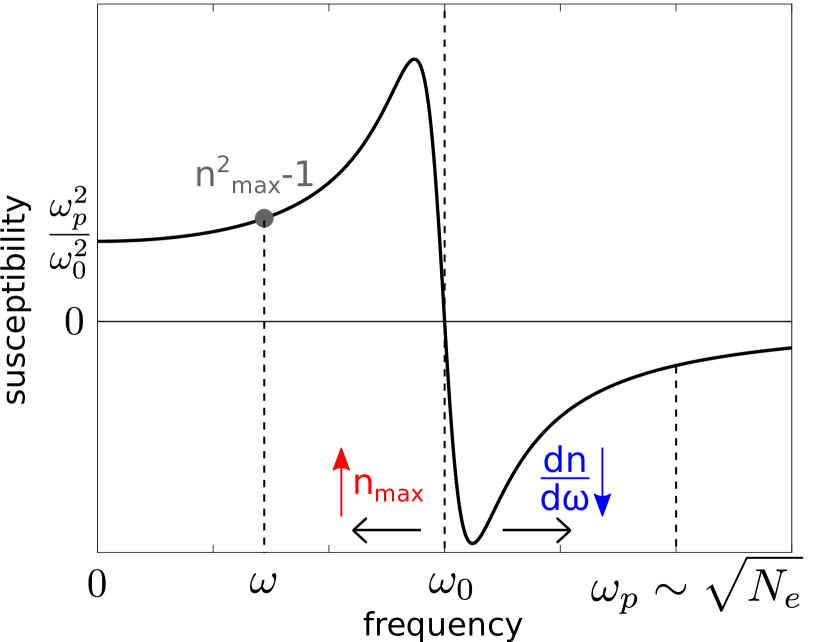
Figure 1: Schematic representation of a single Drude–Lorentz oscillator, depicting the tradeoff between refractive index and dispersion. Decreasing the resonance frequency $\omega_{0}$ increases the ratio $\frac{\omega_{p}^{2}}{\omega_{0}^{2}}$ and hence the maximum refractive index $n_{\textrm{max}}$ at $\omega$, but at the cost of higher dispersion $\frac{{\rm d}n}{{\rm d}\omega}$ (and vice versa for increasing $\omega_{0}$). The plasma frequency $\omega_{p}=\sqrt{\frac{N_{e}e^{2}}{\varepsilon_{0}m_{e}}}$ is determined by the material’s electron density.

II Single-frequency bound

II.1 Fundamental limit

A canonical version of the refractive-index question is: what is the largest possible refractive index of a transparent (lossless) medium, at frequency $\omega$, subject to some maximum allowable dispersion? The dispersion constraint is important for many applications, from metalenses to photovoltaics, where one may want to operate over a reasonable bandwidth or minimize the phase- and/or group-velocity variability that can be difficult to overcome purely by design [89, 90, 91]. Given the susceptibility representation of Eqs. (3,4) in Sec. I, we can formulate the maximum-refractive-index question in terms of the susceptibility, and then transform the optimal solution to a bound on refractive index. We assume here a nonmagnetic medium, in which case we can connect electric susceptibility to refractive index; in Sec. V we show that the same bounds apply even in the presence of magnetic response.

The formulation of this canonical single-frequency refractive-index maximization as a linear program is straightforward. The Kramers–Kronig representation of Eq. (3) can be written as $\chi(\omega)=\sum_{i}c_{i}f_{i}(\omega)$, where $f_{i}$ at frequency $\omega$ is given by $f_{i}(\omega)=\omega_{p}^{2}/(\omega_{i}^{2}-\omega^{2})$ and $\chi(\omega)$ is linear in the $c_{i}$ values. The dispersion, as measured by the frequency derivative of the real part of the susceptibility, has the same representation but with $f_{i}(\omega)$ replaced by its derivative $f_{i}^{\prime}(\omega)=2\omega\omega_{p}^{2}/(\omega_{i}^{2}-\omega^{2})^{2}$. Then, the largest possible susceptibility at frequency $\omega$, with dispersion constrained to be smaller than an application-specific constant $\chi^{\prime}$, is the solution of the optimization problem:

$$\underset{c_{i}}{\text{maximize}} \operatorname{Re}\chi(\omega)=\sum_{i=1}^{N}c_{i}\,f_{i}(\omega)$$ (6)

subject to $$\frac{{\rm d}\operatorname{Re}\chi(\omega)}{{\rm d}\omega}=\sum_{i=1}^{N}c_{i}\,f_{i}^{\prime}(\omega)\leq\chi^{\prime},$$

$$\sum_{i=1}^{N}c_{i}=1,\ c_{i}\geq 0.$$

Equation (6) is of the general linear-program form in Eq. (5). Comparing the two expressions, the vector $z$ has $f_{i}(\omega)$ as its elements. There is only a single index $j$, with matrix $A_{1}$ given by a single column with values $f_{i}^{\prime}(\omega)$ and $b_{1}$ is a vector of 1’s multiplied by $-\chi^{\prime}$. To computationally optimize the maximum-index problem of Eq. (6), one must simply represent a sufficiently large space of possible oscillator frequencies $\omega_{i}$. Since we are interested in transparent (lossless) media, there should not be any oscillator at the frequency of interest $\omega$ (otherwise there will be significant absorption). Nor should there be any oscillator frequencies $\omega_{i}<\omega$, which can only reduce the susceptibility at $\omega$. Thus, one only needs to consider oscillator strengths $\omega_{i}$ greater than $\omega$.

Strikingly, for any frequency $\omega$, electron density $N_{e}$ (or plasma frequency $\omega_{p}$), and allowable dispersion $\chi^{\prime}$, the optimal solution to Eq. (6) is always represented by a single nonzero oscillator, with strength $c_{0}=1$ and frequency $\omega_{0}=\omega\sqrt{1+\sqrt{2\omega_{p}^{2}/(\omega^{3}\chi^{\prime})}}$. We prove in the SM that this single-oscillator solution is globally optimal. The intuition behind the optimality of a single oscillator can be understood from Fig. 1. The susceptibility of a single oscillator is governed by three frequencies: the frequency of interest, $\omega$, the oscillator frequency, $\omega_{0}$, and the electron-density-based plasma frequency, $\omega_{p}$. The static susceptibility of such an oscillator at zero frequency is given by $\chi=\omega_{p}^{2}/\omega^{2}$. This sets a starting point for the susceptibility that ideally should be as large as possible. The plasma frequency is fixed for a given electron density, and thus the only way to increase the static susceptibility is to reduce the oscillator frequency $\omega_{0}$ (as indicated by the black left arrow). Yet this comes with a tradeoff: as $\omega_{0}$ decreases, the oscillator nears the frequency of interest, and the dispersion naturally increases. Hence for minimal dispersion one would want as large of an oscillator frequency as possible. A constraint on allowable dispersion thus imposes a bound on how small of an oscillator frequency one can have, and the maximum refractive index is achieved by concentrating all of the available oscillator strength, determined by the f-sum rule, at that frequency.

The single-oscillator optimality of the solution to Eq. (6) leads to an analytical bound on the maximum achievable refractive index. Denoting a maximal refractive-index dispersion $n^{\prime}=\chi^{\prime}/2n$ (from $\chi=n^{2}-1$), straightforward algebra (cf. SM) leads to a general bound on achievable refractive index:

$$\frac{(n^{2}-1)^{2}}{n}\leq\frac{\omega_{p}^{2}n^{\prime}}{\omega}.$$ (7)

Equation (7) is a key result of our paper, delineating the largest achievable refractive index at any frequency for any passive, linear, isotropic material. Equation (7) highlights the three key determinants of maximum refractive index: electron density, allowable dispersion, and frequency of interest. We will discuss each of these three dependencies in depth. First, though, there is a notable simplification of the refractive-index bound, Eq. (7), when the refractive index is moderately large. In that case, the left-hand side of Eq. (7) is simply the cube of $n$; taking the cube root, we have the high-index ($n^{2}\gg 1$) bound:

$$n\leq\left(\frac{\omega_{p}^{2}n^{\prime}}{\omega}\right)^{1/3}.$$ (8)

The cube-root dependence of the high-index bound, Eq. (8) is a strong constraint: it says that increasing electron density or allowable dispersion by even a factor of 2 will only result in a $\sqrt[3]{2}\approx 1.26\textrm{X}$ enhancement. Similarly, even an order-of-magnitude, 10X increase in either variable can only enhance refractive index by a little more than 2X. Thus the opportunity for significant increases in refractive index are highly limited. The cube-root dependence that is responsible for this constraint is new and surprising: conventional arguments suggest that refractive index should scale with the square root of electron density [87]. Moreover, applying our analysis to the Kramers–Kronig representation of refractive index also leads to square-root scaling. It is the fact that the susceptibilities of nonmagnetic materials, in addition to their refractive indices, must satisfy Kramers–Kronig relations, that ultimately leads to the tighter cube-root dependence, as further discussed in Sec. II.3.

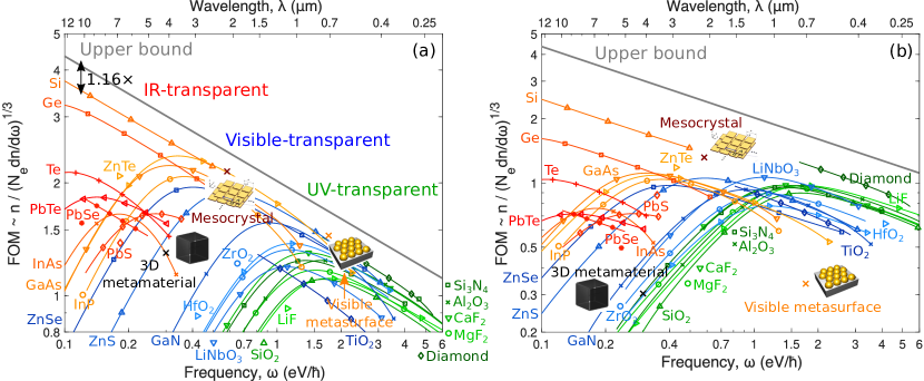
Figure 2: Comparison of representative high-index materials, as well as three metamaterial designs (visible metasurface [48], 3D metamaterial [49], mesocrystal [92]) from the literature, as measured by the FOM = $\left[\frac{(n^{2}-1)^{2}}{n\omega_{p}^{2}n^{\prime}}\right]^{1/3}\approx\frac{n}{N_{e}n^{\prime}}$ for $n\gg 1$ ($N_{e}n^{\prime}$ normalized to that of valence SiO₂ at 400 nm), plotted against the material-independent bound in Eq. (9). Shown above are two figures, based on (a) total and (b) valence electron density, which only shifts the FOM for each material without distorting qualitative features. The materials can be broadly classified into three categories depending on the spectrum at which they are transparent—UV (LiF [93], MgF₂ [93], CaF₂ [93], SiO₂ [94, 95], Al₂O₃ [94, 96], Si₃N₄ [97], diamond [98]), visible (HfO₂ [99], ZrO₂ [100], LiNbO₃ [101], ZnS [102, 103], GaN [104], ZnSe [105], TiO₂ [47]), and IR (ZnTe [106], InP [107], GaAs [108], Si [109], InAs [110], Ge [111], PbS [112], PbSe [112], Te [113, 114], PbTe [115]). Most materials approach the bound quite closely at different frequencies, with silicon at IR outperformed only by a factor of 1.16 relative to the bound. The parabolic shape bending downwards at IR frequencies can be attributed to phonon dispersion, notable exceptions being silicon and germanium, which are IR-inactive and hence highly transparent even in mid-IR (i.e. very non-dispersive).

To investigate the validity of our bounds of Eqs. (7,8), we compare them to the actual refractive indices of a wide range of real materials. To compare the bound to a real material at varying frequencies, we must account for the different electron densities, dispersion values, and frequencies of interest for those materials. To unify the comparisons, we use the bound of Eq. (7) to define a material-dependent refractive-index “figure of merit,”

$$\textrm{FOM}\equiv\left[\frac{(n^{2}-1)^{2}}{n\omega_{p}^{2}n^{\prime}}\right]^{1/3}\leq\frac{1}{\omega^{1/3}}.$$ (9)

which is approximately the refractive index rescaled by powers of the plasma frequency and allowable dispersion. On the right-hand side of Eq. (9) is the factor $1/\omega^{1/3}$, which is the upper bound to the material figure of merit for any material.

Figure 2 compares the material-figure-of-merit bound (solid black line) to the actual material figure of merit for a wide range of materials (colored lines and markers) [93, 94, 95, 96, 97, 98, 99, 100, 101, 102, 103, 104, 105, 47, 106, 107, 108, 109, 110, 111, 112, 113, 114, 115]. We use the experimentally determined refractive indices and dispersion values for each material. Parts (a) and (b) of the figure are identical except for the values of the electron density: in part (b), we use the total electron density of each material, while in part (a) we use only the valence electron density. The valence-electron-density bound is not a rigorous bound, but in practice it is only the valence electrons that contribute to the refractive index at optical frequencies, and one can see that the bound in (a) is tighter than that of (b) due to the use of the valence densities, while not being surpassed by any real materials. Within the materials considered, we use the line and marker colors to distinguish materials that are transparent at infrared (IR), visible, and ultraviolet (UV) frequencies, respectively. The higher the frequency of interest, the lower the material FOM bound is (and the lower the refractive-index bound is), because at higher frequencies the oscillator frequency must increase to prevent the dispersion value from surpassing its limit, and a higher oscillator frequency reduces the electrostatic index that sets a baseline for its ultimate value (as can be seen in Fig. 1).

Three metamaterials structures [49, 48, 92] are included in Fig. 2. These metamaterials are patterned to exhibit anomalously large effective indices (ranging from 5 to 10). Ultimately, these metamaterials are configurations of electrons that effectively respond as a homogeneous medium with some refractive index, and thus they too are subject to the bounds of Eqs. (7,8). Indeed, as shown in Fig. 2, two of the metamaterials approach the valence-electron bound line, but do not surpass it. Their high refractive indices are accompanied by dramatically increased chromatic dispersion.

Many materials can approach the bound over a small window of frequencies where their dispersion is minimal relative to their refractive index. Two outliers are silicon and germanium, which approach the bound across almost all frequencies at which they are transparent. Silicon, for example, has a refractive index ($n=3.4$) that is within 16% of its valence-density-based limit. The key factor underlying their standout performance is a subtle one: the absence of optically active phonon modes. It turns out that optical phonons primarily increase the dispersion of a material’s refractive index without increasing its magnitude. From a bound perspective, this can be understood from the sum rule of Eq. (2). In that sum rule, the total oscillator strength is connected to the electron density of a material, divided by the free-electron mass. Technically, there are additionally terms in the sum rule for the protons and neutrons [116]. However, their respective masses are so much larger than those of electrons that their relative contributions to the sum rule are insignificant. Similarly, because phonons are excitations of the lattice, their contribution to refractive index comes from the proton and neutron sum-rule contributions, and are necessarily insignificant in magnitude at optical frequencies. They can, however, substantially alter the dispersion of the material, and indeed that is quite apparent in the refractive indices of many of the other materials (e.g. GaAs, InP, etc.), which thus tend to fall short of the bounds at many frequencies. This result suggests that ideal high-index materials should not host active optical phonons, which increase dispersion without increasing refractive index.

Material	Electron density	Dispersion $\frac{{\rm d}n}{{\rm d}\omega}$ (eV-1)	Refractive index n	Bound on n
	$N_{e}$ (1023 cm-3)	(averaged over 400–700 nm)
MgF2	4.85	0.0059	1.38	1.58
CaF2	3.92	0.0076	1.43	1.60
SiO2	4.25	0.0112	1.46	1.73
Al2O3	5.67	0.0176	1.77	2.04
Si3N4	4.39	0.0514	2.06	2.48
HfO2	4.65	0.0482	2.13	2.49
ZrO2	4.75	0.0597	2.18	2.63
LiNbO3	4.52	0.1266	2.34	3.12
C (diamond)	7.04	0.0436	2.43	2.74
GaN	3.03	0.1448	2.45	2.97
TiO2	5.11	0.3342	2.72	4.17
Metamaterial	0.59	$\approx$ 4.1	$\approx$ 5.1	$\approx$ 5.7

Table 1: High-index materials transparent over the visible spectrum, showing the (valence) electron density $N_{e}$, dispersion $\frac{{\rm d}n}{{\rm d}\omega}$, refractive index $n$, and upper bound on $n$ for each material. The table shows that refractive index, as well as its bound, increases with dispersion, and that they closely approach the bound. Except for the metamaterial, all the quantities listed above are averaged over 400–700 nm.

Table 1 presents numerical values of valence electron densities, dispersion values, refractive indices, and their bounds for representative materials averaged over the visible spectrum (see SM for more details on bounds for nonzero bandwidth). One can see that for a wide variety of materials [93, 94, 95, 96, 97, 98, 99, 100, 101, 104, 47] and dispersion values, there is a close correspondence between the actual refractive index and the bound, for both natural materials and artificial metamaterials. Taken together, Fig. 2 and Table 1 show that many materials can closely approach their respective bounds, showing little room for improvement at the dispersion values naturally available. These results also cast doubt about the result of [54]: a refractive index of 26 at optical frequencies is an order of magnitude larger than any of the natural materials in Table 1. Because of the cube-root scaling of the bound of Eqs. (7,8), a 10X increase in refractive index requires a 1000-fold increase in electron density or dispersion. Large dispersion would inhibit the possibility for the broadband nature of the result in [54], hence the only remaining possibility is a $\approx 1000X$ increase in electron density. Yet this would be orders of magnitude larger than the largest known electron densities [51]. Hence, our results strongly suggest that the light-bending phenomena of [54] are due to diffractive or nonlinear effects, instead of a linear refractive index.

II.2 Maximum index versus chromatic dispersion

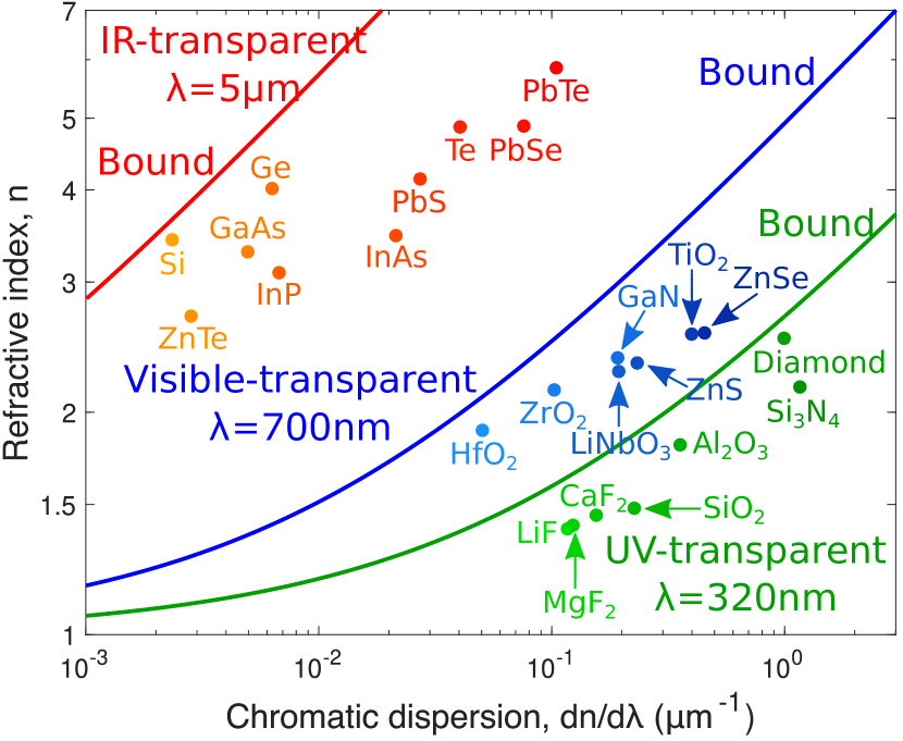
Figure 3: Refractive indices of various materials evaluated at three different wavelengths (320 nm, 500 nm, 5 $\mu$m) based on the spectrum at which they are transparent (UV, visible, and IR respectively), compared to their respective bounds. For each wavelength, the average electron density of all materials belonging to that wavelength was used to compute the bound. The bounds show refractive index increasing with dispersion, as measured by (the magnitude of) chromatic dispersion $\frac{{\rm d}n}{{\rm d}\lambda}$, as also demonstrated by materials closely approaching the bounds.

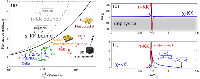
Figure 4: (a) Comparison of bounds based on Kramers–Kronig relations on susceptibility, Eq. (7), and refractive index, Eq. (10), denoted as $n$-KK and $\chi$-KK bound respectively. Natural materials are categorized in terms of the frequencies at which they obtain the highest refractive index (visible, near-IR, and mid-IR, marked as blue, green, and red respectively). All the materials lie below the $\chi$-KK bound. (b) Optimal $\operatorname{Im}\chi$ profiles attaining the $n$-KK and $\chi$-KK bound. Around the resonance frequency $\omega_{0}$, $\operatorname{Im}\chi$ for the former goes negative, which is not allowed by passivity. (c) Optimal $\operatorname{Im}n$ profiles attaining the $n$-KK and $\chi$-KK bound. In contrast to an infinitely sharp resonance for the former, the latter is characterized by a broadened lineshape to the right of $\omega_{0}$. For (b) and (c), the loss rate was taken to be small but nonzero ($\gamma=0.01\omega_{p}$) for purposes of illustration.

To visualize the tradeoff between maximal refractive index and dispersion, Fig. 3 depicts the refractive-index bound of Eq. (7) as a function of chromatic dispersion, for materials transparent at three different wavelengths: infrared ($\lambda=$5\text{\,}\mathrm{u}\mathrm{m}$$), visible ($\lambda=$700\text{\,}\mathrm{n}\mathrm{m}$$), and ultraviolet ($\lambda=$320\text{\,}\mathrm{n}\mathrm{m}$$). We use dispersion with respect to wavelength, i.e. $dn/d\lambda$, instead of frequency, as the wavelength derivative is commonly used in optics [117]. Without careful attention to the wavelength of interest, it would appear that refractive index tends to decrease as dispersion increases: silicon, for example, has both a higher refractive index and smaller dispersion than titanium dioxide, at their respective transparency wavelengths. Yet our bound of Eq. (7) highlights the key role that wavelength is playing in this comparison: the bound shows that maximum index must decrease with increased dispersion but increase at longer wavelengths. Within each color family in Fig. 3, wavelength is held constant, and then it is readily apparent that maximum index increases as a function of chromatic dispersion. One can see that in each wavelength range, many materials are able to approach our bounds across a wide range of dispersion levels. The largest gaps between actual index and that of the bound occur for infrared III-V and II-VI materials, due to the presence of active optical phonons, as discussed above.

At visible and UV frequencies, where phonon contributions are negligible, the deviation of refractive indices from their respective bounds can be attributed to the distributions of oscillator strengths, manifest in the frequency dependence of $\operatorname{Im}\chi(\omega)$. The larger the frequency spread (variance) of $\operatorname{Im}\chi$ relative to its average frequency, the more a material’s refractive index falls short of the bound (cf. SM). Note that for a fixed frequency of interest, the average frequency of the optimal oscillator depends directly on the maximum allowable dispersion: larger dispersion implies smaller oscillator frequency, and vice versa. Hence, higher-dispersion materials have smaller average oscillator frequencies, which reduces the total variance allowed before significant reductions relative to the bounds arise. Diamond would appear to be an exception, but that is only because its valence electron density is much larger than average; its gap to its respective bound is as expected. To summarize: highly dispersive materials are more sensitive to deviations of $\operatorname{Im}\chi(\omega)$ from the ideal delta function than are small-dispersion materials. A direct comparison can be done for TiO₂ and HfO₂, which have similar oscillator spreads but a smaller center frequency for TiO₂. This explains why TiO₂ is farther from its bound than is HfO₂, and explains the general trend of increasing gaps with increasing dispersion.

II.3 Bounds from refractive-index KK relations

In Sec. I, we noted the importance of using Kramers–Kronig relations for the susceptibility instead of KK relations for refractive index. Here, we briefly show the bound that can be derived via refractive-index KK relations, and explain why the two bounds are quite different.

Analogous to the sum rule of Eq. (2), there is a sum rule on the distribution of the imaginary part of refractive index that also scales with the electron density: $\int_{0}^{\infty}\omega\operatorname{Im}n(\omega)\,{\rm d}\omega=\pi\omega_{p}^{2}/4$ ([83]). Similarly, there is a KK relation for refractive index that exactly mimics Eq. (1). Together, following the same mathematical formulation as in Sec. I, one can derive a corresponding bound on refractive index given by (cf. SM):

$$n\leq 1+\frac{\omega_{p}}{2}\sqrt{\frac{n^{\prime}}{\omega}}.$$ (10)

To distinguish the two bounds from each other, we will denote this bound, Eq. (10), as the $n$-KK bound, and the susceptibility-based bound, Eq. (7), as the $\chi$-KK bound. Equation (10) shows that the $n$-KK bound has a square-root dependence on the parameter $\frac{\omega_{p}^{2}n^{\prime}}{\omega}$, in contrast to the cube-root dependence for the $\chi$-KK bound (explicitly shown in Eq. (8) for high-index materials). The $n$-KK bound is always larger than the $\chi$-KK bound (cf. SM), and the square-root versus cube-root dependencies implies that the gap increases with dispersion and electron density. Figure 4(a) shows the difference between the two bounds, and the increasing gap between them at large plasma frequencies or allowable dispersion. Figure 4(b,c) shows the physical origins of the discrepancy between the two approaches. The optimal $n$-KK solution has a delta-function imaginary part of its refractive index, as in Fig. 4(c), concentrating all of the imaginary part in a single refractive-index oscillator. Yet for a delta function in $\operatorname{Im}n$, the imaginary part of the electric susceptibility must go negative in a nonmagnetic material, as in Fig. 4(b), which is unphysical in a passive medium. (At this point, one might wonder if the n-KK bound is achievable by allowing for magnetic response. However, as shown in Sec. V, a non-zero magnetic susceptibility will not help in overcoming the $\chi$-KK bound, as the overall material response under the action of an electromagnetic field is still bound by the $f$-sum rule in Eq. (2).) By contrast, the optimal solution in the $\chi$-KK bound is a delta function in susceptibility, as in Fig. 4(b), which yields a smoother, physical distribution of $\operatorname{Im}n(\omega)$, as seen in Fig. 4(c). Hence another way of understanding the surprising cube-root dependency of our bound is that it arises as a unique consequence of the fact that both refractive index $n$ and its square, $n^{2}=\chi+1$, obey Kramers–Kronig relations [79].

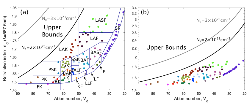
Figure 5: (a) Abbe diagram showing the glasses categorized depending on their refractive indices (at 587.6 nm) $n_{d}$ and Abbe number $V_{d}$, compared to the bounds for electron density $N_{e}=2\times 10^{23}$ cm^-3 (black line) and $N_{e}=3\times 10^{23}$ cm^-3 (gray line). (b) Same plot but shown in logarithmic scale with larger range of values to fully illustrate the bounds. The data for different glass categories was obtained from Ref. [118].

III Bound on optical glasses

The optical glass industry has put significant effort into designing high-index, low-dispersion optical glasses. Thus, transparent optical glasses provide a natural opportunity to test our bounds. It is common practice to categorize refractive indices at specific, standardized wavelengths. The refractive index $n_{d}$ refers to refractive index at the Fraunhofer d spectral line [119], for wavelength $\lambda=$587.6\text{\,}\mathrm{n}\mathrm{m}$$, in the middle of the visible spectrum. Dispersion is measured by the Abbe number $V_{d}$ [120, 121]:

$$V_{d}=\frac{n_{d}-1}{n_{F}-n_{C}},$$ (11)

where $n_{F}$ and $n_{C}$ are evaluated at $486.1\text{\,}\mathrm{n}\mathrm{m}$ and $656.3\text{\,}\mathrm{n}\mathrm{m}$, the Fraunhofer F and C spectral lines, respectively (the Abbe number can be defined differently based on other spectral lines, but the above convention is commonly used to compare optical glasses [122]). The quantity in Eq. (11) cannot be directly constrained in our bound framework, as it is nonlinear in the susceptibility, but optical glasses of interest have sufficiently weak dispersion that their refractive indices can be approximated as linear across the visible spectrum. Then, we can relate the Abbe number directly to the dispersion of the material at $n_{d}$, ${\rm d}n/{\rm d}\omega$, and to the frequency bandwidth between the F and C spectral lines, $\Delta\omega_{FC}$:

$$\frac{{\rm d}n}{{\rm d}\omega}\approx\frac{n_{d}-1}{\Delta\omega_{FC}}\frac{1}{V_{d}}.$$ (12)

which is valid for the wide range of glasses depicted in Fig. 5 with up to only $5\%$ error. Inserting Eq. (12) into the refractive-index bound of Eq. (7), we can write a bound on refractive index in terms of Abbe number $V_{d}$:

$$\frac{(n_{d}^{2}-1)^{2}}{n_{d}(n_{d}-1)}\leq\frac{\omega_{p}^{2}}{\omega_{d}\Delta\omega_{FC}}\frac{1}{V_{d}}.$$ (13)

Figure 5 plots the Abbe diagram [122] of many optical glasses along with our bounds for two representative electron densities, the valence electron density of silicon ($2\times 10^{23}$ cm^-3) and the mean valence electron density of high-index materials shown in Fig. 2 ($3\times 10^{23}$ cm^-3). From Fig. 5(a), there is a striking similarity of the shape of the upper bound and the trendlines for real optical glasses. Moreover, depending on the relevant electron density, the bounds may be quantitatively tight for the best optical glasses. Figure 5(b) zooms out and highlights the high-dispersion (large-Abbe-number) portion of the curve. The trend is very similar to that seen in Fig. 2 earlier: as dispersion increases, the gap between the bound and the refractive index of a real material increases, as the magnitude of the refractive index becomes more sensitive to broadening of the electron oscillator frequencies.

IV Bandwidth-based bound

Instead of constraining the dispersion of a material refractive index, one might similarly require the refractive index to be high over some bandwidth of interest. A first formulation might be to maximize the average refractive index over some bandwidth, but this is ill-posed: an oscillator arbitrarily close to the frequency band of interest can drive the refractive index at the edge of the band arbitrarily high, and the average itself can also diverge. In any case, in a band of potentially large dispersion, the minimum refractive index over the band is the more meaningful metric, as that will be the limiting factor in the desired optical response. Hence, maximizing the minimum refractive index over a bandwidth, i.e., solving a minimax problem, is the well-posed and physically relevant approach. We can pose the corresponding optimization problem problem for some bandwidth $\Delta\omega$ around a center frequency $\omega$ as:

$$\underset{c_{i}}{\text{maximize}} \underset{\omega^{\prime}}{\text{min}}\ \operatorname{Re}\chi(\omega^{\prime})\qquad\omega-\frac{\Delta\omega}{2}\leq\omega^{\prime}\leq\omega+\frac{\Delta\omega}{2}$$ (14)

subject to $$\sum_{i=1}^{N}c_{i}=1,\ c_{i}\geq 0.$$

where again we are considering only a transparency window in which the material is lossless. (As we show in the SM, none of our bounds change substantially if small but nonzero losses are considered.) The solution to Eq. (14) is a single oscillator, analogous to the solution of Eq. (7). In this case, the optimality conditions imply a single oscillator at the frequency $\omega+\Delta\omega/2$, i.e., exactly at the high-frequency edge of the band of interest. This optimal oscillator then implies a fundamental upper limit on the minimum refractive index over bandwidth $\Delta\omega$ around frequency $\omega$ to be (SM):

$$n_{\textrm{min}}\leq\frac{\omega_{p}}{\sqrt{2\omega\Delta\omega}}.$$ (15)

Equation (15) fundamentally constrains how large the minimal refractive index can be over any desired bandwidth. The only extra parameter is the material electron density, as encoded in $\omega_{p}$. The bound increases linearly as the square root of bandwidth $\Delta\omega$ decreases, which can be understood intuitively from the optimal refractive-index profile: decreasing the bandwidth $\Delta\omega$ effectively moves the infinitely sharp resonance (characterized by a delta-function $\operatorname{Im}\chi$) closer to the frequency of interest, thereby shifting the entire refractive-index spectrum upwards and resulting in higher $n_{\textrm{min}}$.

Figure 6 shows the refractive index, normalized by plasma frequency, for representative high-index materials in the visible and UV spectrum (over each of their transparency windows), compared to the bounds for three different bandwidths. Some materials like ZnTe and GaN more closely approach the bounds than others like TiO₂ and HfO₂, which can be traced back to their absorption loss ($\operatorname{Im}\chi$) spectrum. Ideally, the absorption is a delta function situated infinitesimally to the right of the transparency windows for each material, leading to a diverging refractive index at the edge of the transparency window (i.e. the dots for each curve). However, real materials are characterized by broad, smeared-out $\operatorname{Im}\chi$ and thus deviate from the ideal, single Drude–Lorentz response with infinitesimal loss rate. How much each material falls short of the bound signifies to what extent their $\operatorname{Im}\chi$ spectrum is, on average, concentrated away from the frequency of interest. One can deduce from Fig. 6 that, for example, ZnTe is characterized by $\operatorname{Im}\chi$ spectrum focused more towards higher wavelengths relative to TiO₂. The bound of Eq. (15) is more closely approachable for materials with a sharp absorption peak situated as close as possible to the frequency of interest.

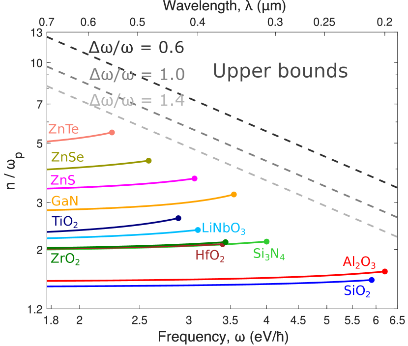
Figure 6: Refractive index normalized by plasma frequency over the UV and visible spectrum, compared to the bounds for three different bandwidths. The dots for each material correspond to the edge of the transparency window, i.e. the frequency beyond which $\operatorname{Im}\chi$ becomes non-negligible. The plasma frequency for each material is normalized to that of SiO₂.

V Bianisotropic media

To this point, we have considered only the refractive indices of isotropic, nonmagnetic media. Although intrinsic magnetism is small at optical frequencies, the fact that patterned metamaterials can exhibit sizeable effective permeabilities suggests the possibility for magnetic response to elevate a metamaterial’s effective refractive index beyond our bounds. More generally, natural and especially artificial materials can demonstrate extreme anisotropy and magneto-electric coupling (chirality) in their response. In this section we consider the most general class of bianisotropic materials, however, and we outline a broad set of conditions under which the refractive-index bounds for such materials are identical to those of Eqs. (7,8) discussed above.

One possibility is to simply use the refractive-index Kramers–Kronig relation and sum rule, as described in Sec. II.3. The refractive index itself allows for magnetism and anisotropy, and thus certainly the bound of Eq. (10) would be valid for each diagonal component of the anisotropic material. Yet it turns out to again be too loose, as we will discuss below. Another possibility would be to consider a magnetic-susceptibility Kramers-Kronig relation and sum rule, in analogy to the electric-susceptibility versions of Eq. (1) and Eq. (2). However, there is no known sum rule on the imaginary part of the magnetic susceptibility. This relates to a deep and fundamental asymmetry between magnetic and electric properties of materials, and to the fact that permeability itself is not a well-defined quantity at very high frequencies [87].

Instead, we exploit the fact that, in macroscopic electrodynamics, any bianisotropic linear material can always be described, equivalently, by purely electric spatially dispersive constitutive relations, as recognized in Refs. [123, 124, 125]. We consider an arbitrary linear, local, bianisotropic medium, with constitutive relation

$$\begin{pmatrix}\mathbf{D}\\ \mathbf{B}\end{pmatrix}=\begin{pmatrix}\overline{\overline{\varepsilon}}&\frac{1}{c}\overline{\overline{\xi}}\\ \frac{1}{c}\overline{\overline{\zeta}}&\overline{\overline{\mu}}\end{pmatrix}\begin{pmatrix}\mathbf{E}\\ \mathbf{H}\end{pmatrix},$$ (16)

where $\overline{\overline{\varepsilon}}$ is permittivity, $\overline{\overline{\mu}}$ is permeability, $\overline{\overline{\xi}}$ and $\overline{\overline{\zeta}}$ are magneto-electric coupling tensors, and $c$ is the speed of light. There is not a unique mapping from the microscopic Maxwell equations in a material (in terms of induced currents in free space) to a macroscopic description in terms of constitutive parameters, as in Eq. (16); in particular, it has been shown that a local, bianisotropic medium is equivalent to a nonlocal, anisotropic, nonmagnetic medium. The nonlocality manifests through a spatially dispersive permittivity that is a function of wavevector $\mathbf{k}$, with the nonlocal effective permittivity given by

$$\overline{\overline{\varepsilon_{\textrm{nl}}}}(\omega,\mathbf{k})= \ \overline{\overline{\varepsilon}}-\overline{\overline{\xi}}\cdot\overline{\overline{\mu}}^{-1}\cdot\overline{\overline{\zeta}}+\left(\overline{\overline{\xi}}\cdot\overline{\overline{\mu}}^{-1}\times\frac{\mathbf{k}}{k_{0}}-\frac{\mathbf{k}}{k_{0}}\times\overline{\overline{\mu}}^{-1}\cdot\overline{\overline{\zeta}}\right)$$

$$+\frac{\mathbf{k}}{k_{0}}\times\left(\overline{\overline{\mu}}^{-1}-\overline{\overline{\mathbf{I}}}\right)\times\frac{\mathbf{k}}{k_{0}},$$ (17)

where $k_{0}=\omega/c$ is the wavenumber in the host medium (taken to be vacuum). In general, Eq. (17) is anisotropic even for isotropic permittivity and/or permeability, due to the wavevector dependence. In this case, we can utilize the fact that Kramers–Kronig relations and the $f$-sum rule are valid for each diagonal component and each individual wavevector of a spatially dispersive, anisotropic medium [126, 125] (cf. SM). We can then represent the nonlocal susceptibility, $\overline{\overline{\chi_{\textrm{nl}}}}(\omega,\mathbf{k})\equiv\overline{\overline{\varepsilon_{\textrm{nl}}}}(\omega,\mathbf{k})-\overline{\overline{I}}$, where $\overline{\overline{I}}$ is the identity tensor, as a sum of lossless Drude–Lorentz oscillators, exactly analogous to Eq. (4). This is because we can always choose a polarization basis for which $\overline{\overline{\chi_{\textrm{nl}}}}(\omega,\mathbf{k})$ is diagonal, since it is Hermitian in the absence of dissipation. (Note that $\overline{\overline{\chi_{\textrm{nl}}}}(\omega,\mathbf{k})$ need not be diagonal for all frequencies $\omega$ and/or wavevectors $\mathbf{k}$ under the same basis. However, we only require that $\overline{\overline{\chi_{\textrm{nl}}}}(\omega,\mathbf{k})$ is diagonalizable at a given frequency and wavevector.)

The refractive index of an anisotropic medium is itself anisotropic, and depends also on the polarization of the electromagnetic field. Consider a propagating plane wave with wavevector $\mathbf{k}=\frac{n\omega}{c}\mathbf{\hat{s}}$. The square of the bianisotropic refractive index, $n_{\rm bianiso}$, experienced by that plane wave is one of two non-trivial solutions of the eigenproblem (cf. Ref. [117], also see SM),

$$\overline{\overline{\varepsilon_{\textrm{nl}}}}(\omega,\mathbf{k})\mathbf{e_{0}}=n_{\textrm{bianiso}}^{2}B\mathbf{e_{0}},$$ (18)

where $B=\overline{\overline{\mathbf{I}}}-\mathbf{\hat{s}}\mathbf{\hat{s}}^{T}$ and $\mathbf{e}_{0}$ is the corresponding eigenvector that physically represents an eigen-polarization. For any material described by a positive- or negative-semidefinite $\overline{\overline{\varepsilon_{\textrm{nl}}}}(\omega,\mathbf{k})$, the square of the refractive index in Eq. (18) is bounded by the largest eigenvalue of $\overline{\overline{\varepsilon_{\textrm{nl}}}}(\omega,\mathbf{k})$ (we defer the discussion of indefinite $\overline{\overline{\varepsilon_{\textrm{nl}}}}(\omega,\mathbf{k})$ to the end of this section). Choosing a polarization basis for which $\overline{\overline{\varepsilon_{\textrm{nl}}}}(\omega,\mathbf{k})$ is diagonal, the largest eigenvalue of $\overline{\overline{\varepsilon_{\textrm{nl}}}}(\omega,\mathbf{k})$ is its largest diagonal component. The magnitude of the diagonal components is bounded by their KK relations and sum rules, which individually degenerate to the isotropic bounds $n_{\rm max,iso}$. (This sequence of steps is mathematically proven in the SM.) Hence, the bianisotropic refractive index is bounded above by the isotropic-material bound:

$$n_{\textrm{bianiso}}\leq n_{\textrm{max},\textrm{iso}}.$$ (19)

Equation (19) says that, no matter how one designs bianisotropic media, its maximum attainable refractive index, for any propagation direction and polarization, can never surpass that of isotropic, electric media, as long as $\overline{\overline{\varepsilon_{\textrm{nl}}}}(\omega,\mathbf{k})$ is positive- or negative-semidefinite. We can intuitively explain why magnetism, chirality, and other bianistropic response cannot help increase the refractive index. Instead of viewing them as distinct phenomena, it is helpful to view them as resulting from the same underlying matter, which can be distributed in different ways to create different induced currents under the action of an applied electromagnetic field. For example, one can tailor the spatial dispersion of permittivity to obtain strong magnetic dipole moments, resulting in effective permeability, or alternatively, create strong chiral response, while the number of available electrons is always the same. Independent of the resulting bianisotropic response, they can all be described by the effective, nonlocal permittivity of Eq. (17) (with varying degrees of spatial dispersion), which is still subject to our upper bound based on the total available electron density. Carrying over our bound techniques employed in Sec. II, the maximal refractive index for such $\overline{\overline{\varepsilon_{\textrm{nl}}}}(\omega,\mathbf{k})$ is therefore identical to Eq. (7) with dispersion corresponding to the maximum principal component of $\overline{\overline{\varepsilon_{\textrm{nl}}}}(\omega,\mathbf{k})$. We show in the SM that most bianisotropic media are captured by positive-definite $\overline{\overline{\varepsilon_{\textrm{nl}}}}(\omega,\mathbf{k})$ and also identify particular conditions (for example, magnetic materials with permeability greater than unity) under which $\overline{\overline{\varepsilon_{\textrm{nl}}}}(\omega,\mathbf{k})$ must be positive definite. Thus, our refractive-index bound is applicable to generic bianisotropic media that describe a wide range of metamaterials. This is a powerful result suggesting that, no matter how one designs metamaterials to include magnetic, chiral, or other bianisotropic response, the tradeoff between refractive index and dispersion is inevitable.

The class of materials that have indefinite material tensors is exactly the class of hyperbolic (meta)materials [127, 128]. In such materials, the bound of Eq. (19) does not apply, and in fact there is no bound that can be derived. Mathematically, this makes sense: the indefinite nature of such materials leads to hyperbolic dispersion curves that can have arbitrarily large wavenumbers at finite frequencies, and consequently refractive indices approaching infinity. Yet, physically, such waves are difficult to access as they are well outside the free-space light cone. Considering more realistic material models, based on microscopic and quantum-plasmonic considerations, this behavior is regularized by the introduction of (i) additional nonlocal effects, e.g., hydrodynamic nonlocalities, which result in a large-wavevector cutoff in the material response [129] and (ii) dissipation (e.g., Landau damping for large wavevectors). An interesting pathway forward would be to use computational optimization, e.g. “inverse design” [130, 131, 132, 133, 91], to identify in-coupling and out-coupling structures that enable access to the high-index modes without reducing the index of the modes themselves.

Another case in which our bound does not hold is for gyrotropic plasmonic materials, the simplest example being a magnetized Drude plasma. Any conducting material has a pole at zero frequency that contributes an additional term in the KK relation for $\operatorname{Im}\chi$, but in gyrotropic plasmonic materials the zero-frequency pole can modify the KK relation for $\operatorname{Re}\chi$, altering Eq. (1) and the subsequent analysis [134]. Due to this additional term in the KK relation for $\operatorname{Re}\chi$, one can attain very large values of permittivity, and hence refractive index, below the cyclotron resonance frequency with low loss and zero dispersion far away from resonance. Yet, such response only occurs below the cyclotron resonance frequency, which is typically much smaller than optical frequencies of interest for technologically available magnetic fields.

VI Designing high-index composites

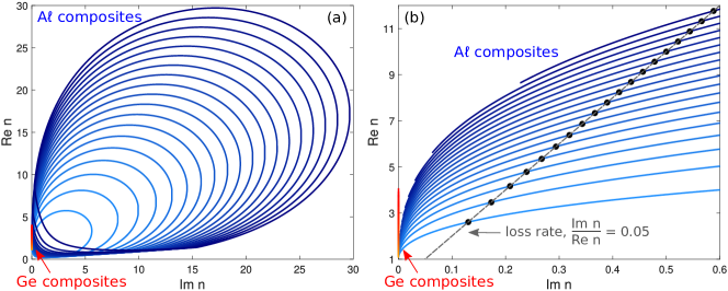
Figure 7: The Bergman–Milton bounds [135, 136], recently strengthened [137], identify the feasible effective material properties of isotropic composite materials (metamaterials). (a) Feasible regions for composites of germanium (red) versus aluminum (blue) at $1550\text{\,}\mathrm{n}\mathrm{m}$ wavelength; in the latter case, each enclosed region represents a different fill fraction of aluminum relative to air. The large, negative susceptibility of aluminum enables strikingly large regions of high index, albeit also with nonzero losses. (b) The low-loss portion of the feasible regions

In the previous sections we showed that for low to moderate dispersion values, natural materials already nearly saturate the fundamental bounds to refractive index. The high-dispersion, high-index part of the fundamental-limit curve has no comparison points, however, as there are no materials that exhibit high dispersion in transparency windows at optical frequencies, and hence no materials exhibit the high refractive indices our bounds suggest should be possible. In fact, renormalization-group principles [58] have been used to identify the maximum refractive index in ensembles of atoms, yielding a value 1.7 that is close to those of real materials. Hence, an important open question is whether it is possible to engineer high refractive index, even allowing for high levels of dispersion?

Here, we show that composite materials can indeed exhibit significantly elevated refractive indices over their natural-material counterparts. Key to the designs is the use of metals and negative-permittivity materials, whose large susceptibilities unlock large positive refractive indices when patterned correctly. We find that with typical metals such as silver and aluminum, it should be possible to reach refractive indices larger than 10, with small losses, at the telecommunications wavelength $1.55\text{\,}\mathrm{\SIUnitSymbolMicro m}$. The lossiness of the metals is the only factor preventing them from reaching even larger values; if it becomes possible to synthesize the “elusive lossless metal” [16], with vanishingly small loss, then properly designed composites can exhibit refractive indices of 100 and beyond.

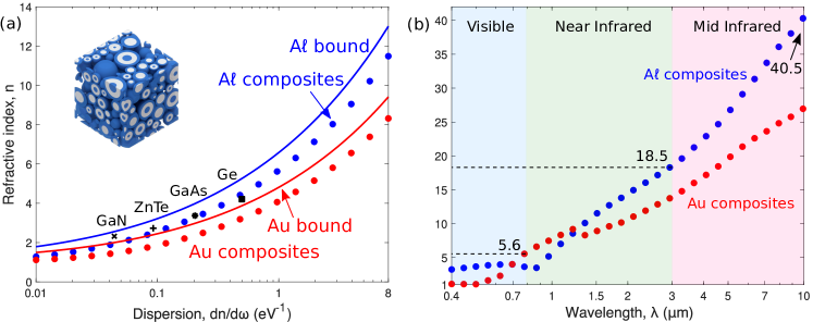
Figure 8: Composites can achieve high refractive indices, at high levels of dispersion, as predicted by our bounds. (a) At $1550\text{\,}\mathrm{n}\mathrm{m}$ wavelength, typical high-index dielectrics such as GaAs and Ge have refractive indices approaching 4. By contrast, assemblages of doubly coated spheres (inset) of gold and aluminum can be designed to achieve low-loss, effective refractive indices above 8 and approaching 12, respectively. Moreover, these composites quite closely approach our bounds (solid lines), suggesting that they are tight or nearly so. (b) Maximum low-loss refractive index of gold and aluminum composites as a function of wavelength. Much higher refractive indices are possible at longer wavelengths, as predicted by our bounds.

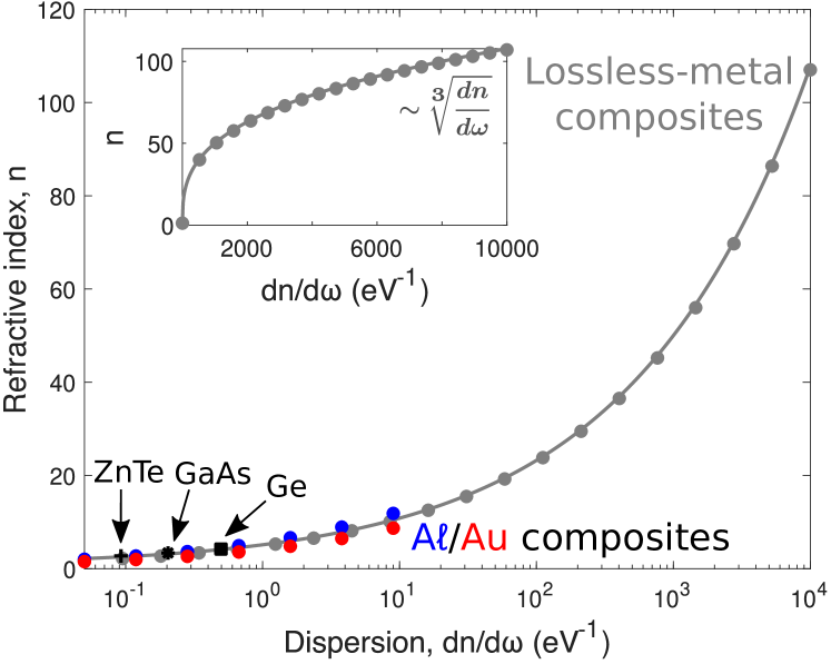
Figure 9: Lower-loss metals would enable even more dramatic enhancements of refractive index. Composites with a nearly lossless metal can be designed to achieve refractive indices larger than 100 at $1550\text{\,}\mathrm{n}\mathrm{m}$ wavelength. These composites (circle markers) exactly achieve our bounds (solid line), and require enormous dispersion values to do so, thanks to the cube-root scaling indicated in the inset.

The theory of composite materials and the effective material properties that can be achieved has been developed over many decades [138, 139]. Composite materials, or metamaterials, comprise multiple materials mixed at highly subwavelength length scales that show effective properties different from those of their underlying constituents. They offer a promising potential route, then, to achieving higher refractive indices through mixing than are possible in natural materials themselves. Bounds, or fundamental limits, to the possible refractive index of an isotropic composite have been known since the pioneering work of Bergman and Milton [135, 136, 140, 141, 142] (and even earlier for lossless materials [143]), and were recently updated and tightened [137]. Bounds are identified as a function of the fill fraction of one of the two (or more) materials. For composite of two materials, the bounds comprise two intersecting arcs in the complex permittivity plane. The analytical expressions for the bounds are given in Eqs. (7,79) of [137], which we do not repeat here due to their modest complexity.

In Fig. 7, we demonstrate what is possible according to the updated Bergman–Milton bounds. At $1550\text{\,}\mathrm{n}\mathrm{m}$ wavelength, we consider two classes of composite, one comprising a higher index dielectric material, germanium, with a low-index material taken to be air, and the second comprising a metallic material, aluminum, with the same air partner. The Ge-based composite exhibits only small variations in its possible refractive index, the red line, occupying the range between 1 (air) and 4.2 (Ge). By contrast, composites with aluminum can exhibit far greater variability, and potentially much larger real parts of their refractive index. The increasingly large regions occupied by the blue arcs represent the bound regions with increasing fill fractions of the aluminum. Of course, one cannot simply choose the highest real refractive index: most of those points are accompanied by tremendously large loss as well. Part (b) of Fig. 7 zooms in on the lower left-hand side of the complex-$n$ plane, where the imaginary parts are sufficiently small that the materials can be considered as nearly lossless. In that region, one can see that there are still sizable possible refractive indices. The largest loss rate can be defined as a ratio of the imaginary part of $n$ to its real part. The real part determines the length over which a $2\pi$ phase accumulation can be achieved, while the imaginary part determines the absorption length, and the key criteria would typically be a large ratio of the two lengths. The black line in Fig. 7(b) represents a loss-rate ratio of $\operatorname{Im}n/\operatorname{Re}n=0.05$. One can see that refractive indices beyond 11 are achievable with an Al-based composite.

It is important to emphasize that the refractive indices shown in Fig. 7(b) are indeed achievable. All of the low-loss bounds shown there, and below, arise from the circular arc that is known to be achievable by assemblages of doubly coated spheres [137]. The inset of Fig. 8(a) schematically shows such an assemblage, comprising densely packed doubly coated spheres that fill all space (cf. Sec. (7.2) of [138]). Figure 8(a) uses circular markers to indicate the largest refractive indices that are possible, as a function of their dispersion values, for doubly-coated-sphere assemblages of aluminum and gold. (Silver is very similar to gold in its possible refractive-index values, due to their similar electron densities.) Accompanying the markers are solid lines that indicate the electron-density-based refractive-index bounds of Eq. (7). One can see that the composites track quite closely with the bounds. Also included are markers for some of the highest-index natural materials, GaN, ZnTe, and GaAs, clearly showing the dramatic extent to which metal-based composites can improve on their natural dielectric counterparts. The figure does not go past dispersion values of $8\text{\,}\mathrm{e}\mathrm{V}^{-1}$, however, as the losses of the composites grow too large in the designs for higher dispersion values. In Fig. 8(b), we map out the largest refractive indices as a function of wavelength that are possible with low-loss composites, with loss rates, as defined above, no larger than 0.05. With such composites, refractive indices larger than 5, 18, and 40 are possible in the visible, near-infrared, and mid-infrared frequency ranges, respectively. Each would represent a record high in its respective frequency range.

The large indices of the Al- and Au-based composites can be increased even further with lower-loss materials. To test the limits of what is possible, in Fig. 9 we consider a composite with a lossless Drude metal with plasma frequency of $10\text{\,}\mathrm{e}\mathrm{V}$ (corresponding to an electron density of 0.7$\times$10²³ cm^-3). The updated BM bound, achieved by the doubly-coated-sphere assemblages, can now exhibit phenomenally large refractive indices, even surpassing 100 in the infrared. As required by our bounds, such refractive indices are accompanied by phenomenally large dispersion values, and the inset shows the slow cube-root increase of refractive index with dispersion for these composites. Our bound of Eq. (7), applied to the Drude material, now lies along the curve for the composites, showing that the composites can saturate our bounds (and, consequently, that our bounds are tight and cannot be further improved.) There is significant interest in engineering lossless metals [16, 17]; if it can be done, we have shown that refractive indices above 100 would be achievable at optical frequencies.

VII Summary and extensions

We have established the maximal refractive index valid for arbitrary passive, linear media, given constraints on dispersion or bandwidth. Starting from Kramers–Kronig relations and the $f$-sum rule that all causal media have to obey, we have obtained a general representation of susceptibility. We have employed linear-programming techniques to demonstrate that the optimal solution is a single Drude–Lorentz oscillator with infinitesimal loss rate, which gave simple, analytic bounds on refractive index. Based on a similar approach, we have obtained bounds on high-index optical glasses and refractive index averaged over arbitrary bandwidth. We have also generalized our bounds to any bianisotropic media described by a positive- or negative-semidefinite effective permittivity $\overline{\overline{\varepsilon_{\textrm{nl}}}}(\omega,\mathbf{k})$, rendering our bounds more general than initially expected (i.e., the maximal refractive indices obtained in Sec. II and Sec. IV also describe materials incorporating magnetic, chiral, and other bianisotropic response). We have also designed low-loss metal-based composites with refractive indices exceeding those of best performing natural materials by a factor of two or more in the high-dispersion regime.

The approach developed herein can be extended to address a variety of related questions. For example, one can allow for gain media, which can still be described by a sum of Drude–Lorentz oscillators with infinitesimal loss rates (see Eq. (4)). However, the oscillator strengths in this scenario need not be positive, leading to different optimal linear-programming solutions depending on the exact objective and constraints. In the case of gain media, stability considerations become crucial, as a high bulk refractive index, or any other bulk property, may be irrelevant, if the resulting structure exhibits an unstable response with unbounded temporal oscillations [144]. Besides, while we have considered optical frequencies in this paper, the bounds established here can be used to compare state-of-the-art dielectrics at microwave and other frequencies of interest. One may also be interested in metrics other than refractive index. A key metric in the context of waveguides and optical fibers is group velocity dispersion [145], which can be seamlessly incorporated into our framework.

Another metric closely related to refractive index is the group index, which measures the reduction in group velocity of electromagnetic waves in a medium. However, unlike refractive index, the group index can reach values up to $60$ even in the near-IR, and much higher elsewhere [31]. This is because group index $n_{g}$, by definition, increases with dispersion:

$$n_{g}=\frac{{\rm d}(n\omega)}{{\rm d}\omega}=n+\omega\frac{{\rm d}n}{{\rm d}\omega}.$$ (20)

Since the first term in Eq. (20) is just the refractive index, which is often of the order of unity, the second term, scaling with dispersion, is usually the dominant term for very large values of group index. That being said, we show in the SM that bounds on group index averaged over arbitrary nonzero bandwidth can be obtained based on our refractive-index bound.

One can also explore negative (anomalous) dispersion, which typically occurs around resonances where losses are sizeable. To do so, one might construct other representations (such as B-splines [146]) that are more suited to describe regions of near-zero or negative dispersion.

An intriguing alternative extension is to nonlinear material properties. There are known Kramers–Kronig relations for nonlinear susceptibilities [147], yet their sum rules [80] are more complex than those of linear susceptibilities. If the sum rules can be simplified, or even just bounded, then it should be possible to identify bounds on nonlinear susceptibilities.

Another avenue that can potentially prove fruitful is to better understand the key characteristics of materials that determine refractive index. While the maximum allowable dispersion sets a limit on refractive index, are there more fundamental, physical quantities at play behind the scene? In the SM, we identify a characteristic trait of high-index materials: a combination of low molar mass and high electronegativity, to achieve large valence electron densities. Going further, it might prove fruitful to combine the insights and directions laid out here with band-structure analysis (through ab-initio methods for example), to extract physical properties conducive to high-index materials.

Finally, direct experimental demonstrations of the high-index materials proposed in Sec. VI would represent record refractive indices. Techniques such as “inverse design” [130, 131, 132, 133, 91] may enable identification of structures with similarly high refractive indices in architectures more amenable to fabrication than assemblages of doubly coated spheres. Identifying such composite materials would open new possibilities in areas from metasurface optics to high-quality-factor resonators. Each of these fields could benefit even more dramatically, potentially, with the discovery or synthesis of a near-zero-loss metal, which, as we have shown, could offer refractive indices approaching 100 at optical frequencies.

VIII Acknowledgments

We thank Christian Kern for providing the illustration of an assemblage of doubly coated spheres. We thank Jacob Khurgin, Michael Fiddy, and Richard Haglund for helpful conversations. H.S. and O.D.M. were supported by the U.S. Defense Advanced Research Projects Agency and Triton Systems. F.M. was supported by the Air Force Office of Scientific Research under Grant FA9550-19-1-0043.

References

- Zheludev and Kivshar [2012] N. I. Zheludev and Y. S. Kivshar, From metamaterials to metadevices, Nature Materials 11, 917 (2012).
- Yu and Capasso [2014] N. Yu and F. Capasso, Flat optics with designer metasurfaces, Nature Materials 13, 139 (2014).
- Lin et al. [2014] D. Lin, P. Fan, E. Hasman, and M. L. Brongersma, Dielectric gradient metasurface optical elements, Science 345, 298 (2014).
- Arbabi et al. [2015] A. Arbabi, Y. Horie, M. Bagheri, and A. Faraon, Dielectric metasurfaces for complete control of phase and polarization with subwavelength spatial resolution and high transmission, Nature Nanotechnology 10, 937 (2015).
- Khorasaninejad et al. [2016] M. Khorasaninejad, W. T. Chen, R. C. Devlin, J. Oh, A. Y. Zhu, and F. Capasso, Metalenses at visible wavelengths: Diffraction-limited focusing and subwavelength resolution imaging, Science 352, 1190 (2016).
- Kuznetsov et al. [2016] A. I. Kuznetsov, A. E. Miroshnichenko, M. L. Brongersma, Y. S. Kivshar, and B. Luk’yanchuk, Optically resonant dielectric nanostructures, Science 354, aag2472 (2016).
- Li et al. [2018] A. Li, S. Singh, and D. Sievenpiper, Metasurfaces and their applications, Nanophotonics 7, 989 (2018).
- Presutti and Monticone [2020] F. Presutti and F. Monticone, Focusing on bandwidth: achromatic metalens limits, Optica 7, 624 (2020).
- Noda et al. [2000] S. Noda, A. Chutinan, and M. Imada, Trapping and emission of photons by a single defect in a photonic bandgap structure, Nature 407, 608 (2000).
- Michler [2000] P. Michler, A Quantum Dot Single-Photon Turnstile Device, Science 290, 2282 (2000).
- Lončar et al. [2003] M. Lončar, A. Scherer, and Y. Qiu, Photonic crystal laser sources for chemical detection, Applied Physics Letters 82, 4648 (2003).
- Reithmaier et al. [2004] J. P. Reithmaier, G. Sȩk, A. Löffler, C. Hofmann, S. Kuhn, S. Reitzenstein, L. V. Keldysh, V. D. Kulakovskii, T. L. Reinecke, and A. Forchel, Strong coupling in a single quantum dot–semiconductor microcavity system, Nature 432, 197 (2004).
- Tanabe et al. [2005] T. Tanabe, M. Notomi, S. Mitsugi, A. Shinya, and E. Kuramochi, All-optical switches on a silicon chip realized using photonic crystal nanocavities, Applied Physics Letters 87, 151112 (2005).
- Hennessy et al. [2007] K. Hennessy, A. Badolato, M. Winger, D. Gerace, M. Atatüre, S. Gulde, S. Fält, E. L. Hu, and A. Imamoğlu, Quantum nature of a strongly coupled single quantum dot–cavity system, Nature 445, 896 (2007).
- Srinivasan and Painter [2007] K. Srinivasan and O. Painter, Linear and nonlinear optical spectroscopy of a strongly coupled microdisk-quantum dot system, Nature 450, 862 (2007).
- Khurgin and Sun [2010] J. B. Khurgin and G. Sun, In search of the elusive lossless metal, Appl. Phys. Lett. 96, 181102 (2010).
- Boltasseva and Atwater [2011] A. Boltasseva and H. A. Atwater, Low-loss Plasmonic Metamaterials, Science 331, 290 (2011).
- Yariv [1989] A. Yariv, Quantum electronics, 3rd ed. (John Wiley & Sons, New York, 1989).
- Yablonovitch [1982] E. Yablonovitch, Statistical Ray Optics., Journal of the Optical Society of America 72, 899 (1982).
- Kerker et al. [1983] M. Kerker, D.-S. Wang, and C. L. Giles, Electromagnetic scattering by magnetic spheres, Journal of the Optical Society of America 73, 765 (1983).
- Schuller et al. [2007] J. A. Schuller, R. Zia, T. Taubner, and M. L. Brongersma, Dielectric Metamaterials Based on Electric and Magnetic Resonances of Silicon Carbide Particles, Physical Review Letters 99, 107401 (2007).
- Ginn et al. [2012] J. C. Ginn, I. Brener, D. W. Peters, J. R. Wendt, J. O. Stevens, P. F. Hines, L. I. Basilio, L. K. Warne, J. F. Ihlefeld, P. G. Clem, and M. B. Sinclair, Realizing Optical Magnetism from Dielectric Metamaterials, Physical Review Letters 108, 097402 (2012).
- Geffrin et al. [2012] J. Geffrin, B. García-Cámara, R. Gómez-Medina, P. Albella, L. Froufe-Pérez, C. Eyraud, A. Litman, R. Vaillon, F. González, M. Nieto-Vesperinas, J. Sáenz, and F. Moreno, Magnetic and electric coherence in forward- and back-scattered electromagnetic waves by a single dielectric subwavelength sphere, Nature Communications 3, 1171 (2012).
- Fu et al. [2013] Y. H. Fu, A. I. Kuznetsov, A. E. Miroshnichenko, Y. F. Yu, and B. Luk’yanchuk, Directional visible light scattering by silicon nanoparticles, Nature Communications 4, 1527 (2013).
- Person et al. [2013] S. Person, M. Jain, Z. Lapin, J. J. Sáenz, G. Wicks, and L. Novotny, Demonstration of zero optical backscattering from single nanoparticles, Nano Letters 13, 1806 (2013).
- Bakker et al. [2015] R. M. Bakker, D. Permyakov, Y. F. Yu, D. Markovich, R. Paniagua-Domínguez, L. Gonzaga, A. Samusev, Y. Kivshar, B. Lukyanchuk, and A. I. Kuznetsov, Magnetic and electric hotspots with silicon nanodimers, Nano Letters 15, 2137 (2015).
- Monticone and Alù [2017] F. Monticone and A. Alù, Scattering at the extreme with metamaterials and plasmonics, in World scientific handbook of metamaterials and plasmonics (World Scientific, 2017) pp. 295–335.
- Vaskin et al. [2018] A. Vaskin, J. Bohn, K. E. Chong, T. Bucher, M. Zilk, D.-Y. Choi, D. N. Neshev, Y. S. Kivshar, T. Pertsch, and I. Staude, Directional and Spectral Shaping of Light Emission with Mie-Resonant Silicon Nanoantenna Arrays, ACS Photonics 5, 1359 (2018).
- Komar et al. [2018] A. Komar, R. Paniagua-Domínguez, A. Miroshnichenko, Y. F. Yu, Y. S. Kivshar, A. I. Kuznetsov, and D. Neshev, Dynamic Beam Switching by Liquid Crystal Tunable Dielectric Metasurfaces, ACS Photonics 5, 1742 (2018).
- Doeleman et al. [2018] H. M. Doeleman, F. Monticone, W. Den Hollander, A. Alù, and A. F. Koenderink, Experimental observation of a polarization vortex at an optical bound state in the continuum, Nature Photonics 12, 397 (2018).
- Baba [2008] T. Baba, Slow light in photonic crystals, Nature Photonics 2, 465 (2008).
- Krauss [2008] T. F. Krauss, Why do we need slow light?, Nature Photonics 2, 448 (2008).
- Robinson et al. [2005] J. T. Robinson, C. Manolatou, L. Chen, and M. Lipson, Ultrasmall Mode Volumes in Dielectric Optical Microcavities, Physical Review Letters 95, 143901 (2005).
- Liang and Johnson [2013] X. Liang and S. G. Johnson, Formulation for scalable optimization of microcavities via the frequency-averaged local density of states, Optics Express 21, 30812 (2013).
- Hu and Weiss [2016] S. Hu and S. M. Weiss, Design of Photonic Crystal Cavities for Extreme Light Concentration, ACS Photonics 3, 1647 (2016).
- Choi et al. [2017] H. Choi, M. Heuck, and D. Englund, Self-Similar Nanocavity Design with Ultrasmall Mode Volume for Single-Photon Nonlinearities, Physical Review Letters 118, 223605 (2017).
- Zhao et al. [2020] Q. Zhao, L. Zhang, and O. D. Miller, Minimum dielectric-resonator mode volumes, arXiv:2008.13241 (2020).
- Nie and Emory [1997] S. Nie and S. R. Emory, Probing single molecules and single nanoparticles by surface-enhanced Raman scattering, Science 275, 1102 (1997).
- Kneipp et al. [1997] K. Kneipp, Y. Wang, H. Kneipp, L. T. Perelman, I. Itzkan, R. R. Dasari, and M. S. Feld, Single Molecule Detection Using Surface-Enhanced Raman Scattering (SERS), Physical Review Letters 78, 1667 (1997).
- van Zanten et al. [2009] T. S. van Zanten, A. Cambi, M. Koopman, B. Joosten, C. G. Figdor, and M. F. Garcia-Parajo, Hotspots of GPI-anchored proteins and integrin nanoclusters function as nucleation sites for cell adhesion, Proceedings of the National Academy of Sciences 106, 18557 (2009).
- Schermelleh et al. [2010] L. Schermelleh, R. Heintzmann, and H. Leonhardt, A guide to super-resolution fluorescence microscopy, Journal of Cell Biology 190, 165 (2010).
- Marcy et al. [1995] H. O. Marcy, L. A. DeLoach, J.-H. Liao, M. G. Kanatzidis, S. P. Velsko, M. J. Rosker, L. F. Warren, C. A. Ebbers, P. H. Cunningham, and C. A. Thomas, l-Histidine tetrafluoroborate: a solution-grown semiorganic crystal for nonlinear frequency conversion, Optics Letters 20, 252 (1995).
- Jain et al. [1996] M. Jain, H. Xia, G. Y. Yin, A. J. Merriam, and S. E. Harris, Efficient Nonlinear Frequency Conversion with Maximal Atomic Coherence, Physical Review Letters 77, 4326 (1996).
- Merriam et al. [2000] A. J. Merriam, S. J. Sharpe, M. Shverdin, D. Manuszak, G. Y. Yin, and S. E. Harris, Efficient nonlinear frequency conversion in an all-resonant double- system, Physical Review Letters 84, 5308 (2000).
- Petrov et al. [2010] V. Petrov, M. Ghotbi, O. Kokabee, A. Esteban-Martin, F. Noack, A. Gaydardzhiev, I. Nikolov, P. Tzankov, I. Buchvarov, K. Miyata, A. Majchrowski, I. Kityk, F. Rotermund, E. Michalski, and M. Ebrahim-Zadeh, Femtosecond nonlinear frequency conversion based on BiB3O6, Laser & Photonics Reviews 4, 53 (2010).
- Li [1980a] H. H. Li, Refractive index of silicon and germanium and its wavelength and temperature derivatives, Journal of Physical and Chemical Reference Data 9, 561 (1980a).
- DeVore [1951] J. R. DeVore, Refractive Indices of Rutile and Sphalerite, Journal of the Optical Society of America 41, 416 (1951).
- Kim et al. [2016] J. Y. Kim, H. Kim, B. H. Kim, T. Chang, J. Lim, H. M. Jin, J. H. Mun, Y. J. Choi, K. Chung, J. Shin, S. Fan, and S. O. Kim, Highly tunable refractive index visible-light metasurface from block copolymer self-assembly, Nature Communications 7, 12911 (2016).
- Shin et al. [2009] J. Shin, J.-T. Shen, and S. Fan, Three-Dimensional Metamaterials with an Ultrahigh Effective Refractive Index over a Broad Bandwidth, Physical Review Letters 102, 093903 (2009).
- Choi et al. [2011] M. Choi, S. H. Lee, Y. Kim, S. B. Kang, J. Shin, M. H. Kwak, K.-Y. Kang, Y.-H. Lee, N. Park, and B. Min, A terahertz metamaterial with unnaturally high refractive index, Nature 470, 369 (2011).
- Kittel and McEuen [1996] C. Kittel and P. McEuen, Introduction to Solid State Physics, vol. 8 ed. (Wiley New York, 1996).
- Lunkenheimer et al. [2009] P. Lunkenheimer, S. Krohns, S. Riegg, S. G. Ebbinghaus, A. Reller, and A. Loidl, Colossal dielectric constants in transition-metal oxides, Eur. Phys. J. Spec. Top. 180, 61 (2009).
- Hu et al. [2013] W. Hu, Y. Liu, R. L. Withers, T. J. Frankcombe, L. Norén, A. Snashall, M. Kitchin, P. Smith, B. Gong, H. Chen, J. Schiemer, F. Brink, and J. Wong-Leung, Electron-pinned defect-dipoles for high-performance colossal permittivity materials, Nat. Mater. 12, 821 (2013).
- Di Mei et al. [2018] F. Di Mei, L. Falsi, M. Flammini, D. Pierangeli, P. Di Porto, A. J. Agranat, and E. DelRe, Giant broadband refraction in the visible in a ferroelectric perovskite, Nature Photonics 12, 734 (2018).
- Moss [1950] T. S. Moss, A Relationship between the Refractive Index and the Infra-Red Threshold of Sensitivity for Photoconductors, Proceedings of the Physical Society. Section B 63, 167 (1950).
- Ravindra et al. [2007] N. Ravindra, P. Ganapathy, and J. Choi, Energy gap–refractive index relations in semiconductors – An overview, Infrared Physics & Technology 50, 21 (2007).
- Jackson [1999] J. D. Jackson, Classical Electrodynamics, 3rd Ed. (John Wiley & Sons, 1999).
- Andreoli et al. [2021] F. Andreoli, M. J. Gullans, A. A. High, A. Browaeys, and D. E. Chang, Maximum refractive index of an atomic medium, Phys. Rev. X 11, 011026 (2021).
- Kuzyk [2000] M. G. Kuzyk, Physical Limits on Electronic Nonlinear Molecular Susceptibilities, Physical Review Letters 85, 1218 (2000).
- Kuzyk [2006] M. G. Kuzyk, Fundamental limits of all nonlinear-optical phenomena that are representable by a second-order nonlinear susceptibility, The Journal of Chemical Physics 125, 154108 (2006).
- Skaar and Seip [2006] J. Skaar and K. Seip, Bounds for the refractive indices of metamaterials, Journal of Physics D: Applied Physics 39, 1226 (2006).
- Gustafsson and Sjöberg [2010] M. Gustafsson and D. Sjöberg, Sum rules and physical bounds on passive metamaterials, New Journal of Physics 12, 043046 (2010).
- Stockman [2007] M. I. Stockman, Criterion for Negative Refraction with Low Optical Losses from a Fundamental Principle of Causality, Physical Review Letters 98, 177404 (2007).
- Milton and Srivastava [2020] G. W. Milton and A. Srivastava, Further comments on Mark Stockman’s article ”Criterion for Negative Refraction with Low Optical Losses from a Fundamental Principle of Causality”, arXiv preprint arXiv:2010.05986 (2020).
- Miller et al. [2016] O. D. Miller, A. G. Polimeridis, M. T. H. Reid, C. W. Hsu, B. G. Delacy, J. D. Joannopoulos, M. Soljačic̀, and S. G. Johnson, Fundamental limits to optical response in absorptive systems, Optics Express 24, 3329 (2016).
- Hugonin et al. [2015] J.-P. Hugonin, M. Besbes, and P. Ben-Abdallah, Fundamental limits for light absorption and scattering induced by cooperative electromagnetic interactions, Physical Review B 91, 180202(R) (2015).
- Miller et al. [2017] O. D. Miller, O. Ilic, T. Christensen, M. T. H. Reid, H. A. Atwater, J. D. Joannopoulos, M. Soljačic̀, and S. G. Johnson, Limits to the optical response of graphene and two-dimensional materials, Nano Letters 17, 5408 (2017).
- Shim et al. [2019] H. Shim, L. Fan, S. G. Johnson, and O. D. Miller, Fundamental Limits to Near-Field Optical Response over Any Bandwidth, Phys. Rev. X 9, 11043 (2019).
- Zhang et al. [2019] H. Zhang, C. W. Hsu, and O. D. Miller, Scattering concentration bounds: Brightness theorems for waves, Optica 6, 1321 (2019).
- Angeris et al. [2019] G. Angeris, J. Vuckovic, and S. P. Boyd, Computational Bounds for Photonic Design, ACS Photonics 6, 1232 (2019).
- Molesky et al. [2019] S. Molesky, W. Jin, P. S. Venkataram, and A. W. Rodriguez, T Operator Bounds on Angle-Integrated Absorption and Thermal Radiation for Arbitrary Objects, Phys. Rev. Lett. 123, 257401 (2019).
- Gustafsson et al. [2020] M. Gustafsson, K. Schab, L. Jelinek, and M. Capek, Upper bounds on absorption and scattering, New Journal of Physics 22, 073013 (2020).
- Molesky et al. [2020a] S. Molesky, P. Chao, W. Jin, and A. W. Rodriguez, Global T operator bounds on electromagnetic scattering: Upper bounds on far-field cross sections, Phys. Rev. Res. 2, 033172 (2020a).
- Trivedi et al. [2020] R. Trivedi, G. Angeris, L. Su, S. Boyd, S. Fan, and J. Vuckovic, Bounds for scattering from absorptionless electromagnetic structures, Phys. Rev. Applied 14, 014025 (2020).
- Molesky et al. [2020b] S. Molesky, P. S. Venkataram, W. Jin, and A. W. Rodriguez, Fundamental limits to radiative heat transfer: Theory, Phys. Rev. B 101, 35408 (2020b).
- Kuang et al. [2020] Z. Kuang, L. Zhang, and O. D. Miller, Maximal single-frequency electromagnetic response, Optica 7, 1746 (2020).
- Kuang and Miller [2020] Z. Kuang and O. D. Miller, Computational bounds to light–matter interactions via local conservation laws, Phys. Rev. Lett. 125, 263607 (2020).
- Vanderbei [2015] R. J. Vanderbei, Linear programming, Vol. 3 (Springer, 2015).
- Nussenzveig [1972] H. M. Nussenzveig, Causality and dispersion relations (Academic Press, 1972).
- Lucarini et al. [2005] V. Lucarini, J. J. Saarinen, K.-E. Peiponen, and E. M. Vartiainen, Kramers-Kronig relations in optical materials research, Vol. 110 (Springer Science & Business Media, 2005).
- Reiche and Thomas [1925] F. Reiche and W. Thomas, Über die Zahl der Dispersionselektronen, die einem stationären Zustande zugeordnet sind. (Vorläufige Mitteilung), Zeitschrift für Physik 34, 510 (1925).
- Kuhn [1925] W. Kuhn, Über die Gesamtstärke der von einem Zustande ausgehenden Absorptionslinien, Zeitschrift für Physik 33, 408 (1925).
- King [1976] F. W. King, Sum rules for the optical constants, J. Math. Phys. 17, 1509 (1976).
- Boyd [2001] J. P. Boyd, Chebyshev and Fourier spectral methods, 2nd ed. (Dover, New York, 2001).
- Cardona and Peter [2005] M. Cardona and Y. Y. Peter, Fundamentals of semiconductors (Springer, 2005).
- Kaxiras and Joannopoulos [2019] E. Kaxiras and J. D. Joannopoulos, Quantum theory of materials (Cambridge university press, 2019).
- Landau et al. [2013] L. D. Landau, J. S. Bell, M. J. Kearsley, L. P. Pitaevskii, E. M. Lifshitz, and J. B. Sykes, Electrodynamics of continuous media, Vol. 8 (Elsevier, 2013).
- Nocedal and Wright [2006] J. Nocedal and S. J. Wright, Numerical Optimization, 2nd ed. (Springer, New York, NY, 2006).
- Genevet et al. [2017] P. Genevet, F. Capasso, F. Aieta, M. Khorasaninejad, and R. Devlin, Recent advances in planar optics: from plasmonic to dielectric metasurfaces, Optica 4, 139 (2017).
- Chen et al. [2018] W. T. Chen, A. Y. Zhu, V. Sanjeev, M. Khorasaninejad, Z. Shi, E. Lee, and F. Capasso, A broadband achromatic metalens for focusing and imaging in the visible, Nature Nanotechnology 13, 220 (2018).
- Chung and Miller [2020] H. Chung and O. D. Miller, High-NA achromatic metalenses by inverse design, Optics Express 28, 6945 (2020).
- Chang et al. [2016] T. Chang, J. U. Kim, S. K. Kang, H. Kim, D. K. Kim, Y.-H. Lee, and J. Shin, Broadband giant-refractive-index material based on mesoscopic space-filling curves, Nature Communications 7, 12661 (2016).
- Li [1980b] H. H. Li, Refractive index of alkaline earth halides and its wavelength and temperature derivatives, Journal of Physical and Chemical Reference Data 9, 161 (1980b).
- Malitson [1965] I. H. Malitson, Interspecimen Comparison of the Refractive Index of Fused Silica, Journal of the Optical Society of America 55, 1205 (1965).
- Tan [1998] C. Tan, Determination of refractive index of silica glass for infrared wavelengths by IR spectroscopy, Journal of Non-Crystalline Solids 223, 158 (1998).
- Weber [1986] M. J. Weber, Handbook of Laser Science and Technology: Volume 4: Optical Mtls, Vol. 4 (CRC-Press, 1986).
- Luke et al. [2015] K. Luke, Y. Okawachi, M. R. E. Lamont, A. L. Gaeta, and M. Lipson, Broadband mid-infrared frequency comb generation in a Si3N4 microresonator, Optics Letters 40, 4823 (2015).
- Peter [1923] F. Peter, Über Brechungsindizes und Absorptionskonstanten des Diamanten zwischen 644 und 226 m, Zeitschrift für Physik 15, 358 (1923).
- Wood et al. [1990] D. L. Wood, K. Nassau, T. Y. Kometani, and D. L. Nash, Optical properties of cubic hafnia stabilized with yttria, Applied Optics 29, 604 (1990).
- Wood and Nassau [1982] D. L. Wood and K. Nassau, Refractive index of cubic zirconia stabilized with yttria, Applied Optics 21, 2978 (1982).
- Zelmon et al. [1997] D. E. Zelmon, D. L. Small, and D. Jundt, Infrared corrected Sellmeier coefficients for congruently grown lithium niobate and 5 mol.% magnesium oxide-doped lithium niobate, Journal of the Optical Society of America B 14, 3319 (1997).
- Debenham [1984] M. Debenham, Refractive indices of zinc sulfide in the 0405–13-m wavelength range, Applied Optics 23, 2238 (1984).
- Klein [1986] C. A. Klein, Room-temperature dispersion equations for cubic zinc sulfide, Applied Optics 25, 1873 (1986).
- Barker and Ilegems [1973] A. S. Barker and M. Ilegems, Infrared Lattice Vibrations and Free-Electron Dispersion in GaN, Physical Review B 7, 743 (1973).
- Amotchkina et al. [2020] T. Amotchkina, M. Trubetskov, D. Hahner, and V. Pervak, Characterization of e-beam evaporated Ge, YbF3 , ZnS, and LaF3 thin films for laser-oriented coatings, Applied Optics 59, A40 (2020).
- Li [1984] H. H. Li, Refractive Index of ZnS, ZnSe, and ZnTe and Its Wavelength and Temperature Derivatives, Journal of Physical and Chemical Reference Data 13, 103 (1984).
- Pettit and Turner [1965] G. D. Pettit and W. J. Turner, Refractive Index of InP, Journal of Applied Physics 36, 2081 (1965).
- Skauli et al. [2003] T. Skauli, P. S. Kuo, K. L. Vodopyanov, T. J. Pinguet, O. Levi, L. A. Eyres, J. S. Harris, M. M. Fejer, B. Gerard, L. Becouarn, and E. Lallier, Improved dispersion relations for GaAs and applications to nonlinear optics, Journal of Applied Physics 94, 6447 (2003).
- Chandler-Horowitz and Amirtharaj [2005] D. Chandler-Horowitz and P. M. Amirtharaj, High-accuracy, midinfrared (450cm 4000cm-1) refractive index values of silicon, Journal of Applied Physics 97, 123526 (2005).
- Lorimor and Spitzer [1965] O. G. Lorimor and W. G. Spitzer, Infrared Refractive Index and Absorption of InAs and CdTe, Journal of Applied Physics 36, 1841 (1965).
- Burnett et al. [2016] J. H. Burnett, S. G. Kaplan, E. Stover, and A. Phenis, Refractive index measurements of Ge, in Infrared Sensors, Devices, and Applications VI, Vol. 9974 (International Society for Optics and Photonics, 2016) p. 99740X.
- Zemel et al. [1965] J. N. Zemel, J. D. Jensen, and R. B. Schoolar, Electrical and Optical Properties of Epitaxial Films of PbS, PbSe, PbTe, and SnTe, Physical Review 140, A330 (1965).
- Caldwell and Fan [1959] R. S. Caldwell and H. Y. Fan, Optical Properties of Tellurium and Selenium, Physical Review 114, 664 (1959).
- Bhar [1976] G. C. Bhar, Refractive index interpolation in phase-matching, Applied optics 15, 305 (1976).
- Weiting and Yixun [1990] F. Weiting and Y. Yixun, Temperature effects on the refractive index of lead telluride and zinc selenide, Infrared Physics 30, 371 (1990).
- Yan and Drake [1995] Z.-c. Yan and G. W. F. Drake, Theoretical lithium 2 2 S→ 2 2 P and 2 2 P→ 3 2 D oscillator strengths, Physical Review A 52, R4316 (1995).
- Born and Wolf [2013] M. Born and E. Wolf, Principles of optics: electromagnetic theory of propagation, interference and diffraction of light (Elsevier, 2013).
- Schott [2011] A. G. Schott, Optical glass data sheets, Retrieved February (2011).
- Hearnshaw [1990] J. B. Hearnshaw, The analysis of starlight: one hundred and fifty years of astronomical spectroscopy (CUP Archive, 1990).
- Hovestadt [1902] H. Hovestadt, Jena Glass: And Its Scientific and Industrial Applications (Macmillan, 1902).
- Bergmann and Schaefer [1999] L. Bergmann and C. Schaefer, Optics of waves and particles (W. de Gruyter, 1999).
- Hartmann et al. [2010] P. Hartmann, R. Jedamzik, S. Reichel, and B. Schreder, Optical glass and glass ceramic historical aspects and recent developments: a Schott view, Applied Optics 49, D157 (2010).
- Agranovich et al. [2004] V. M. Agranovich, Y. R. Shen, R. H. Baughman, and A. A. Zakhidov, Linear and nonlinear wave propagation in negative refraction metamaterials, Physical Review B 69, 165112 (2004).
- Silveirinha [2007] M. G. Silveirinha, Metamaterial homogenization approach with application to the characterization of microstructured composites with negative parameters, Physical Review B 75, 115104 (2007).
- Agranovich and Ginzburg [2013] V. M. Agranovich and V. Ginzburg, Crystal optics with spatial dispersion, and excitons, Vol. 42 (Springer Science & Business Media, 2013).
- Altarelli et al. [1972] M. Altarelli, D. L. Dexter, H. M. Nussenzveig, and D. Y. Smith, Superconvergence and Sum Rules for the Optical Constants, Physical Review B 6, 4502 (1972).
- Poddubny et al. [2013] A. Poddubny, I. Iorsh, P. Belov, and Y. Kivshar, Hyperbolic metamaterials, Nature Photonics 7, 948 (2013).
- Ferrari et al. [2015] L. Ferrari, C. Wu, D. Lepage, X. Zhang, and Z. Liu, Hyperbolic metamaterials and their applications, Progress in Quantum Electronics 40, 1 (2015).
- Yan et al. [2012] W. Yan, M. Wubs, and N. A. Mortensen, Hyperbolic metamaterials: Nonlocal response regularizes broadband supersingularity, Physical Review B - Condensed Matter and Materials Physics 86, 1 (2012).
- Jensen and Sigmund [2011] J. S. Jensen and O. Sigmund, Topology optimization for nano-photonics, Laser Photon. Rev. 5, 308 (2011).
- Miller [2012] O. D. Miller, Photonic Design: From Fundamental Solar Cell Physics to Computational Inverse Design, Ph.D. thesis, University of California, Berkeley (2012).
- Molesky et al. [2018] S. Molesky, Z. Lin, A. Y. Piggott, W. Jin, J. Vucković, and A. W. Rodriguez, Inverse design in nanophotonics, Nature Photonics 12, 659 (2018).
- Phan et al. [2019] T. Phan, D. Sell, E. W. Wang, S. Doshay, K. Edee, J. Yang, and J. A. Fan, High-efficiency, large-area, topology-optimized metasurfaces, Light Sci. Appl. 8, 10.1038/s41377-019-0159-5 (2019).
- Abdelrahman and Monticone [2020] M. I. Abdelrahman and F. Monticone, Broadband and giant nonreciprocity at the subwavelength scale in magnetoplasmonic materials, Physical Review B 102, 155420 (2020).
- Bergman [1980] D. J. Bergman, Exactly Solvable Microscopic Geometries and Rigorous Bounds for the Complex Dielectric Constant of a Two-Component Composite Material, Phys. Rev. Lett. 44, 1285 (1980).
- Milton [1980] G. W. Milton, Bounds on the complex dielectric constant of a composite material, Appl. Phys. Lett. 37, 300 (1980).
- Kern et al. [2020] C. Kern, O. D. Miller, and G. W. Milton, Tight bounds on the effective complex permittivity of isotropic composites and related problems, Phys. Rev. Applied 14, 054068 (2020).
- Milton [2002] G. W. Milton, The Theory of Composites (Cambridge University Press, 2002).
- Milton [2016] G. W. Milton, Extending the Theory of Composites to Other Areas of Science, edited by G. W. Milton (Milton-Patton Publishers, Salt Lake City, UT, 2016).
- Milton [1981a] G. W. Milton, Bounds on the complex permittivity of a two-component composite material, J. Appl. Phys. 52, 5286 (1981a).
- Milton [1981b] G. W. Milton, Bounds on the transport and optical properties of a two-component composite material, J. Appl. Phys. 52, 5294 (1981b).
- Bergman [1981] D. J. Bergman, Bounds for the complex dielectric constant of a two-component composite material, Phys. Rev. B 23, 3058 (1981).
- Hashin and Shtrikman [1962] Z. Hashin and S. Shtrikman, A Variational approach to the theory of the effective magnetic permeability of multiphase materials, J. Appl. Phys. 33, 3125 (1962).
- Nistad and Skaar [2008] B. Nistad and J. Skaar, Causality and electromagnetic properties of active media, Physical Review E - Statistical, Nonlinear, and Soft Matter Physics 78, 1 (2008).
- Okamoto [2006] K. Okamoto, Fundamentals of optical waveguides (Academic press, 2006).
- Ivanenko et al. [2019] Y. Ivanenko, M. Gustafsson, B. L. G. Jonsson, A. Luger, B. Nilsson, S. Nordebo, and J. Toft, Passive approximation and optimization using B-splines, SIAM J. Appl. Math. 79, 436 (2019).
- Boyd [2003] R. W. Boyd, Nonlinear optics (Academic Press, 2003).