MIMO-OFDM Joint Radar-Communications:
Is ICI Friend or Foe?

Abstract

Inter-carrier interference (ICI) poses a significant challenge for OFDM joint radar-communications (JRC) systems in high-mobility scenarios. In this paper, we propose a novel ICI-aware sensing algorithm for MIMO-OFDM JRC systems to detect the presence of multiple targets and estimate their delay-Doppler-angle parameters. First, leveraging the observation that spatial covariance matrix is independent of target delays and Dopplers, we perform angle estimation via the MUSIC algorithm. For each estimated angle, we next formulate the radar delay-Doppler estimation as a joint carrier frequency offset (CFO) and channel estimation problem via an APES (amplitude and phase estimation) spatial filtering approach by transforming the delay-Doppler parameterized radar channel into an unstructured form. To account for the presence of multiple targets at a given angle, we devise an iterative interference cancellation based orthogonal matching pursuit (OMP) procedure, where at each iteration the generalized likelihood ratio test (GLRT) detector is employed to form decision statistics, providing as by-products the maximum likelihood estimates (MLEs) of radar channels and CFOs. In the final step, target detection is performed in delay-Doppler domain using target-specific, ICI-decontaminated channel estimates over time and frequency, where CFO estimates are utilized to resolve Doppler ambiguities, thereby turning ICI from foe to friend. The proposed algorithm can further exploit the ICI effect to introduce an additional dimension (namely, CFO) for target resolvability, which enables resolving targets located at the same delay-Doppler-angle cell. Simulation results illustrate the ICI exploitation capability of the proposed approach and showcase its superior detection and estimation performance in high-mobility scenarios over conventional methods.

Index Terms– OFDM, joint radar-communications, intercarrier interference, APES, CFO estimation.

I Introduction

With the explosive growth of spectrally co-existent radars and communication systems in 5G and beyond wireless networks, joint radar-communications (JRC) strategies have become popular in recent years [2, 3, 4, 5, 6, 7]. A promising approach to practical JRC deployment is to design dual-functional radar-communications (DFRC) systems, which employ a single hardware that can simultaneously perform radar sensing and data transmission with a co-designed waveform [8, 9, 3]. Orthogonal frequency-division multiplexing (OFDM) has been widely investigated as a DFRC waveform due its wide availability in wireless communication systems and its potential to achieve high radar performance [10, 11, 12]. In the literature, estimator design for OFDM radar sensing has been studied in both single-antenna [10, 13, 12] and multiple-input multiple-output (MIMO) [14, 15] settings.

In high-mobility scenarios, such as millimeter-wave (mmWave) vehicular JRC systems [3], Doppler-induced intercarrier interference (ICI) can significantly degrade the performance of OFDM from both radar and communications perspective [16, 17, 18]. Due to lack of guard intervals in frequency domain, Doppler shifts produced by mobile targets can destroy the orthogonality of OFDM subcarriers at the receiver (i.e., the ICI effect) and reduce the dynamic range of radar due to increased side-lobe levels [16]. To improve OFDM radar performance, various ICI mitigation approaches have been recently proposed [13, 17, 19, 20]. Considering a single-target scenario, a two-step Doppler estimation method is proposed in [17], where transmit sequences with favorable correlation properties are employed to eliminate ICI. In a similar fashion, the studies in [20, 19] design ICI compensation schemes for a single target relying on the condition that transmit symbols consist of phase codes with certain characteristics regarding cyclic shifts and auto-correlation. As a step further, the work in [13] assumes arbitrary phase shift keying (PSK) symbols and proposes a pulse compression technique to compensate for ICI-induced phase rotations across OFDM subcarriers created by a single target, which can compensate for Doppler shifts at integer multiples of subcarrier spacing. In all of the above schemes, the common observation is that ICI can be harnessed to resolve Doppler ambiguity of a single target.

To tackle the more practical scenarios of multiple targets, recent works investigate range-velocity estimation techniques for multiple objects in the presence of ICI [16, 12, 21]. Under the assumption that the number of targets is known a-priori, an alternating maximization approach that takes ICI into account is proposed in [12] to reduce the complexity of high-dimensional maximum-likelihood (ML) search. In [16], the ICI effect is eliminated via an all-cell Doppler correction (ACDC) method, which performs Doppler compensation for arbitrary velocities with a precision on the level of Doppler resolution. Following a similar line of reasoning, the work in [21] develops a sparsity based ICI removal and range-velocity estimation algorithm. For proper functioning of the methods in [16, 21] in terms of ICI compensation, a common requirement is that OFDM symbol matrix should be rank-one (i.e., same symbols repeated over time).

The prior approaches to OFDM radar sensing in the presence of ICI [17, 19, 20, 16, 12, 21] suffer from several major drawbacks that can significantly limit their applicability in practical JRC scenarios. First, most of the existing ICI compensation methods focus exclusively on the radar functionality of OFDM and impose strict constraints on transmit data symbols, such as cyclic shift property [19], good correlation characteristics [17, 19], identical sequences across subcarriers [20] and rank-one frequency-time OFDM symbol matrix [16, 21]. Such constraints, however, would lead to a substantial loss in communications data rate (e.g., $M$ times reduction in data rate [16, 21], where $M$ is the number of OFDM symbols) and essentially impede dual-functional operation, which is one of the core properties of OFDM. In addition, prior works either focus on a single-target scenario [17, 19, 20], which is not realistic, or study multi-target cases with the assumption that targets have already been detected [12], without addressing the problem of detection under strong ICI, which is challenging due to high side-lobe levels. Moreover, all the existing studies investigate the ICI effect in single-input single-output (SISO) OFDM radar configurations; hence, potential benefits that can be provided by a MIMO-OFDM architecture in tackling the ICI problem have been unexplored. Finally, exploitation of ICI has been considered only in scenarios with limited practical relevance (e.g., containing a single target, with restricted transmit symbols [13, 17, 19, 20]). In a general multi-target setting, ICI conveys crucial information on target velocities and must be exploited to enhance radar performance. In light of the existing literature on OFDM radar sensing under the effect of ICI, three fundamental questions arise:

• How can ICI effect be mitigated in a generic multi-target scenario with arbitrary transmit data symbols, without hampering the communication capability of the OFDM waveform (i.e., no restrictions on data symbols)?

• In what ways can ICI be exploited to improve radar performance in a multi-target scenario?

• How can we best leverage MIMO architectures to design ICI-aware multi-target detection/estimation schemes?

With the goal of answering these questions, this paper tackles the problem of radar sensing with MIMO-OFDM DFRC systems in the presence of non-negligible ICI generated by high-speed targets. Motivated by high-mobility mmWave vehicular applications [3], our goal is to simultaneously mitigate and exploit ICI associated with multiple targets while retaining the communication functionality of OFDM. Towards that goal, we establish a novel method for ICI-aware sensing in MIMO-OFDM DFRC systems, considering arbitrary transmit symbols in multi-target scenarios. Specifically, we propose an ICI-aware multi-target detection and delay-Doppler-angle estimation algorithm for radar sensing by developing an APES-like spatial filtering approach [22], coupled with a generalized likelihood ratio test (GLRT) detection procedure. The key idea is to re-formulate radar sensing as a joint carrier frequency offset (CFO) and channel estimation problem, which allows us to decontaminate the ICI effect from the resulting channel estimates, leading to improved performance in target detection and delay-Doppler estimation. Regarding the ICI exploitation aspect, the proposed algorithm enables accurate estimation of any practically relevant unambiguous velocity that well exceeds the standard maximum limit (e.g., in [10, 23]) determined by OFDM symbol duration, thereby effectively turning ICI from foe to friend. The main contributions can be summarized as follows:

• Novel Formulation of ICI-aware Sensing as Communication Channel/CFO Estimation Problem: We establish an insightful duality between ICI-aware sensing in OFDM radar and joint channel/CFO estimation in OFDM communications [18, 24]. This enables us to formulate the radar delay-Doppler estimation as a joint channel and CFO estimation problem by transforming the delay-Doppler parameterized radar channel into an unstructured form. The key advantage of this novel formulation is that it can produce almost ICI-free channels specific to each target by decoupling ICI compensation from the subsequent delay-Doppler estimation.

• ICI-aware Multi-Target Detector/Estimator Design: Based on the new problem formulation, we design a three-step ICI-aware multi-target detector/estimator. Observing that spatial covariance matrix does not depend on target delays and Dopplers, we first perform angle estimation using the MUSIC high-resolution direction finding algorithm [25]. Next, to suppress mutual multi-target interferences [26] in the spatial domain, we propose a spatial filtering approach stemming from [22] that performs joint CFO/channel estimation and beamforming design for each estimated target angle separately. To take into account the presence of multiple targets at a given angle, we devise an orthogonal matching pursuit (OMP) procedure that implements iterative interference cancellation, whereby at each iteration the strongest echo is detected via GLRT and its effect is subtracted from the received signal. As a by-product, the GLRT detector provides the ML estimates (MLEs) of radar channel and CFO associated to the strongest target in the corresponding iteration. In the final step of the algorithm, detection and delay-Doppler estimation can be performed using target-specific channel estimates (decontaminated from ICI) by exploiting the OFDM time-frequency structure.

• ICI Exploitation: The proposed algorithm exploits the ICI information (obtained as CFO estimates at the output of the second step) in two different ways. First, CFO estimates provide unambiguous target velocities not restricted by OFDM symbol duration, which allows us to resolve velocity ambiguity. Second, we lift the dimension of target resolvability by introducing a fourth dimension (CFO) that allows for distinguishing among targets located at the same delay-Doppler-angle cell.

Additionally, extensive simulations carried out under a wide range of signal-to-noise ratios (SNRs) and target velocities show that the proposed approach provides substantial performance improvements over the conventional FFT based method [10, 23] and achieves performance very close to that obtained by using ICI-free radar observations, in terms of detection and range-velocity estimation accuracy, which demonstrates its superior ICI suppression capability. Furthermore, illustrative examples are presented to reveal the ICI exploitation property of the proposed algorithm.

II OFDM Radar System Model

Consider an OFDM DFRC transceiver that communicates with an OFDM receiver while concurrently performing radar sensing using the backscattered signals for target detection [10, 8]. The DFRC transceiver is equipped with an $N_{\rm{T}}$-element transmit (TX) uniform linear array (ULA) and an $N_{\rm{R}}$-element receive (RX) ULA. We assume co-located and perfectly decoupled TX/RX antenna arrays so that the radar receiver does not suffer from self-interference due to full-duplex radar operation [27, 10, 28, 29, 30]. In this section, we derive OFDM transmit and receive signal models, and formulate the multi-target detection and parameter estimation problem.

II-A Transmit Signal Model

We consider an OFDM communication frame consisting of $M$ OFDM symbols, each of which has a total duration of $T_{\rm{sym}}=T_{\rm{cp}}+T$ and a total bandwidth of $N\Delta f=B$. Here, $T_{\rm{cp}}$ and $T$ denote, respectively, the cyclic prefix (CP) duration and the elementary symbol duration, $\Delta f=1/T$ is the subcarrier spacing, and $N$ is the number of subcarriers [10]. Then, the complex baseband transmit signal for the ${m^{\rm{th}}}$ symbol is given by

$$s_{m}(t)=\frac{1}{\sqrt{N}}\sum_{n=0}^{N-1}x_{n,m}\,e^{j2\pi n\Delta ft}{\rm{rect}}\left(\frac{t-mT_{\rm{sym}}}{T_{\rm{sym}}}\right)$$ (1)

where $x_{n,m}$ denotes the complex data symbol on the ${n^{\rm{th}}}$ subcarrier for the ${m^{\rm{th}}}$ symbol [11], and ${\rm{rect}}\left(t\right)$ is a rectangular function that takes the value $1$ for $t\in\left[0,1\right]$ and $0$ otherwise. Assuming a single-stream beamforming model [29, 14, 31], the transmitted signal over the block of $M$ symbols for $t\in\left[0,MT_{\rm{sym}}\right]$ can be written as

$$\Re\left\{\mathbf{f}_{\rm{T}}\sum_{m=0}^{M-1}s_{m}(t)e^{j2\pi f_{c}t}\right\}$$ (2)

where $f_{c}$ and $\mathbf{f}_{\rm{T}}\in\mathbb{C}^{N_{\rm{T}}\times 1}$ denote, respectively, the carrier frequency and the TX beamforming vector.

II-B Receive Signal Model

Suppose there exists a point target in the far-field, characterized by a complex channel gain $\alpha$ (including path loss and radar cross section effects), an azimuth angle $\theta$, a round-trip delay $\tau$ and a normalized Doppler shift $\nu=2v/c$ (leading to a time-varying delay $\tau(t)=\tau-\nu t$), where $v$ and $c$ denote the radial velocity and speed of propagation, respectively. In addition, let $\mathbf{a}_{\rm{T}}(\theta)\in\mathbb{C}^{N_{\rm{T}}\times 1}$ and $\mathbf{a}_{\rm{R}}(\theta)\in\mathbb{C}^{N_{\rm{R}}\times 1}$ denote, respectively, the steering vectors of the TX and RX ULAs, i.e.,

$$\mathbf{a}_{\rm{T}}(\theta) ={\left[1,e^{j\frac{2\pi}{\lambda}d\sin(\theta)},\ldots,e^{j\frac{2\pi}{\lambda}d(N_{\rm{T}}-1)\sin(\theta)}\right]}^{T}\leavevmode\nobreak\ ,$$ (3)

$$\mathbf{a}_{\rm{R}}(\theta) ={\left[1,e^{j\frac{2\pi}{\lambda}d\sin(\theta)},\ldots,e^{j\frac{2\pi}{\lambda}d(N_{\rm{R}}-1)\sin(\theta)}\right]}^{T}\leavevmode\nobreak\ ,$$ (4)

where $\lambda$ and $d=\lambda/2$ denote the signal wavelength and antenna element spacing, respectively. Given the transmit signal model in (2), the backscattered signal impinging onto the ${i^{\rm{th}}}$ element of the radar RX array can be expressed as

$$y_{i}(t)=\alpha\left[\mathbf{a}_{\rm{R}}(\theta)\right]_{i}\mathbf{a}_{\rm{T}}^{T}(\theta)\mathbf{f}_{\rm{T}}\sum_{m=0}^{M-1}s_{m}\big{(}t-\tau(t)\big{)}e^{-j2\pi f_{c}\tau}e^{j2\pi f_{c}\nu t}.$$

We make the following standard assumptions: (i) the CP duration is larger than the round-trip delay of the furthermost target, i.e., $T_{\rm{cp}}\geq\tau$, [13, 28, 3], (ii) the Doppler shifts satisfy $\lvert\nu\rvert\ll 1/N$ [13, 12], and (iii) the time-bandwidth product (TBP) $BMT_{\rm{sym}}$ is sufficiently low so that the wideband effect can be ignored, i.e., $s_{m}(t-\tau(t))\approx s_{m}(t-\tau)$ [16]. Under this setting, sampling $y_{i}(t)$ at $t=mT_{\rm{sym}}+T_{\rm{cp}}+\ell T/N$ for $\ell=0,\ldots,N-1$ (i.e., after CP removal for the ${m^{\rm{th}}}$ symbol) and neglecting constant terms, the time-domain signal received by the ${i^{\rm{th}}}$ antenna in the ${m^{\rm{th}}}$ symbol can be written as [12]

$$y_{i,m}[\ell] =\alpha\left[\mathbf{a}_{\rm{R}}(\theta)\right]_{i}\mathbf{a}_{\rm{T}}^{T}(\theta)\mathbf{f}_{\rm{T}}\,e^{j2\pi f_{c}mT_{\rm{sym}}\nu}e^{j2\pi f_{c}T\frac{\ell}{N}\nu}$$ (5)

$$\leavevmode\nobreak\ \leavevmode\nobreak\ \times\frac{1}{\sqrt{N}}\sum_{n=0}^{N-1}x_{n,m}\,e^{j2\pi n\frac{\ell}{N}}e^{-j2\pi n\Delta f\tau}\leavevmode\nobreak\ .$$

II-C Fast-Time/Slow-Time Representation with ICI

For the sake of convenience, let us define, respectively, the frequency-domain and temporal steering vectors and the ICI phase rotation matrix as

$$\mathbf{b}(\tau) \triangleq{\left[1,e^{-j2\pi\Delta f\tau},\ldots,e^{-j2\pi(N-1)\Delta f\tau}\right]}^{T}\leavevmode\nobreak\ ,$$ (6)

$$\mathbf{c}(\nu) \triangleq{\left[1,e^{-j2\pi f_{c}T_{\rm{sym}}\nu},\ldots,e^{-j2\pi f_{c}(M-1)T_{\rm{sym}}\nu}\right]}^{T}\leavevmode\nobreak\ ,$$ (7)

$$\mathbf{D}(\nu) \triangleq{\rm{diag}}\left(1,e^{j2\pi f_{c}\frac{T}{N}\nu},\ldots,e^{j2\pi f_{c}\frac{T(N-1)}{N}\nu}\right)\leavevmode\nobreak\ .$$ (8)

Accordingly, the radar observations in (5) can be expressed as

$$\mathbf{y}_{i,m} =\alpha\,\left[\mathbf{a}_{\rm{R}}(\theta)\right]_{i}\mathbf{a}_{\rm{T}}^{T}(\theta)\mathbf{f}_{\rm{T}}\mathbf{D}(\nu)\mathbf{F}_{N}^{H}\Big{(}\mathbf{x}_{m}\odot\mathbf{b}(\tau)\left[\mathbf{c}^{*}(\nu)\right]_{m}\Big{)}$$ (9)

where $\mathbf{F}_{N}\in\mathbb{C}^{N\times N}$ is the unitary DFT matrix with $\left[\mathbf{F}_{N}\right]_{\ell,n}=\frac{1}{\sqrt{N}}e^{-j2\pi n\frac{\ell}{N}}$, $\mathbf{y}_{i,m}\triangleq\left[y_{i,m}[0]\,\ldots\,y_{i,m}[N-1]\right]^{T}$ and $\mathbf{x}_{m}\triangleq\left[x_{0,m}\,\ldots\,x_{N-1,m}\right]^{T}$.

Aggregating (9) over $M$ symbols and considering the presence of multiple targets and noise, the OFDM radar signal received by the ${i^{\rm{th}}}$ antenna over a frame can be written in a fast-time/slow-time compact matrix form as

$$\mathbf{Y}_{i}=\sum_{k=0}^{K-1}\alpha^{(i)}_{k}\underbrace{\mathbf{D}(\nu_{k})}_{\begin{subarray}{c}\rm{ICI}\end{subarray}}\mathbf{F}_{N}^{H}\Big{(}\mathbf{X}\odot\mathbf{b}(\tau_{k})\mathbf{c}^{H}(\nu_{k})\Big{)}+\mathbf{Z}_{i}$$ (10)

for $i=0,\ldots,N_{\rm{R}}-1$, where

$$\alpha^{(i)}_{k} \triangleq\alpha_{k}\,\left[\mathbf{a}_{\rm{R}}(\theta_{k})\right]_{i}\mathbf{a}_{\rm{T}}^{T}(\theta_{k})\mathbf{f}_{\rm{T}}\leavevmode\nobreak\ ,$$ (11)

$$\mathbf{Y}_{i} \triangleq[\mathbf{y}_{i,0}\,\ldots\,\allowbreak\mathbf{y}_{i,M-1}]\in\mathbb{C}^{N\times M}\leavevmode\nobreak\ ,$$ (12)

$$\mathbf{X} \triangleq\left[\mathbf{x}_{0}\,\ldots\,\mathbf{x}_{M-1}\right]\in\mathbb{C}^{N\times M}\leavevmode\nobreak\ ,$$ (13)

$\{\alpha_{k},\tau_{k},\nu_{k},\theta_{k}\}$ are the parameters of the ${k^{\rm{th}}}$ target and $\mathbf{Z}_{i}\in\mathbb{C}^{N\times M}$ is the additive noise matrix with ${\rm{vec}}\left(\mathbf{Z}_{i}\right)\sim{\mathcal{CN}}({{\bm{0}}},\allowbreak\sigma^{2}{\bm{\mathrm{I}}})$.

In (10), each column contains fast-time samples within a particular symbol and each row contains slow-time samples at a particular range bin. The diagonal phase rotation matrix $\mathbf{D}(\nu)$ quantifies the ICI effect in fast-time domain, leading to Doppler-dependent phase-shifts across fast-time samples of each OFDM symbol, similar to the CFO effect in OFDM communications [32, 33]. With this relation to OFDM communications in mind, the parameter $\nu$ in $\mathbf{D}(\nu)$ is often referred to as CFO throughout the text to make a clear distinction between the effects induced by $\nu$ via fast-time phase rotations in $\mathbf{D}(\nu)$ and via slow-time phase rotations in $\mathbf{c}(\nu)$. To visualize the effect of ICI, Fig. 1 illustrates the range profile of an OFDM radar, obtained using a standard FFT based method [10, 23]. It is seen that ICI manifests itself in the range profile as increased side-lobe levels, degrading detection performance.

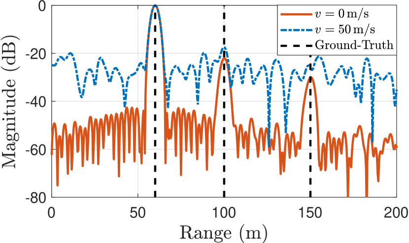
Figure 1: Range profiles of OFDM radar with the parameters given in Table I for two different target velocities. The scenario contains $3$ targets having the same velocity $v$, the ranges $(60,100,150)\,\rm{m}$, the angles $(25^{\circ},30^{\circ},35^{\circ})$ and the SNRs (i.e., $\lvert\alpha_{k}\rvert^{2}/\sigma^{2}$) $(30,5,0)\,\rm{dB}$, respectively. In high-mobility scenarios, ICI reduces the dynamic range of OFDM radar due to increased side-lobe levels and causes masking of weak targets.

II-D Problem Statement for OFDM Radar Sensing

Given the transmit data symbols $\mathbf{X}$, the problem of interest for OFDM radar sensing is to detect the presence of (possibly) multiple targets and estimate their parameters, i.e., channel gains $\{\alpha_{k}\}_{k=0}^{K-1}$, angles $\{\theta_{k}\}_{k=0}^{K-1}$, delays $\{\tau_{k}\}_{k=0}^{K-1}$ and Doppler shifts $\{\nu_{k}\}_{k=0}^{K-1}$, from the received $N_{\rm{R}}\times N\times M$ space/fast-time/slow-time data cube $\{\mathbf{Y}_{i}\}_{i=0}^{N_{\rm{R}}-1}$ in (10).

III ICI-Aware Parameter Estimation via APES Spatial Filtering

In this section, we propose an ICI-aware delay-Doppler-angle estimation algorithm to tackle the sensing problem formulated in Sec. II-D. For ease of exposition, we assume the existence of at most a single target at each azimuth cell. In Sec. IV, relying on this approach, we will develop an algorithm that can detect multiple targets at a given angle and estimate their parameters. Hence, this section serves as a gentle introduction to the core idea of the paper, which will later be complemented by rigorous detection schemes in Sec. IV. In the following, we elaborate on the different steps of the proposed algorithm (see Fig. 2).

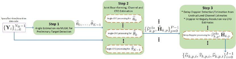
Figure 2: The proposed three-step ICI-aware detector/estimator.

III-A Step 1: Angle Estimation via MUSIC for Preliminary Target Detection

In the first step, we wish to identify a set of angles where potential targets may reside so that receive beamformers can be designed accordingly in the subsequent step. For mathematical convenience, we consider the space/fast-time snapshot of the data cube in (10) corresponding to the ${m^{\rm{th}}}$ OFDM symbol:

$$\macc@depth\char 1\relax\frozen@everymath{\macc@group}\macc@set@skewchar\macc@nested@a 111{\mathbf{Y}} \triangleq\left[\mathbf{y}_{0,m}\,\ldots\,\mathbf{y}_{N_{\rm{R}}-1,m}\right]\in\mathbb{C}^{N\times N_{\rm{R}}}$$ (14)

$$=\sum_{k=0}^{K-1}\alpha_{k}\,\mathbf{a}_{\rm{T}}^{T}(\theta_{k})\mathbf{f}_{\rm{T}}\mathbf{D}(\nu_{k})\mathbf{F}_{N}^{H}{\rm{diag}}\left(\mathbf{x}_{m}\right)$$

$$\leavevmode\nobreak\ \leavevmode\nobreak\ \leavevmode\nobreak\ \leavevmode\nobreak\ \leavevmode\nobreak\ \leavevmode\nobreak\ \leavevmode\nobreak\ \leavevmode\nobreak\ \times\mathbf{b}(\tau_{k})\left[\mathbf{c}^{*}(\nu_{k})\right]_{m}\mathbf{a}_{\rm{R}}^{T}(\theta_{k})+\macc@depth\char 1\relax\frozen@everymath{\macc@group}\macc@set@skewchar\macc@nested@a 111{\mathbf{Z}}_{m}$$

for $m=0,\ldots,M-1$, where $\macc@depth\char 1\relax\frozen@everymath{\macc@group}\macc@set@skewchar\macc@nested@a 111{\mathbf{Z}}_{m}\in\mathbb{C}^{N\times N_{\rm{R}}}$ is the noise component distributed according to ${\rm{vec}}\left(\macc@depth\char 1\relax\frozen@everymath{\macc@group}\macc@set@skewchar\macc@nested@a 111{\mathbf{Z}}_{m}\right)\sim{\mathcal{CN}}({{\bm{0}}},\allowbreak\sigma^{2}{\bm{\mathrm{I}}})$. To distinguish targets with high resolution in the angular domain using small number of antennas (in compliance with mmWave automotive radar requirements [6]), we propose to perform angle estimation using the MUSIC algorithm [25]. To this end, we first construct the spatial covariance matrix (SCM) of the data cube in (14) as

$$\mathbf{R}\triangleq\sum_{m=0}^{M-1}\macc@depth\char 1\relax\frozen@everymath{\macc@group}\macc@set@skewchar\macc@nested@a 111{\mathbf{Y}}_{m}^{H}\macc@depth\char 1\relax\frozen@everymath{\macc@group}\macc@set@skewchar\macc@nested@a 111{\mathbf{Y}}_{m}\leavevmode\nobreak\ .$$ (15)

The following lemma provides an approximation of $\mathbf{R}$ under certain conditions.

Lemma 1.

Let the covariance matrix of data symbols in (13) be given by

$$\mathbb{E}\{{\rm{vec}}\left(\mathbf{X}\right){\rm{vec}}\left(\mathbf{X}\right)^{H}\}=\sigma_{x}^{2}{\bm{\mathrm{I}}}\leavevmode\nobreak\ .$$ (16)

Assume that $N$ and/or $M$ is sufficiently large and targets are non-overlapping in either delay or Doppler, i.e.,

$$\mathbf{b}^{H}(\tau_{k_{1}})\mathbf{b}(\tau_{k_{2}})\approx 0\leavevmode\nobreak\ \leavevmode\nobreak\ \leavevmode\nobreak\ {\rm{or}}\leavevmode\nobreak\ \leavevmode\nobreak\ \leavevmode\nobreak\ \mathbf{c}^{H}(\nu_{k_{1}})\mathbf{c}(\nu_{k_{2}})\approx 0$$ (17)

for any $k_{1}\neq k_{2}$. Then, the SCM in (15) can be modeled as

$$\mathbf{R} =NM\sigma_{x}^{2}\sum_{k=0}^{K-1}\beta_{k}\,\mathbf{a}_{\rm{R}}^{*}(\theta_{k})\mathbf{a}_{\rm{R}}^{T}(\theta_{k})+NM\sigma^{2}{\bm{\mathrm{I}}}\leavevmode\nobreak\ ,$$ (18)

where $\beta_{k}\triangleq\lvert\alpha_{k}\rvert^{2}\lvert\mathbf{a}_{\rm{T}}^{T}(\theta_{k})\mathbf{f}_{\rm{T}}\rvert^{2}$.

Proof 0.

See Sec. VII in the supplementary material.

Based on Lemma 1, we observe that the SCM of OFDM radar observations in the presence of ICI is independent of target delays and Dopplers, and follows a standard structure that involves a low-rank (rank-$K$) signal covariance term and a scaled diagonal noise covariance component [25]. Hence, the standard MUSIC algorithm can be applied. Assuming $N_{\rm{R}}>K$, let the eigendecomposition of the SCM be denoted as $\mathbf{R}=\mathbf{U}_{s}\mathbf{\Lambda}_{s}\mathbf{U}^{H}_{s}+\mathbf{U}_{n}\mathbf{\Lambda}_{n}\mathbf{U}^{H}_{n}$, where the diagonal matrix $\mathbf{\Lambda}_{s}$ contains the $K$ largest eigenvalues, $\mathbf{\Lambda}_{n}$ contains the remaining $N_{\rm{R}}-K$ eigenvalues, and $\mathbf{U}_{s}$ and $\mathbf{U}_{n}$ have the corresponding eigenvectors as their columns. Then, the MUSIC spectrum can be computed as

$$f(\theta) =\frac{1}{\mathbf{a}_{\rm{R}}^{T}(\theta)\mathbf{U}_{n}\mathbf{U}_{n}^{H}\mathbf{a}_{\rm{R}}^{*}(\theta)}\leavevmode\nobreak\ .$$ (19)

Let $\mathcal{S}=\{{\widehat{\theta}}_{0},\ldots,{\widehat{\theta}}_{K-1}\}$ be the set of estimated angles in Step 1, which correspond to the peaks of the MUSIC spectrum.

III-B Step 2: Angle-Constrained Joint CFO and Unstructured Channel Estimation via APES Beamforming

In Step 2, we formulate a joint CFO and channel estimation problem for each ${\widehat{\theta}}\in\mathcal{S}$ determined in Step 1. Invoking the assumption of spatially non-overlapping targets, we treat interferences from other target components as noise and consider a single-target model in (14) for each ${\widehat{\theta}}\in\mathcal{S}$. To that aim, let

$$\mathbf{H}=\left[\mathbf{h}_{0}\,\ldots\,\mathbf{h}_{M-1}\right]\in\mathbb{C}^{L\times M}$$ (20)

denote the unstructured, single-target radar channels in the time domain with $L$ taps, collected over $M$ OFDM symbols. Here, $L\leq NT_{\rm{cp}}/T$ due to the CP requirement. Based on this unstructured representation, (14) can be re-written as

$$\macc@depth\char 1\relax\frozen@everymath{\macc@group}\macc@set@skewchar\macc@nested@a 111{\mathbf{Y}}_{m}=\mathbf{D}(\nu)\macc@depth\char 1\relax\frozen@everymath{\macc@group}\macc@set@skewchar\macc@nested@a 111{\mathbf{X}}_{m}\mathbf{h}_{m}\mathbf{a}_{\rm{R}}^{T}({\widehat{\theta}})+\macc@depth\char 1\relax\frozen@everymath{\macc@group}\macc@set@skewchar\macc@nested@a 111{\mathbf{Z}}_{m}$$ (21)

where

$$\macc@depth\char 1\relax\frozen@everymath{\macc@group}\macc@set@skewchar\macc@nested@a 111{\mathbf{X}}_{m}\triangleq\mathbf{F}_{N}^{H}{\rm{diag}}\left(\mathbf{x}_{m}\right)\mathbf{F}_{N,L}\leavevmode\nobreak\ ,$$ (22)

$\mathbf{F}_{N,L}\in\mathbb{C}^{N\times L}$ denotes the first $L$ columns of $\mathbf{F}_{N}$ and $\macc@depth\char 1\relax\frozen@everymath{\macc@group}\macc@set@skewchar\macc@nested@a 111{\mathbf{Z}}_{m}$ contains noise and interferences from other targets in $\mathcal{S}$. According to (14), the frequency-domain radar channels have the form

$$\mathbf{F}_{N,L}\mathbf{H}=\macc@depth\char 1\relax\frozen@everymath{\macc@group}\macc@set@skewchar\macc@nested@a 111{\alpha}\,\mathbf{b}(\tau)\mathbf{c}^{H}(\nu)$$ (23)

with $\macc@depth\char 1\relax\frozen@everymath{\macc@group}\macc@set@skewchar\macc@nested@a 111{\alpha}\triangleq\alpha\,\mathbf{a}_{\rm{T}}^{T}({\widehat{\theta}})\mathbf{f}_{\rm{T}}$ representing the complex channel gain including the transmit beamforming effect.

Remark 1 (Duality Between CFO/Channel Estimation in OFDM Communications and ICI-aware Sensing in OFDM Radar).

Based on the observation that radar targets can be interpreted as uncooperative users from a communications perspective (as they transmit information to the radar receiver via reflections in an unintentional manner [2, 5]), we point out an interesting duality between the OFDM radar signal model with ICI in (21) and an OFDM communications model with CFO (e.g., [18, Eq. (5)] and [24, Eq. (4)]). Precisely, $\mathbf{D}(\nu)$ represents CFO between the OFDM transmitter and receiver for a communications setup, while it quantifies the ICI effect due to high-speed targets for OFDM radar. Similarly, $\macc@depth\char 1\relax\frozen@everymath{\macc@group}\macc@set@skewchar\macc@nested@a 111{\mathbf{X}}_{m}$ represents data/pilot symbols for communications and probing signals for radar. In addition, $\mathbf{h}_{m}$ represents the time-domain channel for communications and the structured (delay-Doppler parameterized) channel for radar.

In light of Remark 1, we re-formulate the radar delay-Doppler estimation problem as a communication channel estimation problem, where the objective is to jointly estimate the unstructured time-domain channels $\mathbf{H}$ and the CFO $\nu$ from (21). To perform channel estimation in (21), we propose an APES-like beamformer [22]

$$\mathop{\mathrm{min}}\limits_{\mathbf{w},\mathbf{H},\nu} \leavevmode\nobreak\ \leavevmode\nobreak\ \sum_{m=0}^{M-1}\Big{\lVert}\macc@depth\char 1\relax\frozen@everymath{\macc@group}\macc@set@skewchar\macc@nested@a 111{\mathbf{Y}}_{m}\mathbf{w}^{*}-\mathbf{D}(\nu)\macc@depth\char 1\relax\frozen@everymath{\macc@group}\macc@set@skewchar\macc@nested@a 111{\mathbf{X}}_{m}\mathbf{h}_{m}\Big{\rVert}^{2}$$ (24)

$$\mathrm{s.t.} \leavevmode\nobreak\ \leavevmode\nobreak\ \mathbf{w}^{H}\mathbf{a}_{\rm{R}}({\widehat{\theta}})=1\leavevmode\nobreak\ ,$$

where $\mathbf{w}\in\mathbb{C}^{N_{\rm{R}}\times 1}$ is the APES spatial beamforming vector for an estimated angle ${\widehat{\theta}}\in\mathcal{S}$. The rationale behind the proposed cost function in (24) is to design the beamformer such that the resulting observations $\big{\{}\macc@depth\char 1\relax\frozen@everymath{\macc@group}\macc@set@skewchar\macc@nested@a 111{\mathbf{Y}}_{m}\mathbf{w}^{*}\big{\}}_{m=0}^{M-1}$ are as close as possible to the noiseless part of the received signal in (21), i.e., $\big{\{}\mathbf{D}(\nu)\macc@depth\char 1\relax\frozen@everymath{\macc@group}\macc@set@skewchar\macc@nested@a 111{\mathbf{X}}_{m}\mathbf{h}_{m}\mathbf{a}_{\rm{R}}^{T}({\widehat{\theta}})\mathbf{w}^{*}\big{\}}_{m=0}^{M-1}$. The optimal channel estimate for the ${m^{\rm{th}}}$ symbol in (24) for a given $\mathbf{w}$ and $\nu$ is given by

$$\widehat{\mathbf{h}}_{m}=\Big{(}\macc@depth\char 1\relax\frozen@everymath{\macc@group}\macc@set@skewchar\macc@nested@a 111{\mathbf{X}}_{m}^{H}\macc@depth\char 1\relax\frozen@everymath{\macc@group}\macc@set@skewchar\macc@nested@a 111{\mathbf{X}}_{m}\Big{)}^{-1}\macc@depth\char 1\relax\frozen@everymath{\macc@group}\macc@set@skewchar\macc@nested@a 111{\mathbf{X}}_{m}^{H}\mathbf{D}^{H}(\nu)\macc@depth\char 1\relax\frozen@everymath{\macc@group}\macc@set@skewchar\macc@nested@a 111{\mathbf{Y}}_{m}\mathbf{w}^{*}\leavevmode\nobreak\ .$$ (25)

Plugging (25) back into (24) yields

$$\mathop{\mathrm{min}}\limits_{\mathbf{w},\nu} \leavevmode\nobreak\ \leavevmode\nobreak\ \mathbf{w}^{T}\mathbf{Q}(\nu)\mathbf{w}^{*}\leavevmode\nobreak\ \leavevmode\nobreak\ \leavevmode\nobreak\ \leavevmode\nobreak\ \leavevmode\nobreak\ \leavevmode\nobreak\ \mathrm{s.t.}\leavevmode\nobreak\ \leavevmode\nobreak\ \mathbf{w}^{H}\mathbf{a}_{\rm{R}}({\widehat{\theta}})=1\leavevmode\nobreak\ ,$$ (26)

where

$$\mathbf{Q}(\nu)\triangleq\sum_{m=0}^{M-1}\macc@depth\char 1\relax\frozen@everymath{\macc@group}\macc@set@skewchar\macc@nested@a 111{\mathbf{Y}}_{m}^{H}\mathbf{D}(\nu)\bm{\Pi}^{\perp}_{\macc@depth\char 1\relax\frozen@everymath{\macc@group}\macc@set@skewchar\macc@nested@a 111{\mathbf{X}}_{m}}\mathbf{D}^{H}(\nu)\macc@depth\char 1\relax\frozen@everymath{\macc@group}\macc@set@skewchar\macc@nested@a 111{\mathbf{Y}}_{m}$$ (27)

is the null space SCM as a function of CFO, i.e., the SCM of the CFO compensated observations projected onto the null space of the pilot matrices. For a given CFO $\nu$, the optimal beamformer in (26) can be obtained in closed-form as [22]

$$\widehat{\mathbf{w}}=\frac{\mathbf{Q}^{*}(\nu)^{-1}\mathbf{a}_{\rm{R}}({\widehat{\theta}})}{\mathbf{a}_{\rm{R}}^{H}({\widehat{\theta}})\mathbf{Q}^{*}(\nu)^{-1}\mathbf{a}_{\rm{R}}({\widehat{\theta}})}\leavevmode\nobreak\ .$$ (28)

Substituting (28) into (26), the CFO can be estimated as

$${{\widehat{\nu}}^{\rm{cfo}}}=\arg\max_{\nu}\leavevmode\nobreak\ \leavevmode\nobreak\ \mathbf{a}_{\rm{R}}^{H}({\widehat{\theta}})\mathbf{Q}^{*}(\nu)^{-1}\mathbf{a}_{\rm{R}}({\widehat{\theta}})\leavevmode\nobreak\ .$$ (29)

Finally, plugging (28) and (29) into (25), the channel estimates can be expressed as

$$\widehat{\mathbf{h}}_{m}=\frac{\Big{(}\macc@depth\char 1\relax\frozen@everymath{\macc@group}\macc@set@skewchar\macc@nested@a 111{\mathbf{X}}_{m}^{H}\macc@depth\char 1\relax\frozen@everymath{\macc@group}\macc@set@skewchar\macc@nested@a 111{\mathbf{X}}_{m}\Big{)}^{-1}\macc@depth\char 1\relax\frozen@everymath{\macc@group}\macc@set@skewchar\macc@nested@a 111{\mathbf{X}}_{m}^{H}\mathbf{D}^{H}({{\widehat{\nu}}^{\rm{cfo}}})\macc@depth\char 1\relax\frozen@everymath{\macc@group}\macc@set@skewchar\macc@nested@a 111{\mathbf{Y}}_{m}\mathbf{Q}({{\widehat{\nu}}^{\rm{cfo}}})^{-1}\mathbf{a}_{\rm{R}}^{*}({\widehat{\theta}})}{\mathbf{a}_{\rm{R}}^{T}({\widehat{\theta}})\mathbf{Q}({{\widehat{\nu}}^{\rm{cfo}}})^{-1}\mathbf{a}_{\rm{R}}^{*}({\widehat{\theta}})}\leavevmode\nobreak\ .$$ (30)

The outputs of Step 2 are the CFO estimate ${{\widehat{\nu}}^{\rm{cfo}}}$ in (29) and the channel estimates $\widehat{\mathbf{H}}\triangleq\left[\widehat{\mathbf{h}}_{0},\ldots,\widehat{\mathbf{h}}_{M-1}\right]$ in (30).

III-C Step 3: Angle-Constrained Delay-Doppler Recovery from Unstructured Channel Estimates

The Step 3 of the proposed algorithm consists of two substeps, as detailed in the following.

III-C1 Delay-Doppler Estimation from $\widehat{\mathbf{H}}$

Given the unstructured channel estimates in (30), we aim to estimate channel gain, delay and Doppler shift via a least-squares (LS) approach by exploiting the structure in (23) as follows:

$$\mathop{\mathrm{min}}\limits_{\alpha,\tau,\nu} \leavevmode\nobreak\ \leavevmode\nobreak\ \Big{\lVert}\mathbf{F}_{N,L}\widehat{\mathbf{H}}-\macc@depth\char 1\relax\frozen@everymath{\macc@group}\macc@set@skewchar\macc@nested@a 111{\alpha}\,\mathbf{b}(\tau)\mathbf{c}^{H}(\nu)\Big{\rVert}_{F}^{2}\leavevmode\nobreak\ .$$ (31)

In (31), delay and Doppler estimates ${\widehat{\tau}}$ and ${\widehat{\nu}}$ can be obtained simply via 2-D FFT, i.e.,

$$({\widehat{\tau}},{\widehat{\nu}})=\arg\max_{\tau,\nu}\leavevmode\nobreak\ \leavevmode\nobreak\ \Big{\lvert}\mathbf{b}^{H}(\tau)\mathbf{F}_{N,L}\widehat{\mathbf{H}}\mathbf{c}(\nu)\Big{\rvert}^{2}\leavevmode\nobreak\ ,$$ (32)

where $\mathbf{b}(\tau)$ in (6) and $\mathbf{c}(\nu)$ in (7) correspond to DFT matrix columns for a uniform delay-Doppler grid sampled at integer multiples of delay-Doppler resolutions. From (32), channel gain can be estimated as

$$\widehat{\macc@depth\char 1\relax\frozen@everymath{\macc@group}\macc@set@skewchar\macc@nested@a 111{\alpha}}=\frac{\mathbf{b}^{H}({\widehat{\tau}})\mathbf{F}_{N,L}\widehat{\mathbf{H}}\mathbf{c}({\widehat{\nu}})}{\left\lVert\mathbf{b}({\widehat{\tau}})\right\rVert^{2}\left\lVert\mathbf{c}({\widehat{\nu}})\right\rVert^{2}}\leavevmode\nobreak\ .$$ (33)

III-C2 Doppler Ambiguity Resolution via ${{\widehat{\nu}}^{\rm{cfo}}}$

By using the CFO estimate ${{\widehat{\nu}}^{\rm{cfo}}}$, we can resolve ambiguity in the Doppler estimate ${\widehat{\nu}}$ in (32). Notice from (27) and (29) that ${{\widehat{\nu}}^{\rm{cfo}}}$ is estimated based on fast-time phase rotations of $\mathbf{D}(\nu)$ in (8), which implies that the maximum unambiguous CFO that can be estimated via $\mathbf{D}(\nu)$ is

$$\nu^{\rm{cfo}}_{\rm{max}}=\pm\frac{N}{2f_{c}T}\leavevmode\nobreak\ .$$ (34)

On the other hand, the maximum unambiguous Doppler estimated in (32) from slow-time phase rotations of $\mathbf{c}(\nu)$ in (7) is given by

$$\nu_{\rm{max}}=\pm\frac{1}{2f_{c}T_{\rm{sym}}}\leavevmode\nobreak\ ,$$ (35)

which is approximately $N$ times smaller than $\nu^{\rm{cfo}}_{\rm{max}}$, assuming $T_{\rm{cp}}$ is small compared to $T$. Hence, the ambiguity in ${\widehat{\nu}}$ can be resolved by using ${{\widehat{\nu}}^{\rm{cfo}}}$ as

$${\widehat{\nu}}\leftarrow{\widehat{\nu}}+2\lvert\nu_{\rm{max}}\rvert\Bigg{\lfloor}\frac{{{\widehat{\nu}}^{\rm{cfo}}}+\lvert\nu_{\rm{max}}\rvert}{2\lvert\nu_{\rm{max}}\rvert}\Bigg{\rfloor}\leavevmode\nobreak\ .$$ (36)

Referring to the unstructured ML (UML) type methods [34, 35], we name the proposed algorithm APES-UML, which is summarized in Algorithm 1.

Algorithm 1 APES-UML for ICI-Aware Sensing with MIMO-OFDM Radar

1:Input: Space/fast-time/slow-time data cube $\{\mathbf{Y}_{i}\}_{i=0}^{N_{\rm{R}}-1}$ in (10).

2:Output: Delay-Doppler-angle-gain estimates of multiple targets $\{{\widehat{\tau}}_{k},{\widehat{\nu}}_{k},{\widehat{\theta}}_{k},\widehat{\alpha}_{k}\}_{k=0}^{K-1}$.

3:Step 1:

1. Estimate target angles by identifying the peaks in the MUSIC spatial spectrum in (19).

4:Step 2: For each estimated angle ${\widehat{\theta}}$:

1. Estimate the CFO ${{\widehat{\nu}}^{\rm{cfo}}}$ via (29).

2. Estimate the time-domain channels $\widehat{\mathbf{H}}$ via (30).

5:Step 3: For each estimated angle ${\widehat{\theta}}$:

1. Estimate delay-Doppler-gain from the unstructured channel estimates $\widehat{\mathbf{H}}$ via (32) and (33).

2. Resolve Doppler ambiguity using ${{\widehat{\nu}}^{\rm{cfo}}}$ via (36).

IV ICI-Aware Detector/Estimator Design via GLRT and OMP

In this section, we extend the APES-UML algorithm proposed in Algorithm 1 to the case where multiple targets can be present at an azimuth cell. To accomplish multiple target detection/estimation at a given azimuth angle, we devise an OMP based iterative interference cancellation algorithm using a GLRT detector at each iteration. As we will show, the resulting algorithm will involve replacing in Algorithm 1, line 4 with Algorithm 2 and line 5 with Algorithm 3.

IV-A GLRT for Detection of Multiple Targets at the Same Angle

Algorithm 1 assumes the existence of a single target at each angle estimated in Step 1. To account for the existence of multiple targets at a given angle, the Step 2 of the algorithm can be modified to detect multiple peaks in the CFO spectrum in (29). To that end, we design a GLRT detector that, for each ${\widehat{\theta}}\in\mathcal{S}$, operates on the fast-time/slow-time observations $\{\macc@depth\char 1\relax\frozen@everymath{\macc@group}\macc@set@skewchar\macc@nested@a 111{\mathbf{Y}}_{m}^{(p)}\mathbf{w}^{*}\}_{m=0}^{M-1}$ obtained by projection of the data cube $\{\macc@depth\char 1\relax\frozen@everymath{\macc@group}\macc@set@skewchar\macc@nested@a 111{\mathbf{Y}}_{m}^{(p)}\}_{m=0}^{M-1}$ onto the fast-time/slow-time domain using a receive beamformer $\mathbf{w}$ pointing towards ${\widehat{\theta}}$. Here, $\{\macc@depth\char 1\relax\frozen@everymath{\macc@group}\macc@set@skewchar\macc@nested@a 111{\mathbf{Y}}_{m}^{(p)}\}_{m=0}^{M-1}$ denotes the residue at the ${p^{\rm{th}}}$ iteration of the OMP based interference cancellation procedure (whose details will be given in Sec. IV-B), with the initialization $\macc@depth\char 1\relax\frozen@everymath{\macc@group}\macc@set@skewchar\macc@nested@a 111{\mathbf{Y}}_{m}^{(0)}=\macc@depth\char 1\relax\frozen@everymath{\macc@group}\macc@set@skewchar\macc@nested@a 111{\mathbf{Y}}_{m}$, where $\macc@depth\char 1\relax\frozen@everymath{\macc@group}\macc@set@skewchar\macc@nested@a 111{\mathbf{Y}}_{m}$ is defined in (21). Our goal is to detect the strongest echo at the ${p^{\rm{th}}}$ iteration and subtract its effect from the current residue $\{\macc@depth\char 1\relax\frozen@everymath{\macc@group}\macc@set@skewchar\macc@nested@a 111{\mathbf{Y}}_{m}^{(p)}\}_{m=0}^{M-1}$. Accordingly, the hypothesis testing problem at the ${p^{\rm{th}}}$ iteration can be formulated using (21) as

$$\mathbf{y}=\begin{cases}\mathbf{z},&\leavevmode\nobreak\ \leavevmode\nobreak\ {\rm{under\leavevmode\nobreak\ \mathcal{H}_{0}}}\\ \bm{\mu}(\mathbf{w},\mathbf{H},\nu)+\mathbf{z},&\leavevmode\nobreak\ \leavevmode\nobreak\ {\rm{under\leavevmode\nobreak\ \mathcal{H}_{1}}}\end{cases}$$ (37)

where

$$\mathbf{y} \triangleq\begin{bmatrix}\macc@depth\char 1\relax\frozen@everymath{\macc@group}\macc@set@skewchar\macc@nested@a 111{\mathbf{Y}}_{0}^{(p)}\\ \vdots\\ \macc@depth\char 1\relax\frozen@everymath{\macc@group}\macc@set@skewchar\macc@nested@a 111{\mathbf{Y}}_{M-1}^{(p)}\end{bmatrix}\mathbf{w}^{*}\in\mathbb{C}^{NM\times 1}\leavevmode\nobreak\ ,$$ (38a)

$$\bm{\mu}(\mathbf{w},\mathbf{H},\nu) \triangleq\begin{bmatrix}\mathbf{D}(\nu)\macc@depth\char 1\relax\frozen@everymath{\macc@group}\macc@set@skewchar\macc@nested@a 111{\mathbf{X}}_{0}\mathbf{h}_{0}\\ \vdots\\ \mathbf{D}(\nu)\macc@depth\char 1\relax\frozen@everymath{\macc@group}\macc@set@skewchar\macc@nested@a 111{\mathbf{X}}_{M-1}\mathbf{h}_{M-1}\end{bmatrix}\mathbf{a}_{\rm{R}}^{T}({\widehat{\theta}})\mathbf{w}^{*}\in\mathbb{C}^{NM\times 1}\leavevmode\nobreak\ ,$$ (38b)

$$\mathbf{z} \triangleq\begin{bmatrix}\macc@depth\char 1\relax\frozen@everymath{\macc@group}\macc@set@skewchar\macc@nested@a 111{\mathbf{Z}}_{0}\\ \vdots\\ \macc@depth\char 1\relax\frozen@everymath{\macc@group}\macc@set@skewchar\macc@nested@a 111{\mathbf{Z}}_{M-1}\end{bmatrix}\mathbf{w}^{*}\in\mathbb{C}^{NM\times 1}\leavevmode\nobreak\ ,$$ (38c)

with $\mathcal{H}_{0}$ and $\mathcal{H}_{1}$ denoting the absence and presence of a target at angle ${\widehat{\theta}}$.

For the composite hypothesis testing problem in (37) with the unknowns $\mathbf{w}$, $\mathbf{H}$ and $\nu$, the GLRT can be written as

$$\mathcal{L}(\mathbf{y})=\frac{\max_{\mathbf{w}\in\mathcal{W}_{{\widehat{\theta}}},\mathbf{H},\nu}p(\mathbf{y}\,\lvert\,\mathcal{H}_{1};\mathbf{w},\mathbf{H},\nu)}{\max_{\mathbf{w}\in\mathcal{W}_{{\widehat{\theta}}}}p(\mathbf{y}\,\lvert\,\mathcal{H}_{0};\mathbf{w})}\underset{\mathcal{H}_{0}}{\overset{\mathcal{H}_{1}}{\gtrless}}\widetilde{\eta}$$ (39)

for some threshold $\widetilde{\eta}$, where the spatial beamformer steered towards ${\widehat{\theta}}$ is constrained to lie in the set

$$\mathcal{W}_{{\widehat{\theta}}}=\{\mathbf{w}\in\mathbb{C}^{N_{\rm{R}}\times 1}\leavevmode\nobreak\ \lvert\leavevmode\nobreak\ \mathbf{w}^{H}\mathbf{a}_{\rm{R}}({\widehat{\theta}})=1\}\leavevmode\nobreak\ .$$ (40)

Assuming $\mathbf{z}\sim{\mathcal{CN}}({{\bm{0}}},\macc@depth\char 1\relax\frozen@everymath{\macc@group}\macc@set@skewchar\macc@nested@a 111{\sigma}^{2}{\bm{\mathrm{I}}})$, the GLRT in (39) takes the form

$$\mathcal{L}(\mathbf{y})=\frac{\exp\left(-\frac{1}{\macc@depth\char 1\relax\frozen@everymath{\macc@group}\macc@set@skewchar\macc@nested@a 111{\sigma}^{2}}\min_{\mathbf{w}\in\mathcal{W}_{{\widehat{\theta}}},\mathbf{H},\nu}\left\lVert\mathbf{y}-\bm{\mu}(\mathbf{w},\mathbf{H},\nu)\right\rVert^{2}\right)}{\exp\left(-\frac{1}{\macc@depth\char 1\relax\frozen@everymath{\macc@group}\macc@set@skewchar\macc@nested@a 111{\sigma}^{2}}\min_{\mathbf{w}\in\mathcal{W}_{{\widehat{\theta}}}}\left\lVert\mathbf{y}\right\rVert^{2}\right)}\underset{\mathcal{H}_{0}}{\overset{\mathcal{H}_{1}}{\gtrless}}\widetilde{\eta}\leavevmode\nobreak\ .$$ (41)

By plugging (38) into (41) and taking the log, we have

$$\mathcal{L}^{\rm{log}}(\mathbf{y}) =\frac{1}{\macc@depth\char 1\relax\frozen@everymath{\macc@group}\macc@set@skewchar\macc@nested@a 111{\sigma}^{2}}\min_{\mathbf{w}\in\mathcal{W}_{{\widehat{\theta}}}}\sum_{m=0}^{M-1}\Big{\lVert}\macc@depth\char 1\relax\frozen@everymath{\macc@group}\macc@set@skewchar\macc@nested@a 111{\mathbf{Y}}_{m}^{(p)}\mathbf{w}^{*}\Big{\rVert}^{2}$$ (42)

$$-\frac{1}{\macc@depth\char 1\relax\frozen@everymath{\macc@group}\macc@set@skewchar\macc@nested@a 111{\sigma}^{2}}\min_{\mathbf{w}\in\mathcal{W}_{{\widehat{\theta}}},\mathbf{H},\nu}\sum_{m=0}^{M-1}\Big{\lVert}\macc@depth\char 1\relax\frozen@everymath{\macc@group}\macc@set@skewchar\macc@nested@a 111{\mathbf{Y}}_{m}^{(p)}\mathbf{w}^{*}-\mathbf{D}(\nu)\macc@depth\char 1\relax\frozen@everymath{\macc@group}\macc@set@skewchar\macc@nested@a 111{\mathbf{X}}_{m}\mathbf{h}_{m}\Big{\rVert}^{2}\underset{\mathcal{H}_{0}}{\overset{\mathcal{H}_{1}}{\gtrless}}\eta\leavevmode\nobreak\ ,$$

where $\mathcal{L}^{\rm{log}}(\mathbf{y})\triangleq\log\mathcal{L}(\mathbf{y})$ and $\eta\triangleq\log\widetilde{\eta}$.

We are now faced with two separate optimization problems to derive the GLRT detector in (42). The first problem in (42) can be re-written as

$$\mathop{\mathrm{min}}\limits_{\mathbf{w}\in\mathcal{W}_{{\widehat{\theta}}}} \leavevmode\nobreak\ \leavevmode\nobreak\ \mathbf{w}^{T}\mathbf{R}^{(p)}\mathbf{w}^{*}\leavevmode\nobreak\ ,$$ (43)

where

$$\mathbf{R}^{(p)}\triangleq\sum_{m=0}^{M-1}\big{(}\macc@depth\char 1\relax\frozen@everymath{\macc@group}\macc@set@skewchar\macc@nested@a 111{\mathbf{Y}}_{m}^{(p)}\big{)}^{H}\macc@depth\char 1\relax\frozen@everymath{\macc@group}\macc@set@skewchar\macc@nested@a 111{\mathbf{Y}}_{m}^{(p)}$$ (44)

is the SCM of the residue at the ${p^{\rm{th}}}$ iteration. The problem in (43) represents a Capon beamforming problem [36] with the optimal objective value

$$\mathop{\mathrm{min}}\limits_{\mathbf{w}\in\mathcal{W}_{{\widehat{\theta}}}} \leavevmode\nobreak\ \leavevmode\nobreak\ \mathbf{w}^{T}\mathbf{R}^{(p)}\mathbf{w}^{*}=\frac{1}{\mathbf{a}_{\rm{R}}^{H}({\widehat{\theta}})\big{[}\big{(}\mathbf{R}^{(p)}\big{)}^{*}\big{]}^{-1}\mathbf{a}_{\rm{R}}({\widehat{\theta}})}\leavevmode\nobreak\ .$$ (45)

Regarding the second problem in (42), it corresponds to the same APES beamforming problem as investigated in (24). Hence, using the same steps as in (29), the optimal CFO for the second optimization in (42) can be obtained as

$${{\widehat{\nu}}^{\rm{cfo}}}_{p}=\arg\max_{\nu}\leavevmode\nobreak\ \leavevmode\nobreak\ \mathbf{a}_{\rm{R}}^{H}({\widehat{\theta}})\big{[}\big{(}\mathbf{Q}^{(p)}(\nu)\big{)}^{*}\big{]}^{-1}\mathbf{a}_{\rm{R}}({\widehat{\theta}})\leavevmode\nobreak\ ,$$ (46)

where

$$\mathbf{Q}^{(p)}(\nu)\triangleq\sum_{m=0}^{M-1}\big{(}\macc@depth\char 1\relax\frozen@everymath{\macc@group}\macc@set@skewchar\macc@nested@a 111{\mathbf{Y}}_{m}^{(p)}\big{)}^{H}\mathbf{D}(\nu)\bm{\Pi}^{\perp}_{\macc@depth\char 1\relax\frozen@everymath{\macc@group}\macc@set@skewchar\macc@nested@a 111{\mathbf{X}}_{m}}\mathbf{D}^{H}(\nu)\macc@depth\char 1\relax\frozen@everymath{\macc@group}\macc@set@skewchar\macc@nested@a 111{\mathbf{Y}}_{m}^{(p)}$$ (47)

is the null space SCM of the residue at the ${p^{\rm{th}}}$ iteration. Then, the optimal objective value of the second term in (42) is given by

$$\min_{\mathbf{w}\in\mathcal{W}_{{\widehat{\theta}}},\mathbf{H},\nu}\sum_{m=0}^{M-1}\Big{\lVert}\macc@depth\char 1\relax\frozen@everymath{\macc@group}\macc@set@skewchar\macc@nested@a 111{\mathbf{Y}}_{m}^{(p)}\mathbf{w}^{*}-\mathbf{D}(\nu)\macc@depth\char 1\relax\frozen@everymath{\macc@group}\macc@set@skewchar\macc@nested@a 111{\mathbf{X}}_{m}\mathbf{h}_{m}\Big{\rVert}^{2}$$

$$\leavevmode\nobreak\ \leavevmode\nobreak\ \leavevmode\nobreak\ \leavevmode\nobreak\ \leavevmode\nobreak\ \leavevmode\nobreak\ \leavevmode\nobreak\ \leavevmode\nobreak\ \leavevmode\nobreak\ \leavevmode\nobreak\ \leavevmode\nobreak\ \leavevmode\nobreak\ \leavevmode\nobreak\ \leavevmode\nobreak\ =\frac{1}{\mathbf{a}_{\rm{R}}^{H}({\widehat{\theta}})\big{[}\big{(}\mathbf{Q}^{(p)}({{\widehat{\nu}}^{\rm{cfo}}}_{p})\big{)}^{*}\big{]}^{-1}\mathbf{a}_{\rm{R}}({\widehat{\theta}})}\leavevmode\nobreak\ .$$ (48)

Finally, inserting (45) and (48) into (42), the GLRT becomes

$$\mathcal{L}^{\rm{log}}(\mathbf{y}) =\frac{1/\macc@depth\char 1\relax\frozen@everymath{\macc@group}\macc@set@skewchar\macc@nested@a 111{\sigma}^{2}}{\mathbf{a}_{\rm{R}}^{H}({\widehat{\theta}})\big{[}\big{(}\mathbf{R}^{(p)}\big{)}^{*}\big{]}^{-1}\mathbf{a}_{\rm{R}}({\widehat{\theta}})}$$ (49)

$$\leavevmode\nobreak\ \leavevmode\nobreak\ \leavevmode\nobreak\ \leavevmode\nobreak\ -\frac{1/\macc@depth\char 1\relax\frozen@everymath{\macc@group}\macc@set@skewchar\macc@nested@a 111{\sigma}^{2}}{\max_{\nu}\leavevmode\nobreak\ \mathbf{a}_{\rm{R}}^{H}({\widehat{\theta}})\big{[}\big{(}\mathbf{Q}^{(p)}(\nu)\big{)}^{*}\big{]}^{-1}\mathbf{a}_{\rm{R}}({\widehat{\theta}})}\underset{\mathcal{H}_{0}}{\overset{\mathcal{H}_{1}}{\gtrless}}\eta.$$

As a summary of the detection part at the ${p^{\rm{th}}}$ iteration, we perform detection using the GLRT in (49) and, if the threshold $\eta$ is crossed, obtain as a by-product the CFO estimate ${{\widehat{\nu}}^{\rm{cfo}}}_{p}$ in (46) associated to the strongest target in the current residue.

IV-B OMP for Iterative Interference Cancellation

Suppose $P$ targets have already been detected at angle ${\widehat{\theta}}$ via GLRT in the previous $P$ iterations, with the corresponding CFO estimates $\{{{\widehat{\nu}}^{\rm{cfo}}}_{p}\}_{p=0}^{P-1}$. Following an OMP-like procedure [37], we first update the channel estimates of the $P$ targets detected so far by solving the following optimization problem:

$$\mathop{\mathrm{min}}\limits_{\mathbf{w}\in\mathcal{W}_{{\widehat{\theta}}},\{\mathbf{H}_{p}\}_{p=0}^{P-1}} \leavevmode\nobreak\ \leavevmode\nobreak\ \sum_{m=0}^{M-1}\left\lVert\macc@depth\char 1\relax\frozen@everymath{\macc@group}\macc@set@skewchar\macc@nested@a 111{\mathbf{Y}}_{m}\mathbf{w}^{*}-\sum_{p=0}^{P-1}\mathbf{D}({{\widehat{\nu}}^{\rm{cfo}}}_{p})\macc@depth\char 1\relax\frozen@everymath{\macc@group}\macc@set@skewchar\macc@nested@a 111{\mathbf{X}}_{m}\mathbf{h}_{m,p}\right\rVert^{2}$$ (50)

where

$$\mathbf{H}_{p}=\left[\mathbf{h}_{0,p}\,\ldots\,\mathbf{h}_{M-1,p}\right]\in\mathbb{C}^{L\times M}$$ (51)

is the channel matrix of the ${p^{\rm{th}}}$ target. The motivation for the formulation in (50) is to jointly estimate the channels of multiple targets located at angle ${\widehat{\theta}}$ given their CFO parameters by generalizing the APES beamforming problem in (24). Let us define

$$\widetilde{\mathbf{h}}_{m}^{(P)} \triangleq\left[\mathbf{h}_{m,0}^{T}\,\ldots\,\mathbf{h}_{m,P-1}^{T}\right]^{T}\in\mathbb{C}^{LP\times 1}$$ (52)

$$\mathbf{\Phi}_{m}^{(P)} \triangleq\left[\mathbf{D}({{\widehat{\nu}}^{\rm{cfo}}}_{0})\macc@depth\char 1\relax\frozen@everymath{\macc@group}\macc@set@skewchar\macc@nested@a 111{\mathbf{X}}_{m}\,\ldots\,\mathbf{D}({{\widehat{\nu}}^{\rm{cfo}}}_{P-1})\macc@depth\char 1\relax\frozen@everymath{\macc@group}\macc@set@skewchar\macc@nested@a 111{\mathbf{X}}_{m}\right]\in\mathbb{C}^{N\times LP}$$ (53)

for $m=0,\ldots,M-1$. Note that $\mathbf{\Phi}_{m}^{(P)}$ represents the current atom set constructed using the CFO estimates of the detected targets. The problem in (50) can now be written as

$$\mathop{\mathrm{min}}\limits_{\mathbf{w}\in\mathcal{W}_{{\widehat{\theta}}},\{\mathbf{H}_{p}\}_{p=0}^{P-1}} \leavevmode\nobreak\ \leavevmode\nobreak\ \sum_{m=0}^{M-1}\left\lVert\macc@depth\char 1\relax\frozen@everymath{\macc@group}\macc@set@skewchar\macc@nested@a 111{\mathbf{Y}}_{m}\mathbf{w}^{*}-\mathbf{\Phi}_{m}^{(P)}\widetilde{\mathbf{h}}_{m}^{(P)}\right\rVert^{2}\leavevmode\nobreak\ .$$ (54)

Following similar steps to those in (24)–(30), the channel estimates can be obtained from (54) in closed form as

$$\widehat{\widetilde{\mathbf{h}}}_{m}^{(P)}=\frac{\Big{[}\big{(}\mathbf{\Phi}_{m}^{(P)}\big{)}^{H}\mathbf{\Phi}_{m}^{(P)}\Big{]}^{-1}\big{(}\mathbf{\Phi}_{m}^{(P)}\big{)}^{H}\macc@depth\char 1\relax\frozen@everymath{\macc@group}\macc@set@skewchar\macc@nested@a 111{\mathbf{Y}}_{m}\big{[}\mathbf{Q}^{(P)}\big{]}^{-1}\mathbf{a}_{\rm{R}}^{*}({\widehat{\theta}})}{\mathbf{a}_{\rm{R}}^{T}({\widehat{\theta}})\big{[}\mathbf{Q}^{(P)}\big{]}^{-1}\mathbf{a}_{\rm{R}}^{*}({\widehat{\theta}})}$$ (55)

for $m=0,\ldots,M-1$, where

$$\mathbf{Q}^{(P)}\triangleq\sum_{m=0}^{M-1}\macc@depth\char 1\relax\frozen@everymath{\macc@group}\macc@set@skewchar\macc@nested@a 111{\mathbf{Y}}_{m}^{H}\bm{\Pi}^{\perp}_{\mathbf{\Phi}_{m}^{(P)}}\macc@depth\char 1\relax\frozen@everymath{\macc@group}\macc@set@skewchar\macc@nested@a 111{\mathbf{Y}}_{m}\leavevmode\nobreak\ .$$ (56)

To ensure linear independence of the columns of $\mathbf{\Phi}_{m}^{(P)}$ in (53), we make the sparsity assumption $P\leq N/L$, i.e., the number of targets at an azimuth cell with distinct CFO values does not exceed $N/L$. This is a typical sparse scene assumption in radar and holds true in general since $N/L=T/T_{\rm{cp}}\gg 1$ for OFDM. Based on the updated channel estimates in (55), the residue at the end of the ${(P-1)^{\rm{th}}}$ iteration is obtained as

$$\macc@depth\char 1\relax\frozen@everymath{\macc@group}\macc@set@skewchar\macc@nested@a 111{\mathbf{Y}}_{m}^{(P)}=\macc@depth\char 1\relax\frozen@everymath{\macc@group}\macc@set@skewchar\macc@nested@a 111{\mathbf{Y}}_{m}-\mathbf{\Phi}_{m}^{(P)}\widehat{\widetilde{\mathbf{h}}}_{m}^{(P)}\mathbf{a}_{\rm{R}}^{T}({\widehat{\theta}})$$ (57)

for $m=0,\ldots,M-1$.

As a summary of the OMP based update part, the channel estimates of the $P$ targets detected so far are updated via (55) and the residue to be used as input for GLRT based detection at the next iteration is computed using (57). The overall algorithm involving GLRT and OMP steps is summarized in Algorithm 2.

Algorithm 2 Joint CFO and Radar Channel Estimation with OMP Based Iterative Interference Cancellation

1:Input: Space/fast-time/slow-time data cube $\{\mathbf{Y}_{i}\}_{i=0}^{N_{\rm{R}}-1}$ in (10), angle ${\widehat{\theta}}$, maximum number of targets ${P_{\rm{max}}}$.

2:Output: CFOs and time-domain channel estimates of multiple targets $\{{{\widehat{\nu}}^{\rm{cfo}}}_{p},\widehat{\mathbf{H}}_{p}\}_{p=0}^{P-1}$.

3:Initialization: Set $P=0$, $\mathcal{A}=\varnothing$ and $\mathbf{\Phi}_{m}^{(-1)}=\left[\leavevmode\nobreak\ \right]$.

4:while $P<P_{\rm{max}}$

5:     Compute $\mathcal{L}^{\rm{log}}(\mathbf{y})$ in (49).

6:     if $\mathcal{L}^{\rm{log}}(\mathbf{y})>\eta$      

7:         Update detected CFOs: $\mathcal{A}\leftarrow\mathcal{A}\cup\{{{\widehat{\nu}}^{\rm{cfo}}}_{P}\}$.

8:         Update the atom set:

$$\mathbf{\Phi}_{m}^{(P)}\leftarrow\left[\mathbf{\Phi}_{m}^{(P-1)}\,\mathbf{D}({{\widehat{\nu}}^{\rm{cfo}}}_{P})\macc@depth\char 1\relax\frozen@everymath{\macc@group}\macc@set@skewchar\macc@nested@a 111{\mathbf{X}}_{m}\right]\leavevmode\nobreak\ .$$

9:          Update channel estimates of the $P$ targets detected so far based on the updated set of atoms via (55).

10:         Set $P=P+1$.

11:         Update the residual via (57).      

12:     else      

13:         break      

14:     end if

15:end while

IV-C GLRT for Detection of Multiple Targets at the Same Angle-CFO Cell

The previous two subsections focus on Step 2 of Algorithm 1 and develop an OMP based interference cancellation procedure to detect multiple targets at a given angle. Similar to Step 2, multiple targets may exist at a given angle-CFO cell, i.e., each channel estimate $\widehat{\mathbf{H}}$ at the output of Algorithm 2 can be a superposition of echoes of multiple targets at the same CFO ${{\widehat{\nu}}^{\rm{cfo}}}$, but with different delays. To handle this case, we propose an extension to Step 3 of Algorithm 1 by using a GLRT approach similar to Algorithm 2.

Suppose that a channel estimate and CFO pair $\{{{\widehat{\nu}}^{\rm{cfo}}},\widehat{\mathbf{H}}\}$ is obtained at the output of Algorithm 2. Based on the structure in (23), the frequency-domain radar channels in the presence of multiple targets can be modeled as

$$\widehat{\mathbf{H}}^{\rm{FS}}\triangleq\mathbf{F}_{N,L}\widehat{\mathbf{H}}=\sum_{i=0}^{I-1}\alpha_{i}\,\mathbf{b}(\tau_{i})\mathbf{c}^{H}(\nu_{i})+\mathbf{Z}\leavevmode\nobreak\ ,$$ (58)

where $\widehat{\mathbf{H}}^{\rm{FS}}\in\mathbb{C}^{N\times M}$ represents channel estimates in frequency/slow-time domain, $\mathbf{Z}\in\mathbb{C}^{N\times M}$ is the noise term with ${\rm{vec}}\left(\mathbf{Z}\right)\sim{\mathcal{CN}}({{\bm{0}}},\allowbreak\widetilde{\sigma}^{2}{\bm{\mathrm{I}}})$ and $I$ is the number of targets located at an angle-CFO cell $({\widehat{\theta}},{{\widehat{\nu}}^{\rm{cfo}}})$, with the corresponding delay-Doppler-gain parameters $\{\tau_{i},\nu_{i},\alpha_{i}\}_{i=0}^{I-1}$. Following a similar approach to Algorithm 2, we focus on the hypothesis testing problem to test the presence of a single target in (58)

$$\widehat{\mathbf{H}}^{\rm{FS}}=\begin{cases}\mathbf{Z},&\leavevmode\nobreak\ \leavevmode\nobreak\ {\rm{under\leavevmode\nobreak\ \mathcal{H}_{0}}}\\ \alpha\,\mathbf{b}(\tau)\mathbf{c}^{H}(\nu)+\mathbf{Z},&\leavevmode\nobreak\ \leavevmode\nobreak\ {\rm{under\leavevmode\nobreak\ \mathcal{H}_{1}}}\end{cases}\leavevmode\nobreak\ ,$$ (59)

which leads to the GLRT with unknowns $\alpha$, $\tau$ and $\nu$:

$$\mathcal{L}^{\rm{log}}(\widehat{\mathbf{H}}^{\rm{FS}}) =\frac{1}{\widetilde{\sigma}^{2}}\Big{\lVert}\widehat{\mathbf{H}}^{\rm{FS}}\Big{\rVert}_{F}^{2}$$ (60)

$$\leavevmode\nobreak\ \leavevmode\nobreak\ \leavevmode\nobreak\ \leavevmode\nobreak\ -\frac{1}{\widetilde{\sigma}^{2}}\min_{\alpha,\tau,\nu}\Big{\lVert}\widehat{\mathbf{H}}^{\rm{FS}}-\alpha\,\mathbf{b}(\tau)\mathbf{c}^{H}(\nu)\Big{\rVert}_{F}^{2}\underset{\mathcal{H}_{0}}{\overset{\mathcal{H}_{1}}{\gtrless}}\eta\leavevmode\nobreak\ .$$

Note that the second term in (60) has the same form as (31). Hence, using similar steps to those in Sec. III-C, $\alpha$ can be estimated using (33) and the GLRT in (60) becomes

$$\mathcal{L}^{\rm{log}}(\widehat{\mathbf{H}}^{\rm{FS}}) =\max_{\tau,\nu}\frac{\big{\lvert}\mathbf{b}^{H}(\tau)\widehat{\mathbf{H}}^{\rm{FS}}\mathbf{c}(\nu)\big{\rvert}^{2}}{NM\widetilde{\sigma}^{2}}\underset{\mathcal{H}_{0}}{\overset{\mathcal{H}_{1}}{\gtrless}}\eta\leavevmode\nobreak\ .$$ (61)

Contrary to Algorithm 2, we propose to perform multiple target detection using the metric in (61) (which is the output of 2-D FFT, as discussed in Sec. III-C) by searching for peaks in (61) that exceed the threshold $\eta$, without interference cancellation iterations. This can be done by a cell-averaging constant false alarm rate (CFAR) detector that operates on the 2-D FFT output in (61) [38, Ch. 6.2.4]. Similar to Sec. III-C, ambiguity in Doppler values of the resulting detections are resolved using ${{\widehat{\nu}}^{\rm{cfo}}}$ via (36). The overall algorithm for detection of multiple targets residing at the same angle-CFO cell is summarized in Algorithm 3.

Algorithm 3 Delay-Doppler Recovery from Channel Estimates and Doppler Ambiguity Resolution via ICI Exploitation

1:Input: CFO estimate ${{\widehat{\nu}}^{\rm{cfo}}}$, time domain channel estimate $\widehat{\mathbf{H}}$, probability of false alarm $P_{\rm{fa}}$.

2:Output: Delay-Doppler-gain estimates of multiple targets $\{{\widehat{\tau}}_{i},{\widehat{\nu}}_{i},\widehat{\alpha}_{i}\}_{i=0}^{I-1}$.

1. Perform 2-D FFT on $\widehat{\mathbf{H}}^{\rm{FS}}$ in (58) to obtain the delay-Doppler spectrum, i.e., GLRT metric in (61).

2. Run a cell-averaging CFAR detector with the specified $P_{\rm{fa}}$ to detect targets in delay-Doppler domain and estimate their gains via (33).

3. For each detected target, use the CFO estimate ${{\widehat{\nu}}^{\rm{cfo}}}$ to resolve Doppler ambiguity via (36).

V Numerical Results

In this section, we evaluate the performance of the proposed ICI-aware sensing algorithm by considering an OFDM system with the parameters specified in Table I. With the vehicular JRC scenarios in mind [6], we choose a small number of TX/RX antennas and low bandwidth for low-cost operation. For the signal model in (10), the data symbols $\mathbf{X}$ are randomly generated from the QPSK alphabet and the transmit beamformer is set to point towards $-30^{\circ}$, i.e., $\mathbf{f}_{\rm{T}}=\mathbf{a}_{\rm{T}}^{*}(-30^{\circ})$. In addition, we define the SNR of a target with reflection coefficient $\alpha_{k}$ in (10) as ${\rm{SNR}}=\lvert\alpha_{k}\rvert^{2}/\sigma^{2}$. For benchmarking purposes, we compare the following schemes:

• APES-UML: The proposed ICI-aware sensing algorithm in Algorithm 1.

• 2-D FFT: The standard 2-D FFT method employed in the OFDM radar literature [10, 23], whose processing chain is as follows. The angles estimated via MUSIC in Step 1 of APES-UML are used to construct receive beamformers and project the data cube $\mathbf{Y}_{i}$ in (10) onto fast-time/slow-time domain, i.e.,

  $$\mathbf{Y}_{{\widehat{\theta}}}=\sum_{i=0}^{N_{\rm{R}}-1}\mathbf{Y}_{i}\big{[}\mathbf{a}_{\rm{R}}^{*}({\widehat{\theta}})\big{]}_{i}\in\mathbb{C}^{N\times M}\leavevmode\nobreak\ ,$$ (62)

  where ${\widehat{\theta}}$ denotes an angle estimated in Step 1. Then, we perform FFT over the columns of $\mathbf{Y}_{{\widehat{\theta}}}$ in (62) to obtain frequency/slow-time observations:

  $$\mathbf{Y}^{\rm{FS}}=\mathbf{F}_{N}\mathbf{Y}_{{\widehat{\theta}}}\in\mathbb{C}^{N\times M}\leavevmode\nobreak\ .$$ (63)

  Finally, we apply the step (a) and step (b) of Algorithm 3 with $\mathbf{Y}^{\rm{FS}}$ in (63) in place of $\widehat{\mathbf{H}}^{\rm{FS}}$ for target detection.

• 2-D FFT (ICI-free): The 2-D FFT method applied on the ICI-free version of the received data in (10), i.e.,

  $$\mathbf{Y}_{i}^{{\rm{ICI-free}}}=\sum_{k=0}^{K-1}\alpha^{(i)}_{k}\mathbf{F}_{N}^{H}\Big{(}\mathbf{X}\odot\mathbf{b}(\tau_{k})\mathbf{c}^{H}(\nu_{k})\Big{)}+\mathbf{Z}_{i}\leavevmode\nobreak\ .$$ (64)

  This will be used to set an upper bound on the performance of APES-UML.

For all the schemes, we employ an identical CFAR detector with the probability of false alarm set as $P_{\rm{fa}}=10^{-4}$.

Table I: OFDM Simulation Parameters

Parameter	Value
Carrier Frequency, $f_{c}$	$60\,\rm{GHz}$
Total Bandwidth, $B$	$50\,\rm{MHz}$
Number of Subcarriers, $N$	$2048$
Subcarrier Spacing, $\Delta f$	$24.41\,\rm{kHz}$
Symbol Duration, $T$	$40.96\,\mu\rm{s}$
Cyclic Prefix Duration, $T_{\rm{cp}}$	$10.24\,\mu\rm{s}$
Range Resolution, $\Delta R$	$3\,\rm{m}$
Unambiguous Range, $R_{\rm{max}}$	$6144\,\rm{m}$
Maximum Range due to CP, $R_{\rm{max}}T_{\rm{cp}}/T$	$1536\,\rm{m}$
Number of Symbols, $M$	$64$
Total Symbol Duration, $T_{\rm{sym}}$	$51.2\,\rm{\mu s}$
Block Duration, $MT_{\rm{sym}}$	$3.28\,\rm{ms}$
Velocity Resolution, $\Delta v$	$0.76\,\rm{m/s}$
Unambiguous Velocity, $v_{\rm{max}}$	$\pm 24.41\,\rm{m/s}$
(Standard)
Unambiguous Velocity, $Nv_{\rm{max}}$	$\pm 62500\,\rm{m/s}$
(ICI Exploitation)
Number of TX Antennas, $N_{\rm{T}}$	$8$
Number of RX Antennas, $N_{\rm{R}}$	$8$

In the following, we first demonstrate the ICI suppression and exploitation capability of the proposed approach via an illustrative example. Then, we assess its detection and estimation performance with respect to benchmark schemes.

V-A Illustrative Example: ICI Suppression and Exploitation Capability of the Proposed Algorithm

In order to showcase how ICI can be turned from foe to friend using the APES-UML approach in Algorithm 1, we consider a challenging scenario from the perspective of radar detection/estimation, as shown in Fig. 3, where there exist five targets with velocity ambiguities, three of which reside at the same range-velocity-angle cell and two of which are located at the same velocity-angle cell, but with different ranges. In such a scenario, the standard ICI-ignorant OFDM radar algorithms (e.g., [10, 23]) cannot distinguish between Target 1, Target 2 and Target 3 as they fall into the same cell in all three domains. On the contrary, the proposed APES-UML algorithm can resolve these targets via ICI exploitation, as will be shown next through the different steps of Algorithm 1.

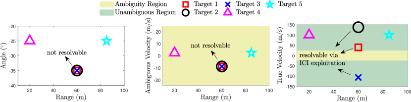
Figure 3: Scenario with multiple targets, illustrated in range-angle, range-ambiguous velocity and range-(true) velocity domains, where target SNRs are given by $\{20,15,10,10,-10\}\,\rm{dB}$, respectively.

Fig. 4 shows the MUSIC spatial spectrum in (19) obtained at the output of Step 1, along with the results of ordinary beamforming. As expected, contrary to ordinary beamforming, MUSIC can correctly identify the different target angles with small number of RX antennas, which is crucial for angle-constrained beamforming in Step 2. In Fig. 5, for each estimated angle $\theta$ in Step 1, we plot the evolution of a normalized version of the GLRT metric in (49), given by

$$0\leq 1-\frac{\mathbf{a}_{\rm{R}}^{H}(\theta)(\mathbf{R}^{*})^{-1}\mathbf{a}_{\rm{R}}(\theta)}{\mathbf{a}_{\rm{R}}^{H}(\theta)\mathbf{Q}^{*}(\nu)^{-1}\mathbf{a}_{\rm{R}}(\theta)}\leq 1\leavevmode\nobreak\ ,$$ (85)

with respect to CFO ($\nu$) through successive iterations of the OMP based interference cancellation algorithm in Algorithm 2 (which corresponds to Step 2 of Algorithm 1). For threshold setting in (85), we use a heuristic value of $0.3$ to declare detection. At iteration $0$, the strongest target at $\theta=-35^{\circ}$, Target 1 with ${\rm{SNR}}=20\,\rm{dB}$, is detected at the peak of the CFO spectrum in (85). Then, at iteration 1, we can observe the effect of cancelling the interference from Target 1 as a valley in the CFO spectrum centered around the velocity of Target 1. In compliance with the scenario in Fig. 3, the second strongest target at $\theta=-35^{\circ}$, Target 2 with ${\rm{SNR}}=15\,\rm{dB}$, yields the largest value in the CFO spectrum at iteration 1. It is seen that as the iterations proceed with successive interference cancellation, weaker targets become more pronounced in the CFO spectrum (e.g., Target 3 from iteration 0 to iteration 2), which implies that the proposed OMP based algorithm in Algorithm 2 can successfully eliminate strong target echoes and enable detection of weak targets in the CFO domain. At the final iteration in Fig. 5, the effects of all targets are removed and thus the peak of the CFO spectrum does not exceed the threshold. Similar trends can be observed in Fig. 5, where, for the illuminated angle $\theta=-25^{\circ}$, a single target is detected at $\nu=100\,\rm{m/s}$, corresponding to the combined response of Target 4 and Target 5 in Fig. 3.

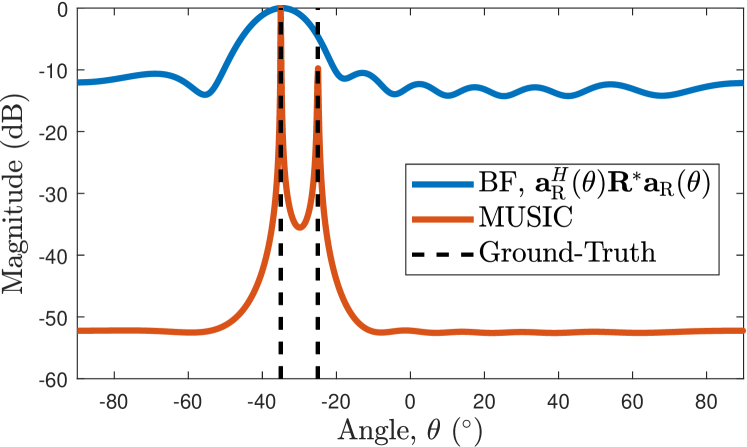
Figure 4: MUSIC spatial spectrum of OFDM radar in Step 1 along with the results of ordinary beamforming (BF) for the scenario in Fig. 3.

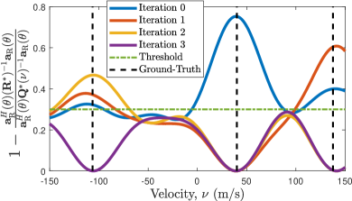
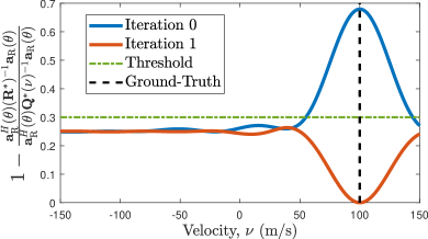
Figure 5: Evolutions of CFO spectrums (i.e., normalized version of the GLRT metric in (49) with respect to CFO $\nu$) obtained for 5 $\theta=-35^{\circ}$ and 5 $\theta=-25^{\circ}$ through successive iterations of interference cancellation based OMP procedure in Algorithm 2 for the scenario in Fig. 3. As the algorithm proceeds through iterations, the effect of interference cancellation manifests itself as valleys in the CFO spectrum corresponding to the velocity of the strongest target in the corresponding iteration.

The results obtained in Step 2 in Fig. 5 reveal one of the core properties of the proposed ICI-aware sensing algorithm: the multi-target ICI exploitation capability with arbitrary transmit symbols. Precisely, the proposed algorithm can resolve Target 1, Target 2 and Target 3 in the CFO domain (indicated as true velocity in the rightmost subfigure in Fig. 3) by exploiting the velocity information conveyed by the ICI effect. As seen from Table I, the ICI effect yields an unambiguous velocity that is $N$ times higher than the standard limit (e.g., in [12, 10, 23]) by virtue of $N$ times faster sampling of fast-time domain compared to slow-time domain in (10). Hence, the proposed ICI exploitation approach can distinguish Target 1, Target 2 and Target 3 as separate objects and estimate their true (i.e., unambiguous) velocities. This is only possible through the novel formulation of ICI-aware sensing in Sec. III, where we decouple the problem of estimating $\nu$ in the fast-time phase rotation matrix $\mathbf{D}(\nu)$ from that of estimating $\nu$ in the slow-time steering vector $\mathbf{c}(\nu)$. On the other hand, the standard 2-D FFT based OFDM radar processing approach [10, 23] only uses slow-time phase progressions for Doppler estimation and thus fails to resolve Target 1, Target 2 and Target 3 since they appear as a unique target in range-angle-ambiguous velocity domains, as shown in Fig. 3.

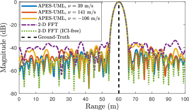
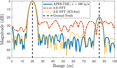
Figure 6: Range profiles obtained for 6 $\theta=-35^{\circ}$ and 6 $\theta=-25^{\circ}$ in Algorithm 3, corresponding to CFOs estimated in Fig. 5, along with the profiles obtained by the FFT benchmarks. When the standard FFT method is employed, the ICI effect leads to masking of Target 5, while APES-UML can successfully eliminate ICI to make the target peak visible as in the ICI-free case.

We now investigate the output of Step 3 of Algorithm 1 (implemented using Algorithm 3), which uses the channel estimates from Step 2 to detect targets in the delay-Doppler domain. Fig. 6 illustrates the range profiles obtained for different angles and CFOs, estimated in Step 1 and Step 2, respectively, along with the range profiles of the FFT based benchmarks. For $\theta=-35^{\circ}$, it is observed that as Target 1, Target 2 and Target 3 lie in the same range bin, their respective range profiles have almost an identical shape. Since these targets are already resolved by the proposed APES-UML algorithm in the CFO domain in the previous step, being co-located in the range domain does not have any effect on their detection performance. For $\theta=-25^{\circ}$, two targets, Target 4 and Target 5, appear at different locations in the range profile of APES-UML corresponding to the CFO, shown in Fig. 5, and the accompanying channel estimate, which is consistent with the scenario in Fig. 3. It is observed from both Fig. 6 and Fig. 6 that the ICI effect leads to increased side-lobe levels for the standard 2-D FFT approach. Meanwhile, the proposed APES-UML algorithm can achieve approximately the same side-lobe levels as the ICI-free case, which proves its multi-target ICI suppression capability (i.e., it can effectively mitigate the ICI effects caused by multiple targets having different velocities via accurate estimation of their CFOs in Step 2). Moreover, we see that ICI-induced high side-lobe levels leads to masking of Target 5 in the range profile of the FFT method, while APES-UML and FFT in the ICI-free case produce a peak at the location of Target 5.

With regard to the implications of Fig. 5 and Fig. 6, it is worth emphasizing another important property of the proposed method: spatial filtering, which is enabled by the MIMO architecture and the APES framework developed in Sec. III-B. By comparing Fig. 5 and Fig. 5, we notice that targets located at different angles do not spill much energy into each other’s CFO spectrum. Similarly, inspecting Fig. 6 and Fig. 6, no leakage can be observed between the range profiles corresponding to different angles. We accomplish this by designing the APES-like cost function in (24), or equivalently, in (50), to perform joint optimization of beamformer, CFO and radar channel, which helps suppress energy leakage outside the desired angle. Therefore, the proposed APES-UML approach can separate out individual target reflections in the angular domain from the mixed signal in (10) by leveraging the multiple-antenna structure.

V-B Detection and Estimation Performance

In this part, we study the detection and estimation performance of the considered OFDM sensing algorithms using $100$ independent Monte Carlo noise realizations. We consider a scenario with two targets as described in Table II, where Target 2 is chosen as the reference target to evaluate performance metrics. The aim is to investigate the masking effect of ICI (due to increased side-lobe levels) under a wide variety of operating conditions, including various SNRs of Target 2 (${\rm{SNR}}\,\rm{dB}$) and target velocities of both targets ($\nu\,\rm{m/s}$) in the presence of a strong target, Target 1.

Table II: Scenario with Varying SNR and Target Velocities

	Range	Velocity	Angle	SNR
Target 1	$40\,\rm{m}$	$\nu\,\rm{m/s}$	$-35^{\circ}$	$25\,\rm{dB}$
Target 2 (Reference)	$80\,\rm{m}$	$\nu\,\rm{m/s}$	$-25^{\circ}$	${\rm{SNR}}\,\rm{dB}$

Fig. 7 shows the probability of detection of the reference target as a function of SNR for three different target velocities. In agreement with the side-lobe performances in Fig. 6, APES-UML significantly outperforms the standard FFT scheme and performs very close to the FFT benchmark that uses ICI-free observations, which proves that the proposed approach can effectively suppress the ICI effect associated with multiple targets. In addition, the detection performance of APES-UML is resilient to target velocity; it can attain the upper bound achievable through ICI-free observations at all target velocities. On the other hand, the performance of 2-D FFT deteriorates as the velocity increases since the ICI effect becomes more severe at higher velocities. At $\nu=120\,\rm{m/s}$, an OFDM radar employing standard 2-D FFT processing [10, 23] becomes completely blind within the SNR range of interest, which clearly indicates the significance of ICI-aware sensing in high-mobility scenarios.

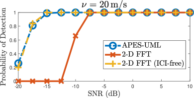
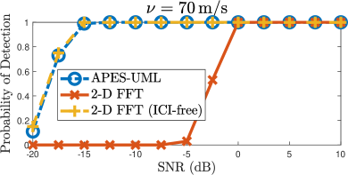
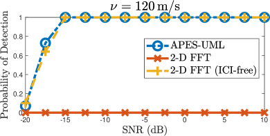
Figure 7: Probability of detection of the reference target with respect to SNR for 7 $\nu=20\,\rm{m/s}$, 7 $\nu=70\,\rm{m/s}$, and 7 $\nu=120\,\rm{m/s}$ for the scenario in Table II.

In Fig. 8, we examine false discovery rates (FDRs), defined as [39] ${\rm{FDR}}={V}/{(V+S)}$, where $V$ is the total number of false alarms (i.e., detections that cannot be associated to the existing targets) and $S$ is the total number of reference target detections over all Monte Carlo runs. Similar to the probability of detection curves, APES-UML exhibits a false alarm performance that is very close to FFT with ICI-free observations, which proves the multi-target ICI compensation capability of the proposed approach. From Fig. 7 and Fig. 8, we conclude that, except for the case of high SNR and low-mobility, the standard FFT method fails.

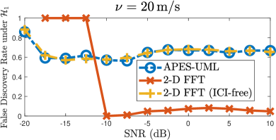
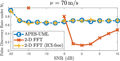
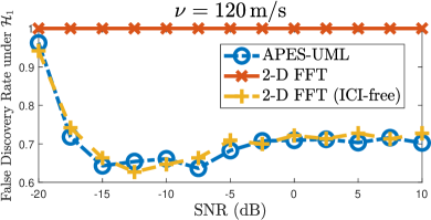
Figure 8: False discovery rate under $\mathcal{H}_{1}$ with respect to SNR for 8 $\nu=20\,\rm{m/s}$, 8 $\nu=70\,\rm{m/s}$, and 8 $\nu=120\,\rm{m/s}$ for the scenario in Table II. No values are shown if there is neither a detection nor a false alarm.

We now turn our attention to estimation performances of the considered schemes. Fig. 9 shows the root mean-squared errors (RMSEs) of range estimation of the reference target as a function of SNR for various target velocities. The RMSE is calculated as [40]

$${\rm{RMSE}}=\left(\mathbb{E}\Big{\{}(\widehat{R}-R)^{2}\leavevmode\nobreak\ \lvert\leavevmode\nobreak\ {\rm{target\leavevmode\nobreak\ detected}}\Big{\}}\right)^{1/2}\leavevmode\nobreak\ ,$$ (89)

where $\widehat{R}$ and $R$ denote, respectively, the estimated and true range values. As expected, the 2-D FFT benchmark cannot estimate target parameters below a certain SNR threshold (depending on velocity) due to lack of detections, in compliance with Fig. 7. In addition, the proposed APES-UML algorithm achieves almost the same range RMSE performance as the ICI-free benchmark, which again evidences its superior ICI elimination capability. Moreover, APES-UML exhibits consistent range estimation performance at all target velocities; no noticeable changes can be observed in the range RMSE of APES-UML with increasing velocity, whereas the ICI effect significantly degrades the performance of FFT method, especially at high velocities.

In Fig. 10, we plot the velocity RMSEs of the reference target with respect to SNR, calculated similarly to (89). For $\nu=20\,\rm{m/s}$, similar trends to the case of range RMSE can be observed. However, for $\nu=70\,\rm{m/s}$ and $\nu=120\,\rm{m/s}$, both of the FFT-based methods fail to correctly estimate velocity since the unambiguous velocity is $v_{\rm{max}}=\pm 24.41\,\rm{m/s}$, as seen from Table I. Through simultaneous mitigation (via joint CFO/channel estimation in Algorithm 2) and exploitation (by resolving velocity ambiguity in Algorithm 3) of ICI, APES-UML can estimate the true velocity of the target with high accuracy. Hence, the proposed approach can even outperform the ICI-free benchmark in such scenarios by turning ICI from foe to friend.

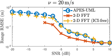
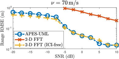
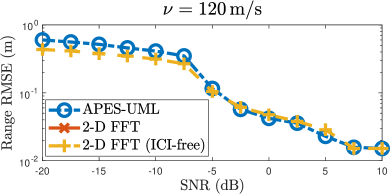
Figure 9: Range RMSE of the reference target with respect to SNR for 9 $\nu=20\,\rm{m/s}$, 9 $\nu=70\,\rm{m/s}$, and 9 $\nu=120\,\rm{m/s}$ for the scenario in Table II.

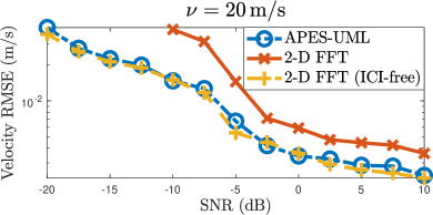
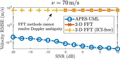
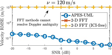
Figure 10: Velocity RMSE of the reference target with respect to SNR for 10 $\nu=20\,\rm{m/s}$, 10 $\nu=70\,\rm{m/s}$, and 10 $\nu=120\,\rm{m/s}$ for the scenario in Table II.

VI Concluding Remarks

We have addressed the multi-target detection/estimation problem for a MIMO-OFDM DFRC system in the presence of non-negligible ICI caused by high-mobility targets. By formulating the ICI-aware sensing as a joint CFO/channel estimation problem, we have developed a novel three-step algorithm for multiple target detection and delay-Doppler-angle estimation. Remarkably, the proposed algorithm can mitigate the ICI effect induced by multiple targets having different radial velocities, which prevents degradation in detection/estimation performance, and at the same time exploit ICI to resolve Doppler ambiguity of the detected targets. Extensive simulation results have shown that the proposed approach significantly outperforms the traditional FFT based method and can attain the performance achievable in the absence of ICI, with respect to various metrics such as probability of detection and range/velocity estimation accuracy. This indicates that ICI can be successfully suppressed in multi-target scenarios with arbitrary OFDM data symbols, which is crucial for high-speed vehicular JRC applications.

Supplementary Material For Is ICI Friend or Foe? Musa Furkan Keskin, Henk Wymeersch, Visa Koivunen

VII Spatial Covariance Matrix of OFDM Radar Observations in (15)

In this part, we derive the SCM of the radar data cube in (15). Plugging (14) into (15) yields

$$\mathbf{R} =\sum_{k_{1}=0}^{K-1}\sum_{k_{2}=0}^{K-1}\Bigg{[}\alpha_{k_{1}}^{*}\alpha_{k_{2}}\,\mathbf{a}_{\rm{T}}^{H}(\theta_{k_{1}})\mathbf{f}_{\rm{T}}^{*}\,\mathbf{a}_{\rm{T}}^{T}(\theta_{k_{2}})\mathbf{f}_{\rm{T}}\,\mathbf{a}_{\rm{R}}^{*}(\theta_{k_{1}})\,\mathbf{a}_{\rm{R}}^{T}(\theta_{k_{2}})$$

$$\leavevmode\nobreak\ \leavevmode\nobreak\ \times\mathbf{b}^{H}(\tau_{k_{1}})\Bigg{(}\sum_{m=0}^{M-1}\left[\mathbf{c}(\nu_{k_{1}})\right]_{m}\left[\mathbf{c}^{*}(\nu_{k_{2}})\right]_{m}{\rm{diag}}\left(\mathbf{x}_{m}\right)^{H}$$

$$\leavevmode\nobreak\ \leavevmode\nobreak\ \leavevmode\nobreak\ \leavevmode\nobreak\ \times\mathbf{F}_{N}\mathbf{D}^{H}(\nu_{k_{1}})\mathbf{D}(\nu_{k_{2}})\mathbf{F}_{N}^{H}{\rm{diag}}\left(\mathbf{x}_{m}\right)\Bigg{)}\mathbf{b}(\tau_{k_{2}})\Bigg{]}$$

$$\leavevmode\nobreak\ \leavevmode\nobreak\ +NM\sigma^{2}{\bm{\mathrm{I}}}\leavevmode\nobreak\ ,$$ (90)

where we invoke the law of large numbers to approximate the noise covariance as

$$\sum_{m=0}^{M-1}\macc@depth\char 1\relax\frozen@everymath{\macc@group}\macc@set@skewchar\macc@nested@a 111{\mathbf{Z}}_{m}^{H}\macc@depth\char 1\relax\frozen@everymath{\macc@group}\macc@set@skewchar\macc@nested@a 111{\mathbf{Z}}_{m}\approx\mathbb{E}\left\{\sum_{m=0}^{M-1}\macc@depth\char 1\relax\frozen@everymath{\macc@group}\macc@set@skewchar\macc@nested@a 111{\mathbf{Z}}_{m}^{H}\macc@depth\char 1\relax\frozen@everymath{\macc@group}\macc@set@skewchar\macc@nested@a 111{\mathbf{Z}}_{m}\right\}=NM\sigma^{2}{\bm{\mathrm{I}}}\leavevmode\nobreak\ ,$$ (91)

provided that $M$ and/or $N$ is sufficiently large. Similarly, to ignore signal-noise cross terms in (90), the law of large numbers is employed based on the fact that transmit data symbols and noise are uncorrelated.

Using (8) and the unitary property of the DFT matrix, we can write the direct and cross-target terms separately in (90):

$$\mathbf{R} =\mathbf{R}^{\rm{direct}}+\mathbf{R}^{\rm{cross}}+NM\sigma^{2}{\bm{\mathrm{I}}}\leavevmode\nobreak\ ,$$ (92)

where

$$\mathbf{R}^{\rm{direct}} =\sum_{k=0}^{K-1}\Bigg{[}\lvert\alpha_{k}\rvert^{2}\,\lvert\mathbf{a}_{\rm{T}}^{T}(\theta_{k})\mathbf{f}_{\rm{T}}\rvert^{2}\,\mathbf{a}_{\rm{R}}^{*}(\theta_{k})\mathbf{a}_{\rm{R}}^{T}(\theta_{k})$$ (93)

$$\times\mathbf{b}^{H}(\tau_{k}) \left(\sum_{m=0}^{M-1}\Big{\lvert}\left[\mathbf{c}(\nu_{k})\right]_{m}\Big{\rvert}^{2}{\rm{diag}}\left(\mathbf{x}_{m}\right)^{H}{\rm{diag}}\left(\mathbf{x}_{m}\right)\right)\mathbf{b}(\tau_{k})\Bigg{]}\leavevmode\nobreak\ ,$$

$$\mathbf{R}^{\rm{cross}}$$ (94)

$$=\sum_{k_{1}=0}^{K-1}\sum_{\begin{subarray}{c}k_{2}=0\\ k_{2}\neq k_{1}\end{subarray}}^{K-1}\Bigg{[}\alpha_{k_{1}}^{*}\alpha_{k_{2}}\,\mathbf{a}_{\rm{T}}^{H}(\theta_{k_{1}})\mathbf{f}_{\rm{T}}^{*}\,\mathbf{a}_{\rm{T}}^{T}(\theta_{k_{2}})\mathbf{f}_{\rm{T}}\,\mathbf{a}_{\rm{R}}^{*}(\theta_{k_{1}})\,\mathbf{a}_{\rm{R}}^{T}(\theta_{k_{2}})$$

$$\leavevmode\nobreak\ \leavevmode\nobreak\ \times\mathbf{b}^{H}(\tau_{k_{1}})\Bigg{(}\sum_{m=0}^{M-1}\left[\mathbf{c}(\nu_{k_{1}})\right]_{m}\left[\mathbf{c}^{*}(\nu_{k_{2}})\right]_{m}{\rm{diag}}\left(\mathbf{x}_{m}\right)^{H}$$

$$\leavevmode\nobreak\ \leavevmode\nobreak\ \leavevmode\nobreak\ \leavevmode\nobreak\ \times\mathbf{F}_{N}\mathbf{D}(\nu_{k_{2}}-\nu_{k_{1}})\mathbf{F}_{N}^{H}{\rm{diag}}\left(\mathbf{x}_{m}\right)\Bigg{)}\mathbf{b}(\tau_{k_{2}})\Bigg{]}\leavevmode\nobreak\ .$$

Using (13) and the unit-magnitude property of the steering vector elements in (6) and (7), the direct term in (93) becomes

$$\mathbf{R}^{\rm{direct}} =\left\lVert\mathbf{X}\right\rVert_{F}^{2}\sum_{k=0}^{K-1}\lvert\alpha_{k}\rvert^{2}\lvert\mathbf{a}_{\rm{T}}^{T}(\theta_{k})\mathbf{f}_{\rm{T}}\rvert^{2}\mathbf{a}_{\rm{R}}^{*}(\theta_{k})\mathbf{a}_{\rm{R}}^{T}(\theta_{k})\leavevmode\nobreak\ .$$ (95)

Applying the law of large numbers and utilizing the covariance of $\mathbf{X}$ in (16), we can approximate (95) as

$$\mathbf{R}^{\rm{direct}} \approx NM\sigma_{x}^{2}\sum_{k=0}^{K-1}\lvert\alpha_{k}\rvert^{2}\lvert\mathbf{a}_{\rm{T}}^{T}(\theta_{k})\mathbf{f}_{\rm{T}}\rvert^{2}\mathbf{a}_{\rm{R}}^{*}(\theta_{k})\mathbf{a}_{\rm{R}}^{T}(\theta_{k})\leavevmode\nobreak\ .$$ (96)

With regard to the cross-term in (94), using the properties of the Hadamard product, we can write

$$\mathbf{A}_{m} \triangleq{\rm{diag}}\left(\mathbf{x}_{m}\right)^{H}\mathbf{F}_{N}\mathbf{D}(\nu_{k_{2}}-\nu_{k_{1}})\mathbf{F}_{N}^{H}{\rm{diag}}\left(\mathbf{x}_{m}\right)$$ (97)

$$=\left(\mathbf{x}_{m}\mathbf{x}_{m}^{H}\right)^{*}\odot\mathbf{F}_{N}\mathbf{D}(\nu_{k_{2}}-\nu_{k_{1}})\mathbf{F}_{N}^{H}\leavevmode\nobreak\ .$$

Assuming sufficiently large $M$, we invoke the law of large numbers to obtain

$$\sum_{m=0}^{M-1}\left[\mathbf{c}(\nu_{k_{1}})\right]_{m}\left[\mathbf{c}^{*}(\nu_{k_{2}})\right]_{m}\mathbf{A}_{m}$$ (98)

$$\leavevmode\nobreak\ \leavevmode\nobreak\ \leavevmode\nobreak\ \leavevmode\nobreak\ \approx\sum_{m=0}^{M-1}\left[\mathbf{c}(\nu_{k_{1}})\right]_{m}\left[\mathbf{c}^{*}(\nu_{k_{2}})\right]_{m}\mathbb{E}\{\mathbf{A}_{m}\}\leavevmode\nobreak\ ,$$

where expectation is over the distribution of data symbols $\mathbf{x}_{m}$. Based on (97) and using the covariance of data symbols in (16), we have

$$\mathbb{E}\{\mathbf{A}_{m}\} =\mathbb{E}\left\{\left(\mathbf{x}_{m}\mathbf{x}_{m}^{H}\right)^{*}\right\}\odot\mathbf{F}_{N}\mathbf{D}(\nu_{k_{2}}-\nu_{k_{1}})\mathbf{F}_{N}^{H}$$ (99)

$$=\sigma_{x}^{2}{\bm{\mathrm{I}}}\odot\mathbf{F}_{N}\mathbf{D}(\nu_{k_{2}}-\nu_{k_{1}})\mathbf{F}_{N}^{H}$$

$$=\sigma_{x}^{2}{\bm{\mathrm{I}}}\odot\sum_{n=0}^{N-1}d_{n}\mathbf{f}_{n}\mathbf{f}_{n}^{H}$$

$$=\underbrace{\left(\sigma_{x}^{2}+\sum_{n=0}^{N-1}d_{n}\right)}_{\triangleq\gamma}{\bm{\mathrm{I}}}\leavevmode\nobreak\ ,$$

where

$$\mathbf{F}_{N} \triangleq\left[\mathbf{f}_{0}\leavevmode\nobreak\ \ldots\leavevmode\nobreak\ \mathbf{f}_{N-1}\right]\leavevmode\nobreak\ ,$$ (100)

$$d_{n} \triangleq\left[\mathbf{D}(\nu_{k_{2}}-\nu_{k_{1}})\right]_{n,n}\leavevmode\nobreak\ .$$ (101)

Inserting (99) and (98) into (94) yields

$$\mathbf{R}^{\rm{cross}}$$ (102)

$$\approx\gamma\sum_{k_{1}=0}^{K-1}\sum_{\begin{subarray}{c}k_{2}=0\\ k_{2}\neq k_{1}\end{subarray}}^{K-1}\Bigg{[}\alpha_{k_{1}}^{*}\alpha_{k_{2}}\,\mathbf{a}_{\rm{T}}^{H}(\theta_{k_{1}})\mathbf{f}_{\rm{T}}^{*}\,\mathbf{a}_{\rm{T}}^{T}(\theta_{k_{2}})\mathbf{f}_{\rm{T}}\,\mathbf{a}_{\rm{R}}^{*}(\theta_{k_{1}})\,\mathbf{a}_{\rm{R}}^{T}(\theta_{k_{2}})$$

$$\leavevmode\nobreak\ \leavevmode\nobreak\ \leavevmode\nobreak\ \leavevmode\nobreak\ \leavevmode\nobreak\ \leavevmode\nobreak\ \times\mathbf{b}^{H}(\tau_{k_{1}})\mathbf{b}(\tau_{k_{2}})\mathbf{c}^{H}(\nu_{k_{2}})\mathbf{c}(\nu_{k_{1}})\Bigg{]}\leavevmode\nobreak\ .$$

Under the assumption in (17), the cross-term in (102) disappears, i.e.,

$$\mathbf{R}^{\rm{cross}}\approx{{\bm{0}}}_{N_{\rm{R}}\times N_{\rm{R}}}\leavevmode\nobreak\ .$$ (103)

Finally, we insert (96) and (103) into (92) to obtain

$$\mathbf{R} =NM\sigma_{x}^{2}\sum_{k=0}^{K-1}\lvert\alpha_{k}\rvert^{2}\lvert\mathbf{a}_{\rm{T}}^{T}(\theta_{k})\mathbf{f}_{\rm{T}}\rvert^{2}\mathbf{a}_{\rm{R}}^{*}(\theta_{k})\mathbf{a}_{\rm{R}}^{T}(\theta_{k})+NM\sigma^{2}{\bm{\mathrm{I}}}\leavevmode\nobreak\ ,$$

which completes the proof.

References

- [1] Musa Furkan Keskin, Henk Wymeersch, and Visa Koivunen, “ICI-aware parameter estimation for MIMO-OFDM radar via APES spatial filtering,” in 2021 IEEE International Conference on Acoustics, Speech and Signal Processing (ICASSP), accepted for publication.
- [2] F. Liu, C. Masouros, A. Petropulu, H. Griffiths, and L. Hanzo, “Joint radar and communication design: Applications, state-of-the-art, and the road ahead,” IEEE Transactions on Communications, pp. 1–1, 2020.
- [3] K. V. Mishra, M. R. Bhavani Shankar, V. Koivunen, B. Ottersten, and S. A. Vorobyov, “Toward millimeter-wave joint radar communications: A signal processing perspective,” IEEE Signal Processing Magazine, vol. 36, no. 5, pp. 100–114, Sep. 2019.
- [4] L. Zheng, M. Lops, Y. C. Eldar, and X. Wang, “Radar and communication coexistence: An overview: A review of recent methods,” IEEE Signal Processing Magazine, vol. 36, no. 5, pp. 85–99, 2019.
- [5] Alex R Chiriyath, Bryan Paul, and Daniel W Bliss, “Radar-communications convergence: Coexistence, cooperation, and co-design,” IEEE Transactions on Cognitive Communications and Networking, vol. 3, no. 1, pp. 1–12, 2017.
- [6] Dingyou Ma, Nir Shlezinger, Tianyao Huang, Yimin Liu, and Yonina C Eldar, “Joint radar-communication strategies for autonomous vehicles: Combining two key automotive technologies,” IEEE Signal Processing Magazine, vol. 37, no. 4, pp. 85–97, 2020.
- [7] C. Aydogdu, M. F. Keskin, G. K. Carvajal, O. Eriksson, H. Hellsten, H. Herbertsson, E. Nilsson, M. Rydstrom, K. Vanas, and H. Wymeersch, “Radar interference mitigation for automated driving: Exploring proactive strategies,” IEEE Signal Processing Magazine, vol. 37, no. 4, pp. 72–84, 2020.
- [8] A. Hassanien, M. G. Amin, E. Aboutanios, and B. Himed, “Dual-function radar communication systems: A solution to the spectrum congestion problem,” IEEE Signal Processing Magazine, vol. 36, no. 5, pp. 115–126, Sep. 2019.
- [9] F. Liu, L. Zhou, C. Masouros, A. Li, W. Luo, and A. Petropulu, “Toward dual-functional radar-communication systems: Optimal waveform design,” IEEE Transactions on Signal Processing, vol. 66, no. 16, pp. 4264–4279, Aug 2018.
- [10] C. Sturm and W. Wiesbeck, “Waveform design and signal processing aspects for fusion of wireless communications and radar sensing,” Proceedings of the IEEE, vol. 99, no. 7, pp. 1236–1259, July 2011.
- [11] M. Bică and V. Koivunen, “Generalized multicarrier radar: Models and performance,” IEEE Transactions on Signal Processing, vol. 64, no. 17, pp. 4389–4402, Sep. 2016.
- [12] Fuqiang Zhang, Zenghui Zhang, Wenxian Yu, and Trieu-Kien Truong, “Joint range and velocity estimation with intrapulse and intersubcarrier Doppler effects for OFDM-based RadCom systems,” IEEE Transactions on Signal Processing, vol. 68, pp. 662–675, 2020.
- [13] R. F. Tigrek, W. J. A. De Heij, and P. Van Genderen, “OFDM signals as the radar waveform to solve Doppler ambiguity,” IEEE Transactions on Aerospace and Electronic Systems, vol. 48, no. 1, pp. 130–143, Jan 2012.
- [14] Sayed Hossein Dokhanchi, Bhavani Shankar Mysore, Kumar Vijay Mishra, and Björn Ottersten, “A mmWave automotive joint radar-communications system,” IEEE Transactions on Aerospace and Electronic Systems, vol. 55, no. 3, pp. 1241–1260, 2019.
- [15] G. Hakobyan, M. Ulrich, and B. Yang, “OFDM-MIMO radar with optimized nonequidistant subcarrier interleaving,” IEEE Transactions on Aerospace and Electronic Systems, vol. 56, no. 1, pp. 572–584, 2020.
- [16] Gor Hakobyan and Bin Yang, “A novel intercarrier-interference free signal processing scheme for OFDM radar,” IEEE Transactions on Vehicular Technology, vol. 67, no. 6, pp. 5158–5167, 2017.
- [17] Jinsoo Lim, Sung-Rae Kim, and Dong-Joon Shin, “Two-step Doppler estimation based on intercarrier interference mitigation for OFDM radar,” IEEE Antennas and Wireless Propagation Letters, vol. 14, pp. 1726–1729, 2015.
- [18] Yinghao Ge, Weile Zhang, Feifei Gao, and Hlaing Minn, “Angle-domain approach for parameter estimation in high-mobility OFDM with fully/partly calibrated massive ULA,” IEEE Transactions on Wireless Communications, vol. 18, no. 1, pp. 591–607, 2018.
- [19] Xuanxuan Tian, Tingting Zhang, Qinyu Zhang, and Zhaohui Song, “High accuracy Doppler processing with low complexity in OFDM-based RadCom systems,” IEEE Communications Letters, vol. 21, no. 12, pp. 2618–2621, 2017.
- [20] Gabriel Lellouch, Amit Mishra, and Michael Inggs, “Impact of the Doppler modulation on the range and Doppler processing in OFDM radar,” in 2014 IEEE Radar Conference. IEEE, 2014, pp. 0803–0808.
- [21] Qing Zhou, Xuanxuan Tian, and Tingting Zhang, “Low complexity ICI mitigation in OFDM based RadCom systems,” in 2020 International Conference on Wireless Communications and Signal Processing (WCSP). IEEE, 2020, pp. 1022–1027.
- [22] Luzhou Xu, Jian Li, and Petre Stoica, “Target detection and parameter estimation for MIMO radar systems,” IEEE Transactions on Aerospace and Electronic Systems, vol. 44, no. 3, pp. 927–939, 2008.
- [23] Martin Braun, “OFDM radar algorithms in mobile communication networks,” Ph. D. dissertation, 2014.
- [24] Weile Zhang, Qinye Yin, and Wenjie Wang, “Blind closed-form carrier frequency offset estimation for OFDM with multi-antenna receiver,” IEEE Transactions on Vehicular Technology, vol. 64, no. 8, pp. 3850–3856, 2014.
- [25] Ralph Schmidt, “Multiple emitter location and signal parameter estimation,” IEEE transactions on antennas and propagation, vol. 34, no. 3, pp. 276–280, 1986.
- [26] K. Luo and A. Manikas, “Superresolution multitarget parameter estimation in MIMO radar,” IEEE Transactions on Geoscience and Remote Sensing, vol. 51, no. 6, pp. 3683–3693, 2013.
- [27] Y. L. Sit, B. Nuss, and T. Zwick, “On mutual interference cancellation in a MIMO OFDM multiuser radar-communication network,” IEEE Transactions on Vehicular Technology, vol. 67, no. 4, pp. 3339–3348, April 2018.
- [28] Martin Braun, “OFDM radar algorithms in mobile communication networks,” Karlsruher Institutes für Technologie, 2014.
- [29] P. Kumari, J. Choi, N. González-Prelcic, and R. W. Heath, “IEEE 802.11ad-based radar: An approach to joint vehicular communication-radar system,” IEEE Transactions on Vehicular Technology, vol. 67, no. 4, pp. 3012–3027, April 2018.
- [30] P. Kumari, S. A. Vorobyov, and R. W. Heath, “Adaptive virtual waveform design for millimeter-wave joint communication–radar,” IEEE Transactions on Signal Processing, vol. 68, pp. 715–730, 2020.
- [31] Y. . Liang, R. Schober, and W. Gerstacker, “Time-domain transmit beamforming for MIMO-OFDM systems with finite rate feedback,” IEEE Transactions on Communications, vol. 57, no. 9, pp. 2828–2838, 2009.
- [32] Timo Roman, Samuli Visuri, and Visa Koivunen, “Blind frequency synchronization in OFDM via diagonality criterion,” IEEE Transactions on Signal Processing, vol. 54, no. 8, pp. 3125–3135, 2006.
- [33] Y. Ge, W. Zhang, F. Gao, and G. Y. Li, “Frequency synchronization for uplink massive MIMO with adaptive MUI suppression in angle domain,” IEEE Transactions on Signal Processing, vol. 67, no. 8, pp. 2143–2158, 2019.
- [34] A Lee Swindlehurst, “Time delay and spatial signature estimation using known asynchronous signals,” IEEE Transactions on Signal Processing, vol. 46, no. 2, pp. 449–462, 1998.
- [35] Alessio Fascista, Angelo Coluccia, Henk Wymeersch, and Gonzalo Seco-Granados, “Millimeter-wave downlink positioning with a single-antenna receiver,” IEEE Transactions on Wireless Communications, vol. 18, no. 9, pp. 4479–4490, 2019.
- [36] Jack Capon, “High-resolution frequency-wavenumber spectrum analysis,” Proceedings of the IEEE, vol. 57, no. 8, pp. 1408–1418, 1969.
- [37] Stéphane G Mallat and Zhifeng Zhang, “Matching pursuits with time-frequency dictionaries,” IEEE Transactions on signal processing, vol. 41, no. 12, pp. 3397–3415, 1993.
- [38] Mark A Richards, Fundamentals of Radar Signal Processing, Tata McGraw-Hill Education, 2005.
- [39] Priyadip Ray and Pramod K Varshney, “Radar target detection framework based on false discovery rate,” IEEE Transactions on Aerospace and Electronic Systems, vol. 47, no. 2, pp. 1277–1292, 2011.
- [40] Emanuele Grossi, Marco Lops, and Luca Venturino, “Adaptive detection and localization exploiting the IEEE 802.11 ad standard,” IEEE Transactions on Wireless Communications, 2020.