Martingale posterior distributions
Abstract
The prior distribution on parameters of a sampling distribution is the usual starting point for Bayesian uncertainty quantification. In this paper, we present a different perspective which focuses on missing observations as the source of statistical uncertainty, with the parameter of interest being known precisely given the entire population. We argue that the foundation of Bayesian inference is to assign a distribution on missing observations conditional on what has been observed. In the conditionally i.i.d. setting with an observed sample of size , the Bayesian would thus assign a predictive distribution on the missing conditional on , which then induces a distribution on the parameter.
Demonstrating an application of martingales, Doob shows that choosing the Bayesian predictive distribution returns the conventional posterior as the distribution of the parameter. Taking this as our cue, we relax the predictive machine, avoiding the need for the predictive to be derived solely from the usual prior to posterior to predictive density formula. We introduce the martingale posterior distribution, which returns Bayesian uncertainty directly on any statistic of interest without the need for the likelihood and prior, and this distribution can be sampled through a computational scheme we name predictive resampling. To that end, we introduce new predictive methodologies for multivariate density estimation, regression and classification that build upon recent work on bivariate copulas.
Keywords: Bayesian uncertainty; Copula; Martingale; Predictive inference
1 Introduction
Statistical uncertainty in a parameter of interest arises due to missing observations. If a complete population is observed, then the parameter of interest can be assumed to be known precisely. In this paper, we argue that the Bayesian accounts for this uncertainty by constructing a distribution on the missing observations conditional on what has been observed. This in turn induces a distribution on the parameter given the observed data, which we will see is the posterior distribution. In this work, we will describe and generalize this framework in detail for the case where the observations are independent and identically distributed (i.i.d.), and we will also briefly consider other data structures.
In the conditionally i.i.d. case, given where is the unknown true sampling distribution, the missing observations are the remaining , and as such we focus our modelling efforts directly on the predictive density
| (1.1) |
Here, the construction of the predictive density is for parameter inference, and not for forecasting future observations as is more usual. For inference, we assume that the object of interest is fully defined once all the observations have been viewed, which we write as . It is clear then that (1.1) induces a distribution on , and we call this scheme of imputing and computing as predictive resampling. A key observation is that will always contain the observed as the predictive Bayesian considers the observed sample to be fixed, in contrast to the frequentist consideration of other possible values of .
For conditionally i.i.d. observations, the traditional Bayesian approach is to elicit a prior density and likelihood function , derive the posterior , then compute the predictive density through
| (1.2) |
A concise summary of our approach is the following: while de Finetti, (1937) provided a representation of Bayesian inference which relies on exchangeability and the prior distribution, Doob, (1949) provided a framework which relies solely, in the i.i.d. case, on the predictive distribution. We will see that Doob’s framework is more flexible and the mathematical requirement amounts to the construction of a martingale. It is this flexibility provided by Doob’s framework which we exploit in this paper. In fact, through Doob’s theorem, we will see that predictive resampling as described above is identical to posterior sampling when using (1.2) as the predictive and indexes the sampling density, in which case . Denoting as the prior predictive, this connection is illustrated below for the traditional Bayesian case:
However, the traditional Bayesian focus on the prior on makes no appeal to the underlying cause of the uncertainty, that is the unobserved part of the study population . Furthermore, the traditional prior to posterior computation is becoming increasingly strained as model complexity and data sizes grow. In our work, we advocate the predictive resampling strategy - given , our starting point is directly the predictive model (1.1) and the target statistic of interest , noting now that is no longer restricted to indexing the sampling density. We relax de Finetti’s assumption of exchangeability, but we must now take care to construct (1.1) so that is indeed convergent to some , where can be viewed as an estimator. We highlight here that we use and for the size of the observed dataset and the imputed population respectively. In the spirit of Doob, we rely heavily on martingales, which also aid in ensuring that expectations of limits coincide with fixed quantities seen at the sample of size . This can be regarded as a predictive coherency condition, and we designate the distribution of as the martingale posterior. Our choice of (1.1) will be density estimators based on recent ideas in the literature, specifically the conditionally identically distributed (c.i.d.) sequence of Berti et al., (2004) and bivariate copula update of Hahn et al., (2018).
We now discuss why one would want to go through the route of obtaining the martingale posterior via the induced distribution of from (1.1) rather than the traditional likelihood-prior construction. Firstly, predictive models are probabilistic statements on observables, which removes the need to elicit subjective probability distributions on parameters which may have no real-world interpretations and only index the sampling density. Secondly, the martingale posterior establishes a direct connection between prediction and statistical inference, opening up the possibility of using modern probabilistic predictive methods for inference (Breiman,, 2001), and transparently acknowledges the source of statistical uncertainty as the missing . Thirdly, working directly with predictive distributions is highly practical. For an elicited 1-step ahead predictive, we can predictively resample by carrying out the recursive update
to sample for a large enough such that has effectively converged to a sample from the martingale posterior, or matches a known finite study population size. In complex scenarios such as multivariate density estimation and regression, we introduce new copula-based methodologies where our computations remain exact, GPU-friendly and parallelizable, returning us Bayesian uncertainty without any reliance on Markov chain Monte Carlo (MCMC). Finally, a predictive approach more clearly delineates the core similarities and differences between Bayesian and frequentist uncertainty.
We will focus on the conditionally i.i.d. data setting in this work, which corresponds to exchangeable traditional Bayesian models. In this setting, the martingale posterior can indeed be regarded as a generalization of the traditional Bayesian model, as the class of c.i.d. models is more general and contains the class of exchangeable models which we will see in Section 3.2. In more complex data structures beyond i.i.d. data, such as those encountered in hierarchical modelling or time series, our framework would still apply. In this case, the missing observations we require may no longer be , and model elicitation would no longer only involve a sequence of predictive distributions. For example, a simple hierarchical setting is the observation process , where is itself drawn from an unknown and we may be interested in some functional . Here, we only observe , so the missing observations of interest are now the unobserved random effects . We can thus seek to impute from the data, followed by the missing remainder . Computing would then return us a posterior sample. For the remainder of the paper, we will focus only on the i.i.d. case and leave the details of non-i.i.d. settings for future work.
In Section 2, we formally investigate the connection between predictive and posterior inference, and introduce a predictive framework for inference and the resulting martingale posterior. We then utilize the bootstrap as a canonical example to distinctly compare Bayesian and frequentist uncertainty. We postpone discussion of related work until Section 2.5 in order to provide context beforehand. In Section 3, we discuss predictive coherence conditions for martingale posteriors, utilizing c.i.d. sequences. In Section 4, we revisit the bivariate copula methodology of Hahn et al., (2018) for univariate density estimation, and extend it to obtain the martingale posterior. We then generalize this copula-based method to multivariate density estimation, regression and classification. Section 5 then provides a thorough demonstration of the above methods through examples. In Section 6, we discuss some theoretical properties of the martingale posterior with the copula-based methodology. Finally, we discuss our results in Section 7.
2 A predictive framework for inference
2.1 Doob’s theorem and Bayesian uncertainty
Uncertainty quantification lies at the core of statistical inference, and Bayesian inference is one framework for handling uncertainty in a formal manner. The Bayesian begins with the random variables , where are the observables of interest, and is the parameter which indexes the sampling density . We assume throughout that the appropriate densities exist. For conditionally i.i.d. data, the Bayesian elicits a joint probability model for the observables and parameter with joint density
| (2.1) |
for each . Here, the density represents prior knowledge about the parameter which generates the observations, and under a Subjectivist point of view, represents the subjective probability that the generating parameter value lies in the set . Marginalizing out gives the joint density of the observables,
| (2.2) |
De Finetti however argued that the direct likelihood–prior interpretation of the Bayesian model was insufficient, as is of a “metaphysical” nature and probability statements should only be on observables (Bernardo and Smith,, 2009). This then motivated the notion of exchangeability, where the joint probability of the observables is invariant to the ordering of for all . Through de Finetti’s representation theorem (de Finetti,, 1937) and extensions thereof (e.g. Hewitt and Savage, (1955)), the assumption of exchangeability induces the likelihood-prior form of the joint density in (2.2) (where may not have a density), which motivates such a specification of the Bayesian model. The representation theorem however is only part of the story. As alluded to in the Section 1, the source of statistical uncertainty is the lack of the infinite dataset with which we could pin down any quantity of interest precisely. Bayesian uncertainty through the lens of the prior is still opaque in this regard, even with the representation theorem. The key to understanding the source of uncertainty lies in the predictive imputation of observables, for which we require a result from Doob.
Let us assume that data has yet to be observed, so the missing observations are . Following the discussion in Section 1, one can regard (2.2) as the predictive density on the missing population, and can estimate the parameter indexing the sampling density as a function of the imputed . An appropriate and intuitive point estimate for the Bayesian is the posterior mean, which we write as
A secondary result of Doob, (1949) confirms that the prior uncertainty in is equivalent to the predictive uncertainty in .
Theorem 1 (Doob, (1949)).
Assume is in a linear space with , and is distributed according to (2.1), so . Under measurability and identifiability conditions on , we have
| (2.3) |
For the above result, the key is to rely on being a martingale, that is
almost surely. Doob’s martingale convergence theorem then ensures that converges to a limit almost surely. For in more general metric spaces, consistency results with general notions of posterior expectations are provided in Ghosal and van der Vaart, (2017, Theorem 6.8). As an aside, we highlight that Doob, (1949) provides a more general result: the Bayesian posterior distribution converges weakly to the Dirac measure almost surely for -almost every as . The technical details of a more general version of this result can be found in Ghosal and van der Vaart, (2017, Theorem 6.9). In the Bayesian nonparametric case where is a probability density function, we have a nonparametric extension of the above results (Lijoi et al.,, 2004).
Returning to the task at hand, we can summarize the above by considering two distinct methods of sampling from the prior before seeing any data. The first is to draw directly, which is the opaque view of the inherently random parameter that we are trying to shed light on. The second, which inspires the remainder of our paper, begins with sequentially imputing the unseen observables from the sequence of predictive densities
| (2.4) |
until we have the complete information in the limit. Given this random infinite dataset, the limiting point estimate , that is the posterior mean computed on the entire dataset, is in fact distributed according to . This equivalence highlights the fact that a priori uncertainty in and uncertainty in are one and the same, and the function provides a means to precisely recover our quantity of interest when all information is made available to us.
Of course, such an interpretation is equally valid a posteriori, that is after we have observed . Here, sampling is equivalent to sampling conditional on and computing as if we have observed the infinite dataset, noting that is now fixed. This can be seen by simply substituting the prior in (2.1), (2.2) and Theorem 1 with the posterior . In conclusion, Doob’s result highlights that the Bayesian seeks to simulate what is needed to pin down the parameter but is missing from reality, that is in the i.i.d. case, and we find this to be a compelling justification for the Bayesian approach.
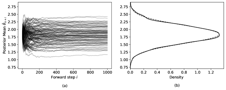
We now conclude this section with a concrete demonstration of the equivalence between posterior sampling and the forward sampling of through a simple normal model with unknown mean based on an example from Hahn, (2015).
Example 1
Let , with . Given an observed dataset , the tractable posterior density takes on the form where
The posterior predictive density then takes on the form . For observed data, we generated for with , giving .
We can plot the independent sample paths for the posterior mean, , as we recursively forward sample , where in this example. In Figure 1, we see that the sample paths of each converge to a random as increases, with the density of very close to the analytic posterior. From Doob’s consistency theorem, we know this is exact for .
2.2 The methodological approach
Through Doob’s result in Theorem 1, we have demonstrated the predictive view of Bayesian inference as a means to understand how the posterior uncertainty in arises from the missing information . The predictive view of Bayesian inference partitions posterior sampling into two distinct tasks. The first is the simulation of through the sequence of 1-step ahead predictive distributions to assess the uncertainty that arises from the missing observables. The second is the recovery of the parameter of interest from the simulated complete information, which is facilitated by the limiting posterior mean point estimate . The uncertainty in then flows from the uncertainty in . Inspired by this, we will now demonstrate the practical importance of this interpretation by introducing a predictive framework for inference built exactly on these two tasks. This framework eliminates the need for the usual likelihood–prior construction of the Bayesian model, and as such generalizes the traditional Bayesian posterior to the martingale posterior.
2.2.1 Sampling the missing data
For the predictive Bayesian, the role of the posterior is to aid in the updating of the predictive density, after observing , and the likelihood and prior can be viewed as merely intermediate tools to construct the sequence of predictives (Roberts,, 1965). To obviate the need of a likelihood-prior specification, our proposal is to specify the sequence of 1-step ahead predictive densities directly, which implies a joint density through the factorization
| (2.5) |
However, we must take care in our elicitation of to ensure the existence of the limit . As this is technical, we defer a formal discussion of this choice and the conditions required to Section 3. For now, we point out that a sufficient condition is for the 1-step ahead predictive densities to satisfy a martingale condition similar to that of Doob, with details given in Section 3.2. It may seem that constructing this sequence will incur too much complexity, but we will show this is in fact feasible and desirable. One key idea is to utilize a general sequential updating procedure whereby given an observed , we have a direct and tractable iterative update
2.2.2 Recovering the quantity of interest
We now discuss the second task: given a sample , we require a procedure to recover the quantity of interest. In a traditional parametric Bayesian model, the quantity of interest is usually the unknown parameter that indexes the sampling density, and as shown by Doob, the limiting posterior mean serves this purpose. A more general framework is the decision task discussed in Bissiri et al., (2016), where the aim is to minimize a functional of an unknown distribution function from which samples are i.i.d.. For some loss function , the quantity of interest is now defined as
| (2.6) |
More details can be found for example in Huber, (2004) and Bissiri et al., (2016). Typical examples are for the median, for the mean, and for the Kullback-Leibler minimizer between some parametric density and the sampling density . The choice of the negative log–likelihood is also interesting as it allows us to target the parameters of a parametric model without the assumption that the model is well–specified (Walker,, 2013; Bissiri et al.,, 2016). While misspecification under our framework is still an open question, the Bayesian bootstrap has particularly desirable theoretical and practical properties under misspecification (Lyddon et al.,, 2018, 2019; Fong et al.,, 2019). We will also consider more general forms of , e.g. the density of .
Working now in the space of probability distributions, the traditional Bayesian approach would be to elicit a prior on , perhaps nonparametric, and derive the posterior . Here, represents the Bayesian’s subjective belief on the unknown true . A posterior sample of is then obtained as follows: draw and compute the minimizing . For our generalization beyond the likelihood-prior construction, we do not have a posterior mean nor a posterior , and thus require an alternative to recover the quantity of interest given a sample of conditioned on . Our proposal is to construct the random limiting empirical distribution function
| (2.7) |
and take to minimize . Here, our takes the place of the posterior draw of , and its existence will rely on the martingale condition as mentioned above. We can write or interchangeably for the parameter of interest computed from the completed information. If we specify through the usual likelihood–prior construction, then sampling from the posterior in fact yields the same random distribution function as almost surely; this theoretical justification for the limiting empirical distribution function is in Appendix C.2.
2.3 The martingale posterior
Our framework for predictive inference is summarized as follows. Suppose we observe i.i.d. from some unknown and are interested in the defined by (2.6). We specify a sequence of predictive densities which satisfies the martingale condition to be discussed in Section 3.2 and implies a joint distribution through (2.5). We then impute an infinite future dataset through
for . Given the infinite random dataset and the corresponding empirical distribution function , we compute . We designate the distribution of as the martingale posterior, where we use the notation for comparability to traditional Bayes.
Definition 1 (Martingale posterior).
The martingale posterior distribution is defined as
| (2.8) |
for measurable set .
Drawing samples of from the martingale posterior involves repeating the above simulation procedure given above. We refer to this Monte Carlo scheme as predictive resampling, which has strong connections with the Bayesian bootstrap of Rubin, (1981), as we will see in Section 2.4. In practice however, we may be unable to simulate , or the study population may be of finite size . In this case, we can instead impute for finite , giving us the analogous empirical distribution function and parameter or .
Definition 2 (Finite martingale posterior).
The finite martingale posterior is similarly defined as
| (2.9) |
In the finite form, the role of the two constituent elements, and , is even clearer. For infinite populations, we also highlight that the value of varies around , but this may be negligible for sufficiently large . If the population is actually finite and of size , then would be the actual target and thus not an approximation. Finally, we reiterate that the martingale posterior (2.8) is equivalent to the traditional Bayesian posterior when using (1.2) as the predictive. A summary of the notation and an illustration of the imputation scheme is provided respectively in Appendices A, B.
2.4 The Bayesian bootstrap
The resemblance of the martingale posterior to a bootstrap estimator should not have gone unnoticed, as both involve repeated sampling of observables followed by computing estimates from the sampled dataset. The Bayesian bootstrap of Rubin, (1981) is often described as the Bayesian version of the frequentist bootstrap. After observing , one draws a random distribution function from the posterior through
| (2.10) |
A posterior sample of the statistic of interest can then be computed as . One interpretation of the Dirichlet weights is to generate uncertainty through the randomization of the objective function (Newton and Raftery,, 1994; Jin et al.,, 2001; Newton et al.,, 2020; Ng and Newton,, 2020). Closer to our perspective are the connections to Bayesian nonparametric inference, which have been explored in much detail within the literature as it is the non-informative limit of a posterior Dirichlet process (Lo,, 1987; Muliere and Secchi,, 1996; Ghosal and van der Vaart,, 2017). Recent work has exploited the computational advantages of the Bayesian bootstrap for scalable nonparametric inference; see Saarela et al., (2015); Lyddon et al., (2018); Fong et al., (2019); Newton et al., (2020); Knoblauch and Vomfell, (2020); Nie and Ročková, (2020).
2.4.1 The empirical predictive
Within the framework of martingale posteriors, the Bayesian bootstrap has a particularly elegant interpretation that follows from the equivalence to the Pólya urn scheme (Blackwell and MacQueen,, 1973; Lo,, 1988). The Bayesian bootstrap is equivalent to the martingale posterior if we define our sequence of predictive probability distribution functions to be the sequence of empirical distribution functions, that is
| (2.11) |
This is easy to see as sampling amounts to drawing with replacement 1 of colours with probability from the urn, and updating to is equivalent to reinforcing the urn, that is
Continuing on to , the proportions of colours converge in distribution to the Dirichlet distribution. Interestingly, this choice of predictive implies an exchangeable future sequence from the connection to the Dirichlet process. The atomic support of the predictive is however slightly problematic if is continuous, as any new observations from will be assigned a predictive probability of zero; we will introduce methodology that remedies this in Section 4. Generalizations to other atomic predictives can for example be found in Zabell et al., (1982); Muliere et al., (2000).
One can consider the empirical distribution function as the simplest nonparametric predictive for i.i.d. data, and can thus regard the Bayesian bootstrap as the simplest Bayesian nonparametric model. The uncertainty from the Bayesian bootstrap arises not from the random weights, but from the sequence of empirical predictive distributions. We resample with replacement, treating each resampled point as a new observed datum; this fundamental observation is our motivation for the term predictive resampling.
2.4.2 Comparison to the frequentist bootstrap
Throughout this section, we have assumed the existence of an underlying from which are i.i.d., which in turn implies the existence of an unknown true much like the frequentist. This has some connections to frequentist consistency under our framework, which we discuss in Section 6.3. The posterior random variable then represents our subjective uncertainty in after observing . The Bayesian bootstrap and Efron’s bootstrap (Efron,, 1979) are then ideal vessels for the contrasting of Bayesian and frequentist uncertainty. Both methods are nonparametric and begin by constructing the empirical predictive as in (2.11) from the atoms of as an estimate of , and both involve resampling. The key difference lies in how the resampling is carried out.
The frequentist draws a dataset of size i.i.d. from , which we write as with corresponding empirical distribution function , and computes as a random sample of the estimator. The Bayesian on the other hand draws an infinite future dataset through predictive resampling, and computes as a random sample of the estimand, where is the limiting empirical distribution function of , noting again that the Bayesian holds fixed. This is summarized in Algorithms 1 and 2. Notably, the specification in both bootstraps are equivalent: it is merely the elicitation of , which entirely characterizes both types of uncertainty.
2.5 Related work
There have been many others that shared de Finetti’s view on the emphasis on observables for inference. The work of Dawid, (1984); Dawid, 1992a ; Dawid, 1992b on prequential statistics, a portmanteau of probability/predictive and sequential, is one such example. In his work, Dawid focuses on the importance of forecasting, and introduces statistical methodology that assign predictive probabilities and assesses these methods on their agreement with the observed data. In particular, Dawid, (1984) recommends eliciting a sequence of 1-step ahead predictive distributions as we do, but motivates this by arguing that forecasting is the main statistical task. As pointed out in Section 1, this is in contrast to our case, where parameter inference is the main task of interest. We will see in Section 3.2 that stricter conditions are required on this sequence of predictives for inference. Another strong proponent of the predictive approach is the work of Geisser: he believed that the prediction of observables was of much greater importance than the estimation of parameters, which he described as “artificial constructs” (Geisser,, 1975). His emphasis on the predictive motivated cross-validation (Stone,, 1974; Geisser,, 1974), which is now popular for Bayesian model evaluation (Vehtari and Lampinen,, 2002; Gelman et al.,, 2014). Works such as Dawid, (1985); Lauritzen, (1988) also consider parameters as functions of the infinite sequence of observations using the notion of repetitive structures. Finally, the work of Rubin on both the potential outcomes model (Rubin,, 1974) and multiple imputation (Rubin,, 2004) highlights the idea of inference via imputation.
An early application of what is essentially finite predictive resampling and martingale posteriors is Bayesian inference for finite populations, first discussed in Roberts, (1965); Ericson, (1969) and later by Geisser, (1982, 1983). A finite population Bayesian bootstrap is described in Lo, (1988), in which a finite Pólya urn is used to simulate from the posterior. The ‘Pólya posterior’ of Ghosh and Meeden, (1997) uses the same approach following an admissibility argument. These methods have applications in survey sampling or the interim monitoring of clinical trials (Saville et al.,, 2014).
There have been recent exciting directions of work that investigate the predictive view of Bayesian nonparametrics (BNP). Fortini et al., (2000) investigate under what conditions parametric models arise from the sequence of predictive distributions using the concept of predictive sufficiency, and derive conditions such that the joint distribution is exchangeable. Fortini and Petrone, (2012, 2014) discuss the construction of a range of popular exchangeable BNP priors through a sequence of predictive distributions, motivated through a predictive de Finetti’s representation theorem (Fortini and Petrone,, 2012, Theorem 2). Berti et al., (2020) then generalize the nonparametric approach to c.i.d. sequences; we will later see that c.i.d. sequences, as introduced in Berti et al., (2004), play a crucial role in our work. However, the previously described methods are mostly constrained to the discrete case. Hahn, (2015) and Hahn et al., (2018) construct c.i.d. models through a predictive sequence for univariate density estimation, respectively utilizing the kernel density estimator and the bivariate copula. Hahn, (2015) also discusses the connection of Bayesian uncertainty and prediction with a weaker argument, and gives a similar example to our Example 1. Predictive resampling is then used to sample nonparametric densities from a finite martingale posterior; however Hahn, (2015) instead specifies the predictive distribution for large and works backwards to find the sequence of predictives. Fortini and Petrone, (2020) analyze the predictive recursion algorithm of Newton et al., (1998) and the implied underlying quasi-Bayesian model. In their work, they carry out predictive resampling to simulate from the prior law of the mixing distribution in an example, and obtain its asymptotic distribution under the c.i.d. model, that is an asymptotic approximation to the martingale posterior. An interesting aside is the recent work of Waudby-Smith and Ramdas, (2020) which utilizes adaptive betting with martingale conditions for the purpose of constructing frequentist confidence intervals. We aim to unify these related strands of research under a single framework.
3 Predictive resampling for martingale posteriors
For the martingale posterior, we now embark on the task of eliciting the general 1-step ahead predictive distributions, with the traditional Bayesian posterior predictive as a special case. For notational convenience, we write the sequence of predictive probability distribution functions estimated after observing as
| (3.1) |
which may have corresponding density functions . The subscript indicates the length of the conditioning sequence, and there may be a as some initial choice. For a general sequence of predictives, where exchangeability no longer necessarily holds, we instead define our joint distribution on through this sequence of 1-step ahead predictives and the chain rule as in (2.5). The Ionescu-Tulcea theorem (Kallenberg,, 1997, Theorem 5.17) guarantees the existence of such a joint distribution as we take , which has been pointed out by works such as Dawid, (1984); Fortini and Petrone, (2012); Berti et al., (2020).
Beyond the traditional Bayesian posterior predictive, there is good justification for specifying the model with 1-step ahead predictives, instead of say -step ahead. It is simple to interpret and estimate a 1-step ahead predictive as the decision maker’s best estimate of the unknown sampling distribution function , and methods such as maximum likelihood estimation already do this. There are also connections with forecasting and prequential statistics (Dawid,, 1984). Finally, we will see that a 1-step update of the predictive allows for the enforcing of the c.i.d. condition for predictive coherence.
While the prescription of (3.1) remains a subjective task, we find it to be no more subjective than the selection of a likelihood function. There is no longer a need to elicit subjective distributions on parameters which merely index the sampling distribution with no physical meaning, which has been described as ‘intrinsic’ (Dawid,, 1985). In nonparametric inference, we also do not need to elicit priors directly on the space of probability distributions, which can be cumbersome. The uncertainty arises simply from the elicitation of (3.1). It is clear that we can still use external information and subjective judgement not provided by the data in this construction.
3.1 A practical algorithm for uncertainty
Given the model specification (3.1), suppose we wish to undertake inference on a statistic of interest , defined through a loss function as in (2.6). We can obtain finite martingale posterior samples through predictive resampling given in Algorithm 3, noting the similarity to the Bayesian bootstrap algorithm.
In summary, we run a forward simulation starting at by consecutively sampling from the 1-step ahead predictives and updating as we go. For large , we now have a random dataset from which we can compute the empirical distribution function and statistic of interest . In particular, only when the sequence of predictives takes on the form (1.2), combined with the self-information loss, , is this procedure equivalent to traditional Bayesian inference.
The empirical distribution is atomic, which may be problematic if the object of interest requires the limiting to be continuous, for example if is the probability density of or a tail probability. In this case, we can instead compute , where is the random predictive distribution function conditioned on , which would typically be continuous. We can regard as the finite approximation to the limiting predictive distribution function , which serves the same purpose as the limiting empirical in Section 2.2.2. In fact, and coincide for traditional Bayesian models, and even for the more general c.i.d. sequence of predictives that we will consider shortly. We discuss this in Appendix C, borrowing results from Doob, (1949), Berti et al., (2004) and Lijoi et al., (2004).
Some experimental and theoretical guidance for selecting a sufficiently large to estimate is given in Sections 5 and 6. However, it is also interesting to consider a finite population, where the of interest is indeed the empirical distribution function of a population of size , as discussed in Sections 2.3 and 2.5. In this case, truncating predictive resampling at indeed returns the correct uncertainty in any parameter of interest of the finite population.
3.2 Predictive coherence and conditionally identically distributed sequences
The notion of coherence on one’s belief on the parameter is key to the subjective Bayesian, where coherence may be defined in a decision-theoretic sense (Bernardo and Smith,, 2009, Chapter 2.3) or through Dutch book arguments (e.g. Heath and Sudderth, (1978)). Extensions of coherence to forecasting are given in Lane and Sudderth, (1984); Berti et al., (1998), and more examples of coherence in general can be found in Robins and Wasserman, (2000); Eaton and Freedman, (2004). More recently, the notion of coherence of belief updating was introduced in Bissiri et al., (2016), where a belief update on a statistic of interest is coherent if the update is equivalent whether computed sequentially with followed by or with in tandem through an additive loss condition. In bypassing the traditional likelihood-prior construction, we must forsake the usual coherence of belief updating and exchangeability. Instead, we specify conditions for a valid martingale posterior entirely in terms of the predictive distribution function, which we term predictive coherence.
Suppose we observe i.i.d. from some and construct as in (3.1). We can then view the predictive machine as the best estimate of the unknown distribution function from which the data arose, incorporating all observed data and any possible subjective knowledge. The first minimal condition is that the sequence of predictive distribution functions converges to a random distribution function. Secondly, we would ensure that predictive resampling does not introduce any new information or bias, as is already our best summary of the observed , and the procedure should merely return uncertainty. Formally, we write these conditions respectively as follows:
Condition 1 (Existence).
The sequence converges to a random almost surely for each , where is a random probability distribution function.
Condition 2 (Unbiasedness).
The posterior expectation of the random distribution function satisfies
almost surely for each .
Under Condition 1, is defined through the sequence of predictives, and we can thus treat directly as the random distribution function without the need for an underlying Bayes’ rule representation. This in turn gives us the posterior uncertainty in any statistic . Condition 2 is stricter, and implies that is our best estimate of and is equal to the posterior mean.
Fortunately, Conditions 1 and 2 are satisfied if the sequence is conditionally identically distributed (c.i.d.), as introduced and studied in Berti et al., (2004). Many useful properties of c.i.d. sequences have been shown in their work, which we now summarize. The sequence is c.i.d if we have
almost surely for each . This states that conditional on , any future data points will be identically distributed according to the predictive . This predictive invariance is particularly natural as a minimal predictive coherence condition, and serves as an analogue to de Finetti’s exchangeability assumption in the predictive framework. In fact, as shown in Kallenberg, (1988), the c.i.d. condition is a weakening of exchangeability, and Berti et al., (2004) also show that c.i.d. sequences are asymptotically exchangeable, which we state formally in Theorem 3 in Section 6.1.
An equivalent formulation of c.i.d. sequences which connects closely to the predictive coherency conditions is that is a martingale for , that is
| (3.2) |
almost surely for each , noting that depends on as in (3.1). Relying again on Doob’s martingale convergence theorem (Doob,, 1953), the sequence converges to almost surely for each , and can be shown to be a random probability distribution function (Berti et al.,, 2004); we state this formally in Theorem 4 in Section 6.1. In this case, we also designate the distribution of as the martingale posterior when we do not specify . Condition 2 is then satisfied as the sequence is uniformly integrable. Furthermore, we are guaranteed the existence of the limiting empirical distribution function as required in Section 2.2.2, and in fact almost surely so the interchangeability of and is justified. This equivalence, as well as the convergence of with for a certain class of parameters, is discussed in Appendix C.1. Although not explored here, connections of the c.i.d. property to other notions of coherence, such as those given at the start of this subsection, would be interesting to investigate especially given the absence of the prior distribution.
Although the above predictive coherence conditions are for a valid martingale posterior, we still need to specify a sequence of predictive distributions. Clearly the traditional Bayesian posterior predictive satisfies the above conditions, but in the interest of computational expediency or the desire to bypass the likelihood-prior construction, we may wish to consider more general predictive machines. The remainder of this paper will consider recursive predictive densities using bivariate copulas.
4 Recursive predictives with bivariate copulas
In this section, we focus primarily on the elicitation of the sequence of predictives (3.1) in the continuous case, where is the density of in (3.1). Analogous predictives are derivable for the discrete case, and these are obtained in Berti et al., (2020). In particular, we investigate the prescription of this sequence of predictives through a recursive manner, that is for
where is a sequence of update functions, possibly parameterized by a hyperparameter . In this case, we require an initial guess for our recursion, which plays the role of a prior guess on . A recursive update of this form is not necessary for a martingale posterior, but it allows for simple satisfaction of conditions for predictive coherence as discussed in Section 3.2, and computations for predictive resampling will also be significantly easier. Furthermore, when one is only interested in estimating , recursive updates may have computational advantages as one does not need to explicitly estimate the posterior.
Recursive updates have previously been motivated as a fast alternative to MCMC in Dirichlet process mixture models (DPMM). The predictive recursion algorithm was first introduced by Newton et al., (1998), which estimates the mixing distribution through a recursive update, and its properties have been studied in detail in the literature; see Martin, (2018) for a thorough review. One interesting property shown in Fortini and Petrone, (2020) is that the sequence of observables in Newton’s algorithm is c.i.d.; however, the computation of the predictive densities is intractable and requires numerical integration, so we will not discuss this method further here. Direct recursive updates for the predictive density were then introduced in Hahn, (2015); Hahn et al., (2018); Berti et al., (2020), all of which satisfy the c.i.d. condition. The bivariate copula method of Hahn et al., (2018) is particularly tractable and well motivated, and we will now build on this method in this section.
4.1 Bivariate copula update
To satisfy the c.i.d. condition required for predictive coherence, we can extend the martingale condition to hold for the sequence of densities such that for
| (4.1) |
almost surely for each , assuming the expectations exist. We highlight again that depends on as it is the density of (3.1). The above is a sufficient condition for (3.2) to hold, so our sequence is c.i.d. and the existence and unbiasedness conditions are satisfied giving us a valid martingale posterior. In fact, the martingale convergence theorem shows that almost surely for each , but more assumptions are needed to show that is the density of ; we explore this in Theorem 5 in Section 6.1.
One particular tractable form of update rule that satisfies (3.2) is the bivariate copula (Nelsen,, 2007) update interpretation of Bayesian inference first introduced in Hahn et al., (2018) for univariate data. A bivariate copula is a bivariate cumulative distribution function with uniform marginal distributions, and in the cases we consider it will have a probability density function . The bivariate copula can be regarded as characterizing the dependence between two random variables independent of their marginals, which can be seen through Sklar’s theorem in the bivariate case.
Theorem 2 (Sklar, (1959)).
For a bivariate cumulative distribution function with continuous marginals , there exists a unique bivariate copula such that
Furthermore, if has a density with marginal densities , we can write
where is the density of .
This holds for higher dimensions, but we state it for as this is what we will be working with. From this, we can see that the bivariate copula can model the dependence structure between consecutive predictive densities, and thus we have the following corollary, with the proof given in Appendix D.1.
Corollary 1.
The sequence of conditional densities satisfies the martingale condition (4.1) if and only if there exists a unique sequence of bivariate copula densities such that
| (4.2) |
for and is the distribution function of .
In the univariate case, we can thus elicit a c.i.d. model through a sequence of copulas, that is we have (4.2) as our update function . We highlight that is the bivariate copula density that models the dependence between conditioned on . Although the sequence can technically depend arbitrarily on (and the sample size ) without violating the martingale condition, we will later constrain this dependence. As all exchangeable Bayesian models are c.i.d., there exists a unique sequence of copulas which may or may not be tractable that characterize the model (Hahn et al.,, 2018). This sequence takes on exactly the form
| (4.3) |
The copula density arises following Theorem 2 as the numerator in (4.3) is the joint density with marginal densities and . Instead of specifying the likelihood and prior, we will now consider the specification of the sequence of copulas directly. The form for inspired by the DPMM is particularly attractive, and serves well as the canonical extension of the Bayesian bootstrap predictive to continuous random variables. In the remainder of this section, we will first review the method of Hahn et al., (2018) for univariate density estimation, and extend the methodology to include predictive resampling and hyperparameter selection. We then introduce analogous copula updates for more advanced data settings, including multivariate density estimation, regression and classification.
4.2 Univariate case
Tractable forms of this sequence of copulas in Bayesian models are investigated in Hahn et al., (2018), which correspond to conjugate priors. The update of particular interest is that of the DPMM (Escobar and West,, 1995) of the particular form
| (4.4) |
where is the scalar precision parameter that we set to . The model is nonparametric, making it a strong candidate for a predictive update, but only the copula update for is tractable. Inspired by this first update step, Hahn et al., (2018) suggest that the general update to compute the density after observing for takes on the form
| (4.5) | ||||
where is the distribution function of . Here is the bivariate Gaussian copula density and is the conditional Gaussian copula of the forms:
| (4.6) |
where is the standard inverse normal distribution function and is the standard bivariate density with correlation . The role of as a bandwidth will be explored shortly. The update (4.5) is then a mixture of the independent copula density and the Gaussian copula density, and the sequence ensures the update approaches the independent copula as . Although asymptotic independence is not necessary for the martingale condition, this property holds for Bayesian sequences of copulas (Hahn et al.,, 2018), and is indeed important for frequentist consistency when estimating as we will see in Section 6.3. We will see the specific suggested form of at the end of this subsection.
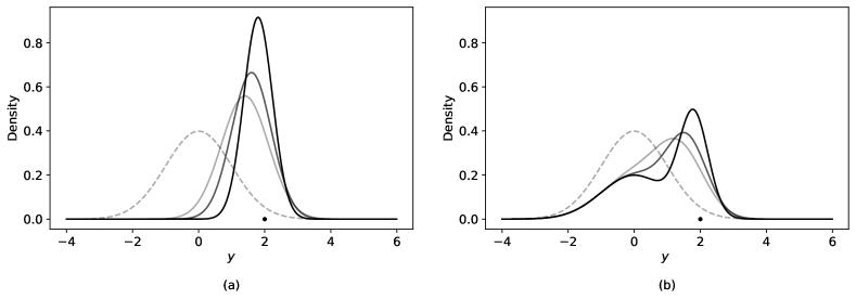
Note the similarity of the update in (4.5) to the generalized Pólya urn for the Dirichlet process, which for has the update . We can thus interpret (4.5) as a smooth generalization of the Bayesian bootstrap update for continuous distributions. One can also interpret (4.5) as a Bayesian kernel density estimate (KDE) that satisfies the c.i.d. condition, as the regular KDE cannot satisfy this condition (West,, 1991). The update can be visualized in Figure 2, where for convenience we write . The Gaussian copula kernel is a data dependent kernel roughly centered at , as shown in the left. The kernel becomes sharper as increases, and we recover the Bayesian bootstrap in the limit of (with ). The update is then a mixture of and the copula kernel, which gives us in the right panel.
The recursive update was first introduced to compute , but properties of the update make it a highly suitable candidate for predictive resampling. Firstly, by Corollary 1, this update is guaranteed to provide a c.i.d. sequence and hence satisfy the existence and unbiasedness conditions. Secondly, the update of the predictive distribution is online, and does not require an expensive recomputation of the predictive distribution at each step. Finally, the predictive resampling update is particularly computationally elegant as implies that , so all that is required is the simulation of uniform random variables. The forward sampling step then involves simulating and computing
| (4.7) | ||||
iterated over , which gives us a random at the end. There is no need to actually sample , which is possible but is more computationally expensive. In Section 6, we will see that this update form allows easy analysis of the theoretical properties of predictive resampling.
The bandwidth controls the smoothness of the density estimate, which we can set in a data-dependent manner as we show in Section 4.5.2. On the other hand, the sequence is responsible for the uncertainty as we will see in Section 6, so extra care must be taken when eliciting this. Hahn et al., (2018) suggest the form inspired from the stick-breaking process of the posterior DP as in the Bayesian bootstrap, which works well for estimating but we find this performs poorly when predictive resampling, giving too little uncertainty. This was also observed in Fortini and Petrone, (2020) in the case of Newton’s recursive method. However, it should be observed that the posterior over the mixing distribution is actually a mixture of DPs, that is
where is intractable. As shown in Appendix E.1.1, we only require the simplifying assumption of , which corresponds to each datum belonging to its own cluster in a similar spirit to the KDE. This then returns us the same copula update as (4.5) with
| (4.8) |
Intuitively, the additional mixing over results in the inflated value compared to . Note this is still , matches with initial update step for , and works much better in practice as it approaches more slowly. We use this sequence for the remainder of the copula methods.
4.3 Multivariate case
In this section, we extend the univariate method to multivariate data , allowing us to both learn recursively, and retain the c.i.d. sequence so we can predictively resample to obtain uncertainty. Even without predictive resampling, a general multivariate density estimator is of interest, as the KDE is known to perform poorly in high dimensions; see Wang and Scott, (2019) for a review. Computation for the multivariate DPMM (MacEachern,, 1994; Escobar and West,, 1995; Neal,, 2000) may scale poorly as the number of dimensions grows. Variational inference (VI) is a quicker approximation as demonstrated in Blei and Jordan, (2006), but there is strong dependence on the optimization procedure, which may impair performance in high dimensions. A copula method for bivariate data is suggested in the appendix of Hahn et al., (2018), but it does not scale well with dimensionality and is not c.i.d.. A recursive method for multivariate density estimation is introduced in Cappello and Walker, (2018), but numerical integration on a grid is still required, which scales exponentially with , or a Monte Carlo scheme is required. Fortini and Petrone, (2020) propose a multivariate extension of Newton’s recursive method, but it also requires an approximate Monte Carlo scheme to evaluate the predictive density.
Extending the above argument in Corollary 1 to multivariate data is not as straightforward, as we would like to factorize the joint density into , which does not have the copula interpretation like in the 2-dimensional case. Furthermore, building high-dimensional copulas is a difficult task, and bivariate copulas are good building blocks for higher dimensional dependency (Joe and Xu,, 1996; Bedford and Cooke,, 2001; Aas et al.,, 2009).
4.3.1 Factorized kernel
With the above in mind, we now consider the first step update of a multivariate DPMM below
| (4.9) |
where is the -th dimension of , and likewise for . Note the factorized normal kernel and independent priors for each . From this, we see that we can factorize . It is shown in Appendix E.1.2 that the first update step takes on the form
where is the -th dimension of the -th data point. However, naively using this update for will result in the sequence no longer satisfying the martingale condition in (4.1), and we also find that it performs poorly empirically. A simple but key extension allows us to retain the c.i.d. sequence:
| (4.10) |
where
The input to the bivariate normal copula is now the conditional cumulative distribution function at and for a particular dimension ordering, and this change ensures many desirable properties. First, we can verify that the martingale condition (4.1) now holds through a multivariate change of variables from to , so the c.i.d. condition is satisfied. By marginalizing in descending order, we also have that the marginals for a single ordering of dimensions has the same update
| (4.11) |
From this, we can update the conditional distribution functions via
| (4.12) |
and likewise for . As a result, all terms in the update (4.10) can be computed tractably, with no need for numerical integration or approximations, allowing us to extend this method to any number of dimensions as computation complexity is linear in . Notably, we must specify an ordering of the dimensions of , which at first may seem undesirable. However, it is not an assumption on dependence, and the only implication is that the subset of ordered marginal distributions continue to satisfy (4.11), that is a sort of marginal coherence. Interestingly, the form of (4.11) suggests that depends only on the first dimensions of . Practically, we find the dimension ordering makes little difference, and we recommend selecting the ordering such that any conditional or marginal distributions of interest remain tractable. In Appendix E.1.3 we provide an extension to the above for mixed-type data.
Predictive resampling again takes on a simple form due to the nature of the update (4.10). We can imagine drawing each dimension of in a sequential nature, that is
| (4.13) |
Denoting , we then have that for , which we can substitute into (4.10) and (4.12), similar to the univariate case. Predictive resampling again only requires sampling independent uniform random variables for each forward step and computing the update.
4.4 Regression
We now consider extending the copula method and predictive resampling to the regression setting, where we have univariate (which can be easily extended to multivariate) with corresponding covariates , where for example . We will later also consider binary regression, where . One assumption is that the covariates are random, where we write , and we are interested in . We term this the ‘joint method’, as we infer the full joint from which the conditional then follows. Examples of this are Müller et al., (1996); Shahbaba and Neal, (2009); Hannah et al., (2011), where the prior on is a DPMM. The second type of assumption, which we call the ‘conditional method’, is the more common framework. Here we assume that are fixed design points and the randomness arises from the response , so we infer a family of conditional densities . The most common framework is the additional assumption of , where are independent zero-mean noise, and a prior on the mean function is assumed, e.g. a Gaussian process (Rasmussen,, 2003). Alternatively, one can elicit a prior on directly, for example with mixture models based on the dependent Dirichlet process (MacEachern,, 1999). We recommend Wade, (2013); Wade et al., (2014); Quintana et al., (2020) for thorough reviews.
4.4.1 Joint method
The joint method follows easily from the multivariate: we first estimate the joint predictive density , then compute the conditional . Utilizing (4.11), we have the tractable update for the conditional density
| (4.14) |
where
| (4.15) | ||||||
Here, we can have separate bandwidths for and , and even one for each dimension of . The updates for are the same as in (4.12), and again all terms are tractable. Predictive resampling in this case requires simulating both just like in (4.13).
4.4.2 Conditional method
When is high-dimensional, it may be cumbersome to model when we are only interested in the conditional density. The conditional method models directly, and we turn to the dependent Dirichlet process (DDP) and its extensions for inspiration. In particular, consider the general covariate-dependent stick-breaking mixture model
| (4.16) |
where follows an -dependent stick-breaking process, and . A full derivation is provided in Appendix E.2.2. We can show that the update step of the predictive takes the form
| (4.17) |
where , and are as in (4.15). The term is tractable for some choices of the construction of , e.g. the kernel stick-breaking process (Dunson and Park,, 2008). Unfortunately this does not provide guidance on how to generalize to . Instead, we turn to the joint copula method in the previous section for inspiration, which can be written as (4.17) with
This form of can be viewed as a distance measure between and that is dependent on which is updated in parallel. To avoid modelling , we can simplify the above and consider the following as a distance function directly:
| (4.18) |
which is equivalent to the joint method but leaving without updating, providing us an increase in computational speed. This form requires to be standardized for good performance, and we find that specifying independent bandwidths for each dimension in works well. This method is similar to the normalized covariate-dependent weights of Antoniano-Villalobos et al., (2014).
If is indeed a subsequence of a deterministic sequence of design points , then predictive resampling simply involves selecting for from this sequence, and drawing . If is actually random and we have chosen the conditional approach simply for convenience, then we can draw the future from the sequence of empirical predictives as in the Bayesian bootstrap. We have however noticed some numerical sensitivity to this choice of in the uncertainty in for far from the observed dataset; this is illustrated in Appendices G.5 and G.6. Once again, conditional on , we have that , so predictive resampling only consists of simulating independent uniform random variables and updating. An example of using the Bayesian bootstrap for the covariates is provided in Appendix G.6.
4.4.3 Classification
For classification, both the joint and conditional approach generalize easily to when . To this end, we can derive the copula update for a beta-Bernoulli mixture. As shown in Appendix E.3, this gives
| (4.19) |
where and . We can simply replace the bivariate Gaussian copula density in (4.14) and (4.17) with . One can check that is indeed a martingale when predictive resampling, and forward sampling can be done directly as drawing binary from the Bernoulli predictive is straightforward. Unfortunately, we do not have the useful property of in the discrete case, so predictive resampling beyond the Bayesian bootstrap for is computationally expensive at , or approximation via a grid is required. The Bayesian bootstrap for is still feasible as we only need to compute at the observed . An example of this method is provided in Appendix G.5.
4.5 Practical considerations
In this subsection, we discuss some practical considerations. Further details, such as those regarding sampling and optimization, are given in Appendix F.
4.5.1 Initial density
For the copula methods, we require an initial guess to begin our recursive updates, which can contain prior information. As it is a statement on observables, it is easier to elicit than a traditional Bayesian prior. In practice, we recommend standardizing each variable in the data to have mean and variance and using the default initialization for each dimension in an empirical Bayes fashion. For discrete variables, a suitable default choice is the uniform distribution over the classes. Finally, in the regression case, we can include prior information on the regression function, e.g. . However, tends to work well as a default choice.
4.5.2 Hyperparameters
As we recommend the fixed form of in (4.8), the only hyperparameter in the copula update is the constant which parameterizes the bivariate normal copula in (4.6). While Hahn et al., (2018) suggest a default choice for , we prefer a data-driven approach. Fortunately, there is an obvious method to select using the prequential log score of Dawid, (1984), that is to maximize for density estimation or for regression, which is related to a cross-validation metric (Gneiting and Raftery,, 2007; Fong and Holmes,, 2020). This fits nicely into our simulative framework, as is selected on how well the sequence of predictives forecasts consecutive data points, which then informs us on the future predictives for predictive resampling. We can also specify a separate for each dimension, which corresponds to differing length scales for the update from each conditional distribution. For optimization, gradients with respect to can be computed quickly using automatic differentiation.
4.5.3 Permutations
Due to our relaxation of exchangeability in Section 3.2, one downside to the copula update and c.i.d. sequences in general is the dependence of on the permutation of when there is no natural ordering of the data. For permutation invariance, we can average and the corresponding prequential log-likelihood over random permutations of . We find in practice that is sufficient, which is computationally feasible for moderate due to the speed of the copula update, and the method is also parallelizable over permutations. For predictive resampling, we then begin with the permutation averaged and forward sample with the copula update. From asymptotic exchangeability in Theorem 3 in Section 6.1, averaging over permutations is not required for forward sampling provided is chosen to be sufficiently large. Theoretical properties of permutation averaging are explored in Tokdar et al., (2009); Dixit and Martin, (2019), which we do not consider here.
4.5.4 Computational complexity
For computing in the multivariate copula method, there is an overhead of first computing for , using (4.12), which requires operations, followed by operations to compute at a single (which is then parallelizable). After computing , predictive resampling future observables requires for each sample of ; this is fully parallelizable across test points and posterior samples. Interestingly, we first compute and only predictively resample after if uncertainty is desired, allowing for large computational savings if we are only interested in prediction. The regression methods have a similar computational cost.
5 Illustrations
In this section, we demonstrate the martingale posteriors induced by the copula methods of the previous section. Code for all experiments is available online at https://github.com/edfong/MP. We will demonstrate the copula method on examples where is the density itself or the loss function induces a simple parameter, e.g. quantiles. However, any of interest (as in Section 2.2.2) can technically be computed directly from the density or from and samples of , although this may require a high-dimensional grid or relatively expensive sampling. As a result, for cases with complex loss functions that do not rely on the smoothness of (e.g. a parametric log-likelihood), we recommend the Bayesian bootstrap instead as a computationally efficient predictive resampling approach. For examples regarding the Bayesian bootstrap, we refer the reader to the references in Section 2.4, and we qualitatively compare the Bayesian bootstrap and the copula methods in Section 7.
For all examples, we follow the recommendations of Section 4.5 for and averaging over permutations. We will demonstrate the monitoring of convergence to , but we set as a standard default for the number of forward samples, where is the size of the dataset. All copula examples are implemented in JAX (Bradbury et al.,, 2018), which is a Python package popular in the machine learning community. JAX is ideal for our copula updates: its just-in-time compilation facilitates a dramatic speed-up for our iterative updates especially on a GPU, and its efficient automatic differentiation allows for quick hyperparameter selection. Note that the first execution of code induces an overhead compilation time of between 10-20 seconds for all examples. We carry out all copula experiments on an Azure NC6 Virtual Machine, which has a one-half Tesla K80 GPU card. The copula methods consist of many parallel simple computations on a matrix of density values, which is very suitable for a GPU, unlike traditional MCMC. The DPMM with MCMC examples are implemented in the dirichletprocess package (Ross and Markwick,, 2018), which utilizes Gibbs sampling. Other benchmarks are implemented in sklearn (Pedregosa et al.,, 2011). Unless otherwise stated, default hyperparameter values are set for baselines. As the baseline packages are designed for CPU usage, we run them on a 2.6 GHz 6-Core Intel Core i7-8850H CPU. Further details can be found in Appendix G.2.
5.1 Density estimation
5.1.1 Univariate Gaussian mixture model
We begin by demonstrating the validity of the martingale posterior uncertainty returned from predictive resampling by comparing to a traditional DPMM in a simulated example, where the true density is known. We also discuss the monitoring of convergence of predictive resampling. For the data, we simulate and samples from a Gaussian mixture model:
For all plots, we compute the copula predictive on an even grid of size . Figures 3 and 4 show the martingale posterior density using the copula method for and respectively, compared to the traditional DPMM of Escobar and West, (1995) with MCMC. We draw samples for both methods. We see that the resulting uncertainty and posterior means are comparable between the copula and DPMM, and the uncertainty decreases as increases. The true density is largely contained within the 95% credible intervals.
For predictive resampling with the copula method, we judge convergence by considering the distance between the forward sampled and initial . This is demonstrated in Figure 5 for a single forward sample for . On the left, we have a numerical estimate of which converges to a constant, and likewise for on the right, where is the norm and is computed on the grid. We see in this example that is sufficiently large for to approximate . When we are not plotting on a grid and instead predicting over some test set, we may instead monitor
Optimization of the prequential log-likelihood gives us the optimal hyperparameter and for and respectively. The prequential log-likelihood is returned easily from the copula method, allowing for easy hyperparameter selection. However, computing the marginal likelihood for the DPMM is non-trivial, and thus setting the hyperparameters of the priors in a data-driven way, that is empirical Bayes, remains a difficult task. Here, we select the DPMM hyperparameters to match the smoothness of the posterior mean of the copula method for comparability of the uncertainty.

(b) for the DPMM, for with true density ( ) and data ( )
(b) for the DPMM, for with true density ( ) and data ( )

5.1.2 Univariate galaxy dataset
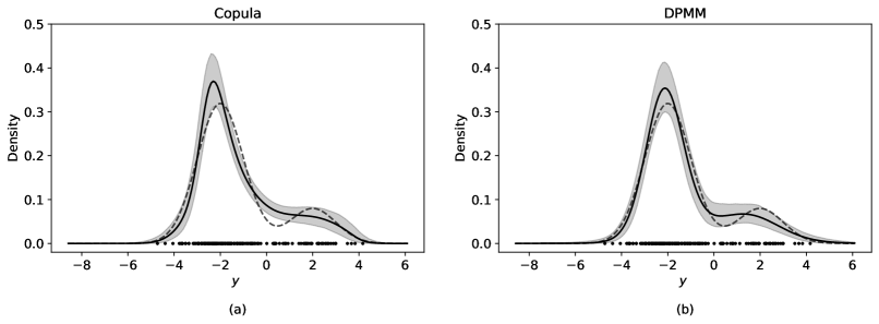
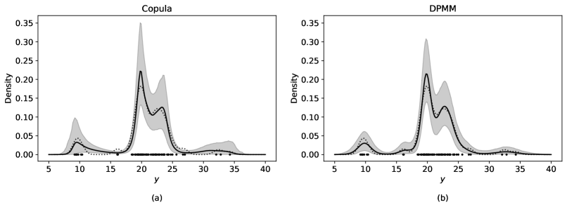
We now demonstrate the martingale posterior sampling of a parameter of interest that requires a smooth density, through predictive resampling and the computation of . We analyze the classic ‘galaxy’ dataset (Roeder,, 1990), thereby extending the example of Hahn et al., (2018) to the predictive resampling framework. The dataset consists of velocity measurements of galaxies in the Corona Borealis region. For all plots, we compute on an even grid of size , and unnormalize after the copula method so that the scale of is in km/sec.
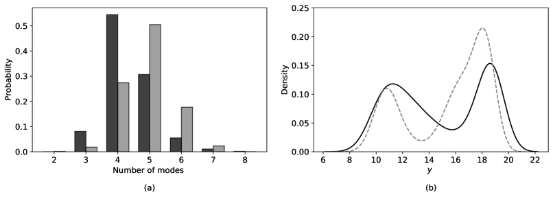
Figure 6 compares predictive resampling with the copula method for posterior samples of , where the selected bandwidth is . The bandwidth for KDE was computed through 10-fold cross-validation, and DPMM hyperparameters are set to the suggested values in West, (1991). The 95% credible intervals and posterior mean of the copula approach are comparable with that of the DPMM. Excluding compilation times, the optimization for and computation of on the grid of size took 0.5 seconds, and predictive resampling took 2 seconds. In comparison, DPMM with MCMC took 25 seconds for the same number of samples (), where the samples are not independent; the plots for MCMC are thus produced with . Given this random density, we can also compute the statistics of interest directly from the grid of density values. Martingale posterior samples of the number of modes and 10% quantiles of the random density are shown in Figure 7, with comparison to the DPMM. Here the copula method tends to prefer 4 modes, whereas the DPMM prefers 5.
(b) for the DPMM, with KDE ( ) and data ( )
(b) Posterior density of 10% quantiles for the copula method ( ) and the DPMM ( )
5.1.3 Bivariate air quality dataset
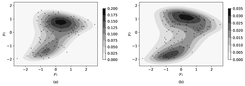
We demonstrate the martingale posterior for bivariate data using the method of Section 4.3.1, which has large computational gains over posterior sampling with DPMM when the density is of interest, where the latter is expensive due to dimensionality. For this, we look at the ‘airquality’ dataset (Chambers,, 2018) from DPpackage. The dataset consists of daily ozone and solar radiation measurements in New York, with completed data points. For all plots, we compute on a grid of size .
We fit the multivariate copula method of Section 4.3.1 with one bandwidth per dimension, and optimizing the prequential log-likelihood returns . Predictive resampling martingale posterior samples returns us the martingale posterior mean and standard deviation of the bivariate density as shown in Figure 8. Again excluding compilation times, the optimization for and computation of on the grid of size took 1 second, and predictive resampling took 10 seconds in total. For comparison, the DPMM with MCMC required 4 minutes for the same number of samples. Further details and comparisons to the DPMM are given in Appendix G.4.
Figure 9 plots a martingale posterior sample of the density, with the corresponding distance convergence plot. We see that is again sufficient, which suggests a dimension independent convergence rate of . This is justified in the theory in Section 6.

5.1.4 Multivariate UCI datasets
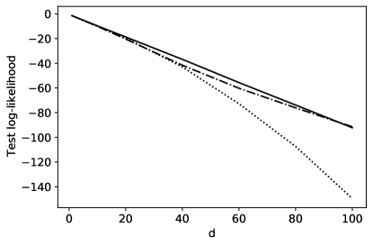
In this section, we demonstrate the multivariate copula method of Section 4.3.1 as a highly effective density estimator compared to the usual DPMM, as we do not need to deal with the posterior sampling or integration over high-dimensional parameters. We demonstrate on multivariate datasets from the UCI Machine Learning Repository (Dua and Graff,, 2017). To prevent misleadingly high density values, we remove non-numerical variables and one variable from any pairs with Pearson correlation coefficient greater than (e.g. see Tang et al., (2012)). We compare to the KDE, DPMM and multivariate Gaussian, and evaluate the methods with a 50-50 test-train split and average the test log-likelihoods over 10 random splits.
For the copula method, we use a single value of for all dimensions for a fair comparison to the KDE. We find that having distinct slightly improves predictive performance at the cost of higher optimization times. For the KDE, we use a single scalar bandwidth set through 10-fold cross-validation. For the DPMM, we set the Gaussian kernel to have diagonal covariance matrices and use VI (Blei and Jordan,, 2006). Using a full covariance matrix kernel is unreliable likely due to local optima for VI, and MCMC is too computationally expensive for large . For the multivariate Gaussian, we use the empirical mean and covariance.
| Dataset | Gaussian | KDE | DPMM (VI) | Copula | ||
|---|---|---|---|---|---|---|
| Breast cancer | -13.0 | |||||
| Ionosphere | -21.5 | |||||
| Parkinsons | -9.9 | |||||
| Wine | -14.6 |
As shown in Table 1, the performance is significantly better on test data for these datasets. The better performance than the KDE is likely due to the regularizing effect of , which is important here as is only of moderate size. The DPMM (VI) likely performs poorly as the diagonal covariance cannot capture dependent structure, and the number of variational parameters is still high so optimization is difficult. We provide a more detailed analysis of the degradation in performance with dimensionality of the DPMM with VI in Appendix G.7, where the copula method remains robust to dimensionality.
Overall, the run-times for the copula method, KDE and DPMM (VI) are similar, all of which are orders of magnitude faster than the DPMM with MCMC. For a single train-test split, the slowest example of the above (Breast cancer) for the copula method required less than 4 seconds in total to optimize , while computing the overhead and predicting on the test data required less than 100ms. For the same example, the KDE and DPMM (VI) required around 1.5 and 6 seconds respectively.
5.2 Regression and classification
5.2.1 Regression in LIDAR dataset
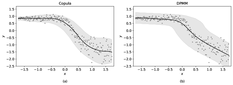
We now demonstrate the joint copula regression method of Section 4.4.1 on a non-linear heteroscedastic regression example, where the copula method performs well off-the-shelf. We use the LIDAR dataset from Wasserman, (2006), which consists of observations of the distance travelled by the light and the log ratio of intensity of the measured light from the two lasers; the latter is the dependent variable. For the plots below, we evaluate the conditional density on a grid of points.
For the copula method, we optimize the prequential conditional log-likelihood over the permutations, and get . The predictive mean and 95% central interval of are shown in Figure 10, compared to the DPMM, and we observe that the copula methods handle the nonlinearity better. The optimization, fitting and prediction on the grid took under 4 seconds for the copula method, compared to 5 minutes for the DPMM with MCMC for the same number of samples.
In Figure 11, we see martingale posterior samples of for the copula method compared to the DPMM. For reference, predictive resampling the martingale posterior samples on the grid for a single took under 3 seconds. One can see in Figure 11 that there is more posterior uncertainty in the density for the copula methods, as the DPMM has a simpler mean function (weighted sum of linear). Convergence of the conditional density under predictive resampling is now dependent on the value of . Figure 13(b) shows the distances as before for ; however, we find that more forward samples are needed for far from the data. Figure 12 then shows martingale posterior samples of where is far from the data, and we see that both the copula and DPMM method have larger uncertainty as expected. However, predictive resampling for the conditional copula method of Section 4.4.2 does not always demonstrate this desirable behaviour for outlying ; the joint and conditional methods are compared in Appendix G.6 and this undesirable behaviour is noted in the next experiment.
One may also be interested in the uncertainty in a point estimate for the function which we write as , in this case the conditional median. In Figure 13(a), we plot the martingale posterior mean and 95% credible interval of the conditional median of , where we see the uncertainty increasing with . Here we predictively resample on a grid of size and compute the median numerically; this took 12 seconds for samples.


5.2.2 Multivariate covariates in UCI datasets
We now demonstrate the conditional copula method for prediction in the regression and classification setting with multivariate covariates, which is of particular interest to the machine learning community. For high-dimensional covariates, the conditional copula method performs better than the joint method, both in terms of computational speed and test log-likelihood. This is likely due to the dominance of estimating in high dimensions, which disrupts the estimate of .
Similar to the multivariate density estimation, we demonstrate the regression and classification conditional copula methods on UCI datasets with scalar and multivariate . Again, we evaluate the methods with 10 random 50-50 test-train splits and evaluate the average test conditional log-likelihoods. We convert categorical variables into dummy variables, and report the preprocessed covariate dimensionality in Table 2. We compare to Bayesian linear regression and Gaussian processes (GP) with a single length scale RBF kernel as baselines for regression, and similarly to logistic regression and GPs with the logistic link and Laplace approximation for classification. We use the Laplace approximation as it is available off-the-shelf in sklearn, and we found that independent kernel length scales (ARD) performed worse due to overfitting given is moderate. For the conditional copula method, we have distinct bandwidths for each covariate, which we optimize through the prequential log-likelihood over permutations.
| Dataset | Linear | GP | Copula | |||
|---|---|---|---|---|---|---|
| Regression | Boston | |||||
| Concrete | ||||||
| Diabetes | ||||||
| Wine Quality | ||||||
| Classification | Breast cancer | |||||
| Ionosphere | ||||||
| Parkinsons | ||||||
| Statlog |
In Table 2, we see the test log-likelihoods, where the copula method is competitive with the GP, though in general we find that the GP provides a better estimate for the mean function for regression. Again, optimization took the most time due to the bandwidths, taking on average 30 seconds per fold for the slowest example (‘Statlog’). The time for actual fitting and prediction on the test set was under 120ms per fold for all examples. The GP on the slowest examples required around 20 seconds per fold for the marginal likelihood optimizations, but computation time scales as .
6 Theory
In this section, we provide a theoretical analysis of the martingale posteriors and predictive resampling using the copula update introduced in Section 4. We utilize the theory of c.i.d. sequences from the works of Berti et al., (2004, 2013). We then show frequentist consistency (with little ) under relatively weak conditions for the multivariate copula update by extending the proof of Hahn et al., (2018), and we discuss its implications. All proofs are deferred to Appendix D.
6.1 Martingale posteriors for copula density estimation
We first analyze the properties under predictive resampling of the multivariate copula recursive update for the martingale posterior. We write as the joint cumulative distribution function of the density with update (4.10), and consider predictive resampling starting at such that for . As before, corresponds to the number of observed data points, whereas corresponds to the number of forward samples drawn from predictive resampling. The first two results follow directly from the c.i.d. property of the sequence.
Theorem 3.
[Berti et al., (2004, Theorem 2.5)] The sequence is asymptotically exchangeable, that is
for , where is exchangeable.
The above justifies that we may not need to average over permutations for sufficiently large when predictive resampling.
As mentioned in Section 3.2, we would like at each , which indeed holds for predictive resampling here from the c.i.d. sequence:
Theorem 4.
[Berti et al., (2004, Lemma 2.1, 2.4)] There exists a random probability measure such that converges weakly to almost surely.
Specifically for the univariate case of the copula update above, we can strengthen this to convergence in total variation, which also implies that the martingale posterior is absolutely continuous, following from an interesting result in Berti et al., (2013).
Theorem 5.
For , suppose the sequence of probability measures has density function and cumulative distribution function satisfying the updates (4.5). Let us assume that the initial is continuous and its density satisfies
| (6.1) |
for all , where is a compact subset of with finite Lebesgue measure. For the sequence
let us assume further that . We then have
-
(a)
is absolutely continuous with respect to the Lebesgue measure almost surely, with density .
-
(b)
converges in total variation to almost surely, that is
The assumptions hold if is continuous. From this, we are justified in using as an approximate sample of the martingale posterior . We conjecture that the choice of can be relaxed, and empirically it seems the case. Furthermore, this restriction on is not needed if . Unfortunately, we have been unable to extend Theorem 5 to the multivariate copula update, as the update for is not as easy to bound. We also conjecture that the convergence holds true in the multivariate case, and again the empirical results suggest so.
We can also quantify to some degree the convergence rate to as we predictively resample. We have the following result from a variant of the Azuma-Hoeffding inequality from McDiarmid, (1998).
Proposition 1.
For and any , the cumulative distribution function of the density in (4.10) satisfies
Taking the limit (superior) as of the above gives insight into the quality of the approximation of when we truncate the predictive resampling at . For our choice of from (4.8), we have , so the limiting probability of a difference greater than decreases roughly at rate for some constant . Notably, this rate is independent from the dimensionality , and instead depends only on the sequence . Furthermore, we have some notion of posterior contraction in Proposition 1 if we instead consider as the number of observed data points and as the number of forward samples.
6.2 Martingale posteriors for conditional copula regression
For the regression case where , , we analyze the update given in (4.17) and (4.18). Assuming we have observed , we draw the sequence from the Bayesian bootstrap with . While this is no longer the traditional c.i.d. setup, we still have that is a martingale under predictive resampling, so we have that converges pointwise for each almost surely. Fortunately, Berti et al., (2006, Theorem 2.2) assures that the martingale posterior exists.
Theorem 6.
For each , there exists a random probability measure such that converges weakly to almost surely.
We also have the appropriate extension to Proposition 1 below.
Proposition 2.
For and any , the cumulative distribution function of the density in (4.17) satisfies
for each , where depends only on and .
It can be shown that increases as moves from the origin. Assuming is standardized, this implies that the number of forward samples needed for convergence may increase as shifts away from the data. The above results can also be easily extended to the classification scenario.
6.3 Frequentist consistency of copula density estimation
To simulate from the martingale posterior given , we start with the density computed from (4.10), so we would like to verify that it is indeed an appropriate predictive density. In this subsection, we thus concern ourselves with the frequentist notion of consistency, that is we look at the properties of the density estimate assuming is i.i.d. from some probability distribution with density function as we take . It should be noted that this is distinct from the Doob-type asymptotics of predictive resampling in the previous subsections where we take .
The frequentist consistency of the univariate copula method was first discussed in Hahn et al., (2018) based on the ‘almost supermartingale’ of Robbins and Siegmund, (1971). We will now extend the result to the multivariate copula method, of which the univariate method is a special case. The full proof can be found in Appendix D.6. Instead of the Kullback-Leibler divergence, we work with the squared Hellinger distance between probability density functions and on , defined as We then have the main result.
Theorem 7.
For , suppose the sequence of densities satisfies the updates in (4.10). Assume that , where , and there exists such that for all . We then have that is Hellinger consistent at , that is
Intuitively, the update (4.10) can be regarded as a stochastic gradient descent in the space of probability density functions, where is the step-size. As is standard in stochastic optimization (Kushner and Yin,, 2003), consistency of the copula method relies delicately on the decay of the sequence , which ensures we approach the independent copula at the correct rate. A similar condition is for example discussed in Tokdar et al., (2009) for Newton’s algorithm. On the one hand, we require to ensure that the initialization is forgotten. On the other hand, we require the sequence to decay sufficiently quickly to , that is , for information to accumulate correctly. The requirement on also ensures the information in later terms decay properly. Notably, the condition on is different to the suggestion for predictive resampling, so a different choice of may be more suitable when consistency is of primary interest. The second assumption is a regularity condition on the tails of the initial being heavier than , which motivates a heavy-tailed initial density as also suggested by Hahn et al., (2018). Interestingly, the bounded condition on is the only requirement on for consistency, which follows from the nonparametric update. However, unlike the KDE there are no conditions on the bandwidth , which likely follows from the data-dependence of the copula kernel.
There are a number of unanswered questions when compared to the consistency of traditional Bayes. The first is whether the martingale posterior converges weakly to the Dirac measure at , as we have only shown Hellinger consistency of the posterior mean measure of . We believe this is likely to be positive, as there is a notion of posterior contraction as in Proposition 1. A related inquiry is the rate of convergence of , or the martingale posterior on , to the true . The second and more ambitious question is whether the above approach provides a general method to prove consistency for other copula models. For the multivariate copula method, we only require the weak tail condition on , but the proof relies heavily on the nonparametric nature of the update. It is still unclear what the conditions would be if the copula sequence corresponded to a parametric Bayesian model, such as the examples given in Hahn et al., (2018). In the absence of the prior under the predictive view, a question of interest is whether an analogue to the Kullback-Leibler property of the traditional Bayesian prior (e.g. Ghosal and van der Vaart, (2017, Definition 6.15)) exists, which would highlight a predictive notion of model misspecification.
7 Discussion
We see that Bayesian uncertainty at its core is concerned with the missing observations required to know any statistic of interest precisely. In the i.i.d. case, this is , and our task is to obtain the joint distribution , which is simplified through the factorization into a sequence of of 1-step ahead predictive densities. One open question is whether there are more general methods to elicit this joint beyond the likelihood-prior construction and the prequential factorization. For the more general data setting, the Bayesian would be tasked with eliciting , where the missing observations would be specific to the setting and statistic of interest. We highlight that must be sufficiently large to compute the statistic precisely, unlike in multiple imputation (Rubin,, 2004) where the imputed data is often finite and for computational convenience. For future work, identifying and extending the methodology in more complex data settings such as time series or hierarchical data is of primary interest.
In terms of practical methodology, it is worth comparing when one would prefer to use the Bayesian bootstrap versus the copula methods. When the data is high-dimensional but a low-dimensional statistic is of interest, the copula methods may not be suitable, as computing the density on a grid or sampling the data directly is required. Fortunately, the Bayesian bootstrap shines in this setting. On the other hand, the discreteness of the Bayesian bootstrap makes it unsuitable for when smoothness is required, for example when the density is directly of interest, or in regression where we rely on smoothness with . In these settings, the copula methods are highly suitable. Together, the predictive framework allows us to cover a wide variety of settings with practical advantages over the traditional Bayesian approach.
We believe our framework offers interesting insight into the interplay between Bayesian and frequentist approaches. As we have seen through the lens of the Bayesian bootstrap, Bayesians and frequentists are concerned with and respectively. Analysis of the frequentist asymptotic properties of martingale posteriors also offers new challenges, as we must work with the predictive distribution directly, and it is unclear if the methods used in our paper generalize to other copula models. For generalizations of our martingale posterior framework, imputing aspects of the population instead of the entire population directly may also help bridge the gap between Bayesian and frequentist methods. In the hierarchical example in Section 1, we can in fact treat as the mean of population from which we observe a single sample . We would thus be imputing the means of observation populations (i.e. the random effects) instead of the entire population of observables directly. This interpretation would align well with our philosophy of only imputing what one would need to carry out the statistical task.
Acknowledgements
The authors are grateful for the detailed comments of three referees and the Associate Editor on the previous version of the paper. The authors also thank Sahra Ghalebikesabi, Brieuc Lehmann, Geoff Nicholls, George Nicholson and Judith Rousseau for their helpful comments. Fong is funded by The Alan Turing Institute Doctoral Studentship, under the EPSRC grant EP/N510129/1. Holmes is supported by The Alan Turing Institute, the Health Data Research, U.K., the Li Ka Shing Foundation, the Medical Research Council, and the U.K. Engineering and Physical Sciences Research Council.
References
- Aas et al., (2009) Aas, K., Czado, C., Frigessi, A., and Bakken, H. (2009). Pair-copula constructions of multiple dependence. Insurance: Mathematics and economics, 44(2):182–198.
- Antoniano-Villalobos et al., (2014) Antoniano-Villalobos, I., Wade, S., and Walker, S. G. (2014). A Bayesian nonparametric regression model with normalized weights: a study of hippocampal atrophy in alzheimer’s disease. Journal of the American Statistical Association, 109(506):477–490.
- Bedford and Cooke, (2001) Bedford, T. and Cooke, R. (2001). Mathematical tools for probabilistic risk analysis. Cambridge University Press.
- Bernardo and Smith, (2009) Bernardo, J. and Smith, A. (2009). Bayesian Theory. Wiley Series in Probability and Statistics. Wiley.
- Berti et al., (2020) Berti, P., Dreassi, E., Pratelli, L., and Rigo, P. (2020). A class of models for Bayesian predictive inference. Bernoulli, 27(1):702–726.
- Berti et al., (2004) Berti, P., Pratelli, L., and Rigo, P. (2004). Limit theorems for a class of identically distributed random variables. The Annals of Probability, 32(3):2029–2052.
- Berti et al., (2006) Berti, P., Pratelli, L., and Rigo, P. (2006). Almost sure weak convergence of random probability measures. Stochastics and Stochastics Reports, 78(2):91–97.
- Berti et al., (2013) Berti, P., Pratelli, L., and Rigo, P. (2013). Exchangeable sequences driven by an absolutely continuous random measure. The Annals of Probability, pages 2090–2102.
- Berti et al., (1998) Berti, P., Regazzini, E., and Rigo, P. (1998). Well calibrated, coherent forecasting systems. Theory of Probability & Its Applications, 42(1):82–102.
- Bissiri et al., (2016) Bissiri, P. G., Holmes, C. C., and Walker, S. G. (2016). A general framework for updating belief distributions. Journal of the Royal Statistical Society: Series B (Statistical Methodology), 78(5):1103–1130.
- Blackwell and MacQueen, (1973) Blackwell, D. and MacQueen, J. B. (1973). Ferguson distributions via Pólya urn schemes. The Annals of Statistics, 1(2):353–355.
- Blei and Jordan, (2006) Blei, D. M. and Jordan, M. I. (2006). Variational inference for Dirichlet process mixtures. Bayesian analysis, 1(1):121–143.
- Bradbury et al., (2018) Bradbury, J., Frostig, R., Hawkins, P., Johnson, M. J., Leary, C., Maclaurin, D., and Wanderman-Milne, S. (2018). JAX: composable transformations of Python+NumPy programs.
- Breiman, (2001) Breiman, L. (2001). Statistical modeling: The two cultures (with comments and a rejoinder by the author). Statistical science, 16(3):199–231.
- Cappello and Walker, (2018) Cappello, L. and Walker, S. G. (2018). A Bayesian motivated laplace inversion for multivariate probability distributions. Methodology and Computing in Applied Probability, 20(2):777–797.
- Chambers, (2018) Chambers, J. M. (2018). Graphical methods for data analysis. CRC Press.
- Chung and Lu, (2006) Chung, F. and Lu, L. (2006). Concentration inequalities and martingale inequalities: a survey. Internet Mathematics, 3(1):79–127.
- Dawid, (1984) Dawid, A. P. (1984). Present position and potential developments: Some personal views statistical theory the prequential approach. Journal of the Royal Statistical Society: Series A (General), 147(2):278–290.
- Dawid, (1985) Dawid, A. P. (1985). Probability, symmetry and frequency. The British Journal for the Philosophy of Science, 36(2):107–128.
- (20) Dawid, A. P. (1992a). Prequential analysis, stochastic complexity and Bayesian inference. Bayesian Statistics, 4:109–125.
- (21) Dawid, A. P. (1992b). Prequential data analysis. Lecture Notes-Monograph Series, pages 113–126.
- de Finetti, (1937) de Finetti, B. (1937). La prévision: ses lois logiques, ses sources subjectives. In Annales de l’institut Henri Poincaré, volume 7, pages 1–68. [English translation in Studies in Subjective Probability (1980) (H. E. Kyburg and H. E. Smokler, eds.) 53-118. Krieger, Malabar, FL.].
- Dixit and Martin, (2019) Dixit, V. and Martin, R. (2019). Permutation-based uncertainty quantification about a mixing distribution. arXiv preprint arXiv:1906.05349.
- Doob, (1949) Doob, J. L. (1949). Application of the theory of martingales. Actes du Colloque International Le Calcul des Probabilités et ses applications (Lyon, 28 Juin–3 Juillet 1948), Paris CNRS, 23–27.
- Doob, (1953) Doob, J. L. (1953). Stochastic processes, volume 101. New York Wiley.
- Dua and Graff, (2017) Dua, D. and Graff, C. (2017). UCI machine learning repository.
- Dunson and Park, (2008) Dunson, D. B. and Park, J.-H. (2008). Kernel stick-breaking processes. Biometrika, 95(2):307–323.
- Eaton and Freedman, (2004) Eaton, M. L. and Freedman, D. A. (2004). Dutch book against some objective priors. Bernoulli, 10(5):861–872.
- Efron, (1979) Efron, B. (1979). Bootstrap methods: Another look at the jackknife. The Annals of Statistics, pages 1–26.
- Ericson, (1969) Ericson, W. A. (1969). Subjective Bayesian models in sampling finite populations. Journal of the Royal Statistical Society: Series B (Statistical Methodology), 31(2):195–224.
- Escobar and West, (1995) Escobar, M. D. and West, M. (1995). Bayesian density estimation and inference using mixtures. Journal of the American Statistical Association, 90(430):577–588.
- Fong and Holmes, (2020) Fong, E. and Holmes, C. (2020). On the marginal likelihood and cross-validation. Biometrika, 107(2):489–496.
- Fong et al., (2019) Fong, E., Lyddon, S., and Holmes, C. (2019). Scalable nonparametric sampling from multimodal posteriors with the posterior bootstrap. In Proceedings of the 36th International Conference on Machine Learning, pages 1952–1962. PMLR.
- Fortini et al., (2000) Fortini, S., Ladelli, L., and Regazzini, E. (2000). Exchangeability, predictive distributions and parametric models. Sankhyā: The Indian Journal of Statistics, Series A, pages 86–109.
- Fortini and Petrone, (2012) Fortini, S. and Petrone, S. (2012). Predictive construction of priors in Bayesian nonparametrics. Brazilian Journal of Probability and Statistics, 26(4):423–449.
- Fortini and Petrone, (2014) Fortini, S. and Petrone, S. (2014). Predictive distribution (de Finetti’s view). Wiley StatsRef: Statistics Reference Online, pages 1–9.
- Fortini and Petrone, (2020) Fortini, S. and Petrone, S. (2020). Quasi-Bayes properties of a procedure for sequential learning in mixture models. Journal of the Royal Statistical Society: Series B (Statistical Methodology), 82(4):1087–1114.
- Geisser, (1974) Geisser, S. (1974). A predictive approach to the random effect model. Biometrika, 61(1):101–107.
- Geisser, (1975) Geisser, S. (1975). The predictive sample reuse method with applications. Journal of the American Statistical Association, 70(350):320–328.
- Geisser, (1982) Geisser, S. (1982). Aspects of the predictive and estimative approaches in the determination of probabilities. Biometrics, pages 75–85.
- Geisser, (1983) Geisser, S. (1983). On the prediction of observables: a selective update. Technical report, University of Minnesota.
- Gelman et al., (2014) Gelman, A., Hwang, J., and Vehtari, A. (2014). Understanding predictive information criteria for Bayesian models. Statistics and Computing, 24:997–1016.
- Ghosal and van der Vaart, (2017) Ghosal, S. and van der Vaart, A. (2017). Fundamentals of Nonparametric Bayesian Inference. Cambridge Series in Statistical and Probabilistic Mathematics. Cambridge University Press.
- Ghosh and Meeden, (1997) Ghosh, M. and Meeden, G. (1997). Bayesian methods for finite population sampling, volume 79. CRC Press.
- Gneiting and Raftery, (2007) Gneiting, T. and Raftery, A. E. (2007). Strictly proper scoring rules, prediction, and estimation. Journal of the American Statistical Association, 102(477):359–378.
- Hahn, (2015) Hahn, P. R. (2015). Predictivist Bayes density estimation. Technical report.
- Hahn et al., (2018) Hahn, P. R., Martin, R., and Walker, S. G. (2018). On recursive Bayesian predictive distributions. Journal of the American Statistical Association, 113(523):1085–1093.
- Hannah et al., (2011) Hannah, L. A., Blei, D. M., and Powell, W. B. (2011). Dirichlet process mixtures of generalized linear models. Journal of Machine Learning Research, 12(Jun):1923–1953.
- Heath and Sudderth, (1978) Heath, D. and Sudderth, W. (1978). On finitely additive priors, coherence, and extended admissibility. The Annals of Statistics, pages 333–345.
- Hewitt and Savage, (1955) Hewitt, E. and Savage, L. J. (1955). Symmetric measures on cartesian products. Transactions of the American Mathematical Society, 80(2):470–501.
- Huber, (2004) Huber, P. J. (2004). Robust statistics, volume 523. John Wiley & Sons.
- Inglot, (2010) Inglot, T. (2010). Inequalities for quantiles of the chi-square distribution. Probability and Mathematical Statistics, 30(2):339–351.
- Jin et al., (2001) Jin, Z., Ying, Z., and Wei, L. (2001). A simple resampling method by perturbing the minimand. Biometrika, 88(2):381–390.
- Joe and Xu, (1996) Joe, H. and Xu, J. J. (1996). The estimation method of inference functions for margins for multivariate models.
- Kallenberg, (1988) Kallenberg, O. (1988). Spreading and predictable sampling in exchangeable sequences and processes. The Annals of Probability, pages 508–534.
- Kallenberg, (1997) Kallenberg, O. (1997). Foundations of Modern Probability, volume 2. Springer.
- Knoblauch and Vomfell, (2020) Knoblauch, J. and Vomfell, L. (2020). Robust Bayesian inference for discrete outcomes with the total variation distance. arXiv preprint arXiv:2010.13456.
- Kushner and Yin, (2003) Kushner, H. and Yin, G. G. (2003). Stochastic approximation and recursive algorithms and applications, volume 35. Springer Science & Business Media.
- Lane and Sudderth, (1984) Lane, D. A. and Sudderth, W. D. (1984). Coherent predictive inference. Sankhyā: The Indian Journal of Statistics, Series A, pages 166–185.
- Lauritzen, (1988) Lauritzen, S. L. (1988). Extremal Families and Systems of Sufficient Statistics, volume 49. Springer Science & Business Media.
- Lehmann and Romano, (2006) Lehmann, E. L. and Romano, J. P. (2006). Testing statistical hypotheses. Springer Science & Business Media.
- Lijoi et al., (2004) Lijoi, A., Prünster, I., and Walker, S. G. (2004). Extending Doob’s consistency theorem to nonparametric densities. Bernoulli, 10(4):651–663.
- Lo, (1987) Lo, A. Y. (1987). A large sample study of the Bayesian bootstrap. The Annals of Statistics, 15(1):360–375.
- Lo, (1988) Lo, A. Y. (1988). A Bayesian bootstrap for a finite population. The Annals of Statistics, pages 1684–1695.
- Lyddon et al., (2018) Lyddon, S., Walker, S., and Holmes, C. C. (2018). Nonparametric learning from Bayesian models with randomized objective functions. In Advances in Neural Information Processing Systems 31, pages 2075–2085. Curran Associates, Inc.
- Lyddon et al., (2019) Lyddon, S. P., Holmes, C. C., and Walker, S. G. (2019). General Bayesian updating and the loss-likelihood bootstrap. Biometrika, 106(2):465–478.
- MacEachern, (1994) MacEachern, S. N. (1994). Estimating normal means with a conjugate style Dirichlet process prior. Communications in Statistics-Simulation and Computation, 23(3):727–741.
- MacEachern, (1999) MacEachern, S. N. (1999). Dependent nonparametric processes. In ASA proceedings of the section on Bayesian statistical science, volume 1, pages 50–55. Alexandria, Virginia. Virginia: American Statistical Association; 1999.
- Martin, (2018) Martin, R. (2018). On nonparametric estimation of a mixing density via the predictive recursion algorithm. arXiv preprint arXiv:1812.02149.
- McDiarmid, (1998) McDiarmid, C. (1998). Concentration. In Probabilistic methods for algorithmic discrete mathematics, pages 195–248. Springer.
- Muliere and Secchi, (1996) Muliere, P. and Secchi, P. (1996). Bayesian nonparametric predictive inference and bootstrap techniques. Annals of the Institute of Statistical Mathematics, 48(4):663–673.
- Muliere et al., (2000) Muliere, P., Walker, S., et al. (2000). Neutral to the right processes from a predictive perspective: a review and new developments. Metron, 58:13–30.
- Müller et al., (1996) Müller, P., Erkanli, A., and West, M. (1996). Bayesian curve fitting using multivariate normal mixtures. Biometrika, 83(1):67–79.
- Neal, (2000) Neal, R. M. (2000). Markov chain sampling methods for Dirichlet process mixture models. Journal of computational and graphical statistics, 9(2):249–265.
- Nelsen, (2007) Nelsen, R. B. (2007). An introduction to copulas. Springer Science & Business Media.
- Newton and Raftery, (1994) Newton, M. and Raftery, A. (1994). Approximate Bayesian inference by the weighted likelihood bootstrap. Journal of the Royal Statistical Society: Series B (Statistical Methodology), 56:3 – 48.
- Newton et al., (2020) Newton, M. A., Polson, N. G., and Xu, J. (2020). Weighted Bayesian bootstrap for scalable posterior distributions. Canadian Journal of Statistics.
- Newton et al., (1998) Newton, M. A., Quintana, F. A., and Zhang, Y. (1998). Nonparametric Bayes methods using predictive updating. In Practical nonparametric and semiparametric Bayesian statistics, pages 45–61. Springer.
- Ng and Newton, (2020) Ng, T. L. and Newton, M. A. (2020). Random weighting to approximate posterior inference in LASSO regression. arXiv preprint arXiv:2002.02629.
- Nie and Ročková, (2020) Nie, L. and Ročková, V. (2020). Bayesian Bootstrap spike-and-slab LASSO. arXiv preprint arXiv:2011.14279.
- Pedregosa et al., (2011) Pedregosa, F., Varoquaux, G., Gramfort, A., Michel, V., Thirion, B., Grisel, O., Blondel, M., Prettenhofer, P., Weiss, R., Dubourg, V., Vanderplas, J., Passos, A., Cournapeau, D., Brucher, M., Perrot, M., and Duchesnay, E. (2011). Scikit-learn: Machine learning in Python. Journal of Machine Learning Research, 12:2825–2830.
- Quintana et al., (2020) Quintana, F. A., Mueller, P., Jara, A., and MacEachern, S. N. (2020). The dependent Dirichlet process and related models. arXiv preprint arXiv:2007.06129.
- Rasmussen, (2003) Rasmussen, C. E. (2003). Gaussian processes in machine learning. In Summer School on Machine Learning, pages 63–71. Springer.
- Robbins and Siegmund, (1971) Robbins, H. and Siegmund, D. (1971). A convergence theorem for non negative almost supermartingales and some applications. In Optimizing Methods in Statistics, pages 233–257. Elsevier.
- Roberts, (1965) Roberts, H. V. (1965). Probabilistic prediction. Journal of the American Statistical Association, 60(309):50–62.
- Robins and Wasserman, (2000) Robins, J. and Wasserman, L. (2000). Conditioning, likelihood, and coherence: A review of some foundational concepts. Journal of the American Statistical Association, 95(452):1340–1346.
- Roeder, (1990) Roeder, K. (1990). Density estimation with confidence sets exemplified by superclusters and voids in the galaxies. Journal of the American Statistical Association, 85(411):617–624.
- Ross and Markwick, (2018) Ross, G. J. and Markwick, D. (2018). dirichletprocess: An R package for fitting complex Bayesian nonparametric models.
- Rubin, (1974) Rubin, D. B. (1974). Estimating causal effects of treatments in randomized and nonrandomized studies. Journal of Educational Psychology, 66(5):688.
- Rubin, (1981) Rubin, D. B. (1981). The Bayesian bootstrap. The Annals of Statistics, 9(1):130–134.
- Rubin, (2004) Rubin, D. B. (2004). Multiple imputation for nonresponse in surveys, volume 81. John Wiley & Sons.
- Rubin, (2008) Rubin, D. B. (2008). For objective causal inference, design trumps analysis. Annals of Applied Statistics, 2(3):808–840.
- Saarela et al., (2015) Saarela, O., Stephens, D. A., Moodie, E. E., and Klein, M. B. (2015). On Bayesian estimation of marginal structural models. Biometrics, 71(2):279–288.
- Saville et al., (2014) Saville, B. R., Connor, J. T., Ayers, G. D., and Alvarez, J. (2014). The utility of Bayesian predictive probabilities for interim monitoring of clinical trials. Clinical Trials, 11(4):485–493.
- Shahbaba and Neal, (2009) Shahbaba, B. and Neal, R. (2009). Nonlinear models using Dirichlet process mixtures. Journal of Machine Learning Research, 10(Aug):1829–1850.
- Sklar, (1959) Sklar, A. (1959). Fonctions de répartition à n dimensions et leurs marges. Publications de l’Institut de Statistique de l’Université de Paris, 8:229–231.
- Stone, (1974) Stone, M. (1974). Cross-validatory choice and assessment of statistical predictions. Journal of the Royal Statistical Society: Series B (Statistical Methodology), 36(2):111–133.
- Tang et al., (2012) Tang, Y., Salakhutdinov, R., and Hinton, G. (2012). Deep mixtures of factor analysers. arXiv preprint arXiv:1206.4635.
- Tokdar et al., (2009) Tokdar, S. T., Martin, R., and Ghosh, J. K. (2009). Consistency of a recursive estimate of mixing distributions. The Annals of Statistics, 37(5A):2502–2522.
- Vehtari and Lampinen, (2002) Vehtari, A. and Lampinen, J. (2002). Bayesian model assessment and comparison using cross-validation predictive densities. Neural Computation, 14(10):2339–2468.
- Virtanen et al., (2020) Virtanen, P., Gommers, R., Oliphant, T. E., Haberland, M., Reddy, T., Cournapeau, D., Burovski, E., Peterson, P., Weckesser, W., Bright, J., van der Walt, S. J., Brett, M., Wilson, J., Millman, K. J., Mayorov, N., Nelson, A. R. J., Jones, E., Kern, R., Larson, E., Carey, C. J., Polat, İ., Feng, Y., Moore, E. W., VanderPlas, J., Laxalde, D., Perktold, J., Cimrman, R., Henriksen, I., Quintero, E. A., Harris, C. R., Archibald, A. M., Ribeiro, A. H., Pedregosa, F., van Mulbregt, P., and SciPy 1.0 Contributors (2020). SciPy 1.0: Fundamental Algorithms for Scientific Computing in Python. Nature Methods, 17:261–272.
- Wade, (2013) Wade, S. (2013). Bayesian Nonparametric Regression Through Mixture Models. PhD thesis, Ph. D. thesis, Bocconi University.
- Wade et al., (2014) Wade, S., Walker, S. G., and Petrone, S. (2014). A predictive study of Dirichlet process mixture models for curve fitting. Scandinavian Journal of Statistics, 41(3):580–605.
- Walker, (2013) Walker, S. G. (2013). Bayesian inference with misspecified models. Journal of Statistical Planning and Inference.
- Wang and Scott, (2019) Wang, Z. and Scott, D. W. (2019). Nonparametric density estimation for high-dimensional data—algorithms and applications. Wiley Interdisciplinary Reviews: Computational Statistics, 11(4):e1461.
- Wasserman, (2006) Wasserman, L. (2006). All of nonparametric statistics. Springer Science & Business Media.
- Waudby-Smith and Ramdas, (2020) Waudby-Smith, I. and Ramdas, A. (2020). Estimating means of bounded random variables by betting. arXiv preprint arXiv:2010.09686.
- West, (1991) West, M. (1991). Kernel density estimation and marginalization consistency. Biometrika, 78(2):421–425.
- Zabell et al., (1982) Zabell, S. L. et al. (1982). WE Johnson’s ‘Sufficientness’ Postulate. Annals of Statistics, 10(4):1090–1099.
Appendix A Notation
In this section, we summarize the notation used in the main paper. In the table below, we provide a summary of the notation introduced in Section 1 and provide some concrete examples after.
| Notation | Definition | |
|---|---|---|
| Data | One data unit as a random variable, e.g. one row in a data table | |
| Observable as a fixed realisation of , or input into a PDF/CDF | ||
| The size of the data set, or the number of observed data units | ||
| The size of the study population (or approximating ) | ||
| The conceptual complete data table for the whole study population | ||
| Distributions | The true, unknown sampling distribution function where | |
| The (limiting) empirical distribution function of the imputed population | ||
| The (limiting) predictive distribution function of the imputed | ||
| Parameters | Bayesian parameter as a random variable, with distribution | |
| Posterior mean of computed from | ||
| The conventional Bayesian posterior distribution | ||
| True parameter or estimand of interest, computed from | ||
| The estimate of , computed from the imputed population | ||
| , | The (finite) martingale posterior distribution | |
A.1 Parameters
Formally, we write as a functional which takes as input a distribution function and returns a vector in . In some cases, it can be written as
for a loss function of interest, where for example we may have the mean functional as
The true parameter/statistic of interest is then . The input distribution function may also be the atomic empirical distribution , in which case . We also use the notation interchangeably with . In the mean example then, we have
In the limiting case, we write , where
In some cases where requires to be smooth, we may instead pass in a smooth predictive distribution, that is , and similarly .
Appendix B Bayesian inference as missing data
We illustrate the conceptual idea of treating Bayesian inference as a missing population imputation in the visualization below.
| Unit | A | B | C |
|---|---|---|---|
| 1 | 10 | 5 | 8 |
| 2 | 5 | 21 | 13 |
| 3 | 13 | 12 | 17 |
| 4 | 6 | 7 | 10 |
| ⋮ | ⋮ | ⋮ | ⋮ |
| 21 | 13 | 11 |
B: Observed data Unit A B C 1 10 5 8 2 ? ? ? 3 ? ? ? 4 6 7 10 ⋮ ⋮ ⋮ ⋮ ? ? ?
| Unit | A | B | C |
|---|---|---|---|
| 1 | 10 | 5 | 8 |
| 6 | 7 | 10 | |
| \hdashline3 | ? | ? | ? |
| 4 | ? | ? | ? |
| ⋮ | ⋮ | ⋮ | ⋮ |
| ? | ? | ? |
D: Imputed population 1 Unit A B C 1 10 5 8 2 6 7 10 \hdashline3 4 20 12 4 12 12 18 ⋮ ⋮ ⋮ ⋮ 19 15 12
Imputed population 2 Unit A B C 1 10 5 8 2 6 7 10 \hdashline3 6 18 13 4 10 9 21 ⋮ ⋮ ⋮ ⋮ 15 12 16
B: The experiment or observational study reveals data units selected at random from the population data table. Uncertainty in arises from the remaining missing data marked .
C: Following an assumption of exchangeability, we can relabel the observed units from 1 to .
D: A predictive model allows us to impute the missing data via predictive resampling to create full synthetic data tables. The imputed synthetic data tables gives us corresponding estimates , which are posterior samples that characterise the Bayesian uncertainty in arising from the missing . This notion of Bayesian inference as imputation is connected to the ideas of Rubin, (1974, 2008).
Appendix C Limiting predictive and empirical distribution
In this section, we summarize some asymptotic properties of conditionally identically distributed (c.i.d.) sequences and exchangeable sequences from the literature. In particular, we look at the equivalence of the limiting predictive and empirical distributions which we use in the main paper.
C.1 Conditionally identically distributed sequences
We begin with the more general class of c.i.d. sequences, of which exchangeable sequences are a subset. We have the following strong law for c.i.d. sequences.
Theorem 8.
[Berti et al., (2004, Theorem 2.2)] Suppose the sequence is c.i.d. with respective predictive distribution functions , where is conditional on . We then have
for each , where is the limiting random predictive distribution function from the martingale posterior, obtained through predictive resampling as in Condition 1.
In summary, the limiting empirical is equivalent to the limiting predictive distribution for c.i.d. sequences (with exchangeable sequences as a special case), which justifies the interchangeability of and as discussed in Section 3.2.
C.1.1 Convergence of the parameter
Here we consider the convergence of parameters of interest which take the form of
for the martingale posterior with c.i.d. sequences. This form of the parameter is a special case of the more general , which is difficult to analyze due to the stronger convergence required of the entire function . For a finite predictive sample of size , we can write the parameter estimate as
Alternatively, if we work directly with the predictive distribution function, we have
The more general strong law for c.i.d. sequences assures us that converges with in both settings to from the martingale posterior almost surely.
Theorem 9.
[Berti et al., (2004, Lemma 2.1, Theorem 2.2)] Suppose the sequence is c.i.d. with respective predictive distribution functions , where is the predictive distribution function conditioned on . For a measurable function such that , we have that
almost surely and in . Likewise, we have that
almost surely and in . Furthermore, is integrable and
However, we prefer to define the parameter as a function of instead of a limiting parameter, that is , as always exists for c.i.d. sequences.
C.2 Exchangeable sequences
Given the model specification of the likelihood and prior, we have random variables on some probability space which have the joint density
| (C.1) |
for all . We write our random sequence of posterior predictive distribution functions as
| (C.2) |
for all . We then have the following equivalence result.
Theorem 10.
[Doob, (1949); Lijoi et al., (2004)] Suppose that are distributed according to with density (C.1), then the sequence of predictive distribution functions satisfies
for each . Furthermore, this holds when our parameter space is the family of all densities on , that is where is a random density, and we define .
Appendix D Proofs
D.1 Corollary 1
From the martingale condition (4.1), we have that the product is a bivariate density with marginals and , so from Theorem 2 there exists a bivariate copula density such that . Dividing both sides by gives us the result. The reverse implication requires checking that (4.2) satisfies (4.1), which follows easily through a change of variables with .
D.2 Theorem 5
From Berti et al., (2013, Theorem 4), we require that
| (D.1) |
for all compact in order for to be absolutely continuous with respect to the the Lebesgue measure. If this holds, then from Berti et al., (2013, Theorem 1), we know that in total variation and pointwise and in almost surely, and is the density of with respect to the Lebesgue measure.
For notational convenience, we assume we are predictive resampling starting at . If we look at the second moment conditioned on , we have
| (D.2) | ||||
where . We have that
| (D.3) |
and
| (D.4) |
So we have that
| (D.5) |
From Fubini’s theorem, we can write
| (D.6) |
Following Hahn et al., (2018) and (Inglot,, 2010, Theorem 2.1), we have
where . Using and likewise for , we can upper bound
| (D.7) | ||||
where . As where is compact and is continuous, we have that is upper bounded by . Plugging this in, we have
| (D.8) |
We have that
Iterating the expectation, we then have
| (D.9) |
where and . We have by assumption that is bounded. Finally, the product term is monotonically increasing and upper bounded by
| (D.10) | ||||
which is bounded if so . This implies that is required for boundedness.
D.3 Proposition 1
Theorem 6.1 from Chung and Lu, (2006) states that for a martingale relative to , we have
where and for . The original result is by McDiarmid, (1998). Considering the martingale and applying the union bound gives the two-sided inequality:
The cumulative distribution function of the multivariate copula method satisfies
so we have
for all as is also a CDF and lies in the interval .
When predictive resampling, we have that independently across , and from the property of copulas we have
Defining , this implies that
almost surely for each , so is a martingale with respect to .
Lemma 1.
For the multivariate copula method, the conditional variance of the martingale satisfies
Proof.
We have that
where
and lies in . Putting this together gives us
almost surely, which follows from the maximum variance of a random variable on . ∎
The martingale is also bounded in difference, as for all as is monotonically decreasing. McDiarmid’s theorem then gives us Proposition 1. As the bound is independent of , we can take the supremum of both sides.
Numerically this is tighter than Azuma’s inequality due to the extra before . Assuming the sequence , for and , we have for Azuma’s inequality and for McDiarmid’s inequality. However, decreasing further makes this bound quite loose.
D.4 Theorem 6
In the regression context, we are interested in the conditional distribution of given , so we cannot rely on the c.i.d. result of Berti et al., (2004). Fortunately, we can use Theorem 2.2 of Berti et al., (2006) to show that from predictive resampling converges weakly to a random probability measure almost surely for each .
We consider the sequence of random probability measures on defined on , and begin by showing that for any , we have that converges almost surely, where we define
This is indeed condition (2) of Berti et al., (2006). We further write and . Now taking the conditional expectation, we have from Fubini’s theorem
almost surely for each , as is a martingale with respect to irrespective of how we draw . As is bounded by some , we also have that
for all , so is a martingale with respect to and converges almost surely. As is Radon, Theorem 2.2 of Berti et al., (2006) applies, so there exists a random probability measure on , defined on such that weakly almost surely.
D.5 Proposition 2
Following the derivation of Proposition 1, we have that
where
We have the following lemma:
Lemma 2.
For the conditional copula method for regression, we have that
where
Proof.
As , we have
We can then write
Finally, noting that , we have the result. ∎
To get the concentration inequality, again writing and . We have that is a martingale with respect to so the following lemma and McDiarmid’s theorem gives us Proposition 2, where the supremum again follows from the bound being independent of .
Lemma 3.
For the conditional regression method, the conditional variance of the martingale satisfies
almost surely for each
Proof.
We have that
from the above lemma, where
and lies in . From predictive resampling, conditional on , so from the tower property we have that . Putting this together gives us
almost surely for all , which follows from the maximum variance of a random variable on . ∎
D.6 Theorem 7
In this section, we prove frequentist consistency of the multivariate copula update (4.10) in Section 4.3.1. For , is an estimate of the true density from which we observe samples , and we consider . For convenience, we restate the following assumptions:
Assumption 1.
We have and where
Assumption 2.
There exists such that
for all .
The interpretation of the assumptions are discussed in the main paper. We highlight that the assumptions are slightly different to those in Hahn et al., (2018) as the ‘almost supermartingale’ requires different conditions in the multivariate case. We begin in the same way as Hahn et al., (2018). Define the KL divergence as
and define
where again we have
The inequality can still be used as and . We can follow through the same algebra to obtain a multivariate version of equation (17) in Hahn et al., (2018). Writing , we have
almost surely, where and , and
| (D.11) |
This is an ‘almost supermartingale’ in the sense of Robbins and Siegmund, (1971) if is positive and almost surely.
Lemma 4.
For a density with support containing that of , we have that with equality if and only if Lebesgue-almost everywhere.
Proof.
First we note that the copula density product can be written as
where and
This gives us
The last line follows from as
for all . The above shows that .
For the second equality result, note that if and only if for Lebesgue-almost all . This can be strengthened to all from the continuity of , which follows from the continuity of , the upper bound
and dominated convergence.
To show that for all holds if and only if , factorize where . We carry out a multivariate change of variables from to , where , and note the Jacobian is triangular. This gives
where is the inverse CDF for , , and each ratio term with depends on . It is clear that . We now want to show that implies the above density ratio is 1 almost everywhere.
To do so, we point out that the multivariate normal location family is complete from Lehmann and Romano, (2006, Theorem 4.3.1), that is for all implies Lebesgue-almost everywhere. From this, for all implies
for Lebesgue-almost all , so holds Lebesgue-almost everywhere as the product of the conditionals is the joint. ∎
We highlight this above lemma to show that has the makings of a probability divergence, which we will use later. We now prove the second requirement for the almost super-martingale.
Lemma 5.
Under the assumptions above, we have that
almost surely.
Proof.
We only need to bound
Following the univariate proof of Hahn et al., (2018), we have from the mixture representation of the copula and Cauchy-Schwarz that
where indicates the inequality up to a constant, and . This then gives us
Again applying a change of variables from to as before, we can write
The third line follows from , and the last line from Assumption 2. As , we have that is bounded. Following through, we need to show
| (D.12) |
converges as in original proof. The product term on the right can be written as
where the last line follows from . Finally, for the sum in (D.12) to be finite, we just require
which is satisfied for as in Assumption 1. ∎
We now have the first main result, which is similar to that in Hahn et al., (2018).
Theorem 12.
Let satisfy the update (4.10) for where is continuous. Under the assumptions above, we have that the following holds almost surely:
where is a random variable.
It is not straightforward to show that almost surely, even in the univariate case as claimed in Hahn et al., (2018), as their proof by contradiction requires that
which is nontrivial to verify. Nonetheless, we have opted to retain the result that exists for completion, but we emphasize that this result is not necessary for the remaining proofs. We now deviate from the original proof and provide the details missing from Hahn et al., (2018).
We will rely on the second result of Theorem 12, that is the almost sure boundedness of , to prove Hellinger consistency. These are new additional steps that depend on the divergence-like properties of . To proceed, we require two lemmas.
Lemma 6.
Proof.
For contradiction, assume that . Picking , there exists such that for all , we have
However, this implies that
which is a contradiction as . ∎
Let us now consider the density on defined
| (D.13) |
where as a reminder
We can write as a function of through a change of variables from to , and similarly for to , for , that is
Lemma 6 gives us the following.
Lemma 7.
The sequence of densities satisfies
for Lebesgue-almost all almost surely.
Proof.
Repeated use of Fatou’s lemma and the fact that for gives us
As is non-negative, it is equal to 0. From the original proof then, implies Lebesgue-almost everywhere from Lemma 4. ∎
We now require the squared Hellinger distance between probability density functions and on , which is defined
A straightforward lemma follows from this.
Lemma 8.
The density is Hellinger consistent at if and only if in (D.13) is Hellinger consistent at the uniform density on .
Proof.
Through a change of variables from to for , it is simple to show that
∎
We now have the final main result.
Theorem 13.
The density converges in Hellinger distance to the uniform, that is
almost surely.
Proof.
The limit superior of the Hellinger distance is
From Fatou’s lemma and the fact that for , we have
So we have
and , which gives us the result. ∎
Appendix E Copula derivations
E.1 Density estimation
E.1.1 The sequence of weights
We now derive the sequence of weights for the univariate copula update. The actual copula update for for the posterior DP mixture is
where is a mixture of Dirichlet processes, that is
Usually, samples from the posterior over the means of the cluster assignments are obtained through Gibbs sampling. For tractability, we need to modify the term . Let us instead assume that each cluster mean is drawn independently from the prior, so we can write
Now computing the integral term, we have
| (E.1) |
where the expectation is over . We can use the stick-breaking construction of the DP for the term inside the integral to get the familiar form (see Section E.1.2). We have the inner term
| (E.2) | ||||
where we write . Here, is random and defined as
Taking expectation of the first term in (E.2), we can write
We use the fact that and are independent for to simplify the above to:
Taking expectation of the second term in (E.2) is much simpler:
Now plugging this back into (E.1), we have
This suggests the update
where for , we have
The intuitive reasoning for this discrepancy from the usually suggested is due to the mixing over the atoms of . Note that for , we still have , so the first copula update step still agrees with the DP mixture.
The assumption of is the only simplification required to get the copula update with the above exactly, where are the means of the cluster allocations. For the DPMM, there are usually ties in the posterior samples of , so by assuming all , we have allocated each to its own cluster. In that sense, the copula update can be viewed as a mixture model where we allocate a new cluster for each data point, similar to the KDE.
E.1.2 Multivariate copula method
In this section, we derive the copula update for the multivariate DPMM, focussing on just the first step. One could also follow the argument of Section E.1.1 to return the same update with the specific form for . The multivariate DPMM with factorized kernel has the form
Following the example in Hahn et al., (2018) and (4.3), we want to compute the copula density for the first update step of the DPMM, that is
| (E.3) |
From the stick-breaking representation of the DP, we can write as
where , and . We can then write the numerator as
where we have used the fact that almost surely. Here, and we have written
It is easy to show that
As , we have that (E.3) can be written as
We note that the kernel factorizes with independent priors on each dimension, and , so
Finally, we can compute each univariate term
where is the bivariate normal density with mean 0, variance 1 and correlation , and . This is of course exactly the Gaussian copula density . Putting the above together gives us the copula update
E.1.3 Categorical data
In this section, we derive a copula type update for categorical data. For on a countable space, we can derive a copula-type update with the DP prior, that is
where is the probability mass function of , and likewise for and . The predictive probability mass function is
where . Following a similar calculation of the Dirichlet-categorical model in Hahn et al., (2018), we have that
where we have used and . We can then compute
which again is the mixture of the independent and Fréchet-Hoeffding copula.
For our updates, we can rewrite as a function of . Although in this context, we need to keep the terms separate in anticipation of the multivariate case, where this equality may not hold as we will be working with conditionals .
Using the above, we have
| (E.4) | ||||
Here, is the difference quotient of , in a similar way is the derivative of for the continuous case. The update for the density and distribution function is then
For the categorical case where , we would have for and for .
For mixed data where some dimensions of may be discrete, the conditional factorization allows for an easy extension of the a multivariate mixed copula method. We simply substitute the bivariate Gaussian copula density with in (4.10) for the respective discrete dimensions, where we may have different bandwidths for the discrete and continuous data. However, in the discrete case, obtaining the martingale posterior may be more computationally difficult as we do not have the property as in the continuous case.
E.2 Regression
E.2.1 Martingale
We now show that predictive resampling in the regression context gives us a martingale. For the update
where
it is straightforward to show the martingale. Conditional on , we have that , so we can write
So we have
and from the tower rule
almost surely for each . The martingale holds irrespective of the distribution of .
E.2.2 Conditional regression with dependent stick-breaking
We now derive the regression copula update inspired by the dependent DP. Consider the general covariate-dependent stick-breaking mixture model
| (E.5) |
For the weights, we elicit the stick-breaking prior where is a stochastic process on taking values in , and is independent across . For the atoms, we assume they are independently drawn from a normal distribution,
Once again, we want to compute
Following the stick-breaking argument as in Section E.1.2, we can write the numerator as
where we write
and
As before, we have
where . We thus have the copula density as a mixture of the independent and Gaussian copula density. This then implies the first update step of the predictive takes the form
| (E.6) |
E.3 Classification
E.3.1 Beta-Bernoulli copula update
In this section, we derive the copula update for the beta-Bernoulli model. The Bernoulli likelihood with beta prior is a special case of the DP update, where . We will use the update (E.4) which simplifies drastically for the binary case.
For , we have that , which directly gives us
For then, we have that any terms in (E.4) with are 0, giving us
where we have used
This gives us
Following the above derivations for the remaining two cases gives us
returning us the equation in the main paper if we plug in and .
We now provide a quick check that the beta-Bernoulli update for classification indeed satisfies the martingale conditions. Let us write , and likewise , . We first check that given . For , we just need to check that the following term is equal to 1:
If , then so the numerator is . Likewise if , the numerator is . The same applies for . Now to check the martingale condition. For , we want the below term to equal 1:
E.3.2 Probit copula update
We can follow a similar derivation to the beta-Bernoulli copula update to derive an update for the conjugate probit-normal model. Here, the DPMM kernel is the normal CDF, , and the base measure is . The update term instead takes the form
| (E.7) |
where , and is the bivariate Gaussian copula distribution function. Again, we have . Note the similarities to the beta-Bernoulli update, where instead of we have . However, this is computationally much more expensive as we need to approximate a bivariate normal integral.
Appendix F Practical considerations for copula methods
F.1 Implementation details
For our copula methods, we begin by first computing for where . In practice, this involves iterating the copula methods and computing the conditional CDF values through (4.12) for the observed datapoints . For the just-in-time compilation, it is generally faster to work with arrays of fixed size, and so it is better to compute for all and extract the needed . Given , we can compute at any test point , and predictively resample.
F.2 Computing quantiles and sampling
For the univariate cases, we may be interested in computing quantiles for or . For example, finding the median such that may be of interest if we are interested in a point estimate of the regression function. Although we cannot compute exactly, we can solve for through efficient gradient-based optimization using automatic differentiation. We may also be interested in sampling from or , e.g. for computing Monte Carlo estimates of parameters. We can again utilize an optimization-based inverse transform sampling method: we simulate independent uniform random variables , and then find the quantiles by solving for to obtain a random sample . In practice, we can minimize the loss function, , which would give 0 loss at the sample.
F.3 Optimization details
As gradients with respect to are generally difficult to compute, we opt for automatic differentiation, which is available in JAX. For hyperparameter optimization, we use the SLSQP method in scipy (Virtanen et al.,, 2020). However, it would be of interest to investigate the applications of stochastic gradient methods. For computing quantiles/sampling, we implement BFGS with Armijo backtracking line search directly in JAX so that the entire optimization procedure can be JIT-compiled.
Appendix G Experiments
G.1 Reproducibility of copula experiments
Due to the non-determinism of GPU computations even with random seeds, the reported results for the copula methods in the main paper are timed on the GPU but exact numerical values and plots are computed on the CPU (with the appropriate jaxlib version). The results are unsurprisingly very similar on the two platforms, but the CPU allows for exact reproducibility with the provided code at https://github.com/edfong/MP. The baselines methods do not have this issue as they are timed and run on the CPU.
G.2 Baseline details
For the DPMM with MCMC examples, we use the full covariance multivariate normal kernel with conjugate priors from the dirichletprocess package (Ross and Markwick,, 2018), which implements Gibbs sampling from Neal, (2000). The hyperprior on the concentration parameter is . For the univariate case, the conjugate base measure is
For the GMM examples, we set ; we select to match the smoothness of the posterior mean with the copula method. For the galaxy example (with unnormalized data), we follow the suggestions of West, (1991) and set , where again is set to a point estimate that matches the smoothness to the copula method.
For the multivariate DPMM, the base measure of the DP is the normal-Wishart distribution:
where is the precision matrix of the kernel. For both the air quality and LIDAR example, we have where is the identity matrix and m which is default in the package. For regression, we fit the DPMM to estimate the joint density and compute the implied conditional . For MCMC, we sample posterior samples for the plots with a burn-in chain of length . For the timing, we have the same burn-in chain but only take to compare to the copula. Given a posterior sample of the cluster parameters , we can draw an approximate posterior sample of , which is conditionally independent from , from the stick-breaking representation (see Key Property 5 of Ross and Markwick, (2018)), from which we can compute a random sample of by mixing over the kernel with .
The remainder methods are implemented in sklearn. For the DPMM with VI (mean-field approximation), we use the diagonal covariance kernel, with default hyperparameters for the priors. For the variational approximation, we set the upper limit of clusters to , and initialize and optimize 100 times to avoid local minima. For the KDE, the scalar bandwidth is set through 10-fold cross-validation with the log predictive density over a grid. For Gaussian process regression, we use the RBF kernel with a single length scale, which is set by maximizing the marginal likelihood over 10 repeats. The same is done for Gaussian process classification with the logistic link function, which approximates the posterior with the Laplace approximation. For the linear models, we use Bayesian ridge regression and logistic regression with regularization with default values.
G.3 Galaxy
For the galaxy example, convergence to the martingale posterior is assessed in Figure 14, where forward samples is sufficient.
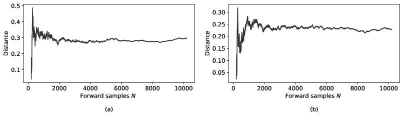
G.4 Bivariate air quality
In Figure 15 we show the posterior mean and standard deviation of the density obtained for the DPMM with MCMC, which is comparable to that of the martingale posterior from the copula method.
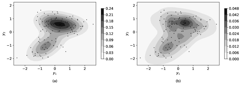
G.5 Classification in simulated moon dataset
We demonstrate the conditional method of Section 4.4.2 with the beta-Bernoulli copula update for classification on a non-linear classification example, which is particularly interesting as we can predictively resample directly. We analyze the simulated moon dataset from sklearn (Pedregosa et al.,, 2011) with bivariate covariates. Figure 16 shows the decision boundary on the left, and simulated data points on the right with a fit GP using the logistic link and Laplace approximation. We fit the conditional copula method and get the bandwidths ; optimizing, fitting and prediction on the -grid of size required 2 seconds, versus around 1 second for the GP.
Predictive resampling is also possible here, where we draw with the Bayesian bootstrap and simulate directly. Generating samples of and computing each on the grid took under seconds. The martingale posterior mean and standard deviations of are shown in Figure 17. The martingale posterior mean is similar to the GP, and we see that the uncertainty is higher in -regions where both classes are present. However, we must note that the uncertainty decreases to 0 as we move away from the data which is undesirable. This may be due to the Bayesian bootstrap resampling from the observed , so in the tails are never sampled. As a result, remains small for in the tails, so there is not much change in . This behaviour is also observed in the conditional copula regression case in Appendix G.6. As such, we recommend only looking at inlying when using the Bayesian bootstrap for with the conditional copula method. On the left of Figure 18, we also plot the martingale posterior of , which has mean but has relatively large uncertainty. On the right, we plot the absolute difference as we carry out one forward sample, which converges relatively quickly with .
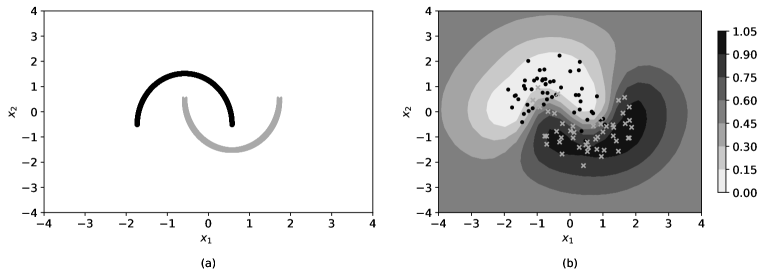

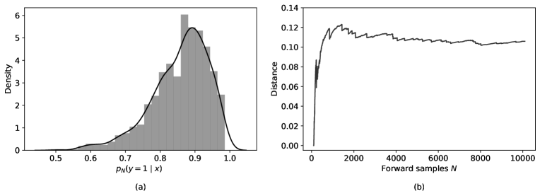
G.6 LIDAR
In Figure 19, we see the predictive means and 95% central intervals for the conditional copula method on the left and the GP on the right. The conditional copula method still performs well, with a slight bias towards the end of range of , in a similar way to the Nadaraya-Watson estimator. The GP deals well with the nonlinearity but much more poorly with the heteroscedasticity.
In Figures 20, 21 we see the difference in the martingale posteriors of for the joint and conditional copula method. For which lies within the data, the uncertainty for the joint and conditional methods are similar. However, for which is far from the data, we see that the joint method has a high amount of uncertainty as expected, but the conditional method does not have any uncertainty. We believe this occurs due to the discrete nature of the Bayesian bootstrap when resampling for the conditional method as discussed in Section G.5. This issue can be mitigated by resampling using a smooth density (e.g. a KDE) for , but still occurs for suitably distant . It seems that the choice of resampling distribution of affects the uncertainty of outlying , but we have found much less sensitivity to this choice for inlying . Interestingly, the joint method does not have this issue irrespective of the distance of from the dataset, so we recommend the joint method when the of interest is outlying. We leave a detailed investigation of this for future work.
We can also see the difference in between the joint and conditional method by comparing Figures 19 and 10. Although the joint method is not skewed towards the end of the range of , the prequential log-likelihood is actually higher for the conditional method. The conditional method is only slightly faster in this example, but for higher dimensional covariates, the computational gain of not having to estimate is much higher. For the median plot in Figure 13(a) in the main paper, we compute the grid of size using the 95% credible bands as the limits for . The median is then computed numerically from the grid where .
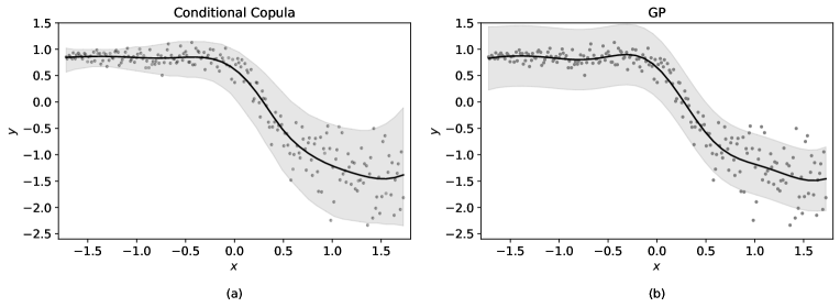
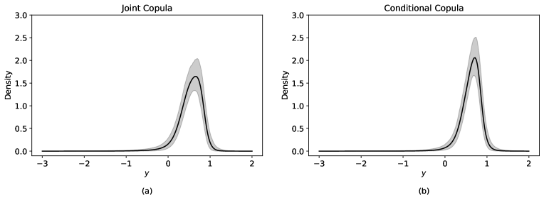
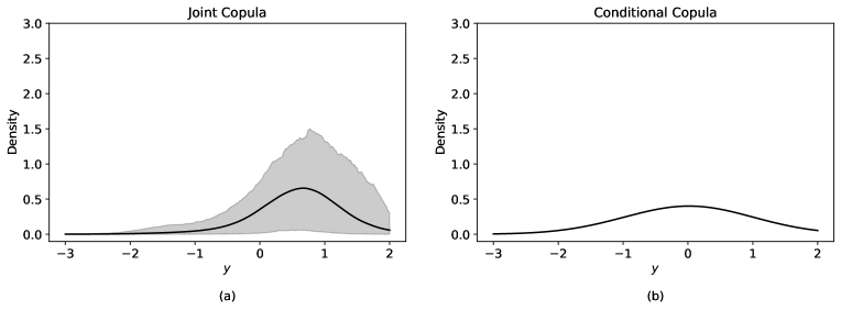
G.7 High-dimensional GMM
In this section, we consider a simulated example to demonstrate the degradation in performance with dimensionality for the DPMM with VI (with diagonal covariance matrix), which the copula method is robust to. We simulate data points from
where and are both -vectors, and is the identity matrix. The DPMM is thus well-specified in this example. As before, we normalize the data before fitting the methods.
Below is a plot of the average test log-likelihoods as increases for each method. The DPMM with VI degrades steeply with dimensionality, likely due to the difficulty of the variational optimization. The KDE performs quite well in this simple example.