Quantum Gravity in Species Regime

Abstract

A large number of particle species allows to formulate quantum gravity in a special double-scaling limit, the species limit. In this regime, quantum gravitational amplitudes simplify substantially. An infinite set of perturbative corrections, that usually blur the picture, vanishes, whereas the collective and non-perturbative effects can be cleanly extracted. Such are the effects that control physics of black holes and of de Sitter and their entanglement curves. In string theory example, we show that the entropy of open strings matches the Gibbons-Hawking entropy of a would-be de Sitter state at the point of saturation of the species bound. This shows, from yet another angle, why quantum gravity/string theory cannot tolerate a de Sitter vacuum. Finally, we discuss various observational implications.

I Introduction and Summary

The main technical obstacle in understanding the microscopic physics of objects such as a black hole or a de Sitter space, is a presumed complexity of quantum gravitational amplitudes in non-perturbative regimes. It is a common perception that processes associated with non-perturbative objects, at weak coupling $\alpha$, are exponentially suppressed ${\rm e}^{-1/\alpha}$.

From here, one is tempted to makes two conclusions. First, non-perturbative effects are completely dwarfed by a variety of contributions that are power-law in $\alpha$. Secondly, at weak coupling, the non-perturbative objects, for all practical purposes, can be treated semi-classically.

However, in several instances the situation is much more subtle. This is the case for the states such as a black hole or a de Sitter Dvali:2011aa ; Dvali:2012en ; Dvali:2013eja ; Dvali:2014gua ; Dvali:2017eba . The reason is that both states belong to the category of the saturated systems, or saturons for short Dvali:2020wqi . Such systems, despite being non-perturbative and macroscopic, depart from semi-classicality rather fast.

For understanding the meaning of saturation, let us first note that non-perturbative processes can be strongly enhanced by the following three factors:

• The occupation number of quanta, $N$;

• The micro-state entropy, $S$;

• The number of interacting particle species, $N_{\rm sp}$.

In fact, the enhancement can be so strong that a given process can be pushed to saturating the unitarity bound. The phenomenon is not limited to gravity and is a generic property of saturons.

I.1 Saturons

This term describes the systems that satisfy the following limiting relation, imposed by unitarity, Dvali:2020wqi :

$$N=\frac{1}{\alpha}=S\,.$$ (1)

Here, $\alpha$ must be understood as the scale-dependent quantum coupling of the theory, evaluated at the size of the system, $R$. As usual, the entropy $S$ is defined as the log from the number of degenerate micro-states.

The saturation condition (1) encodes three relations. The primary idea Dvali:2020wqi ; Dvali:2019jjw is that, for an arbitrary system at weak coupling, unitarity imposes the following upper bound on the entropy,

$$S\leqslant\frac{1}{\alpha}\,.$$ (2)

Correspondingly, a self-sustained system with $N$ constituent quanta, at its maximal entropy capacity, satisfies the relation (1).

It was also argued in Dvali:2020wqi ; Dvali:2019jjw that for a self-sustained system, satisfying (1), the entropy $S$ is equal to the area measured in units of a Goldstone decay constant, $f$. The presence of a Goldstone is generic, due to a spontaneous breaking of Poincare symmetry by any saturon. Thus, the saturation relation (1), also implies the area-form of the entropy,

$$S={\rm Area}\cdot f^{2}=(Rf)^{2}\,.$$ (3)

For definiteness, we wrote the expression in four space-time dimensions, but the same area-law holds in arbitrary dimensions.

Notice, in case of a black hole, the Goldstone of a spontaneously broken Poincare symmetry, is the graviton mode. Its decay constant is a Planck mass $f=M_{P}$. This, was argued in Dvali:2020wqi ; Dvali:2019jjw , shows that the area-form of the Bekenstein-Hawking entropy Bekenstein:1973ur ,

$$S=(RM_{P})^{2}\,,$$ (4)

is a particular example of the area-form of the entropy (3), originating from the phenomenon of saturation. The same is true about Gibbons-Hawking entropy Gibbons:1977mu of de Sitter. This entropy is also given by (4), with $R$ understood as the de Sitter curvature radius.

That is, both, a black hole and a de Sitter Hubble patch, are saturons, as they satisfy (1) and (3). However, the above correlations appear to be universal and to go well beyond gravity Dvali:2020wqi ; Dvali:2019jjw . The meaning of the expressions (1) and (3), shall become more transparent later.

The goal of the present paper is to focus on the role of the third item, the number of particle species $N_{\rm sp}$. Throughout the paper, unless otherwise stated, species will be assumed to be lighter that the relevant energy scale in a given process. We shall primarily be interested in the species of low spin, although most of the results will be applicable in the presence of spin-$2$ species, as it is the case in Kaluza-Klein theories.

The idea is to use the magnifying power of particle species Dvali:2007hz , for cleanly extracting certain quantum gravitational effects. We then apply this method to gravitational saturons in form of black holes and de Sitter.

I.2 Species Limit

We shall define a double-scaling limit in which the Planck mass $M_{P}$ and the number of species $N_{\rm sp}$ are taken infinite while the following relation among them is maintained:

$$M_{P}\rightarrow\infty,~{}N_{\rm sp}\rightarrow\infty\,,~{}\frac{M_{P}}{\sqrt{N_{\rm sp}}}={\rm finite}\,.$$ (5)

This regime has to be supplemented by a proper scaling of the graviton occupation number $N$. We shall refer to (5), as the species limit.

The significance of the species limit (5), from quantum gravitational perspective, is immediately captured by the fact that in this limit the half-decay time of a black hole,

$$t_{\rm half}=R^{3}\frac{M_{P}^{2}}{N_{\rm sp}}\,,$$ (6)

is finite, despite the fact that the black hole mass is infinite. The microscopic meaning of this phenomenon, shall be discussed in details.

In the species regime (5), the quantum gravitational amplitudes simplify significantly. The secondary processes vanish while the non-perturbative effects of interest stay finite. In other words, the species limit (5), allows to distill a set of essential quantum gravitational effects. Some aspects of this extraction were already studied in Dvali:2020wqi ; Dvali:2020etd , on which we shall expand.

Next, we shall apply this treatment to saturons in gravity. As already said, such are black holes and de Sitter. The fact that these states represent saturons, follows from the $S$-matrix formulation of quantum gravity/string theory. In this formulation, both objects must be considered as excited composite states constructed on top of a valid $S$-matrix vacuum, such as Minkowski. In other words, the $S$-matrix formulation leads to their corpuscular resolution.

The corpuscular picture Dvali:2011aa ; Dvali:2012en ; Dvali:2013eja , reveals that black holes as well as de Sitter satisfy the saturation relation (1). Due to saturation, despite of their non-perturbative nature, both systems are susceptible to quantum gravitational effects that alter their semi-classical properties on rather short time-scales. The relevant time-scales are only power-law (or even logarithmic Dvali:2013vxa ) in $1/\alpha$.

I.3 Inner Entanglement and Quantum Break-Time

A particularly important time-scale, delivered by the corpuscular picture, is the quantum break-time $t_{Q}$. The concept was introduced in Dvali:2013vxa , within a prototype model for a black hole $N$-portrait Dvali:2011aa ; Dvali:2012en . It was applied to de Sitter and to black holes in Dvali:2013eja and in subsequent papers. The physical meaning of $t_{Q}$ is that, beyond it, a total breakdown of the semi-classical approximation takes place. The major mechanisms contributing into this departure are: 1) Inner entanglement Dvali:2013eja ; Dvali:2014gua ; Dvali:2017eba ; and 2) Memory burden effect Dvali:2018xpy ; Dvali:2018ytn ; Dvali:2020wft . Both effects shall be reviewed in due course.

As discussed originally in Dvali:2013eja , the above effect is fundamental for understanding physics behind the so-called Page’s curve Page:1993wv . According to Page, the entanglement must reach the maximum after a black hole emits about half of its mass. The semi-classical picture cannot explain this. This picture is blind to an inner structure of the black hole. Because of this, the semi-classical theory captures only one sort of entanglement: The entanglement between a black hole and an outgoing radiation.

The corpuscular picture reveals the existence of another type of entanglement, which we can refer to as the inner entanglement Dvali:2013eja . This effect describes the entanglement among the internal degrees of freedom composing a black hole. Together with the memory burden effect Dvali:2018xpy ; Dvali:2018ytn ; Dvali:2020wft , the inner entanglement grows in time and reaches the maximum, latest, by a half-decay. This is the origin of the quantum break-time $t_{Q}$. These effects offer a new physical meaning for the Page’s curve.

Note, by providing an internal quantum clock, the corpuscular picture predicts the existence of the entanglement curve also for de Sitter Dvali:2013eja . It shows that the entanglement must reach its maximum at the quantum breaking point. In this sense, de Sitter is similar to a black hole. However, beyond $t_{Q}$, the time evolutions of a black hole and of de Sitter exhibit drastic differences. While a black hole can continue its existence beyond $t_{Q}$, for de Sitter this is deadly. The incompatibility of a de Sitter vacuum with the $S$-matrix formulation of quantum gravity, manifests itself though the anomalous quantum break-time Dvali:2020etd .

In the present paper, we shall re-analyse the above dynamics, by taking into account the effect of species. It has already been shown previously that, with other parameters fixed, the species shorten $t_{Q}$. More precisely, for a generic saturated system, $t_{Q}$ scales as Dvali:2017eba ; Dvali:2020wqi ; Dvali:2020etd ,

$$t_{Q}\,=\,\frac{R}{\alpha N_{\rm sp}}\,.$$ (7)

Notice, for a black hole or a de Sitter, this time-scale is equal to (6).

In the present case, we shall study the species effect in various double-scaling regimes, such as (5). This allows us to isolate the three important time scales of: 1) Half-decay; 2) Inner entanglement; 3) Memory burden. All three time-scales are bounded by $t_{Q}$ (7) (and by $t_{\rm half}$ (6)) and remain finite in the species limit (5).

I.4 String Theory

Next, we use the species limit (5) for monitoring the resistance of string theory against the deformation towards a de Sitter state. We take this limit in an explicit string theoretic example in which $n$ $D-\bar{D}$-brane pairs are plied up on top of each other. In the species limit, the string coupling $g_{s}$ vanishes while the number $N_{\rm sp}=n^{2}$ of Chan-Paton factors is taken infinite. At the same time, the product $ng_{s}$ is kept finite. As already shown in Dvali:2020etd , this product determines the quantum break-time $t_{Q}$ of a would-be de Sitter state. Using $ng_{s}$ as a control parameter, we can change $t_{Q}$.

This example reveals some interesting correlations. The entropy of open string modes, matches the Gibbons-Hawking entropy of de Sitter space, when the number of Chan-Paton species saturates the unitarity bound (2). This bound, in the present case reads as, $ng_{s}\lesssim 1$.

At the same point, the thermal corrections from Gibbons-Hawking excitations of the open strings can flip the sign of the tachyon mass and stabilize it. However, for the same values of the parameters, the de Sitter curvature approaches the string scale. Simultaneously, the quantum break-time becomes of order the string length. This is the way the string theory responds to its deformation towards a would-be de Sitter state.

We see that string theory possesses the resources, in form of open string modes, for accounting for Gibbons-Hawking entropy. However, the very same degrees of freedom, speed-up the quantum breaking of the de Sitter “vacuum”. In this way, the string theory exhibits a built-in mechanism restoring the $S$-matrix consistency by abolishing de Sitter.

Finally, we discuss some observational imprints of quantum gravity coming from inflation and from black holes. By consistency, the duration of inflation is bounded from above by $t_{Q}$. Since species shorten $t_{Q}$, they strengthen the quantum gravitational imprints from the inflationary phase, making them potentially-observable, or possibly dominant Dvali:2020etd .

Witten has introduced the concept of meta-observables in de Sitter Witten:2001kn . This concept is linked with the classical no-hair properties of de Sitter. However, the finiteness of $t_{Q}$, effectively can promote them into quantum-observables. Basically, we are saying that $t_{Q}$ endows de Sitter with a quantum hair Dvali:2013eja ; Dvali:2018ytn . This hair is suppressed by $1/t_{Q}$ and so are its observable imprints. Since the species shorten $t_{Q}$ (see, (7)), these imprints can be significant, even for non-far-future observations, if the number of species is high Dvali:2020etd . This magnifying power, is demonstrated by the species limit (5). In this limit, the de Sitter quantum hair is non-vanishing, even though the Planck mass is infinite.

II Species and Scale of Quantum Gravity

The fundamental property of species is the enhancement of the quantum gravitational effects. This phenomenon is linked with lowering the gravitational cutoff, $M_{*}$, by species. Here, the cutoff $M_{*}$ is defined as the scale at which the quantum gravitational interaction becomes strong. In particular, a particle scattering process with momentum-transfer exceeding $M_{*}$, cannot be described within the low energy QFT of gravity. Correspondingly, no semi-classical treatment is possible for such systems. In particular, this concerns the would-be cosmological scenarios with either temperatures or curvatures exceeding the scale $M_{*}$.

The scale $M_{*}$ is highly sensitive to the number of species $N_{\rm sp}$. This follows from the arguments that are independent of perturbation theory. In particular, the black hole physics tells us Dvali:2007hz that in theory with $N_{\rm sp}$ particle species in $4$-dimensions, there is the following upper bound on the scale $M_{*}$,

$$M_{*}=\frac{M_{P}}{\sqrt{N_{\rm sp}}}\,.$$ (8)

Correspondingly, in $d$ space-time dimensions the bound reads,

$$M_{*}=\frac{M_{d}}{N_{\rm sp}^{\frac{1}{d-2}}}\,,$$ (9)

where $M_{d}$ is a $d$-dimensional Planck mass. This bound is non-perturbative and cannot be removed by re-summation. One can arrive to it in several alternative ways. Correspondingly, the bound (8) can be given the several different physical meanings.

We shall briefly recount two physical arguments of Dvali:2007hz . More non-perturbative evidence supporting (8), shall emerge later. The first argument is based on the black hole evaporation. Within the validity of semi-classical gravity, a black hole of mass $M$ and radius $R=M/M_{P}^{2}$, emits a thermal Hawking radiation of temperature $T=1/R=M_{P}^{2}/M$ Hawking:1974sw . Because of its thermal nature and the universality of gravitational interaction, Hawking radiation is democratic in all particle species. Due to this, the mass of a black hole changes in time according to the following Stefan-Boltzmann law,

$$\dot{M}=-N_{\rm sp}T^{2}\,.$$ (10)

Using the relation between the mass and the temperature, we can rewrite this equation in the following form,

$$\frac{\dot{T}}{T^{2}}=N_{\rm sp}\frac{T^{2}}{M_{P}^{2}}\,.$$ (11)

This form is highly instructive. The left hand side of the equation represents a measure of a departure from semi-classicality and thermality. Within the validity of the semi-classical treatment, this quantity must be less than one. This puts an universal upper bound on a temperature of a semi-classical black hole,

$$T_{*}=\frac{M_{P}}{\sqrt{N_{\rm sp}}}\,.$$ (12)

This maximal temperature marks the gravitational cutoff of the low energy theory (8). An extrapolation of the semi-classical regime above this scale, would lead us into an obvious inconsistency. In particular, a black hole of temperature $T\gg T_{*}$, would lose energy faster than its own inverse temperature. Notice, it would radiate its entire mass within the time $\Delta t<1/T\sim R$. This is absurd. Under no circumstances can such a black hole be treated semi-classically.

Alternatively, we can arrive to the bound (8), by considering a maximal possible Gibbons-Hawking temperature of a de Sitter like state in a theory with $N_{\rm sp}$. Since the pioneering work by Gibbons and Hawking Gibbons:1977mu , it is well-known that a de Sitter like Universe (such as an inflationary Universe) is constantly creating particles with thermal-like spectrum of temperature $T_{GH}=H$. Here $H$ is the Hubble parameter, which is related with the de Sitter curvature (Hubble) radius as $H=1/R$. The value of $H$, is determined by the energy density $V$ as, $H^{2}=V/M_{P}^{2}$. In inflation, $V$ is dominated by the potential energy density of the inflaton field.

Similarly to the Hawking radiation of a black hole, within the validity of semi-classical gravity, the Gibbons-Hawking radiation is nearly-thermal. Its energy density is given by,

$$\rho_{GH}=N_{\rm sp}T_{GH}^{4}\,.$$ (13)

It is easy to check that, for a temperature $T_{GH}\gg M_{*}$, this expression would exceed the energy density $V$ of the de Sitter. Of course, this is impossible.

For example, just like in the case of a black hole, a Hubble patch with $H>M_{*}$, would convert its entire energy into the Gibbons-Hawking radiation in less than one Hubble-time, $\Delta t=1/H$. This is again an absurd.

Thus, similarly to the temperature of a black hole (12), $T_{GH}$ is bounded by the scale $M_{*}$ (8). Equivalently, the inflationary Hubble scale is bounded as,

$$H\leqslant\frac{M_{P}}{\sqrt{N_{\rm sp}}}=M_{*}\,.$$ (14)

We shall adopt this as an absolute upper bound. Discussions of other aspects of species bound in de Sitter can be found in Dvali:2008sy .

The bound (8) has also been derived Dvali:2008ec ; Dvali:2008jb ; Brustein:2009ex ; Palti:2019pca from the requirement that a black hole should not exceed the maximal capacity of information storage and processing. In particular, the species entropy should not exceed the standard Bekenstein-Hawking entropy Bekenstein:1973ur of a black hole.

In fact, the information storage capacity is also bounded by the unitarity of the scattering process in which two gravitons, of center of mass energy $E=N_{\rm sp}M_{*}$, produce $N_{\rm sp}$ species Dvali:2020wqi . The unitarity of this process reinforces the bound (2), on the entropy of the final state. This effectively translates as the bound (8). This connection shall be discussed in more details below.

There also exist perturbative arguments supporting (8) (see, e.g., Dvali:2001gx ; Veneziano:2001ah ). We shall limit ourselves with non-perturbative ones, as they cannot be avoided by the re-summation of perturbation series.

III Species Regime of Quantum Gravity

We have seen that non-perturbative arguments unambiguously indicate that quantum gravity is becoming strong at the scale $M_{*}$, given by (8). Already this fact shows that species possess a magnifying power over quantum gravity. Using this power, we would like to cleanly extract certain quantum gravitational effects.

For this, we first define a basic quantum gravitational coupling $\alpha$. Let us consider a tree-level scattering process involving gravitons with momentum-transfer $q$. For example, an annihilation of a pair of gravitons, of a center of mass energy $\sim q$, into a pair of some species. This process is governed by an effective quantum coupling given by

$$\alpha=\frac{q^{2}}{M_{P}^{2}}\,.$$ (15)

This is what we shall call a basic quantum gravitational coupling. In general, in a process with more complicated diagrammatic structure, the coupling $\alpha$ in each vertex is determined by the momentum flow through it.

The momentum-transfer in a graviton vertex shall be restricted by the cutoff $q\leqslant M_{*}$. Correspondingly, the coupling shall satisfy

$$\alpha\leqslant\frac{M_{*}^{2}}{M_{P}^{2}}=\frac{1}{N_{\rm sp}}\,.$$ (16)

In what follows, we shall work in the regime of a weak coupling $\alpha$ and effectively take the limit,

$$\alpha\rightarrow 0\,.$$ (17)

Naively, one may expect that, in this limit, all quantum gravitational effects vanish. However, this is not the case. In reality, (17) allows to make certain phenomena more transparent. For achieving this, the scalings of other quantities must be chosen properly. For the convenience of the description, we shall introduce some useful parameters.

III.1 Species Limit

First, let us define a species coupling,

$$\lambda\equiv N_{\rm sp}\alpha=\frac{q^{2}}{M_{*}^{2}}\,,$$ (18)

where in the very last expression we used the relations (8) and (15).

For a reader familiar with the planar treatment of QCD with large number of colors tHooft:1973alw , it must be clear that the species coupling (18) represents a gravitational analog of ’t Hooft’s coupling. Due to universality of the gravitational interaction, the role of “colors” in gravity is played by the number of all particle species.

This said, there are fundamental differences. Unlike the gluons in QCD, which carry color and anti-color indexes, no species label is carried by the graviton. This suppresses a large number of quantum gravitational processes analogs of which in gluodynamics would be non-zero.

We now take the double-scaling limit (5). In this regime, both $N_{\rm sp}$ and $M_{P}$ become infinite while the scale $M_{*}$ is kept finite. We shall refer to this as the species limit. It is clear from (16) that in this regime $\alpha$ vanishes while $\lambda$ remains finite. The behaviour of various parameters in the species limit is summarized as,

$$M_{P}\rightarrow\infty\,,~{}N_{\rm sp}\rightarrow\infty\,,~{}\alpha\rightarrow 0\,,$$ (19)

$$M_{*}={\rm finite}\,,~{}\lambda={\rm finite}\,.$$

In this regime, the quantum gravity simplifies substantially. All quantum gravitational processes, in which each power of $\alpha$ is not accompanied by $N_{\rm sp}$, vanish. An example is provided by Fig.1a.

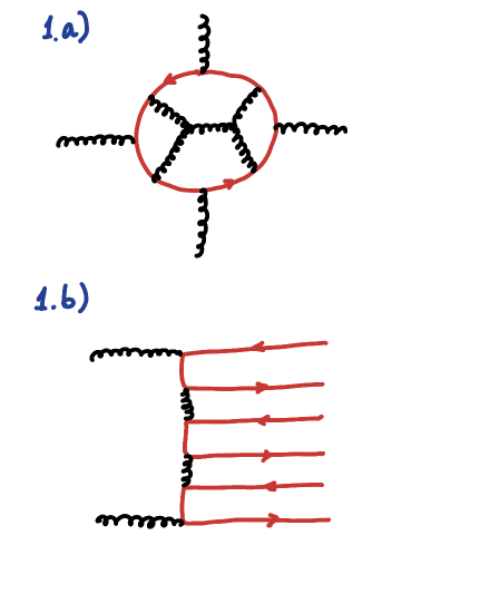
Figure 1: 1.a) An example of a quantum gravitational amplitude that vanishes in the double-scaling limit (19). The gravitons are denotes by black wavy lines and the species by solid red ones. This amplitude scales as $\alpha^{5}N_{\rm sp}=\lambda\alpha^{4}$ and is zero for (19). 1.b) A process of graviton annihilation into $n$ species. For $n\sim N_{\rm sp}$ the cross section is non-zero and for $\lambda\sim 1$ can even saturate unitarity due to a maximal entropy of the final state. It therefore provides an example of a quantum gravitational process that survives in the limit (19).

Let us consider the theory of Einstein gravity, minimally coupled to $N_{\rm sp}$ particle species. We shall treat it as an effective QFT of a graviton ($h_{\mu\nu}$) and of other particle species, formulated on an $S$-matrix vacuum of Minkowski. In such a theory, the linearized metric perturbations are described by excitations of a canonically normalized graviton field around the Minkowski space, $\delta g_{\mu\nu}=\eta_{\mu\nu}+\frac{h_{\mu\nu}}{M_{P}}$. Likewise, the states of arbitrary complexity are viewed as excited states constructed on top of the Minkowski vacuum. For definiteness, we assume that the species are light and stable. We now take the limit (19).

Let us first consider only the states of finite energies. That is, the total energy is allowed to be arbitrarily large, as long as it is finite. Obviously, in such states, the occupation numbers of finite energy (frequency) quanta are also finite.

In such a case, the theory effectively reduces to a linear theory of a massless graviton $h_{\mu\nu}$, coupled to species. The Lagrangian can be written as,

$${\mathcal{L}}=h^{\mu\nu}{\mathcal{E}}_{\mu\nu}\,+\,\frac{1}{M_{*}\sqrt{N_{\rm sp}}}h_{\mu\nu}\sum_{j=1}^{N_{\rm sp}}T_{j}^{\mu\nu}+\,...\,,$$ (20)

where ${\mathcal{E}}_{\mu\nu}$ is the linearized Einstein tensor and $j=1,2,...,N_{\rm sp}$ is the species label. $T_{j}^{\mu\nu}$ are their energy momentum tensors. All the self-couplings of the graviton vanish. The same is true about its couplings to species that are higher than quadratic in $h_{\mu\nu}$.

At the loop level, a relevant correction is a renormalization of the graviton kinetic term by species. In the parameterization of (20), this correction is of zeroth order in $1/N_{\rm sp}$ and, therefore, survives in the species limit (19).

On the other hand, the corrections to non-linear couplings of gravitons vanish. Correspondingly, the same applies to any transition amplitude between finite numbers of initial and final gravitons,

$$N_{in}\rightarrow N_{f}\,.$$ (21)

Such amplitudes are zero to all orders within the validity of $1/N_{\rm sp}$-expansion. An example of a four-loop correction to $2\rightarrow 2$ graviton scattering amplitude, is provided by Fig.1a. This correction scales as $\alpha^{5}N_{\rm sp}=\lambda\alpha^{4}$ and is zero for (19).

Notice, for the suppression of higher order corrections, the relation (8) is of fundamental importance. It is the ability of species, to lower the cutoff relative to $M_{P}$, that enables us to consistently restrict the momentum-transfer among the particles (both, virtual and real) by the scale $M_{*}$. Correspondingly, this restricts the coupling $\alpha$ by $1/N_{\rm sp}$, as indicated by (16).

We also wish to remark that starting with a minimal version of Einstein-Hilbert action, is not essential. We could have instead started with a theory in which infinite series of high order curvature invariants are preemptively added to this action. An each additional derivative would be accompanied by the factor $1/M_{*}$. After canonically normalizing the fields, an $n$-graviton interaction vertex is suppressed by $1/M_{P}^{n-2}$. Due to this, the expansion in terms of the curvature invariants, would effectively be converted into a $1/\sqrt{N_{\rm sp}}$-expansion in terms of graviton interactions. Consequently, all nonlinear self-interactions of graviton would again vanish in the species limit (19).

The simplification of quantum gravity in the species regime (19), allows us to extract non-perturbative processes. As already pointed out in Dvali:2020wqi , in this limit certain collective processes are magnified to the level of saturating unitarity. One example considered there is the process,

$${\rm graviton+graviton}~{}\rightarrow~{}N-{\rm particles}\,,$$ (22)

in which two gravitons, of center of mass energy $E=Nq$, annihilate in $N$ quanta of various species . An each final particle, carries the energy $q$, which is a $1/N$-fraction of the initial energy. A particular diagram contributing to such a process is given by Fig.1b. The amplitude of this process is proportional to $\alpha^{N/2}$ where the effective coupling $\alpha$ is given by (15). Thus, it is of order $N/2$ in $\alpha$-expansion.

The saturation regime is established when the occupation number in the final state is $N=1/\alpha$ while $N_{\rm sp}$ approaches the same value from below. Starting from $\lambda\ll 1$ ($N_{\rm sp}\ll N$), we can scan the process by gradually increasing $\lambda$, keeping other parameters fixed, until it saturates unitarity.

Usually, such a process would be expected to exhibit an exponential suppression, ${\rm e}^{-\frac{1}{\alpha}}$, characteristic of non-perturbative amplitudes. And indeed, it would, if the number of species were small. But, in the present case the story is different. For (19), the transition probability is enhanced by the exponentially large number of possible final states, since the quanta can come from various combinations of species.

This multiplicity can be quantified by the entropy $S$, which can be expressed as a function of $\alpha$ and $\lambda$. Its generic form is,

$$S=\frac{1}{\alpha}\ln(f(\lambda))\,,$$ (23)

where $f(\lambda)$ is a function of $\lambda$. It satisfies $f(\lambda)={\rm e}$ for a certain critical value $\lambda=\lambda_{*}$, typically order one. The precise form of the function $f(\lambda)$ is representation-dependent and is unimportant for the present discussion. For the intuitive usefulness, we just say that its typical form is

$$f(\lambda)=(1+1/\lambda)^{c_{1}\lambda}(1+\lambda)^{c_{2}}{\rm e}^{-c_{3}}\,,$$ (24)

where $c_{1},c_{2},c_{3}$ are positive numbers of order one. More explicit forms can be found in Dvali:2020wqi .

Now, near the saturation point, the cross section (measured in units of $1/q$) takes the form

$$\sigma={\rm e}^{-\frac{1}{\alpha}+S}\,.$$ (25)

Notice that, thanks to the limit (19), the saturation point is insensitive to a non-exponential pre-factor which, therefore, can be set equal to one. The error committed in this way is of order $\alpha$ and vanishes in the limit (19).

From (25) it is clear that the saturation takes place for

$$S=\frac{1}{\alpha}\,.$$ (26)

As already said, this is reached for $\lambda=\lambda_{*}\sim 1$. It is clear that at this point, the final state of species satisfies a saturon relation (1). Notice, for $q=M_{*}$, the unitarity of the process bounds $N_{\rm sp}$ exactly by (8). This gives an alternative derivation of the species bound on $M_{*}$ from saturation.

III.2 Collective Limit

We have seen that the species limit (19) allows to cleanly extract a set of non-perturbative processes. This is possible, despite the fact that the gravitational coupling $\alpha$ vanishes. In the considered process, the suppression is compensated by the number of species and the corresponding entropy of the state. We shall now turn to a different class of quantum gravitational processes that survive in the species limit (19). These are the transitions that are enhanced by the occupation number of gravitons, $N$.

In such cases, an interaction vertex of gravitons that vanishes in the limit (19), can nevertheless generate a non-trivial transition. For example, a $2\rightarrow 2$ transition amplitude, caused by a tree-level four-graviton vertex, is suppressed by $\alpha$. Nevertheless, the transition matrix element can be non-zero in the limit (19), provided the occupation number of quanta scales as,

$$N\propto\frac{1}{\alpha}\,.$$ (27)

In order to account for such cases, it is convenient to introduce the notion of the collective coupling, defined as,

$$\lambda_{c}\equiv N\alpha\,.$$ (28)

Originally, this concept was introduced in the context of the black hole $N$-portrait.

It is important not to confuse the occupation number of gravitons $N$ in a state, with the number of species $N_{\rm sp}$ in the theory. Correspondingly, we should not confuse the collective coupling $\lambda_{c}$, with the species coupling $\lambda$ defined in (18). The species coupling $\lambda$, is a parameter of the theory, since it depends on $N_{\rm sp}$. In contrast, the collective coupling $\lambda_{c}$, is a parameter of the state, which depends on the occupation number $N$ in that state.

The concept of collective coupling, allows us to define the second double-scaling limit,

$$M_{P}\rightarrow\infty\,,~{}N\rightarrow\infty\,,~{}\alpha\rightarrow 0\,,$$ (29)

$$\lambda_{c}={\rm finite}\,,~{}N_{\rm sp}={\rm finite}\,.$$

We shall refer to it as the collective limit. This limit requires some clarification. Since we kept $N_{\rm sp}$ finite, the fixed hierarchy between the cutoff $M_{*}$ and $M_{P}$ is maintained. In such a case, setting $\alpha$ to zero implies a restriction on $q$, for example, by considering a tree-level process with a finite momentum transfer among gravitons. Such restrictions need not be obeyed by the virtual quanta. As a result, the corrections from UV-sensitive loops, translate as $1/N_{\rm sp}$-corrections. This is different from the species regime (19), in which the analpogous corrections vanish.

Obviously, in the regime (29), the species coupling $\lambda$ vanishes together with $\alpha$. Because of this, we may expect that quantum gravity becomes trivial in IR Brustein:2009ex . However, this expectation does not capture the collective effects that are enhanced by $N$.

Naturally, those processes that are controlled by the collective coupling $\lambda_{c}$, are non-zero in the limit (29). For example, we choose an initial state $\left|\,N\right>$, in which gravitons of certain wavelength $R$ are macroscopically occupied, so that $\lambda_{c}$ is non-zero. Let us consider a process, in which two initial gravitons re-scatter into a pair of final gravitons, as it is sketched in Fig.2b. Alternatively, the same pair can annihilate into a pair of species, as described by Fig.2a. The matrix elements of both transitions are proportional to $\lambda_{c}$. Correspondingly, they are both non-vanishing in the collective limit (29). At the same time, all the higher order corrections in $\alpha$, not accompanied by the corresponding powers of $N$, vanish.

The processes of the sort of Fig.2, can have a wide range of physical applications. In particular, they describe the processes of the gravitational particle-creation by black holes and by de Sitter in the corpuscular theory of Dvali:2011aa ; Dvali:2013eja .

The sketch in Fig.2b, also reveals why the self-binding potential of $N$ overlapping gravitons, survives in the collective limit (29). This diagram describes the origin of the attractive potential, at the level of a virtual one-graviton exchange among the real gravitons. The attractive potential energy, experienced by each graviton from its $N$ neighbours, is $E_{\rm pot}\sim\lambda_{c}/R$. For $\lambda_{c}\sim 1$, this potential can balance the kinetic energy of a would-be free graviton ($E_{\rm kin}\sim 1/R$). At this point, $N$ gravitons form a self-sustained bound-state. This bound-state represents a corpuscular description of a black hole Dvali:2011aa ; Dvali:2012en ; Dvali:2013eja .

III.3 Species Magnifier Limit

Finally, we shall discuss a regime, which is of special interest for our applications. This regime was previously introduced in Dvali:2020wqi and we shall refer to it as the limit of species magnifier. It has the following form,

$$\alpha\rightarrow 0\,,~{}N\rightarrow\infty\,,~{}N_{\rm sp}\rightarrow\infty\,,$$

$$M_{*}={\rm finite}\,,~{}\lambda={\rm finite}\,,~{}\lambda_{c}={\rm finite}\,.$$

Basically, the above limit describes the species regime (19), in the presence of a state with infinite occupation number $N$ of gravitons, such that the ratio $N/N_{\rm sp}$ is finite.

Correspondingly, while this regime maintains benefits of the species limit (19), it enables to expose non-trivial collective phenomena. For example, a four-graviton interaction vertex can trigger a non-trivial transition from an initial $N$-graviton state via a re-scattering of two constituents. The matrix element of this process is controlled by $\lambda_{c}$. At the same time, the loop corrections to the same vertex, such as Fig.1a, vanish.

In order to capture more essence of the limit (III.3), let us compare the outcomes of the process of Fig.2a in the regimes (29) and (III.3). As already mentioned, this process describes the scattering of two gravitons into an arbitrary pair of species. The rate of this process is enhanced by $N_{\rm sp}$ due to the number of available final states. It scales as,

$$\Gamma\sim q\lambda_{c}^{2}N_{\rm sp}\,,$$ (31)

where $q=1/R$ is a characteristic energy of the initial gravitons. The inverse of this rate, gives the time-scale during which the number of initial gravitons is reduced roughly by two. Of course, there are other processes that contribute but this one suffices for making the point.

As a reference unit of time, we can adopt $R=1/q$. During this time, the relative reduction of the graviton number is,

$$\frac{\Delta N}{N}\sim\frac{N_{\rm sp}}{N}\,\lambda_{c}^{2}\,.$$ (32)

This quantity represents a measure of the quantum gravitational back reaction on the state.

Correspondingly, the time-scale $t_{\rm half}$, during which the initial state would loose roughly half of its constituents, is given by,

$$t_{\rm half}\sim\frac{R}{\lambda_{c}^{2}}\frac{N}{N_{\rm sp}}\,.$$ (33)

We shall now compare the behaviour of the above three quantities (31)-(32)-(33), in the two different regimes of (29) and (III.3).

We start with the collective limit (29). In this regime, the emission rate (31) is finite. However, the quantum gravitational back reaction (32) is zero. Correspondingly, the half-decay time (III.3) is infinite. The physical reason behind this behaviour is no secret. In the collective limit (29), the initial graviton occupation number $N$, is infinite. Such a state behaves as a graviton reservoir of infinite capacity. A finite depletion rate, is not capable of destroying such a system within any finite time. In other words, the fraction of gravitons depleted within any finite interval of time, is of measure-zero. This explains why the back reaction (32) is vanishing.

In the species magnifier regime (III.3), the situation changes drastically. The infinite number of species $N_{\rm sp}$, opens up an infinite number of the decay channels. Correspondingly, the rate (31) blows up. However, the problem is regular. The back-reaction (32) is finite and so is the half-decay time (33) of the graviton condensate.

The important aspect of the magnifier limit is that it captures the quantum gravitational back-reaction, despite the fact that $\alpha=0$. At the same time, the secondary effects, that are higher order in $\alpha$, vanish.

To summarize, working in the regime (III.3) provides us with a double advantage. First, it allows to cleanly distill some collective and non-perturbative quantum gravitational phenomena. Secondly, it shows that, for large $N_{\rm sp}$, the quantum gravity can leave significant imprints at distances much larger than the Planck length. The species literally act as a “magnifying glass” for quantum gravity.

In what follows, we shall apply the species regime for extracting certain quantum gravitational effects in de Sitter and in black holes and for understanding their observational implications.

IV Corpuscular Theory

IV.1 Motivation

As we have seen, the magnifying effect of species can be deduced already within the semi-classical treatment. The relations such as (8), do not require the knowledge of an internal corpuscular structure of either a black hole or a de Sitter. The semi-classical picture is of course incomplete. Although this picture allows to derive the species bound (8), it cannot grasp the fundamental physics behind it. For example, it is not clear, how a back-reaction from particle-creation, affects a black hole or a de Sitter.

In order to answer the next layer of questions, we must work within a more fundamental framework, in which the corpuscular structure is visible. Once we have such a picture, we shall supplement it with a large number of light particle species. This shall enable us to work in the regime (III.3) and to use species as a magnifying tool.

The corpuscular picture we shall work with, is the quantum $N$-portrait Dvali:2011aa ; Dvali:2012en ; Dvali:2013eja . In this picture, a black hole or a de Sitter Hubble patch, is described as a composite state of soft gravitons of mean occupation number $N$. This state satisfies the saturation relation (1).

A particularly strong motivation for the corpuscular picture, is provided by the $S$-matrix formulation of quantum gravity. This formulation demands the existence of a valid $S$-matrix vacuum. All other states, must be described as excited states, constructed on top of this vacuum.

The de Sitter cannot serve as a valid $S$-matrix vacuum for quantum gravity. The absence of a globally-defined time, is part of the problem. However, the issue is more subtle and is linked with the very nature of quantum gravity/string theory Dvali:2020etd . The point is that, in general, a valid vacuum must not recoil and absorb information in a scattering process. A de Sitter can satisfy this requirement, but exclusively in the following double scaling limit,

$$M_{P}\rightarrow\infty,~{}R={\rm finite}\,.$$ (34)

In this limit, the quantum graviton coupling (15), vanishes. Hence, whenever de Sitter becomes a rigid vacuum, gravitons (closed strings) decouple. In other words, de Sitter can be promoted into a “vacuum” only at the expense of trivializing the graviton (closed string) $S$-matrix. Notice, at the same time, non-gravitational interactions can remain non-trivial for (34). In particular, for interactions that are asymptotically-free, an approximate $S$-matrix treatment becomes better and better at short distances and can be consistently formulated in the limit (34).

The important message we take from this analysis, is that the $S$-matrix formulation excludes a de Sitter vacuum for any finite value of $M_{P}$. The only remaining option is to treat de Sitter as an excited (coherent) state constructed on top of a valid $S$-matrix vacuum such as Minkowski Dvali:2011aa ; Dvali:2013eja ; Dvali:2014gua ; Dvali:2017eba . Various other aspects of this idea have been discussed Kuhnel:2014gja ; Kuhnel:2015yka ; Casadio:2015xva ; Berezhiani:2016grw , including string context Brahma:2020htg .

The $S$-matrix justification for the corpuscular structure of a black hole Dvali:2011aa , is more straightforward. There is a little doubt that a black hole of size $R$, can be produced in an $S$-matrix process of center of mass energy $E\sim M_{P}^{2}R$ tHooft:1987vrq ; Amati:1987wq ; Gross:1987kza . The new insight, brought by the corpuscular $N$-portrait Dvali:2011aa is the identification of the relevant $S$-matrix process in form of $2\rightarrow N$ graviton scattering, where the occupation number of the final gravitons is $N\sim(RM_{P})^{2}$ and their wavelengths are $\sim R$. It has been observed Dvali:2014ila ; Addazi:2016ksu that such a $2\rightarrow N$ graviton scattering process, saturates unitarity precisely when the entropy of the final state matches the Bekenstein-Hawking entropy of a black hole of size $R$. It is therefore natural to describe a black hole as a “loose” bound-state of $N$ such quanta. This justifies the idea of the black hole $N$-portrait, from the $S$-matrix perspective.

IV.2 Two Types of Constituents

The corpuscular pictures for a black hole and for de Sitter exhibit close similarities. Therefore, we shall discuss them in a common language. This language also allows to grasp the fundamental differences between the two systems. These differences, become important at the later stages of their time-evolutions.

In both cases, the relevant gravitational radius shall be denoted by $R$. In classical theory, this scale describes a Hubble radius ($R=1/H$) for de Sitter and a Schwarzschild radius for a black hole.

The constituents are divided in two main categories: The master modes and the memory modes.

The master modes, to be symbolically denoted by creation/annihilation operators $\hat{a}^{\dagger}$/$\hat{a}$, are the main contributors into the energy of the system (a black hole or a Hubble patch). The diversity of the master modes is small, but they come in high occupation numbers. Because of this, they contribute predominantly into the energy but very little into the information capacity of the system.

The memory modes, to be denoted by $\hat{b}^{\dagger}$/$\hat{b}$, play the opposite role. They are responsible for the information storage capacity of the system. This capacity is measured by the micro-state entropy $S$. This stands for Bekenstein-Hawking entropy for a black hole and Gibbons-Hawking entropy for de Sitter. The memory modes are initially (nearly) gapless. Due to this, they contribute negligibly into the energy. However, unlike the master modes, the memory modes come in a very large diversity of “flavors”. This is the reason for why they account for the entropy of the system.

We shall briefly review each category.

IV.2.1 Master Modes

The characteristic frequencies (${\mathcal{E}}_{\rm master}$) and wavelengths ($l_{master}$) of the master modes are both set by the scale $R$,

$${\mathcal{E}}_{\rm master}\sim\frac{1}{l_{\rm master}}\sim R\,.$$ (35)

That is, the dispersion relations of the master modes are not too far from the dispersion relations of the free gravitons, propagating on top of the Minkowski vacuum.

This is explained by the self-sustainability condition that was already discussed previously. The attractive potential, experienced by each master graviton, is comparable to its kinetic energy. Therefore, the collective gravitational interaction, while sufficiently strong for holding the master modes together, only mildly modifies their dispersion relations. The essence of this collective interaction was already discussed and illustrated by a sketch in Fig.2b.

The master gravitons are the main contributors into the initial energy of the system. An each quantum contributes roughly $1/R$. The total energy is thus proportional to their occupation number,

$$E=N{\mathcal{E}}_{\rm master}=\frac{N}{R}\,.$$ (36)

Given the standard relation,

$$E=RM_{P}^{2}\,,$$ (37)

between the energy (mass) and a size of a black hole (or a Hubble patch), we get,

$$N=(M_{P}R)^{2}\,.$$ (38)

The basic quantum gravitational coupling of the master gravitons is given by (15) evaluated for $q\sim 1/R$,

$$\alpha=\frac{1}{(RM_{P})^{2}}\,.$$ (39)

This given two important relations. First, for both systems the above expression is equal to the inverse of the entropy $S$ (Bekenstein-Hawking entropy for a black hole and Gibbons-Hawking entropy for de Sitter). Both entropies are equal to (4).

Secondly, the number of constituents $N$ is equal to the inverse of their coupling (and equivalently, to the entropy). Thus, both, a black hole and a de Sitter, satisfy the saturation relation (1). Taking into account the explicit form of the entropy (4), the saturation relation reads as,

$$N=\frac{1}{\alpha}=S=(RM_{P})^{2}\,.$$ (40)

As pointed out in Dvali:2020wqi ; Dvali:2019jjw and also explained earlier in the present paper, the area form of the entropy (4) represents a particular case of the generic property of saturons. The entropy of a saturon is always given by its area measured in units of the decay constant of the Goldstone boson of spontaneously broken Poincare symmetry. The emergence of such a Goldstone boson is generic, because any saturon breaks Poincare symmetry spontaneously. In case of a black hole or a de Sitter, the Goldstone boson in question is the graviton, but the effect is universal and goes beyond gravity (See, Dvali:2020wqi ; Dvali:2019jjw for explicit examples.)

The concept of spontaneous breaking of Poincare symmetry by the saturated $N$-graviton state, is best defined in large-$N$ limit (29). The order parameter of this breaking is $\sqrt{N}/R$, which, by Goldstone theorem, determines the decay constant of a canonically normalized Goldstone mode. As it is clear from (38), this quantity is nothing but the Planck mass, $M_{P}$, which represents the graviton decay constant. This fully matches the fact that the Goldstone boson of Poincare symmetry, originates from the graviton. The above explains why $M_{P}$ enters in the expression (4) for the area-form of the entropy.

The relation (40) indicates that both systems (black hole and de Sitter) represent saturons. This is defining for their physical properties.

IV.2.2 Memory Modes

Unlike the master modes, the memory modes have very short wavelengths (of order the cutoff) but almost zero frequencies. Namely, the energy gap for exciting a memory mode is,

$${\mathcal{E}}_{\rm memory}\sim\frac{1}{NR}\ll\frac{1}{l_{\rm memory}}\,.$$ (41)

Obviously, the dispersion relations of the memory modes are very different from those of free gravitons. A free graviton, of some wavelength $l$, propagating on Minkowski vacuum, would have a frequency, $\sim 1/l$. This is due to the Poincare symmetry of the Minkowski background.

However, the dispersion relations of the memory modes, are affected by the presence of the master modes. As already discussed, the state of $N$ master modes, breaks the Poincare symmetry spontaneously. As a result of this breaking, the dispersion relations of the would-be “hard” memory modes are strongly affected. Their wavelengths stay short, but their frequencies are redshifted to almost zero. In fact, the memory modes become exactly gapless in the collective limit (29). At finite $N$, their gaps scale as (41).

The variety of the “flavors” of the memory modes is of order $1/\alpha$. This is determined by the number of different momentum oscillators that become gapless at the saturation point. Due to this, the memory modes are the main contributors into the entropy of the system. These modes are gapless because of the critical occupation number of the master modes. That is, the energy gaps of the memory modes depend on the occupation number of the master mode. The gaps collapse to (almost) zero when the occupation number of the master mode reaches a critical value.

This phenomenon, schematically, can be described by the following Hamiltonian (see, e.g., Dvali:2017nis ; Dvali:2018xpy ),

$$\hat{H}=\sum_{b}\omega_{b}\left(1-\alpha\,\hat{a}^{\dagger}\hat{a}\right)^{2}\hat{b}^{\dagger}\hat{b}\,.$$ (42)

For simplicity of illustration, we took a single master mode. The summation is over various memory modes. $\omega_{b}$ are their would-be frequencies in the Minkowski vacuum, which typically are very high (of order the cutoff or so).

The reader should not be alarmed by the oversimplified appearance of the above Hamiltonian. In particular, by its number-conserving form. These details are unimportant and have been neglected for making the essence of the phenomenon maximally transparent. Thanks to the power of saturation, the (42) captures this essence surprisingly well. In fact, near the saturation point (40), the dynamics of a generic system effectively reduced to the above, up to a proper Bogoliubov transformation.

In a state with the occupation number of the master mode $\langle\hat{a}^{\dagger}\hat{a}\rangle\equiv N$, the effective energy gaps of the memory modes are given by

$${\mathcal{E}}_{\rm memory}=\omega_{b}\left(1-\alpha N\right)^{2}\,.$$ (43)

It is clear that the memory modes become effectively gapless over a state in which $N$ is critical,

$$N=\frac{1}{\alpha}\,.$$ (44)

Since the memory modes are gapless, an exponentially large number of degenerate micro-states emerges. These states differ by the occupation numbers of the memory modes. This is the reason behind the maximal entropy of the saturated system.

Thus, we can say that in a saturated state the master mode assists Dvali:2018tqi the memory modes in becoming gapless. Away from saturation (40), the memory modes are very costly in energy, but at the saturation point, they cost nothing. Thanks to this phenomenon, the memory modes can store a large amount of information at almost zero energy expense.

Thus, a black hole or a de Sitter state is described by the occupation number of the master mode and the ones of the memory modes. This state can be denoted as,

$$\left|\,N\right>=\left|\,N\right>_{a}\left|\,n_{1},n_{2},...\right>_{b}\,,$$ (45)

where $\left|\,N\right>_{a}$ is a state of a master mode, with occupation number $N$, and $\left|\,n_{1},n_{2},...\right>_{b}$ is a state of memory modes, with various occupation numbers. An each sequence, represents a memory pattern. The number of distinct patterns is exponentially large,

$$n_{st}\sim{\rm e}^{1/\alpha}\,.$$ (46)

As long as the system is saturated (40), the patterns are degenerate in energy (up to $1/N$ corrections). They form a set of micro-states that are classically indistinguishable. The corresponding micro-state entropy is,

$$S=\ln(n_{st})=\frac{1}{\alpha}=(RM_{P})^{2}\,.$$ (47)

This is the origin of Bekenstein-Hawking and Gibbons-Hawking entropies in the corpuscular picture.

As said, the above presentation captures the essence of the story. We needed to display the necessary ingredients of the phenomenon before highlighting the magnifying role of the particle species in it.

IV.3 Saturation

The saturation relation (1) can be written as,

$${\rm Number}=\frac{1}{\rm Coupling}={\rm Entropy}\,.$$ (48)

The saturons (the systems satisfying this relation) exhibit certain universal phenomena. For the present discussion, the most important is the effect of quantum breaking and the internal mechanisms leading to it.

The main engine of the time-evolution of a saturated system, is the re-scattering of the master modes. This re-scattering leads to the processes that are observable on the time-scales $\sim R$. For example, such is a process of particle-emission, which leads to the decay of a saturon.

Since the memory modes have very low frequencies (41), the time-scale of their evolution would be,

$$t_{\rm memory}\sim NR\,.$$ (49)

In addition, the memory modes are affected by the re-scatterings of the master modes, over a similar time-scale.

There exist three important effects contributing into the time-evolution of the saturon state:

• The reduction of the occupation number of the master mode. This is the flip side of the particle emission.

• The inner (or self) entanglement Dvali:2013eja ; Dvali:2014gua ; Dvali:2017eba : The constituents of a black hole (or a de Sitter) become internally entangled among each other.

• The memory burden effect Dvali:2018xpy ; Dvali:2018ytn ; Dvali:2020wft : With the decrease of the occupation number of the master mode, the system departs from saturation. Correspondingly, the gaps of the memory modes grow. This generates a quantum back-reaction force.

All three effects lead to a complete breakdown of the semi-classical picture. This phenomenon is referred to as the quantum breaking. The corresponding time-scale is called a quantum break-time $t_{Q}$. For a de Sitter and a black hole, $t_{Q}$ was derived in Dvali:2013eja ; Dvali:2014gua ; Dvali:2017eba . For a generic saturated system (without classical instability) Dvali:2017eba ; Dvali:2020wqi it is given by (7), which can be presented as,

$$t_{Q}\sim\frac{t_{\rm cl}}{\lambda}\,.$$ (50)

Here, $t_{\rm cl}$ is the classical time-scale set by the frequencies of the constituents, $t_{\rm cl}\sim R$. $\lambda\equiv\alpha N_{\rm sp}$ is the analog of species coupling (18) (’t Hooft coupling), for the generic saturated system.

The various aspects of the above effects have already been studied in saturated gravitational systems, such as black holes and de Sitter. In the present paper we are interested in the magnifying role of species in these processes. For completeness, in parallel, we shall briefly reproduce the essence of the phenomena.

IV.4 Quantum Clock: Re-scattering and Depletion

Initially, the main engine of the time-evolution is the re-scattering of the master modes. The memory modes, since at this stage they are essentially gapless, back react very little and can be ignored. However, back reaction becomes very important at later times.

The initial re-scattering of the master modes, takes place regardless of the number of species in the theory. However, species speed it up. One outcome of this re-scattering, is the emission of free particles. The typical process is depicted in Fig.2a. For a black hole and a de Sitter, the produced particles describe Hawking and Gibbons-Hawking quanta, respectively.

For describing the process, we can use the formulas (31), (32), (33) obtained for a generic $N$-graviton state. The new specifics is that, at initial times, the parameters are related by the saturation relation (40).

The rate of particle-creation is,

$$\Gamma=\frac{1}{R}(N\alpha)^{2}N_{\rm sp}=\frac{1}{R}N\lambda_{c}\lambda\,.$$ (51)

As expected, at initial times, the rate of particle-production, reproduces the semi-classical Hawking and Gibbons-Hawking rates. Note Dvali:2013eja , a particular channel, describing a creation of a graviton, corresponds to the standard tensor perturbation mode of inflation Starobinsky:1979ty .

However, the corpuscular picture allows us to go beyond the semi-classical approximation. Using the microscopic description, it is instructive to consider the physical meaning of particle-creation from different perspectives.

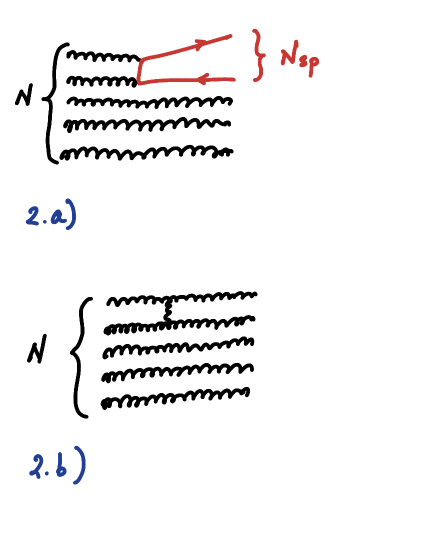
Figure 2: 2.a) Decay of the multi-graviton state into species (red line) illustrates the enhancement of the rate of the process due to high occupation number of the initial state. The suppression factor $\alpha^{2}$ is compensated by multiplicity factor $N^{2}$. 2.b) Illustrates the finiteness of the collective effect, experienced by each graviton due to its interactions with the neighbours.

First, using the saturation relation (40), valid for initial times, we can write the rate (51) in terms of the species coupling,

$$\Gamma_{in}=\frac{1}{R}N_{\rm sp}=\frac{1}{R}\frac{\lambda}{\alpha}\,.$$ (52)

This form, clearly shows the magnifying power of species. As already discussed earlier for a generic $N$-state, in the double-scaling limit (III.3), the rate (51) blows up. However, this blow-up does not lead to any sort of inconsistency. The saturation relation (40) guarantees that, in the same limit, the mass of a black hole (or of a de Sitter Hubble patch), (37), becomes infinite.

As a result, the back-reaction over time $R$ (32), is finite. Due to saturation (40), in the present case, the back-reaction (32) takes the form,

$$\frac{\Delta N}{N}=\frac{N_{\rm sp}}{N}\,.$$ (53)

Correspondingly, the time of half-decay,

$$t_{\rm half}=\frac{R}{\lambda}=\frac{R^{3}M_{P}^{2}}{N_{\rm sp}}=R^{3}M_{*}^{2}\,,$$ (54)

is also finite.

The corpuscular picture makes it very clear that the particles are not produced “for free”. Due to back-reaction, the coherent state depletes and looses coherence. This is true for black holes, as well as, for de Sitter.

The rate of the departure from coherence can be estimated by using the fact that the number of quanta in a coherent superposition diminishes with roughly the same rate (51) as the particles are emitted. That is,

$$\dot{N}=-\Gamma\,.$$ (55)

For estimating the back-reaction, in the leading order, the coupling $\alpha$ can be taken constant. Then, at initial times, the rate of particle-production changes as (as everywhere, unimportant numerical coefficients are set equal to one),

$$\frac{\dot{\Gamma}}{\Gamma} = -\frac{1}{R}N\alpha^{2}N_{\rm sp}=-\frac{1}{R}\lambda_{c}\lambda\,.$$ (56)

Now, approximating the quantities on the right hand side by their initial saturated values (40), we get,

$$\Gamma(t)=\Gamma_{in}{\rm e}^{-\frac{t}{t_{\rm half}}}\,,$$ (57)

where $t_{\rm half}$ is given by (54).

The expressions (51) and (57) are instructive due to several reasons. First, for de Sitter, they reinforce the upper bound (14) on $H$. We see from (51) that the violation of this bound would lead to an unacceptably high rate of depletion. With such a gigantic decay rate, the de Sitter state would cease to exist in less than one Hubble time. In full agreement with this, (57) shows that the production rate would drop in less than one Hubble time.

Similarly Dvali:2012uq , for a black hole this reinforces the upper bound (12) on Hawking temperature. A hotter black hole cannot exist. Such a black hole, would emit all its constituents within the time less than its size. This would make no sense.

To summarize, species produce the two inseparable effects. First, they enhance the rate of particle-production. Secondly, as a result of back-reaction, species speed up an intrinsic quantum clock. This clock measures the depletion of $N$-graviton state which describes a black hole or a de Sitter. The flip side of this process is the generation and growth of entanglement which we shall now discuss.

IV.5 Entanglement and Page’s Curve

The corpuscular picture reveals a new phenomenon, which we can call a self-entanglement or an inner entanglement Dvali:2013eja . This takes place, both for de Sitter and for a black hole. In both cases, the growth of inner entanglement happens at the same rate as the particle emission. Together with the depletion, the self-entanglement contributes into the departure from classicality. It reaches the maximum at quantum break-time Dvali:2013eja ; Dvali:2014gua ; Dvali:2017eba ,

$$t_{Q}=\frac{R^{3}M_{P}^{2}}{N_{\rm sp}}=\frac{R}{\lambda}=R^{3}M_{*}^{2}\,.$$ (58)

It is easy to notice that this is a particular case of (50), applied to a gravitational saturon. The time-scale (58) signals a complete break-down of the semi-classical picture. The quantum break-time has been verified in various contexts Dvali:2017ruz ; Kovtun:2020ndc ; Kovtun:2020kcl ; Berezhiani:2020pbv ; Blumenhagen:2020doa .

From (54) it is clear that $t_{Q}$ matches the time of half-decay, but brings a new physical meaning. The effect is intrinsically corpuscular in nature and cannot be observed in semi-classical theory. This is why, unless additional assumptions are invoked, the behaviour of entanglement in semi-classical treatment is related with certain puzzling features of Page curve. According to Page Page:1993wv , the entanglement must reach a maximal value after $t_{\rm half}$. This is exactly what corpuscular theory predicts. The semi-classical picture cannot explain this.

In semi-classical treatment, the sole engine for the Page’s curve, is the entanglement between the black hole and an outgoing Hawking radiation. This creates a false impression that the entanglement grows indefinitely throughout the black hole existence. However, this picture is incomplete and requires a corpuscular resolution which incorporates the inner entanglement and memory burden effects.

As already shown in Dvali:2013eja , the corpuscular theory immediately accommodates Page’s central point. The entanglement of a saturated $N$-particle state cannot grow indefinitely. It reaches the maximum after the quantum break-time $t_{Q}$. The fact that $t_{Q}$ comes out equal to Page’s time, can be taken as consistency check of the picture.

The corpuscular approach shows that the analog of Page’s time exists also in de Sitter Dvali:2013eja . For both systems, the re-scattering of the constituent gravitons (which also leads to particle emission), generates an internal entanglement among the remaining constituents Dvali:2013eja . Simultaneously, it creates the memory burden effect Dvali:2018xpy in de Sitter Dvali:2018ytn and in black holes Dvali:2020wft .

IV.6 Inner entanglement

After the emission of a single particle, the state (45) evolves into a following superposition,

$$\left|\,N\right>\rightarrow\sum_{j}^{N_{\rm sp}}c_{j}\left|\,N^{\prime},j\right>\times\left|\,j\right>\,,$$ (59)

where $c_{j}$ are constants. Here, $j=1,2,...,N_{\rm sp}$ is the species label that characterizes various states of emitted quanta, which are denoted by $\left|\,j\right>$. Since we are not in a semi-classical picture, the term “emitted quanta” requires a specification. It describes quanta with dispersion relations that are close to quantum particles propagating in a background de Sitter (or Schwarzschild) metric.

Notice, in de Sitter, this is a fine definition at initial times. Later, towards the quantum break time, the classical de Sitter geometry looses the meaning. By then, the distinction between the emitted and retained quanta becomes blurry. However, this is not an issue, since after $t_{Q}$ we are already in a quantum-broken phase. Beyond this point, the de Sitter cannot exist as a valid state. A graceful exit must take place before the time $t_{Q}$ elapses.

In contrast, the black holes can exist beyond $t_{Q}$. Also, for them, the notion of the emitted quantum is well defined at all times.

Of course, at the initial times, the emission is democratic in species, since they are produced via graviton processes. The states $\left|\,N^{\prime},j\right>$ denote what remains from a black hole or a Hubble patch after the emission. The expression (59) shows that these states are entangled with outgoing quanta through the label $\left|\,j\right>$.

The crucial point is that each $\left|\,N^{\prime},j\right>$ is also self-entangled. That is, even if initial $\left|\,N\right>$ was a tensor product state of various master and memory modes, $\left|\,N_{a_{1}}\right>\left|\,N_{a_{2}}\right>...\left|\,n_{b_{1}}\right>\left|\,n_{b_{2}}\right>$, in the state $\left|\,N^{\prime},j\right>$ they become entangled. In other words, the state evolves into a superposition,

$$\left|\,N^{\prime}\right>=\sum_{a,b}c_{a_{1},a_{2},..b_{1},b_{2},...}\left|\,N_{a_{1}}\right>\left|\,N_{a_{2}}\right>...\left|\,n_{b_{1}}\right>\left|\,n_{b_{2}}\right>\,,$$ (60)

where $c_{a_{1},a_{2},..b_{1},b_{2},...}$ are coefficients. We have deliberately ignored the label of the emitted species $j$, in order to focus on the internal entanglement. In addition, of course, the state is entangled with respect to the species index $j$.

Let the number of linearly-independent states participating in the superposition (60) be $\tilde{n}_{\rm st}$. We shall measure the level of the entanglement by the log of this number:

$$S_{\rm ent}\equiv\ln(\tilde{n}_{\rm st})$$ (61)

Obviously, $\tilde{n}_{\rm st}$ grows with each act of re-scattering and so does $S_{\rm ent}$. The maximum is reached when the inner entanglement saturates the capacity of $N$-particle state. Obviously, $\tilde{n}_{\rm st}$ cannot exceed the total number of available micro-states, $n_{\rm st}$. Thus, at its maximum, the quantity $S_{\rm ent}$ equals to the micro-state entropy of the system (47).

The shortest time for reaching the maximal entanglement,

$$S_{\rm ent}=\frac{1}{\alpha}\,,$$ (62)

from an initial unentangled state, is bounded by unitarity. In an $N$-particle saturated system, with coupling constant $\alpha=1/N$ and frequencies $1/R$, this time is given by:

$$t_{\rm ent}=\frac{R}{\lambda}=R\frac{N}{N_{\rm sp}}\,,$$ (63)

where $\lambda$ is the species coupling (18).

Intuitively, the above can be understood by noticing that (63) is the minimal time required for an order-one fraction of the master modes to re-scatter. $t_{\rm ent}$ is also a shortest time, set by unitarity, required for a start of decoding the information stored in a generic saturated system. This will become much clearer after considering the memory burden effect.

As we see, for de Sitter and black holes, the time (63) is equal to quantum break time $t_{Q}$. It also matches the Page time. We thus arrive to yet another physical meaning of this time-scale.

The phenomenon of inner entanglement, originates from the multi-particle nature of the state $\left|\,N\right>$. This state hides complexity, which is not visible at initial times. In order to resolve it, one needs to be sensitive to $1/N$ effects, which are extremely suppressed for macroscopic values of $N$. However, the complexity steadily grows in time. The re-scattering of constituents (which also leads to the emission of species $j$), simultaneously generates the entanglement among them. At the early times, the self-entanglement is small. However, it grows at the same rate (51) that governs the emission. The number of species can dramatically accelerate this growth.

IV.7 Memory burden effect

In the course of depletion, the gaps of the memory modes grow. This happens, because the occupation number of the master mode, $N$, diminishes. Correspondingly, the system moves away from the saturation point (40). Consequently, the mechanism behind the gaplessness of the memory modes is abolished.

This effect is clearly illustrated by the equation (43). The energy gap of a memory mode, is non-zero away from criticality, $N<1/\alpha$. When the master mode depletes, $N$ decreases and the memory gaps grow. Correspondingly, the energy cost of the memory pattern (45) becomes higher and higher.

For example, after reducing the occupation number of the master mode to half of (40), the gap (43) would grow from zero to $\omega_{b}/4$. Correspondingly, the energy cost of the memory pattern (42) would become,

$$E_{\rm pattern}=\left<n_{1},n_{2},..\,\right|\hat{H}\left|\,n_{1},n_{2},..\right>=\frac{1}{4}\sum_{b}\omega_{b}n_{b}\,.$$ (64)

This results into a back-reaction force, called the “memory burden” Dvali:2018xpy ; Dvali:2018ytn ; Dvali:2020wft . This force resists to any departure of the system from criticality. In particular, it slows down the decay process.

The memory burden exerts the maximum force, latest by the time the system looses about half of the quanta of its master mode. This happens after the time of half decay $t_{\rm half}$ (54). As we already saw, this is also equal to the time $t_{\rm ent}$, required for developing the inner entanglement. Notice, since by $t_{\rm half}$ the memory modes acquire non-negligible frequencies, the information pattern stored in them starts to become readable. Beyond this point, the system cannot be described within any semi-classical approximation, even qualitatively. The corresponding time-scale has a meaning of the quantum break-time $t_{Q}$ (58).

Some observational implications of the memory burden effect for black holes has been studied in Dvali:2020wft . In cosmology, the memory burden can leave potentially-observable imprints from the inflationary epoch Dvali:2018ytn ; Prihadi:2020pqi . These imprints, as well as other quantum gravitational effects, are magnified by the number of species $N_{\rm sp}$ Dvali:2020etd . The theories in which this number is large, give better observational prospects for such effects.

IV.8 Physical meanings of $t_{Q}$

As we have seen, the three equal time scales,

$$t_{Q}=t_{\rm half}=t_{\rm ent}=\frac{R}{\lambda}\,,$$ (65)

represent different manifestations of one and the same corpuscular quantum clock. It is important that this time-scale stays finite in the species magnifier limit (III.3) of quantum gravity. This allows us to cleanly distill the quantum gravitational effects leading to it. These effects are behind different physical meanings of the quantum clock. We summarize them below.

• A time of half-decay of a saturated system.

• A quantum break-time: Time of full departure from the semi-classical regime.

• A time during which the memory burden reaches its maximum.

• A time after which an observer can start decoding the quantum information (memory pattern) stored in a saturated system.

• A time during which a saturated system can reach the maximal inner entanglement.

IV.9 Comparing the Curves

As already explained, together with the memory burden effect, the inner entanglement is the main mechanism behind the Page’s curve. Both effects reach the maxima by the time $t_{Q}$. Until this point, the resulting Page’s curves for de Sitter and black holes are very similar. The fundamental differences start beyond this point.

Unlike a black hole, de Sitter cannot exist as a consistent state after $t_{Q}$. The reason is the conflict between the quantum state and the classical source in form of a cosmological constant. Because of this conflict, the system must gracefully exit from the de Sitter phase, latest by the time

$$t_{E}\leqslant t_{Q}\,.$$ (66)

Therefore, the continuation of the Page’s curve beyond $t_{Q}$, depends on the mechanism of the graceful exit and the physics beyond it. For example, the exit can be provided by a time-dependent scalar field (inflaton).

The equation (66) has profound cosmological implications. In particular, it puts an upper bound on the duration of inflation. This excludes any sort of meta-stability. Since $t_{Q}$ is an upper bound on duration of any given Hubble patch, it is impossible to satisfy in a sensible meta-stable state.

No such conflict arises for a black hole, which can continue its existence beyond $t_{Q}$. Of course, after this time, due to maximal inner entanglement and memory burden, a black hole internally is no longer describable by any classical field configuration. The semi-classical approximation breaks down fully. In particular, the process of a decay, can no longer be described as Hawking’s thermal evaporation.

Since the decay is not self-similar, we cannot even claim that the black hole shrinks in size and heats up. In fact, there are indications Dvali:2020wft that after $t_{Q}$ the decay of a black hole may slow down due to the “memory burden” effect. However, regardless of the slow-down, the entanglement, after reaching the maximum, can only decrease.

Let us now turn to the role of species in Page’s curve. This role is obvious. Since species shorten $t_{Q}$, they shorten (and sharpen) the entanglement curves for a de Sitter and for a black hole.

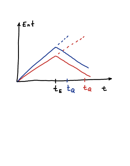
Figure 3: A schematic description of Page’s like curve for de Sitter for different numbers of species. The blue curve corresponds to a higher number $N_{\rm sp}$ than the red one. The corresponding quantum break-times $t_{Q}$ are denoted by the same colors as the curves. Unlike a black hole case, the curve cannot be extended beyond the quantum break-time $t_{Q}$. This time formally equals to a would-be Page’s time but in de Sitter has a fundamentally different effect. The growth is terminated by the graceful exit that takes place at $t_{E}\leqslant t_{Q}$.

V String Theory

We now wish to discuss some implementations of the species magnifier limit (III.3) in string theory. We shall mostly follow Dvali:2020etd in which the needed expression for string theoretic quantum break-time has been derived. A complementary derivation of quantum break-time (58) in string theory context, was also given in Blumenhagen:2020doa .

The regime (III.3) shows transparently, how the string theory responds to a deformation towards a de Sitter type state. For producing such a deformation, we shall use the standard uplifting of the energy via the tension of (anti)$D$-branes Dvali:1998pa .

For definiteness, we shall work in type IIB in ten dimensions, with string coupling $g_{s}$ and the string scale $M_{s}$. As in Dvali:2020etd , we shall consider the background with number of coincident $D_{9}-\bar{D}_{9}$-brane pairs. The world-volume (open string) physics of this system is rather well-understood (see, Srednicki:1998mq and subsequent papers). Our task is to highlight how the system responds to “de Sitterization”. One response is a finite quantum break-time, which was already derived in Dvali:2020etd . Here, we wish to show that this time-scale carries a string theoretic information about the Gibbons-Hawking entropy.

In string construction, the role of $M_{*}$ is played by $M_{s}$. The roles of the low energy species are played by the zero modes of the open strings. With $n$ $D_{9}$-branes and $n$ anti-$D_{9}$-branes piled-up on top of each other, there exist $N_{\rm sp}\sim n^{2}$ light Chan-Paton species. They come from the zero modes of the open strings and transform under the $U(n)\times U(n)$ gauge symmetry.

Of course, such a configuration is unstable since $D$-branes and anti-$D$-branes can annihilate each other. This instability is manifested by an open string tachyon. The $D-\bar{D}$ annihilation can be described as tachyon condensation Sen:1999mg . During this condensation the gauge symmetry is partially Higgsed and the Chan-Paton species become massive. In the original “brane inflation” scenario Dvali:1998pa , the tachyon condensation was used as the graceful exit mechanism from the inflationary phase.

In the present discussion, the main interest is the un-condenced phase, in which tachyon is placed on top of the “hill”. Classically, such a phase can produce a de Sitter like metric with the curvature radius,

$$R=\frac{1}{\sqrt{ng_{s}}M_{s}}\,.$$ (67)

Viewing this as a coherent state of gravitons, we can estimate the number $N$ of the constituent master modes. Since each constituent brings roughly the energy $1/R$, we can determine $N$ by matching $N/R$ with the energy of the Hubble patch. This gives,

$$N=\frac{1}{g_{s}^{2}(ng_{s})^{4}}\,.$$ (68)

It is easy to see that this quantity equals to a Gibbons-Hawking entropy of a would-be ten dimensional de Sitter with the radius (67):

$$S_{GH}=(RM_{10})^{8}=\frac{1}{g_{s}^{2}(ng_{s})^{4}}\,,$$ (69)

where $M_{10}$ denotes the ten-dimensional Planck mass, related to $M_{s}$ and $g_{s}$ through,

$$M_{10}^{8}=\frac{M_{s}^{8}}{g_{s}^{2}}\,.$$ (70)

On the other hand, the ten-dimensional quantum coupling of gravitons of wavelength $R$ (67), is given by,

$$\alpha=\frac{1}{(RM_{10})^{8}}=g_{s}^{2}(ng_{s})^{4}\,.$$ (71)

The equations (68), (69) and (71) confirm that a (would-be) de Sitter obtained in this construction is a saturated state (40).

At the same time, the species coupling (18) is equal to

$$\lambda=\alpha n^{2}=(ng_{s})^{6}\,.$$ (72)

The corresponding quantum break-time, according to (58), is given by

$$t_{Q}=\frac{1}{M_{s}}\frac{1}{(ng_{s})^{13/2}}=\frac{R}{(ng_{s})^{6}}=\frac{R}{\lambda}\,.$$ (73)

This expression was already derived in Dvali:2020etd .

We shall now take the species magnifier limit (III.3). In the present case, this limit reads:

$$n\rightarrow\infty\,,~{}g_{s}\rightarrow 0\,,~{}\lambda=(ng_{s})^{6}={\rm finite}\,,$$ (74)

$$M_{s}={\rm finite}\,,~{}R={\rm finite}\,.$$

In this limit, all stringy processes that are not accompanied by proper powers of $N$ or $n$, vanish. Notice, the quantum break-time (73) remains finite.

For $ng_{s}\ll 1$, the quantum break-time (73) is much longer than the $D$-brane instability time due to tachyon, which is of order $1/M_{s}$. Thus, unless additional stabilizing measures are taken, the tachyon condenses prior to quantum breaking. That is, the tachyon condensation provides a graceful exit that saves the would-be de Sitter from quantum breaking.

What shall happen if we try to stabilize the tachyon? This can be attempted in the following way. Notice that the tachyon coupling to the Chan-Paton species generates an additional contribution to the mass-square of the tachyon field. This is due to their production via Gibbons-Hawking mechanism. The effect can be approximated as coming from a thermal bath of temperature $T_{GH}=1/R$. This generates an effective thermal mass for the tachyon,

$$\Delta m^{2}_{tachyon}=\frac{(ng)^{2}}{R^{2}}=(ng_{s})^{3}M_{s}^{2}\,.$$ (75)

This contribution is positive and could potentially balance the zero-temperature negative mass-square of the tachyon, provided

$$(ng_{s})\sim 1\,.$$ (76)

In this case, the stack of branes could be stabilized.

This stabilization can be viewed as a restoration of $U(n)\times U(n)$ symmetry at high temperature. Such a stabilization of $D$-branes of top of each other by thermal effects has been considered previously (see second reference in Dvali:1998pa ). The difference in the present case is that the stabilization would be “self-imposed” in the sense that it would come from the Gibbons-Hawking temperature created by the brane configuration. That is, branes create de Sitter, which creates a thermal density of open string modes. These thermal corrections, in turn, stabilize the tachyon. This sounds too good to be true. And indeed, there is a caveat.

Notice Dvali:2010vm , (76) represents the point for which the number of Chan-Paton species saturates the ten-dimensional version of the species bound (8),

$$M_{*}=\frac{M_{10}}{N_{\rm sp}^{1/8}}\,.$$ (77)

Taking into account that $M_{*}=M_{s}$ and using the relation (70), we translate (77) as the limiting relation (76) between $n$ and $g_{s}$.

Thinking of the relation (76) as the limit, we notice a rather interesting tendency. This is about entropy of a would-be de Sitter state. Due to the existence of the light Chan-Paton species, we have a non-gravitational contribution to the micro-state entropy. This contribution, roughly, scales as their number ,

$$S_{CP}=n^{2}\,.$$ (78)

We observe that, in the limit (76), the entropy of the open string Chan-Paton species (78), matches the Gibbons-Hawking entropy (69) of a would-be de Sitter state:

$$S_{CP}=S_{GH}=\frac{1}{g_{s}^{2}}\,.$$ (79)

However, at this point, the two critical effects take place in UV and IR theories.

First, the curvature becomes of order the string scale. This is the warning sign from the UV theory. We expect that, beyond this threshold, any notion of the de Sitter geometry is lost. This expectation is fully supported by the knowledge Bowick:1992qu that the Hagedorn effects Hagedorn:1965st set in above the string temperatures. The fundamental stringy effects, such as Atick-Witten phase transition Atick:1988si , must be taken into account. The discussions of aspects of thermal phase can be found in Alvarez:1986sj , Dienes:2012dc , Blumenhagen:2020doa (and references therein). Whatever the theory is in this phase, it is not de Sitter.

It is remarkable, how the low energy theory accounts for this breakdown. First, this is signalled by the fact that the quantum break-time (73) becomes of order the Hubble radius, which is also given by the string length, $t_{Q}\sim 1/M_{s}$.

The second indication from the low energy theory is the behaviour of the scattering amplitudes. Namely, exactly at this point, the processes of graviton-graviton scattering into Chan-Paton species, saturate unitarity bound (40). The example is given by a process in which two gravitons scatter into many Chan-Paton quanta with total occupation number $N=1/\alpha$.

This process falls in the category of generic $2\rightarrow N$ processes of the type (22). As already discussed in section III.1, they saturate unitarity when the entropy of species reaches a critical value (40) Dvali:2020wqi . Near the saturation point the cross-section is given by (25). In the present case, $\alpha$ is given by (71), whereas the entropy $S$ is given by (78). Therefore, around saturation, the cross section can be written as,

$$\sigma={\rm e}^{-n^{2}\left(\frac{1}{(ng_{s})^{6}}-\frac{S_{CP}}{n^{2}}\right)}={\rm e}^{-n^{2}\left(\frac{1}{\lambda}-\frac{S_{CP}}{n^{2}}\right)}\,.$$ (80)

Taking into account (78), the unitarity is saturated for $\lambda\sim 1$. Or equivalently, at the saturation of unitarity by the cross section (80), the open string Chan-Paton entropy matches the Gibbons-Hawking one (79).

Through the above phenomenon, the theory is telling us something profound. In the light of open-closed correspondence, which is intrinsic to string theory, we would expect that the open string sector would carry information about the Gibbons-Hawking entropy of de Sitter vacuum, if such were to exist. And, indeed, we see that the theory does contain such a resource, through the entropy of the open string modes (78). However, this entropy matches the would be Gibbons-Hawking entropy, exactly at the point where unitarity is saturated. Simultaneously, the curvature (67) becomes stringy and so does the quantum break-time (73). As a result, the chance of getting a stable de Sitter state is abolished. This fully matches the conclusion from the previous arguments Dvali:2020etd that de Sitter vacuum is incompatible with non-trivial closed string $S$-matrix.

Notice, none of the above obstructions appear when accounting for Bekenstein-Hawking entropy of an extremal supersymmetric black hole by string degrees of freedom, as it is known from Strominger-Vafa construction Strominger:1996sh . This difference, is also connected with the fact that de Sitter cannot preserve any supersymmetry and, unlike an extremal black hole, exhibits a finite quantum break-time.

Similarly, no quantum breaking is evident to take place (at least in supersymmetric limit) by an anti de Sitter, physics of which is accounted by CFT Maldacena:1997re ; Gubser:1998bc ; Witten:1998qj . We shall leave open the question of possible connection between this physics and the ideas of saturation and corpuscular structure. Some preliminary thoughts can be found in Dvali:2011aa ; Dvali:2013eja .

VI Some Observational Implications

In standard slow-roll picture, the inflaton plays a double role. First, it provides a classical clock that enables inflation to end. Secondly, the quantum fluctuations of this clock provide density perturbations. The quantum corpuscular effects, enhanced by species, interfere with both mechanisms of the inflaton clock.

VI.1 Enhancement of Gibbons-Hawking Perturbations

First, the density fluctuations from Gibbons-Hawking production of species, is enhanced by their number,

$$\delta_{\rm sp}^{2}=\frac{H^{2}}{M_{P}^{2}}N_{\rm sp}\,.$$ (81)

No such enhancement is exhibited by inflaton fluctuations,

$$\delta_{\rm inf}^{2}=\frac{H^{2}}{\epsilon M_{P}^{2}}\,,$$ (82)

where $\epsilon\equiv(V^{\prime}M_{P}/V)^{2}$ is the standard inflationary slow-roll parameter.

Using (8), it is instructive to rewrite the above expressions as functions of $M_{*}$,

$$\delta_{\rm sp}^{2}=\frac{H^{2}}{M_{*}^{2}}\,,~{}\delta_{\rm inf}^{2}=\frac{1}{\epsilon N_{\rm sp}}\frac{H^{2}}{M_{*}^{2}}\,.$$ (83)

We see that in the limit (III.3), which implies $\frac{1}{\epsilon N_{\rm sp}}\rightarrow\infty$, the iflaton perturbations vanish.

We wish to comment that, in case of a large number of light spin-2 species, the enhancement could potentially be experienced by the tensor mode Starobinsky:1979ty .

VI.2 Quantum Clock

As we have seen, the species speed up a different clock in de Sitter. This is an internal quantum clock originating from the corpuscular effects such as depletion, self-entanglement and memory burden. This quantum clock advances regardless of the classical one of a slowly-rolling inflaton field. If the number $N_{\rm sp}$ is above a certain critical value, the quantum clock elapses faster than the classical one. This puts an upper bound on $N_{\rm sp}$.

In general, if the number of species is large, the effect of the quantum clock cannot be ignored. In particular, the tilt in the spectral index will include contributions from two different sources: The standard classical tilt, due to change of $H$, and the quantum one which we shall now quantify.

The quantum clock gives a departure from a (would-be) scale-invariant spectrum of perturbations. This departure is unrelated to a classical slow-roll clock and is due to depletion of the de Sitter constituents. The corresponding tilt in the spectral index can be estimated as,

$$(n_{s}-1)_{\rm Q}=-\frac{N_{sp}H^{2}}{M_{P}^{2}}\,.$$ (84)

This expression for $N_{\rm sp}=1$ was derived in Dvali:2013eja . The effect is enhanced by the number of species Dvali:2020etd .

We shall try to illuminate this phenomenon from various angles. For this, we represent (84) in three equivalent ways,

$$(n_{s}-1)_{\rm Q} = -1/(t_{Q}H)$$

$$= -\frac{H^{2}}{M_{*}^{2}}$$

$$= \lambda\,.$$

An each form, highlights a different physical meaning of the same phenomenon. We shall review them separately.

The first equality in (VI.2) shows that the tilt is the ratio of Hubble-time $1/H$ to quantum break-time $t_{Q}$. This makes sense, since, according to (56), after time $t_{Q}$ the particle-creation rate drops by order one. The effect of the number of species on the tilt is via shortening $t_{Q}$, as it is clear from (58).

The second equality in (VI.2), tells us that the tilt is the square of the ratio of Hubble $H$ to gravity cutoff $M_{*}$. According to (8), the job of the species is to lower $M_{*}$. Correspondingly, they increase the tilt.

Finally, the last equality in (VI.2) tells us that the tilt is equal to the species coupling $\lambda$. Again, the role of the species in increasing tilt is transparent through their contribution into $\lambda$, as described by (18).

Note, the information pattern carried by de Sitter is expected to contribute into the tilt through the memory burden effect, Dvali:2018xpy ; Dvali:2018ytn ; Dvali:2020wft ; Prihadi:2020pqi . Some alternative descriptions can be found in Gomez:2021yhd .

VI.3 Phenomenological Bounds

The large numbers of particle species are included in many extension of the Standard Model. The extreme case is provided by the scenario Dvali:2007hz which incorporates

$$N_{\rm sp}\sim 10^{32}\,.$$ (86)

This number is motivated by the Hierarchy Problem, an outstanding puzzles of the Standard Model. The essence of it is that the mass term of the Higgs scalar is quadratically sensitive to the UV-cutoff of the theory. Ordinarily, the role of the cutoff would be played by $M_{P}$. Hence, having the Higgs mass around $M_{P}$, would raise no concern. However, the Higgs is much lighter than $M_{P}$. This is the source of the puzzle.

The idea of Dvali:2007hz is to use the fact that species lower the cutoff (8). In a theory with $N_{\rm sp}$ given by (86), the cutoff $M_{*}$ is pushed down to its current experimental bound of few TeV. In this case, the Hierarchy Problem gets effectively nullified.

Ordinarily, the inflationary cosmology is assumed to be associated with very high energy scales. In this light, a theory with low cutoff raises concerns because the Hubble parameter has to be small. The perception is that such a theory has a difficulty of generating density perturbations. Again, this concern is coming from an implicit assumption that density perturbations originate from the fluctuations of a single slow-rolling scalar field. However, the same physics that pushed the Hubble down, also provides an alternative mechanism of enhancing the quantum gravitational particle-creation by the number of species. This needs to be taken into account in inflationary model building.

Since (86) represents an absolute phenomenological upper bound on the number of particle species, it is useful to give some examples of enhancement due to this number. For instance, for (86), the observable quantum gravitational imprints can be generated by inflation with the Hubble parameter in a range of nuclear energies, or so.

As another example, a primordial black hole of $10^{-3}$ earth mass, would currently approach its quantum break-time and be at the peak of its Page’s curve. Despite being macroscopic, such a black hole would represent a fully quantum object, with a maximal inner entanglement. Also a memory burden effect would be maximal. A scattering of radiation at such a black hole, would in principle trigger an induced radiation coming from the memory modes. Similar considerations apply to lighter black holes.

The observational prospects, of course, depend on the number density of such black holes. As the preliminary studies indicate Dvali:2020wft , the memory burden effect slows their decay after $t_{Q}$. As suggested, this effect can potentially enlarge the allowed mass window of primordial black holes as dark matter Hawking:1971ei ; Carr:1974nx ; Carr:2016drx towards the lighter end.

VII Outlook: Background Matters

In the present paper we have discussed quantum gravity in species limit (5). This allows to cleanly isolate certain collective and non-perturbative effects that otherwise would be shadowed by irrelevant corrections. The example is a quantum break-time (7), exhibited by saturated systems such as de Sitter and black holes Dvali:2013eja ; Dvali:2014gua ; Dvali:2017eba ; Dvali:2020etd . The species limit (5) allows to keep $t_{Q}$ finite, despite the fact that the perturbative gravity decouples.

Working in the species limit, allows to visualize the time-scales that control the inner entanglement and the back-reaction from the information pattern (memory burden). These are the corpuscular mechanisms that lead the system to quantum breaking.

We extracted the quantum break-time in string theoretic example in which the species are counted by the Chan-Paton factors. This example shows how profoundly the string theory resists to formation of a would-be de Sitter vacuum. The synchronized warning signs are given by low and high energy theories.

The quantum break-time, computed in low energy theory of zero-modes, becomes of order the string length when the high energy theory enters the Hagedorn phase. At the same time, the entropy of the open string modes matches the Gibbons-Hawking entropy. However, this matching takes place at the saturation point of the ten-dimensional species bound (77). This is accompanied by the saturation of the unitarity bound (2) by the entropy of the low energy species.

The above observations, reinforce the earlier conclusions Dvali:2013eja ; Dvali:2014gua ; Dvali:2017eba ; Dvali:2020etd that the finite quantum break-time is the manifestation of inconsistency of the de Sitter state. The same message is carried by more recent conjectures Palti:2019pca .

Next, we wish to put the concept of the exclusion of de Sitter by the $S$-matrix, in a broader perspective of background dependence of quantum gravity. The first point is to take into account the double-scaling argument Dvali:2020etd , which shows that “vacuumization” of de Sitter is linked with trivializing the graviton (closed string) $S$-matrix. Ordinarily, we assume that an approximate $S$-matrix treatment should be valid at short distances. This is true, as long as the short-distance limit commutes with the formulation of the theory.

That is, it is OK to perform an approximate computation, after the theory has been formulated properly. However, there is no a priory justification for doing the same, within a theory that is approximately formulated. The last concept not always makes sense. A good example of such an inconsistency, would be a gauge theory that is approximately anomalous. In fact, the connection between quantum break-time of de Sitter and anomaly was already made in Dvali:2020etd , by drawing a parallel with anomalous $1/N$-effects of Witten-Veneziano mechanism Witten:1979vv .

The second lesson is that, not every background of classical General Relativity, must find its vacuum realization within quantum gravity/string theory. Quantum gravity is more fundamental and more restrictive. It is therefore natural that only certain backgrounds of the classical theory can be given a tittle of a consistent vacuum. Many backgrounds, such as de Sitter, that cannot fit in the vacuum category, must be viewed as excited states constructed on top of a valid $S$-matrix vacuum. They will be subject to severe constraints such as the quantum break-time Dvali:2013eja .

The non-acceptance of all possible classical backgrounds as vacua, must be taken as an advantage of the theory. Needless to say, by eliminating de Sitter vacua, the quantum gravity/string theory nullifies an outstanding cosmological puzzle.

This suggests that the requirement of a background-independent formulation of quantum gravity may not necessarily be the only viable strategy. Rather, an impossibility of formulation of a theory on a given background, can be viewed as a selection tool that increases the restrictive power of the theory.

Acknowledgements

We thank Goran Senjanović for valuable discussions and comments. We thank Alexey Starobinsky for conversation on possible enhancement of the tensor mode. This work was supported in part by the Humboldt Foundation under Humboldt Professorship Award, by the Deutsche Forschungsgemeinschaft (DFG, German Research Foundation) under Germany’s Excellence Strategy - EXC-2111 - 390814868, and Germany’s Excellence Strategy under Excellence Cluster Origins.

References

- (1) G. Dvali and C. Gomez, “Black Hole’s Quantum N-Portrait,” Fortsch. Phys. 61, 742-767 (2013) doi:10.1002/prop.201300001 [arXiv:1112.3359 [hep-th]].
- (2) G. Dvali and C. Gomez, “Black Holes as Critical Point of Quantum Phase Transition,” Eur. Phys. J. C 74, 2752 (2014) doi:10.1140/epjc/s10052-014-2752-3 [arXiv:1207.4059 [hep-th]].
- (3) G. Dvali and C. Gomez, “Quantum Compositeness of Gravity: Black Holes, AdS and Inflation,” JCAP 01, 023 (2014) doi:10.1088/1475-7516/2014/01/023 [arXiv:1312.4795 [hep-th]].
- (4) G. Dvali and C. Gomez, “Quantum Exclusion of Positive Cosmological Constant?,” Annalen Phys. 528, 68-73 (2016) doi:10.1002/andp.201500216 [arXiv:1412.8077 [hep-th]].
- (5) G. Dvali, C. Gomez and S. Zell, “Quantum Break-Time of de Sitter,” JCAP 06, 028 (2017) doi:10.1088/1475-7516/2017/06/028 [arXiv:1701.08776 [hep-th]].
- (6) G. Dvali, “Entropy Bound and Unitarity of Scattering Amplitudes,” J. High Energ. Phys. 2021, 126 (2021). https://doi.org/10.1007/JHEP03(2021)126 [arXiv:2003.05546 [hep-th]].
- (7) G. Dvali, “Area Law Saturation of Entropy Bound from Perturbative Unitarity in Renormalizable Theories,” Fortsch. Phys. 69, no.1, 2000090 (2021) doi:10.1002/prop.202000090 [arXiv:1906.03530 [hep-th]]; “Unitarity Entropy Bound: Solitons and Instantons,” Fortsch. Phys. 69, no.1, 2000091 (2021) doi:10.1002/prop.202000091 [arXiv:1907.07332 [hep-th]].
- (8) J. D. Bekenstein, “Black holes and entropy,” Phys. Rev. D 7, 2333-2346 (1973) doi:10.1103/PhysRevD.7.2333
- (9) G. W. Gibbons and S. W. Hawking, “Cosmological Event Horizons, Thermodynamics, and Particle Creation,” Phys. Rev. D 15, 2738-2751 (1977) doi:10.1103/PhysRevD.15.2738
- (10) G. Dvali, “Black Holes and Large N Species Solution to the Hierarchy Problem,” Fortsch. Phys. 58, 528-536 (2010) doi:10.1002/prop.201000009 [arXiv:0706.2050 [hep-th]]. G. Dvali and M. Redi, “Black Hole Bound on the Number of Species and Quantum Gravity at LHC,” Phys. Rev. D 77, 045027 (2008) doi:10.1103/PhysRevD.77.045027 [arXiv:0710.4344 [hep-th]]. G. Dvali, “Nature of Microscopic Black Holes and Gravity in Theories with Particle Species,” Int. J. Mod. Phys. A 25, 602-615 (2010) doi:10.1142/S0217751X10048895 [arXiv:0806.3801 [hep-th]].
- (11) G. Dvali, “-Matrix and Anomaly of de Sitter,” Symmetry 13, no.1, 3 (2020) doi:10.3390/sym13010003 [arXiv:2012.02133 [hep-th]].
- (12) G. Dvali, D. Flassig, C. Gomez, A. Pritzel and N. Wintergerst, “Scrambling in the Black Hole Portrait,” Phys. Rev. D 88, no.12, 124041 (2013) doi:10.1103/PhysRevD.88.124041 [arXiv:1307.3458 [hep-th]].
- (13) G. Dvali, “A Microscopic Model of Holography: Survival by the Burden of Memory,” [arXiv:1810.02336 [hep-th]].
- (14) G. Dvali, L. Eisemann, M. Michel and S. Zell, “Universe’s Primordial Quantum Memories,” JCAP 03, 010 (2019) doi:10.1088/1475-7516/2019/03/010 [arXiv:1812.08749 [hep-th]].
- (15) G. Dvali, L. Eisemann, M. Michel and S. Zell, “Black hole metamorphosis and stabilization by memory burden,” Phys. Rev. D 102, no.10, 103523 (2020) doi:10.1103/PhysRevD.102.103523 [arXiv:2006.00011 [hep-th]].
- (16) E. Witten, “Quantum gravity in de Sitter space,” [arXiv:hep-th/0106109 [hep-th]].
- (17) D. N. Page, “Information in black hole radiation,” Phys. Rev. Lett. 71, 3743-3746 (1993) doi:10.1103/PhysRevLett.71.3743 [arXiv:hep-th/9306083 [hep-th]].
- (18) S. W. Hawking, “Particle Creation by Black Holes,” Commun. Math. Phys. 43, 199-220 (1975) [erratum: Commun. Math. Phys. 46, 206 (1976)] doi:10.1007/BF02345020.
- (19) G. Dvali and C. Gomez, “Quantum Information and Gravity Cutoff in Theories with Species,” Phys. Lett. B 674, 303-307 (2009) doi:10.1016/j.physletb.2009.03.024 [arXiv:0812.1940 [hep-th]].
- (20) G. Dvali and S. N. Solodukhin, “Black Hole Entropy and Gravity Cutoff,” [arXiv:0806.3976 [hep-th]].
- (21) R. Brustein, G. Dvali and G. Veneziano, “A Bound on the effective gravitational coupling from semiclassical black holes,” JHEP 10, 085 (2009) doi:10.1088/1126-6708/2009/10/085 [arXiv:0907.5516 [hep-th]].
- (22) E. Palti, “The Swampland: Introduction and Review,” Fortsch. Phys. 67, no.6, 1900037 (2019) doi:10.1002/prop.201900037 [arXiv:1903.06239 [hep-th]].
- (23) G. Dvali and D. Lust, “Power of Black Hole Physics: Seeing through the Vacuum Landscape,” JHEP 06, 047 (2008) doi:10.1088/1126-6708/2008/06/047 [arXiv:0801.1287 [hep-th]].
- (24) G. R. Dvali, G. Gabadadze, M. Kolanović and F. Nitti, “Scales of gravity,” Phys. Rev. D 65, 024031 (2002) doi:10.1103/PhysRevD.65.024031 [arXiv:hep-th/0106058 [hep-th]].
- (25) G. Veneziano, “Large N bounds on, and compositeness limit of, gauge and gravitational interactions,” JHEP 06, 051 (2002) doi:10.1088/1126-6708/2002/06/051 [arXiv:hep-th/0110129 [hep-th]];
- (26) G. ’t Hooft, “A Planar Diagram Theory for Strong Interactions,” Nucl. Phys. B 72, 461 (1974) doi:10.1016/0550-3213(74)90154-0
- (27) A. A. Starobinsky, “Spectrum of relict gravitational radiation and the early state of the universe,” JETP Lett. 30, 682-685 (1979)
- (28) G. Dvali, C. Gomez, R. S. Isermann, D. Lüst and S. Stieberger, “Black hole formation and classicalization in ultra-Planckian scattering,” Nucl. Phys. B 893, 187-235 (2015) doi:10.1016/j.nuclphysb.2015.02.004 [arXiv:1409.7405 [hep-th]].
- (29) A. Addazi, M. Bianchi and G. Veneziano, “Glimpses of black hole formation/evaporation in highly inelastic, ultra-planckian string collisions,” JHEP 02, 111 (2017) doi:10.1007/JHEP02(2017)111 [arXiv:1611.03643 [hep-th]].
- (30) F. Kühnel, “Thoughts on the Vacuum Energy in the Quantum N-Portrait,” Mod. Phys. Lett. A 30, no.36, 1550197 (2015) doi:10.1142/S0217732315501977 [arXiv:1408.5897 [gr-qc]].
- (31) F. Kuhnel and M. Sandstad, “Corpuscular Consideration of Eternal Inflation,” Eur. Phys. J. C 75, no.10, 505 (2015) doi:10.1140/epjc/s10052-015-3736-7 [arXiv:1504.02377 [gr-qc]].
- (32) R. Casadio, F. Kuhnel and A. Orlandi, “Consistent Cosmic Microwave Background Spectra from Quantum Depletion,” JCAP 09, 002 (2015) doi:10.1088/1475-7516/2015/09/002 [arXiv:1502.04703 [gr-qc]].
- (33) L. Berezhiani, “On Corpuscular Theory of Inflation,” Eur. Phys. J. C 77, no.2, 106 (2017) doi:10.1140/epjc/s10052-017-4672-5 [arXiv:1610.08433 [hep-th]].
- (34) S. Brahma, K. Dasgupta and R. Tatar, “Four-dimensional de Sitter space is a Glauber-Sudarshan state in string theory,” [arXiv:2007.00786 [hep-th]]; “de Sitter Space as a Glauber-Sudarshan State,” JHEP 02, 104 (2021) doi:10.1007/JHEP02(2021)104 [arXiv:2007.11611 [hep-th]].
- (35) G. ’t Hooft, “Graviton Dominance in Ultrahigh-Energy Scattering,” Phys. Lett. B 198, 61-63 (1987) doi:10.1016/0370-2693(87)90159-6
- (36) D. Amati, M. Ciafaloni and G. Veneziano, “Superstring Collisions at Planckian Energies,” Phys. Lett. B 197, 81 (1987) doi:10.1016/0370-2693(87)90346-7
- (37) D. J. Gross and P. F. Mende, “The High-Energy Behavior of String Scattering Amplitudes,” Phys. Lett. B 197, 129-134 (1987) doi:10.1016/0370-2693(87)90355-8
- (38) G. Dvali, “Area law microstate entropy from criticality and spherical symmetry,” Phys. Rev. D 97, no.10, 105005 (2018) doi:10.1103/PhysRevD.97.105005 [arXiv:1712.02233 [hep-th]].
- (39) G. Dvali, M. Michel and S. Zell, “Finding Critical States of Enhanced Memory Capacity in Attractive Cold Bosons,” EPJ Quant. Technol. 6, 1 (2019) doi:10.1140/epjqt/s40507-019-0071-1 [arXiv:1805.10292 [quant-ph]].
- (40) G. Dvali and S. Zell, “Classicality and Quantum Break-Time for Cosmic Axions,” JCAP 07, 064 (2018) doi:10.1088/1475-7516/2018/07/064 [arXiv:1710.00835 [hep-ph]].
- (41) A. Kovtun and M. Zantedeschi, “Breaking BEC,” JHEP 07, 212 (2020) doi:10.1007/JHEP07(2020)212 [arXiv:2003.10283 [hep-th]].
- (42) A. Kovtun and M. Zantedeschi, “Breaking BEC: the fast and the quantum,” [arXiv:2008.02187 [hep-th]].
- (43) L. Berezhiani and M. Zantedeschi, “On Evolution of Coherent States as Quantum Counterpart of Classical Dynamics,” [arXiv:2011.11229 [hep-th]].
- (44) R. Blumenhagen, C. Kneissl and A. Makridou, “De Sitter Quantum Breaking, Swampland Conjectures and Thermal Strings,” [arXiv:2011.13956 [hep-th]].
- (45) H. L. Prihadi, D. Dwiputra and F. P. Zen, “Long-range correlation of CMB temperature fluctuations from the holographic entanglement entropy,” [arXiv:2005.00981 [hep-th]].
- (46) G. Dvali, C. Gomez and D. Lust, “Black Hole Quantum Mechanics in the Presence of Species,” Fortsch. Phys. 61, 768-778 (2013) doi:10.1002/prop.201300002 [arXiv:1206.2365 [hep-th]].
- (47) R. Hagedorn, “Statistical thermodynamics of strong interactions at high-energies,” Nuovo Cim. Suppl. 3, 147-186 (1965) CERN-TH-520.
- (48) M. J. Bowick, “Finite temperature strings,” [arXiv:hep-th/9210016 [hep-th]].
- (49) G. R. Dvali and S. H. H. Tye, “Brane inflation,” Phys. Lett. B 450, 72-82 (1999) doi:10.1016/S0370-2693(99)00132-X [arXiv:hep-ph/9812483 [hep-ph]]. For various implementations of this mechanism, see, G. R. Dvali, “Infrared hierarchy, thermal brane inflation and superstrings as superheavy dark matter,” Phys. Lett. B 459, 489-496 (1999) doi:10.1016/S0370-2693(99)00726-1 [arXiv:hep-ph/9905204 [hep-ph]]. G. R. Dvali, Q. Shafi and S. Solganik, “D-brane inflation,” [arXiv:hep-th/0105203 [hep-th]]. C. P. Burgess, M. Majumdar, D. Nolte, F. Quevedo, G. Rajesh and R. J. Zhang, “The Inflationary brane anti-brane universe,” JHEP 07, 047 (2001) doi:10.1088/1126-6708/2001/07/047 [arXiv:hep-th/0105204 [hep-th]]. S. Kachru, R. Kallosh, A. D. Linde and S. P. Trivedi, “De Sitter vacua in string theory,” Phys. Rev. D 68, 046005 (2003) doi:10.1103/PhysRevD.68.046005 [arXiv:hep-th/0301240 [hep-th]]. S. Kachru, R. Kallosh, A. D. Linde, J. M. Maldacena, L. P. McAllister and S. P. Trivedi, “Towards inflation in string theory,” JCAP 10, 013 (2003) doi:10.1088/1475-7516/2003/10/013 [arXiv:hep-th/0308055 [hep-th]].
- (50) M. Srednicki, “IIB or not IIB,” JHEP 08, 005 (1998) doi:10.1088/1126-6708/1998/08/005 [arXiv:hep-th/9807138 [hep-th]].
- (51) G. Dvali and C. Gomez, “Species and Strings,” [arXiv:1004.3744 [hep-th]].
- (52) See, e.g., A. Sen, “NonBPS states and Branes in string theory,” [arXiv:hep-th/9904207 [hep-th]].
- (53) J. J. Atick and E. Witten, “The Hagedorn Transition and the Number of Degrees of Freedom of String Theory,” Nucl. Phys. B 310, 291-334 (1988) doi:10.1016/0550-3213(88)90151-4
- (54) E. Alvarez and M. A. R. Osorio, “Superstrings at Finite Temperature,” Phys. Rev. D 36, 1175 (1987) doi:10.1103/PhysRevD.36.1175
- (55) K. R. Dienes, M. Lennek and M. Sharma, “Strings at Finite Temperature: Wilson Lines, Free Energies, and the Thermal Landscape,” Phys. Rev. D 86, 066007 (2012) doi:10.1103/PhysRevD.86.066007 [arXiv:1205.5752 [hep-th]].
- (56) A. Strominger and C. Vafa, “Microscopic origin of the Bekenstein-Hawking entropy,” Phys. Lett. B 379, 99-104 (1996) doi:10.1016/0370-2693(96)00345-0 [arXiv:hep-th/9601029 [hep-th]].
- (57) J. M. Maldacena, “The Large N limit of superconformal field theories and supergravity,” Adv. Theor. Math. Phys. 2, 231-252 (1998) doi:10.1023/A:1026654312961 [arXiv:hep-th/9711200 [hep-th]].
- (58) S. S. Gubser, I. R. Klebanov and A. M. Polyakov, “Gauge theory correlators from noncritical string theory,” Phys. Lett. B 428, 105-114 (1998) doi:10.1016/S0370-2693(98)00377-3 [arXiv:hep-th/9802109 [hep-th]].
- (59) E. Witten, “Anti-de Sitter space and holography,” Adv. Theor. Math. Phys. 2, 253-291 (1998) doi:10.4310/ATMP.1998.v2.n2.a2 [arXiv:hep-th/9802150 [hep-th]].
- (60) C. Gómez and R. Jimenez, “Model Independent Prediction of the Spectral Index of Primordial Quantum Fluctuations,” [arXiv:2103.10144 [hep-th]].
- (61) S. Hawking, “Gravitationally collapsed objects of very low mass,” Mon. Not. Roy. Astron. Soc. 152, 75 (1971)
- (62) B. J. Carr and S. W. Hawking, “Black holes in the early Universe,” Mon. Not. Roy. Astron. Soc. 168, 399-415 (1974)
- (63) B. Carr, F. Kuhnel and M. Sandstad, “Primordial Black Holes as Dark Matter,” Phys. Rev. D 94, no.8, 083504 (2016) doi:10.1103/PhysRevD.94.083504 [arXiv:1607.06077 [astro-ph.CO]].
- (64) E. Pajer, D. Stefanyszyn and J. Supeł, “The Boostless Bootstrap: Amplitudes without Lorentz boosts,” JHEP 12, 198 (2020) doi:10.1007/JHEP12(2020)198 [arXiv:2007.00027 [hep-th]].
- (65) V. Gorbenko and L. Senatore, “ in dS,” [arXiv:1911.00022 [hep-th]].
- (66) E. Witten, “Current Algebra Theorems for the U(1) Goldstone Boson,” Nucl. Phys. B 156, 269-283 (1979) doi:10.1016/0550-3213(79)90031-2; G. Veneziano, “U(1) Without Instantons,” Nucl. Phys. B 159, 213-224 (1979) doi:10.1016/0550-3213(79)90332-8