Laser-induced torques in metallic antiferromagnets

Abstract

We study the laser-induced torques in the antiferromagnet (AFM) Mn₂Au. We find that even linearly polarized light may induce laser-induced torques in Mn₂Au, i.e., the light does not have to be circularly polarized. The laser-induced torques in Mn₂Au are comparable in magnitude to those in the ferromagnets Fe, Co and FePt at optical frequencies. We also compute the laser-induced torques at terahertz (THz) frequencies and compare them to the spin-orbit torques (SOTs) excited by THz laser-pulses. We find the SOTs to be dominant at THz frequencies for the laser-field strengths used in experiments. Additionally, we show that the matrix elements of the spin-orbit interaction (SOI) can be used to add SOI only during the Wannier interpolation, which we call Wannier interpolation of SOI (WISOI). This technique allows us to perform the Wannier interpolation conveniently for many magnetization directions from a single set of Wannier functions.

I Introduction

Using femtosecond laser-pulses to switch the magnetization [1, 2], to exert torques on the magnetic moments [3, 4, 5, 6, 7, 8, 9, 10, 11], to move domain walls [12], and to excite magnons [13] are promising concepts to write, store and process information on ultrafast timescales in prospective device applications. In bulk crystals laser-induced torques on the magnetization are attributed to the inverse Faraday effect (IFE) and to the optical spin-transfer torque (OSTT) [3, 4, 11]. Phenomenology for non-magnets predicts the IFE only for circularly polarized light. However, works on the ferromagnetic Rashba model [14] as well as first-principles calculations [11, 15] show that the IFE in ferromagnets differs from these predictions, i.e., the IFE is present even for linearly polarized light.

Due to their terahertz (THz) magnetization dynamics, antiferromagnets (AFMs) are another promising ingredient in ultrafast magnetism concepts [16, 17, 18, 19]. To this end, spin-orbit torques (SOTs) in the bulk AFM Mn₂Au have been studied intensively both in theory [20, 21, 22] and in experiment [23, 24, 25, 26] and it has been shown that the SOT may be used to switch the Néel vector. For the optical manipulation of the Néel vector the IFE and OSTT might be promising alternatives to the SOT. However, theoretical works on the IFE and OSTT in antiferromagnets (AFM) are still lacking.

When lasers at optical frequencies are used to exert torques in AFMs it is clear that the SOT excited by the electric field of the laser may be ignored, because it is oscillating at the laser frequency, which is far above the magnetic resonances in the AFMs in the THz range. This picture changes when THz lasers are used to excite the magnetization in AFMs. In Ref. [19] THz laser pulses were used to switch the AFM CuMnAs contactlessly and this switching was interpreted as the action of the SOT. While the SOT is linear in the applied electric field, the IFE and OSTT are quadratic in it. The question therefore arises at which electric field strength the IFE and OSTT become more important than the SOT when the frequency of the applied electric field is in the THz range.

In this work we investigate the laser-induced torques in the bulk AFM Mn₂Au. Our computational approach is based on the Keldysh nonequilibrium formalism and on the Wannier interpolation [27] of the electronic structure obtained from realistic density-functional theory calculations. In order to study the dependence of the laser-induced torques on the magnetization direction we introduce a method that allows us to do the Wannier interpolation conveniently for many different magnetization directions on the basis of a single set of maximally localized Wannier functions (MLWFs), which we call Wannier interpolation of SOI (WISOI).

This paper is organized as follows. In Sec. II.1 we briefly review the formalism that we use to compute the laser-induced torque. In Sec. II.2 we describe WISOI briefly, deferring details on the implementation to Appendix A. In Sec. II.3 we discuss how the symmetry of the Mn₂Au crystal determines the form of the response tensor. In Sec. III we discuss our results on the laser-induced torques in Mn₂Au. This paper ends with a summary in Sec. IV.

II Formalism

II.1 Keldysh formalism

In Ref. [11] we derived the following expression for the laser-induced torque based on the Keldysh nonequilibrium formalism:

$$T_{i}=\frac{a_{0}^{3}I}{c}\left(\frac{\mathcal{E}_{\rm H}}{\hbar\omega}\right)^{2}{\rm Im}\sum_{jk}\epsilon_{j}\epsilon_{k}^{*}\chi_{ijk},$$ (1)

where $c$ is the velocity of light, $a_{0}=4\pi\epsilon_{0}\hbar^{2}/(me^{2})$ is Bohr’s radius, $I=\epsilon_{0}cE_{0}^{2}/2$ is the intensity of light, $\epsilon_{0}$ is the vacuum permittivity, $\mathcal{E}_{\rm H}=e^{2}/(4\pi\epsilon_{0}a_{0})$ is the Hartree energy, and $\epsilon_{j}$ is the $j$-th Cartesian component of the light polarization vector. The tensor $\chi_{ijk}$ is given by

$$\chi_{ijk}= \frac{2}{\mathcal{N}\hbar a_{0}^{2}\mathcal{E}_{\rm H}}\sum_{{\boldsymbol{k}}}\int{\rm d}\mathcal{E}{\rm Tr}\Big{[}$$ (2)

$$f(\mathcal{E})\mathcal{T}_{i}G^{\rm R}_{{\boldsymbol{k}}}(\mathcal{E})v_{j}G^{\rm R}_{{\boldsymbol{k}}}(\mathcal{E}-\hbar\omega)v_{k}G^{\rm R}_{{\boldsymbol{k}}}(\mathcal{E})$$

$$- f(\mathcal{E})\mathcal{T}_{i}G^{\rm R}_{{\boldsymbol{k}}}(\mathcal{E})v_{j}G^{\rm R}_{{\boldsymbol{k}}}(\mathcal{E}-\hbar\omega)v_{k}G^{\rm A}_{{\boldsymbol{k}}}(\mathcal{E})$$

$$+ f(\mathcal{E})\mathcal{T}_{i}G^{\rm R}_{{\boldsymbol{k}}}(\mathcal{E})v_{k}G^{\rm R}_{{\boldsymbol{k}}}(\mathcal{E}+\hbar\omega)v_{j}G^{\rm R}_{{\boldsymbol{k}}}(\mathcal{E})$$

$$- f(\mathcal{E})\mathcal{T}_{i}G^{\rm R}_{{\boldsymbol{k}}}(\mathcal{E})v_{k}G^{\rm R}_{{\boldsymbol{k}}}(\mathcal{E}+\hbar\omega)v_{j}G^{\rm A}_{{\boldsymbol{k}}}(\mathcal{E})$$

$$+ f(\mathcal{E}-\hbar\omega)\mathcal{T}_{i}G^{\rm R}_{{\boldsymbol{k}}}(\mathcal{E})v_{j}G^{\rm R}_{{\boldsymbol{k}}}(\mathcal{E}-\hbar\omega)v_{k}G^{\rm A}_{{\boldsymbol{k}}}(\mathcal{E})$$

$$+ f(\mathcal{E}+\hbar\omega)\mathcal{T}_{i}G^{\rm R}_{{\boldsymbol{k}}}(\mathcal{E})v_{k}G^{\rm R}_{{\boldsymbol{k}}}(\mathcal{E}+\hbar\omega)v_{j}G^{\rm A}_{{\boldsymbol{k}}}(\mathcal{E})\Big{]},$$

where $\mathcal{N}$ is the number of ${\boldsymbol{k}}$ points, $f(\mathcal{E})$ is the Fermi distribution function, ${\boldsymbol{\mathcal{T}}}$ is the torque operator, ${\boldsymbol{v}}$ is the velocity operator,

$$G^{\rm R}_{{\boldsymbol{k}}}(\mathcal{E})=\hbar\sum_{n}\frac{|{\boldsymbol{k}}n\rangle\langle{\boldsymbol{k}}n|}{\mathcal{E}-\mathcal{E}_{{\boldsymbol{k}}n}+i\Gamma},$$ (3)

is the retarded Green function and $G^{\rm A}_{{\boldsymbol{k}}}(\mathcal{E})=[G^{\rm R}_{{\boldsymbol{k}}}(\mathcal{E})]^{\dagger}$ is the advanced Green function. Here, $|{\boldsymbol{k}}n\rangle$ and $\mathcal{E}_{{\boldsymbol{k}}n}$ are eigenstates and eigenenergies, respectively, and $\Gamma$ is a constant broadening used to simulate disorder and finite lifetimes of the electronic states.

Our Green’s function expressions provide an alternative approach to the expressions based on the order formalism [28, 15] used to compute the IFE. In Ref. [29] we have shown that Eq. (2) may be modified in order to compute laser-induced charge and spin photocurrents. Thus, the Keldysh formalism underlying Eq. (2) provides also an alternative approach to the method based on the expressions given first by von Baltz and Kraut [30, 31, 32].

In the case of the SOT one may distinguish spin and orbital torques [33, 34, 35, 36, 22, 37]. For example in TmIG/Pt/CuO_x the SOT has been interpreted in terms of an orbital current generated at the Pt/CuO_x interface, which is converted subsequently into a spin current by the SOI of Pt [34], and in Ni/W(110) calculations show that the SOT even differs in sign from the spin-transfer torque associated with the spin current of W [33] because the orbital torque dominates. However, when one computes the linear response of the torque operator ${\boldsymbol{\mathcal{T}}}$ to the applied electric field one captures both the spin torque and the orbital torque. Therefore, in order to describe the SOT when the orbital torque is dominating, one does not need a new formalism to compute the total SOT, but one might wish to develop additional tools to separate the total SOT into spin and orbital contributions [33].

In the case of the laser-induced torques it might become useful as well to distinguish between spin and orbital contributions. A strong indication that this might be the case is the finding of a large laser-induced orbital magnetization [15] even without SOI. However, the only mechanism by which this orbital magnetization may directly lead to a torque on the magnetization is through the Oersted field generated by the orbital photocurrent. Therefore, one may expect that a significantly larger torque arises from the coupling of the laser-induced orbital magnetization to the spin magnetization due to SOI. Such an indirect contribution from the laser-induce orbital magnetization to the laser-induced torque is already contained in the response of the torque operator ${\boldsymbol{\mathcal{T}}}$ to the applied laser field and an extension of our formalism is not necessary. However, like in the case of the SOT, it might become desirable in the future to develop tools to separate the laser-induced torque into spin and orbital contributions. We leave the development of such tools for future work.

II.2 Wannier interpolation of SOI (WISOI)

In the presence of SOI the electronic structure depends on the direction of the (staggered) magnetization. When one would like to evaluate Eq. (2) for many different magnetization directions one first needs to perform DFT calculations of the electronic structure for all of them. If one uses Wannier interpolation for computational speed-up of Eq. (2) one additionally needs to compute MLWFs for all these magnetization directions. Alternatively, one may compute the electronic structure and MLWFs without SOI and add the effect of SOI during the Wannier interpolation of the material property tensors. This is a very convenient approach when the material property tensors need to be evaluated for many magnetization directions.

We briefly explain this Wannier interpolation of SOI here and refer the reader to the appendix A for the details of our implementation of this approach. We denote the MLWFs without SOI by $|\bar{W}_{{\boldsymbol{R}}n\sigma}\rangle$, where $\sigma=\uparrow,\downarrow$ labels the spin. The number of spin-up MLWFs is $N_{\uparrow}$ and the number of spin-down MLWFs is $N_{\downarrow}$. The total number of MLWFs is $N_{\rm W}=N_{\uparrow}+N_{\downarrow}$. Using these MLWFs, we compute the matrix elements of the Hamiltonian $\bar{H}$ without SOI

$$\bar{h}^{\sigma\sigma}_{{\boldsymbol{R}}nm} =\langle\bar{W}_{{\boldsymbol{0}}n\sigma}|\bar{H}|\bar{W}_{{\boldsymbol{R}}m\sigma}\rangle$$ (4)

and additionally the following matrix elements:

$$\mathcal{A}^{\sigma\sigma^{\prime}j}_{{\boldsymbol{R}}nm}=\sum_{\alpha}\langle\bar{W}_{{\boldsymbol{0}}n\sigma}|\xi_{\alpha}({\boldsymbol{r}}-{\boldsymbol{r}}_{\alpha})L_{j}^{\alpha}|\bar{W}_{{\boldsymbol{R}}m\sigma^{\prime}}\rangle,$$ (5)

where $L_{j}^{\alpha}$ is the orbital angular momentum operator of atom $\alpha$ and $\xi_{\alpha}({\boldsymbol{r}}-{\boldsymbol{r}}_{\alpha})$ is the SOI potential in a sphere around atom $\alpha$ with its center at ${\boldsymbol{r}}_{\alpha}$. The index $j$ takes the values $z$, $-$, and $+$, where $L^{\alpha}_{+}=(L^{\alpha}_{x}+iL^{\alpha}_{y})$ and $L^{\alpha}_{-}=(L^{\alpha}_{x}-iL^{\alpha}_{y})$.

One needs to add $\mathcal{V}_{\rm SOI}=\sum_{\alpha}\xi_{\alpha}({\boldsymbol{r}}-{\boldsymbol{r}}_{\alpha}){\boldsymbol{L}}^{\alpha}\cdot{\boldsymbol{\sigma}}$ to $\bar{H}$ in order to include SOI into the calculation. To obtain the matrix elements $\mathcal{V}^{\sigma\sigma^{\prime}}_{{\boldsymbol{R}}nm}=\langle\bar{W}_{{\boldsymbol{0}}n\sigma}|\mathcal{V}_{\rm SOI}|\bar{W}_{{\boldsymbol{R}}m\sigma^{\prime}}\rangle$ when the Néel vector points into the direction $\hat{{\boldsymbol{\mathcal{L}}}}=(\sin\theta\cos\phi,\sin\theta\sin\phi,\cos\theta)^{\rm T}$ we need to multiply the Eq. (5) with trigonometric functions of the angles $\theta$ and $\phi$ as follows:

$${\boldsymbol{\mathcal{V}}}^{\uparrow\uparrow}_{{\boldsymbol{R}}} ={\boldsymbol{\mathcal{A}}}^{\uparrow\uparrow z}_{{\boldsymbol{R}}}\cos\theta+\frac{1}{2}{\boldsymbol{\mathcal{A}}}^{\uparrow\uparrow-}_{{\boldsymbol{R}}}\sin\theta{\rm e}^{i\phi}+\frac{1}{2}{\boldsymbol{\mathcal{A}}}^{\uparrow\uparrow+}_{{\boldsymbol{R}}}\sin\theta{\rm e}^{-i\phi},$$ (6)

$${\boldsymbol{\mathcal{V}}}^{\downarrow\downarrow}_{{\boldsymbol{R}}} =-{\boldsymbol{\mathcal{A}}}^{\downarrow\downarrow z}_{{\boldsymbol{R}}}\cos\theta-\frac{1}{2}{\boldsymbol{\mathcal{A}}}^{\downarrow\downarrow-}_{{\boldsymbol{R}}}\sin\theta{\rm e}^{i\phi}-\frac{1}{2}{\boldsymbol{\mathcal{A}}}^{\downarrow\downarrow+}_{{\boldsymbol{R}}}\sin\theta{\rm e}^{-i\phi},$$ (7)

$${\boldsymbol{\mathcal{V}}}^{\uparrow\downarrow}_{{\boldsymbol{R}}} =-{\boldsymbol{\mathcal{A}}}^{\uparrow\downarrow z}_{{\boldsymbol{R}}}\sin\theta+{\boldsymbol{\mathcal{A}}}^{\uparrow\downarrow-}_{{\boldsymbol{R}}}\left[\cos\frac{\theta}{2}\right]^{2}{\rm e}^{i\phi}-{\boldsymbol{\mathcal{A}}}^{\uparrow\downarrow+}_{{\boldsymbol{R}}}\left[\sin\frac{\theta}{2}\right]^{2}{\rm e}^{-i\phi},$$ (8)

and

$${\boldsymbol{\mathcal{V}}}^{\downarrow\uparrow}_{{\boldsymbol{R}}} =-{\boldsymbol{\mathcal{A}}}^{\downarrow\uparrow z}_{{\boldsymbol{R}}}\sin\theta-{\boldsymbol{\mathcal{A}}}^{\downarrow\uparrow-}_{{\boldsymbol{R}}}\left[\sin\frac{\theta}{2}\right]^{2}e^{i\phi}+{\boldsymbol{\mathcal{A}}}^{\downarrow\uparrow+}_{{\boldsymbol{R}}}\left[\cos\frac{\theta}{2}\right]^{2}e^{-i\phi}.$$ (9)

Finally, the Wannier-interpolated Hamiltonian matrix including SOI is given by

$$H_{{\boldsymbol{k}}}^{\rm W}=\begin{pmatrix}\bar{{\boldsymbol{h}}}^{\uparrow\uparrow}_{{\boldsymbol{k}}}&0\\ 0&\bar{{\boldsymbol{h}}}^{\downarrow\downarrow}_{{\boldsymbol{k}}}\end{pmatrix}+\begin{pmatrix}{\boldsymbol{\mathcal{V}}}^{\uparrow\uparrow}_{{\boldsymbol{k}}}&{\boldsymbol{\mathcal{V}}}^{\uparrow\downarrow}_{{\boldsymbol{k}}}\\ {\boldsymbol{\mathcal{V}}}^{\downarrow\uparrow}_{{\boldsymbol{k}}}&{\boldsymbol{\mathcal{V}}}^{\downarrow\downarrow}_{{\boldsymbol{k}}}\end{pmatrix}$$ (10)

where the $N_{\sigma}\times N_{\sigma^{\prime}}$ matrices $\bar{{\boldsymbol{h}}}^{\sigma\sigma^{\prime}}_{{\boldsymbol{k}}}$ and ${\boldsymbol{\mathcal{V}}}^{\sigma\sigma^{\prime}}_{{\boldsymbol{k}}}$ are the following Fourier transforms:

$$\bar{{\boldsymbol{h}}}^{\sigma\sigma^{\prime}}_{{\boldsymbol{k}}}=\sum_{{\boldsymbol{R}}}{\rm e}^{i{\boldsymbol{k}}\cdot{\boldsymbol{R}}}\bar{{\boldsymbol{h}}}^{\sigma\sigma^{\prime}}_{{\boldsymbol{R}}},\quad{\boldsymbol{\mathcal{V}}}^{\sigma\sigma^{\prime}}_{{\boldsymbol{k}}}=\sum_{{\boldsymbol{R}}}{\rm e}^{i{\boldsymbol{k}}\cdot{\boldsymbol{R}}}{\boldsymbol{\mathcal{V}}}^{\sigma\sigma^{\prime}}_{{\boldsymbol{R}}}.$$ (11)

With this Wannier-interpolated Hamiltonian $H_{{\boldsymbol{k}}}^{\rm W}$ we proceed in the usual way, i.e., it is diagonalized and the eigenvalues and eigenvectors are used to evaluate Eq. (2). The velocity operator is obtained from $H_{{\boldsymbol{k}}}^{\rm W}$ as usual [27]:

$${\boldsymbol{v}}_{{\boldsymbol{k}}}=\frac{1}{\hbar}\frac{\partial H_{{\boldsymbol{k}}}^{\rm W}}{\partial{\boldsymbol{k}}}.$$ (12)

II.3 Symmetry

In this section we discuss which components of the tensor $\chi_{ijk}$, Eq. (2), are allowed by symmetry in the Mn₂Au crystal. For this purpose we expand the laser-induced torque in orders of the staggered magnetization $\mathcal{L}$ as follows:

$$T_{i}=\chi^{(\rm{4sp})}_{ijkl}E_{j}E^{*}_{k}\mathcal{L}_{l}+\chi^{(\rm 5a)}_{ijklm}E_{j}E_{k}^{*}\mathcal{L}_{l}\mathcal{L}_{m}+\dots,$$ (13)

which implies that $\chi_{ijk}$ has the expansion

$$\chi_{ijk}=\chi^{(\rm{4sp})}_{ijkl}\mathcal{L}_{l}+\chi^{(\rm 5a)}_{ijklm}\mathcal{L}_{l}\mathcal{L}_{m}+\dots.$$ (14)

First we need to find out how the tensors $\chi^{(\rm{4sp})}_{ijkl}$ and $\chi^{(\rm 5a)}_{ijklm}$ transform under symmetry operations. We recall that polar tensors satisfy

$$\chi^{\rm p}_{i^{\prime}j^{\prime}k^{\prime}l^{\prime}\dots}=\chi^{\rm p}_{ijkl\dots}\mathcal{R}_{ii^{\prime}}\mathcal{R}_{jj^{\prime}}\mathcal{R}_{kk^{\prime}}\mathcal{R}_{ll^{\prime}}\dots$$ (15)

for all symmetry operations $\mathcal{R}$ in the point group of the space group of the crystal, while axial tensors satisfy

$$\chi^{\rm a}_{i^{\prime}j^{\prime}k^{\prime}l^{\prime}\dots}=(-1)^{\rm det\mathcal{R}}\chi^{\rm a}_{ijkl\dots}\mathcal{R}_{ii^{\prime}}\mathcal{R}_{jj^{\prime}}\mathcal{R}_{kk^{\prime}}\mathcal{R}_{ll^{\prime}}\dots.$$ (16)

In general, a staggered field, i.e., a field that switches sign between different magnetic sublattices, transforms differently from a non-staggered field. For this reason the introduction of polar and axial response tensors is insufficient to describe all possible responses in antiferromagnets. Therefore, we need to introduce two more types of tensors, namely staggered polar and staggered axial tensors. In antiferromagnets with two magnetic sublattices that are not related by a lattice translation these two additional types of tensors may be defined as follows: We call a tensor staggered polar when it satisfies

$$\chi^{\rm sp}_{i^{\prime}j^{\prime}k^{\prime}l^{\prime}\dots}=(-1)^{S(\mathcal{R})}\chi^{\rm sp}_{ijkl\dots}\mathcal{R}_{ii^{\prime}}\mathcal{R}_{jj^{\prime}}\mathcal{R}_{kk^{\prime}}\mathcal{R}_{ll^{\prime}}\dots$$ (17)

for all $\mathcal{R}$ in the point group. Here, $S(\mathcal{R})=-1$ if $\mathcal{R}$ interchanges the two sublattices and $S(\mathcal{R})=1$ otherwise. Similarly, we call a tensor staggered axial when it satisfies

$$\chi^{\rm sa}_{i^{\prime}j^{\prime}k^{\prime}l^{\prime}\dots}=(-1)^{S(\mathcal{R})}(-1)^{\rm det\mathcal{R}}\chi^{\rm sa}_{ijkl\dots}\mathcal{R}_{ii^{\prime}}\mathcal{R}_{jj^{\prime}}\mathcal{R}_{kk^{\prime}}\mathcal{R}_{ll^{\prime}}\dots$$ (18)

for all $\mathcal{R}$ in the point group.

The Néel vector $\mathcal{L}$ transforms like a staggered axial tensor of rank 1. Consequently, $\chi^{(\rm{4sp})}_{ijkl}$ is a staggered polar tensor of rank 4 and $\chi^{(\rm 5a)}_{ijklm}$ is an axial tensor of rank 5. Our expansion in Eq. (13) has the advantage that it can be applied for a general direction of ${\boldsymbol{\mathcal{L}}}$ and that only information on the point group and on the positions of the magnetic sublattice sites are required to determine the tensors allowed by symmetry. In contrast, the usual symmetry analysis based on the magnetic point groups suffers from the fact that in the presence of SOI the magnetic point group depends on the direction of ${\boldsymbol{\mathcal{L}}}$. Determining the response tensors allowed by the magnetic point groups for selected high-symmetry directions of ${\boldsymbol{\mathcal{L}}}$ provides less information than our expansion Eq. (13).

Next, we need to find out which components of the tensors are consistent with all symmetry operations $\mathcal{R}$. We find that in Mn₂Au staggered polar tensors of rank 4 are not allowed by symmetry. However, axial tensors of rank 5 are allowed and we find 30 such tensors. In order to discuss these tensors we introduce the notation

$$\delta^{(ijklm)}_{nopqr}=\delta_{in}\delta_{jo}\delta_{kp}\delta_{lq}\delta_{mr}\rightarrow\langle ijklm\rangle.$$ (19)

The 30 axial tensors of rank 5 allowed by symmetry in Mn₂Au are listed in table II.3.

List of axial tensors of rank 5 allowed by symmetry in Mn₂Au. The notation introduced in Eq. (19) is used. # $\chi^{(\rm 5a)}_{ijklm}$ # $\chi^{(\rm 5a)}_{ijklm}$ 1 $\langle 13211\rangle-\langle 23122\rangle$ $\emptyset$ 16 $\langle 31233\rangle-\langle 32133\rangle$ $\emptyset$ 2 $\langle 11213\rangle-\langle 22123\rangle$ $\nnearrow$ 17 $\langle 13233\rangle-\langle 23133\rangle$ $\perp$ 3 $\langle 23212\rangle-\langle 13121\rangle$ $\parallel$ 18 $\langle 12333\rangle-\langle 21333\rangle$ {17} 4 $\langle 32221\rangle-\langle 31112\rangle$ $\parallel$ 19 $\langle 22231\rangle-\langle 11132\rangle$ {6} 5 $\langle 33213\rangle-\langle 33123\rangle$ $\nnearrow$ 20 $\langle 11231\rangle-\langle 22132\rangle$ {2} 6 $\langle 11123\rangle-\langle 22213\rangle$ $\nnearrow$ 21 $\langle 12232\rangle-\langle 21131\rangle$ $\nnearrow$ 7 $\langle 12113\rangle-\langle 21223\rangle$ {2} 22 $\langle 12223\rangle-\langle 21113\rangle$ {21} 8 $\langle 23221\rangle-\langle 13112\rangle$ {3} 23 $\langle 11312\rangle-\langle 22321\rangle$ {3} 9 $\langle 21311\rangle-\langle 12322\rangle$ $\parallel$ 24 $\langle 31211\rangle-\langle 32122\rangle$ $\parallel$ 10 $\langle 33231\rangle-\langle 33132\rangle$ {5} 25 $\langle 33321\rangle-\langle 33312\rangle$ $\emptyset$ 11 $\langle 12131\rangle-\langle 21232\rangle$ {2} 26 $\langle 13222\rangle-\langle 23111\rangle$ {9} 12 $\langle 31332\rangle-\langle 32331\rangle$ {5} 27 $\langle 32212\rangle-\langle 31121\rangle$ {4} 13 $\langle 13332\rangle-\langle 23331\rangle$ $\nnearrow$ 28 $\langle 12311\rangle-\langle 21322\rangle$ $\emptyset$ 14 $\langle 31323\rangle-\langle 32313\rangle$ {5} 29 $\langle 11321\rangle-\langle 22312\rangle$ {3} 15 $\langle 13323\rangle-\langle 23313\rangle$ {13} 30 $\langle 31222\rangle-\langle 32111\rangle$ {24}

Since only torques that are perpendicular to the Néel vector are relevant, we do not need to consider tensor components, where the first index is equal to the last two indices. Therefore, we may ignore the tensors 1, 16, and 28 (indicated by $\emptyset$ in the table). Additionally, we may ignore tensor 25, because the indices $l$ and $m$ are interchangeable in the second term on the right-hand side of Eq. (14). The number of tensors that need to be considered may be reduced further by noting that the two indices $l$ and $m$ in $\chi^{(\rm 5a)}_{ijklm}$ are both contracted with the staggered magnetization, while the indices $j$ and $k$ are both contracted with the electric field. Therefore, when the tensors in Table II.3 are inserted into Eq. (14) several of them are effectively equivalent. The tensors that do not need to be considered due to this are denoted by $\{r\}$ in the Table, where $r$ is the number of the tensor that can be used to replace it.

In Mn₂Au the Néel vector ${\boldsymbol{\mathcal{L}}}$ lies in the $xy$ plane. Therefore, we first discuss possible tensors $\chi^{(\rm 5a)}_{ijklm}$ where the indices 4 and 5 take values corresponding to in-plane ${\boldsymbol{\mathcal{L}}}$. These are the tensors 3, 4, 9, 24 (indicated by $\parallel$ in the table). Tensor 4 predicts torques in the $z$ direction for light polarized linearly in the $x$ or in the $y$ direction. Note that the torque from tensor 4 vanishes when the in-plane Néel vector is parallel or perpendicular to the $x$ axis, i.e., when either $\mathcal{L}_{x}=0$ or $\mathcal{L}_{y}=0$.

Of course, the tensor 4 predicts torques also for circularly polarized light. For example, tensor 4 predicts torques for light circularly polarized in the $yz$ plane or in $xz$ plane. However, the response is even in the light helicity $\lambda$. Note that for light circularly polarized in the $xy$ plane the two terms in tensor 4 – $\langle 32221\rangle$ and $\langle 31112\rangle$ – cancel each other.

Tensor 3 predicts a torque in $y$ direction for linearly polarized light with ${\boldsymbol{\epsilon}}$ in the $yz$ plane and a torque in $x$ direction for linearly polarized light with ${\boldsymbol{\epsilon}}$ in the $zx$ plane. Tensor 9 predicts a torque in the $y$ direction when the magnetization is along the $x$ direction and when ${\boldsymbol{\epsilon}}$ lies in the $zx$ plane and it predicts a torque in the $x$ direction when the magnetization is along the $y$ direction and when ${\boldsymbol{\epsilon}}$ lies in the $yz$ plane.

While the Néel vector in Mn₂Au lies in the $xy$ plane, there might be AFMs with the same crystal structure as Mn₂Au but with a different magnetic anisotropy, for which $\mathcal{L}_{z}\neq 0$ might be relevant. Therefore, we discuss the cases with $\mathcal{L}_{z}\neq 0$ in the following. The case with $\hat{{\boldsymbol{\mathcal{L}}}}\|\hat{{\boldsymbol{e}}}_{z}$ is described by the tensor 17 (indicated by $\perp$ in the table). This tensor predicts a torque in the $x$ direction when ${\boldsymbol{\epsilon}}$ lies in the $yz$ plane and it predicts a torque in $y$ direction when ${\boldsymbol{\epsilon}}$ lies in the $zx$ plane.

III Results

III.1 Computational details

We employ the full-potential linearized augmented-plane-wave (FLAPW) program FLEUR [38] in order to determine the electronic structure of Mn₂Au selfconsistently within the generalized-gradient approximation [39] to density-functional theory. The space group of Mn₂Au is I4/mmm. We use the experimental lattice parameters, which are $a=3.328$ Å  and $c=8.539$ Å  for the conventional tetragonal unit cell containing 2 formula units [40]. In our calculations we use the primitive unit cell, which contains 2 Mn atoms. We perform calculations with and without SOI in order to test the accuracy of the WISOI. The magnetic moments of the Mn atoms are 3.73$\mu_{\rm B}$.

In order to perform the Brillouin zone integrations in Eq. (2) computationally efficiently based on the Wannier interpolation technique, we constructed 18 MLWFs per transition metal atom from an $8\times 8\times 8$ ${\boldsymbol{k}}$ mesh [27, 41] when SOI is included in the calculations. In order to prepare MLWFs for the WISOI approach we constructed 9 MLWFs per transition metal atom and per spin. While these are in total 18 MLWFs per transition metal atom as well, two separate runs of Wannier90 are performed, one for spin-up and one for spin-down. The numerical effort needed to obtain two sets of MLWFs without SOI, where each set contains 9 MLWFs per transition metal atom and per spin, is smaller than the numerical effort needed to obtain 18 MLWFs with SOI per transition metal atom, because the spin-up and spin-down bands are decoupled in the former case.

III.2 Laser-induced torques at optical frequencies

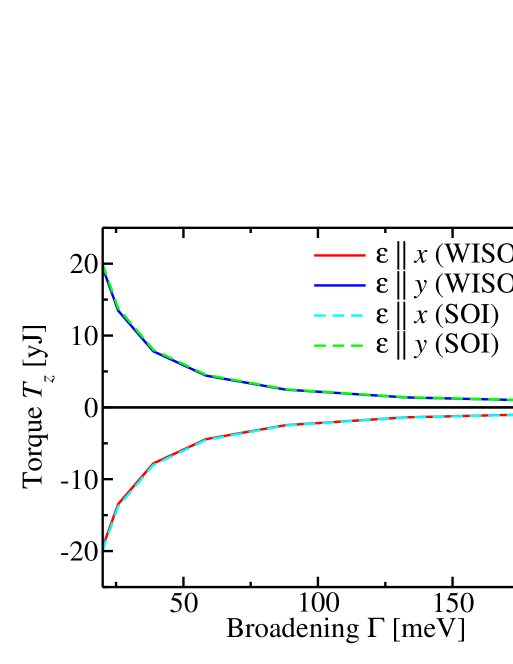
Figure 1: Laser-induced torque in Mn₂Au vs. quasi-particle broadening $\Gamma$ when the Néel vector points in the 110 direction. Comparison between the results obtained within the WISOI approach (solid lines) and the results obtained based on MLWFs that include SOI (dashed lines). The torque is shown in units of yJ=yoctojoule=10^-24Joule.

In this section we discuss laser induced torques for the laser intensity $I=10$ GW/cm² when the photon energy is set to 1.55 eV. In Fig. 1 we show the laser-induced torque as a function of $\Gamma$ when the Néel vector points in the 110 direction. This torque is consistent with tensor 4 in Table II.3, which describes a laser-induced torque in the $z$ direction that differs in sign for linearly polarized light along the $x$ and $y$ directions. The figure shows both the results obtained within the WISOI approach (solid lines) and the results obtained based on MLWFs that include SOI (dashed lines). The very good agreement between the two approaches proves the validity and accuracy of the WISOI approach. Therefore, all following figures below show only the WISOI results. In Fig. 1 we present the torque in units of yoctojoule. The effective staggered magnetic field that produces a torque of one yoctojoule is 14.5 mT. Thus, the torques shown in Fig. 1 are of the same order of magnitude as the laser-induced torques in the ferromagnets Fe, Co, and FePt that we studied in Ref. [11].

Tensor 4 predicts a torque in the $z$ direction also for light circularly polarized in the $yz$ or $zx$ planes. Our calculations confirm this prediction. For light circularly polarized in the $zx$ plane we find $T_{z}<0$ and its magnitude is half of the magnitude for linearly polarized light with ${\boldsymbol{\epsilon}}\|\hat{{\boldsymbol{e}}}_{x}$. Similarly, for light circularly polarized in the $yz$ plane we find $T_{z}$ to be half of what it is when ${\boldsymbol{\epsilon}}\|\hat{{\boldsymbol{e}}}_{y}$.

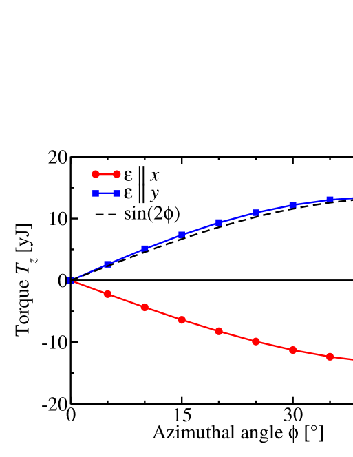
Figure 2: Laser-induced torque in Mn₂Au vs. azimuthal angle $\phi$ when the polar angle is $\theta=90^{\circ}$ and when $\Gamma=25$ meV.

In order to discuss the dependence of the laser-induced torque on the Néel vector we introduce the azimuthal angle $\phi$ and the polar angle $\theta$ such that $\hat{{\boldsymbol{\mathcal{L}}}}=(\sin\theta\cos\phi,\sin\theta\sin\phi,\cos\theta)^{\rm T}$. In Fig. 2 we show the laser-induced torque as a function of the azimuthal angle $\phi$ when $\theta=90^{\circ}$ and when the quasiparticle broadening is set to $\Gamma=25$ meV. Tensor 4 predicts the $\phi$ dependence $\propto\hat{M}_{x}\hat{M}_{y}\propto\sin\phi\cos\phi\propto\sin(2\phi)$, which is illustrated in Fig. 2 by the dashed line and which fits the ab-initio data very well.

In Fig. 3 we plot the component $T_{y}$ when the magnetization is along the $x$ direction and when ${\boldsymbol{\epsilon}}=(\hat{{\boldsymbol{e}}}_{x}+\hat{{\boldsymbol{e}}}_{z})/\sqrt{2}$ i.e., ${\boldsymbol{\epsilon}}\|(101)$. This torque is consistent with tensor 9, which predicts a torque in $y$ direction when the magnetization is along $x$ direction and when ${\boldsymbol{\epsilon}}$ lies in the $zx$ plane.

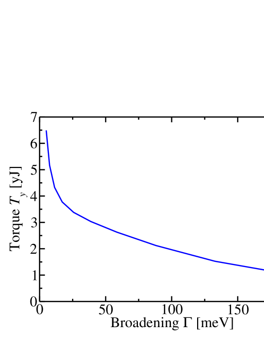
Figure 3: Laser-induced torque in Mn₂Au vs. quasi-particle broadening $\Gamma$ when the staggered magnetization is along (100), i.e., $\hat{{\boldsymbol{\mathcal{L}}}}=\hat{{\boldsymbol{e}}}_{x}$, and when ${\boldsymbol{\epsilon}}=(\hat{{\boldsymbol{e}}}_{x}+\hat{{\boldsymbol{e}}}_{z})/\sqrt{2}$, i.e., ${\boldsymbol{\epsilon}}\|(101)$.

Next, we discuss the case $\hat{{\boldsymbol{\mathcal{L}}}}=\hat{{\boldsymbol{e}}}_{z}$. In Fig. 4 we show $T_{y}$ for ${\boldsymbol{\epsilon}}=(\hat{{\boldsymbol{e}}}_{x}+\hat{{\boldsymbol{e}}}_{z})/\sqrt{2}$, i.e., ${\boldsymbol{\epsilon}}\|(101)$, and $T_{x}$ for ${\boldsymbol{\epsilon}}=(\hat{{\boldsymbol{e}}}_{y}+\hat{{\boldsymbol{e}}}_{z})/\sqrt{2}$ i.e., ${\boldsymbol{\epsilon}}\|(011)$. The torques $T_{x}$ and $T_{y}$ are equal but opposite in the figure, consistent with the tensor 17 in Table II.3.

Figure 4: Laser-induced torque in Mn₂Au vs. quasi-particle broadening $\Gamma$ when the staggered magnetization is along (001), i.e., $\hat{{\boldsymbol{\mathcal{L}}}}=\hat{{\boldsymbol{e}}}_{z}$.

III.3 Laser-induced torques at THz frequencies

In Fig. 5 we show the laser-induced torque for a THz-laser with frequency of 1 THz for the laser intensity $I=10$ GW/cm². The intensity $I=10$ GW/cm² corresponds to the electric field of the laser light of $E=2.7$ MV/cm. The SOT in Mn₂Au is described by the odd torkance $t^{\rm odd}=0.6ea_{0}$ at $\Gamma=25$ meV. The corresponding torque at $E=2.7$ MV/cm is 1370 yJ. This is larger than the maximum laser-induced torque in Fig. 5 by a factor of 2 only. At higher broadening $\Gamma=130$ meV we find a SOT of 230 yJ ($t^{\rm odd}=0.1ea_{0}$) and a laser-induced torque of 12 yJ. The ratio of SOT to the laser-induced torque is thus increased to a factor of 20 by the increase of broadening. At even higher broadening $\Gamma=200$ meV we find a SOT of 132 yJ ($t^{\rm odd}=0.058ea_{0}$) and a laser-induced torque of 2.6 yJ, i.e., the ratio of SOT to the laser-induced torque is further increased to 50.

In the experiment on CuMnAs in Ref. [19] it was shown that THz electric field pulses switch the Néel vector. This switching was attributed to the action of the SOT. We therefore compare the magnitudes of the SOT and of the laser-induced torque in Mn₂Au in order to judge if the laser-induced torque might contribute as well to the switching by THz pulses. In Ref. [19] the maximum amplitude of the applied THz electric field is $E=0.11$ MV/cm, which is smaller than $E=2.7$ MV/cm by a factor 24.5 and which corresponds to an intensity of 0.017 GW/cm² only. At such a small intensity the ratio of the SOT to the laser-induced torque is roughly 50 in Mn₂Au, such that the laser-induced torque is negligible in Mn₂Au already at $\Gamma=25$ meV. As discussed in the previous paragraph the ratio of the SOT to the laser-induced torque will futher increase by an order of magnitude when the broadening is increased to $\Gamma=130$ meV such that the contribution of the laser-induced torques relative to the SOT decreases even further with increasing broadening. Since the laser-induced torque scales quadratically with the electric field of the laser, it becomes more important relative to the SOT at higher fields. However, picosecond THz-pulses of intensities as high as $I=10$ GW/cm² are far above the damage threshold of CuMnAs.

While literature values for the damage threshold of Mn₂Au are not available, we assume that picosecond THz-pulses of intensities as high as $I=10$ GW/cm² cannot be applied to Mn₂Au without damaging it. In order to apply such high laser intensities without damaging the metallic AFMs much shorter femtosecond pulses are necessary. Therefore, we expect the SOTs from THz laser pulses to be more important than the laser-induced torques. However, when lasers with optical frequencies are used, the SOT oscillates with the frequency of the laser field, which is much higher than the AFM resonance frequencies and therefore the SOT cannot excite the AFM. Therefore, when lasers in the optical range are used the laser-induced torques are important while the SOT is irrelevant.

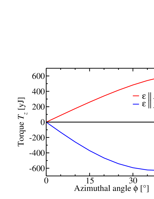
Figure 5: Laser-induced torque in Mn₂Au vs. azimuthal angle $\phi$ when the polar angle is $\theta=90^{\circ}$ and when $\Gamma=25$ meV.

IV Summary

We compute the laser-induced torques in the AFM Mn₂Au based on the Keldysh nonequilibrium approach. We find the laser-induced torques to be of the same order of magnitude as those in the ferromagnets Fe, Co, and FePt. From the phenomenological theory of the IFE in non-magnets one intuitively expects that laser-induced torques can be generated only by circularly polarized light. In contrast, we find that linearly polarized light is sufficient to stimulate torques in Mn₂Au. We corroborate this finding by a detailed symmetry analysis of the laser-induced torque. Additionally, we discuss the laser-induced torques at THz frequencies. At THz frequencies we compare the laser-induced torque to the SOT and find the SOT to be larger than the laser-induced torque by a factor of 50 at the light intensity used in experiments. In contrast, at optical frequencies only the laser-induced torque induces magnetization dynamics and the SOT may be neglected. In order to compute response coefficients from Wannier interpolation conveniently for many magnetization directions we develop the WISOI approach. We demonstrate that the WISOI approach reproduces the response coefficients obtained from MLWFs that include SOI with high accuracy.

Appendix A Spin-orbit coupling matrix elements

In this appendix we describe a procedure that allows us to use MLWFs that are calculated without SOI in order to compute material property tensors including the effect of SOI by adding the effect of SOI during the Wannier interpolation. The advantage of this procedure is that only two sets of MLWFs need to be calculated: One set of MLWFs for the spin-up states and a second set of MLWFs for the spin-down states.

We decompose the Hamiltonian as follows:

$$H=\bar{H}+\mathcal{V}_{\rm SOI},$$ (20)

where $\mathcal{V}_{\rm SOI}$ denotes SOI and $\bar{H}$ is the Hamiltonian without SOI. In order to obtain MLWFs without SOI, $\mathcal{V}_{\rm SOI}$ is ignored during the generation of MLWFs. We denote the MLWFs without SOI by $|\bar{W}_{{\boldsymbol{R}}n\sigma}\rangle$, where $\sigma=\uparrow,\downarrow$ labels the spin. The number of spin-up MLWFs is $N_{\uparrow}$ and the number of spin-down MLWFs is $N_{\downarrow}$. The total number of MLWFs is $N_{\rm W}=N_{\uparrow}+N_{\downarrow}$. The MLWFs are related to the Bloch functions by the transformation [27]

$$|\bar{W}_{{\boldsymbol{R}}n\sigma}\rangle=\frac{1}{\mathcal{N}}\sum_{{\boldsymbol{k}}}e^{-i{\boldsymbol{k}}\cdot{\boldsymbol{R}}}\sum_{m}U_{mn\sigma}^{({\boldsymbol{k}})}|\bar{\psi}_{{\boldsymbol{k}}m\sigma}\rangle,$$ (21)

where $\mathcal{N}$ is the number of ${\boldsymbol{k}}$-points used for the generation of the MLWFs and where the Bloch states $|\bar{\psi}_{{\boldsymbol{k}}m\sigma}\rangle$ are the eigenstates of the Hamiltonian $\bar{H}$ without SOI with corresponding eigenvalues $\bar{\mathcal{E}}_{{\boldsymbol{k}}n\sigma}$, i.e.,

$$\bar{H}|\bar{\psi}_{{\boldsymbol{k}}n\sigma}\rangle=\bar{\mathcal{E}}_{{\boldsymbol{k}}n\sigma}|\bar{\psi}_{{\boldsymbol{k}}n\sigma}\rangle.$$ (22)

The Wannier90 code [27] determines the transformation $U_{mn\sigma}^{({\boldsymbol{k}})}$ such that the resulting Wannier functions are maximally localized.

The Wannier-interpolated Hamiltonian matrix $\bar{{\boldsymbol{H}}}^{\rm W}_{{\boldsymbol{k}}}$ without SOI is given by the Fourier transform [27]

$$\bar{{\boldsymbol{H}}}^{\rm W}_{{\boldsymbol{k}}}=\begin{pmatrix}\bar{{\boldsymbol{h}}}^{\uparrow\uparrow}_{{\boldsymbol{k}}}&0\\ 0&\bar{{\boldsymbol{h}}}^{\downarrow\downarrow}_{{\boldsymbol{k}}}\end{pmatrix}=\sum_{{\boldsymbol{R}}}{\rm e}^{i{\boldsymbol{k}}\cdot{\boldsymbol{R}}}\begin{pmatrix}\bar{{\boldsymbol{h}}}^{\uparrow\uparrow}_{{\boldsymbol{R}}}&0\\ 0&\bar{{\boldsymbol{h}}}^{\downarrow\downarrow}_{{\boldsymbol{R}}}\end{pmatrix},$$ (23)

where $\bar{{\boldsymbol{h}}}^{\uparrow\uparrow}_{{\boldsymbol{k}}}$ and $\bar{{\boldsymbol{h}}}^{\uparrow\uparrow}_{{\boldsymbol{R}}}$ are $N_{\uparrow}\times N_{\uparrow}$-matrices and $\bar{{\boldsymbol{h}}}^{\downarrow\downarrow}_{{\boldsymbol{k}}}$ and $\bar{{\boldsymbol{h}}}^{\downarrow\downarrow}_{{\boldsymbol{R}}}$ are $N_{\downarrow}\times N_{\downarrow}$-matrices. $\bar{{\boldsymbol{H}}}_{{\boldsymbol{k}}}^{\rm W}$ is a $N_{\rm W}\times N_{\rm W}$-matrix. The matrix elements of $\bar{{\boldsymbol{h}}}^{\sigma\sigma}_{{\boldsymbol{R}}}$ are given by [27]

$$\bar{h}^{\sigma\sigma}_{{\boldsymbol{R}}nm} =\langle\bar{W}_{{\boldsymbol{0}}n\sigma}|\bar{H}|\bar{W}_{{\boldsymbol{R}}m\sigma}\rangle=$$ (24)

$$=\frac{1}{\mathcal{N}}\sum_{{\boldsymbol{k}}m^{\prime}}\bar{\mathcal{E}}_{{\boldsymbol{k}}m^{\prime}\sigma}e^{-i{\boldsymbol{k}}\cdot{\boldsymbol{R}}}\left(U^{({\boldsymbol{k}})}_{m^{\prime}n\sigma}\right)^{*}U_{m^{\prime}m\sigma}^{({\boldsymbol{k}})}.$$

Since SOI is important only close to the nuclei, we may neglect SOI in the interstitial regions between the atoms. We may therefore express SOI as

$$\mathcal{V}_{\rm SOI}=\sum_{\alpha}\xi_{\alpha}({\boldsymbol{r}}-{\boldsymbol{r}}_{\alpha}){\boldsymbol{L}}^{\alpha}\cdot{\boldsymbol{\sigma}},$$ (25)

where

$$\xi_{\alpha}({\boldsymbol{r}})=\left\{\begin{matrix}\frac{\mu_{\rm B}}{2cr}\frac{dV_{\alpha}(r)}{dr}{\rm\,\,for\,\,}|{\boldsymbol{r}}|<R_{\alpha}\\ 0{\rm\,\,for\,\,}|{\boldsymbol{r}}|>R_{\alpha}\end{matrix}\right.$$ (26)

is the SOI potential in a sphere around atom $\alpha$, $R_{\alpha}$ is the atomic radius of atom $\alpha$, ${\boldsymbol{r}}_{\alpha}$ is the position of the center of atom $\alpha$, ${\boldsymbol{L}}^{\alpha}=({\boldsymbol{r}}-{\boldsymbol{r}}_{\alpha})\times{\boldsymbol{p}}$ is the angular momentum operator of atom $\alpha$, and $V_{\alpha}(r)$ is the spherical part of the potential in the sphere around atom $\alpha$.

In order to add the effect of SOI the following matrix elements need to be evaluated in the basis of Bloch functions:

$$\mathcal{A}^{\sigma\sigma^{\prime}-}_{{\boldsymbol{k}}nm}=\sum_{\alpha}\langle\bar{\psi}_{{\boldsymbol{k}}n\sigma}|\xi_{\alpha}({\boldsymbol{r}}-{\boldsymbol{r}}_{\alpha})L^{\alpha}_{-}|\bar{\psi}_{{\boldsymbol{k}}m\sigma^{\prime}}\rangle,$$ (27)

$$\mathcal{A}^{\sigma\sigma^{\prime}+}_{{\boldsymbol{k}}nm}=\sum_{\alpha}\langle\bar{\psi}_{{\boldsymbol{k}}n\sigma}|\xi_{\alpha}({\boldsymbol{r}}-{\boldsymbol{r}}_{\alpha})L_{+}^{\alpha}|\bar{\psi}_{{\boldsymbol{k}}m\sigma^{\prime}}\rangle,$$ (28)

and

$$\mathcal{A}^{\sigma\sigma^{\prime}z}_{{\boldsymbol{k}}nm}=\sum_{\alpha}\langle\bar{\psi}_{{\boldsymbol{k}}n\sigma}|\xi_{\alpha}({\boldsymbol{r}}-{\boldsymbol{r}}_{\alpha})L_{z}^{\alpha}|\bar{\psi}_{{\boldsymbol{k}}m\sigma^{\prime}}\rangle,$$ (29)

where $L^{\alpha}_{+}=(L^{\alpha}_{x}+iL^{\alpha}_{y})$ and $L^{\alpha}_{-}=(L^{\alpha}_{x}-iL^{\alpha}_{y})$. These matrix elements satisfy the relations

$$\mathcal{A}^{\uparrow\uparrow z}_{{\boldsymbol{k}}mn}=\left[\mathcal{A}^{\uparrow\uparrow z}_{{\boldsymbol{k}}nm}\right]^{*}, \mathcal{A}^{\uparrow\uparrow+}_{{\boldsymbol{k}}mn}=\left[\mathcal{A}^{\uparrow\uparrow-}_{{\boldsymbol{k}}nm}\right]^{*},$$ (30)

$$\mathcal{A}^{\downarrow\downarrow z}_{{\boldsymbol{k}}mn}=\left[\mathcal{A}^{\downarrow\downarrow z}_{{\boldsymbol{k}}nm}\right]^{*}, \mathcal{A}^{\downarrow\downarrow+}_{{\boldsymbol{k}}mn}=\left[\mathcal{A}^{\downarrow\downarrow-}_{{\boldsymbol{k}}nm}\right]^{*},$$

$$\mathcal{A}^{\downarrow\uparrow z}_{{\boldsymbol{k}}mn}=\left[\mathcal{A}^{\uparrow\downarrow z}_{{\boldsymbol{k}}nm}\right]^{*}, \mathcal{A}^{\downarrow\uparrow+}_{{\boldsymbol{k}}mn}=\left[\mathcal{A}^{\uparrow\downarrow-}_{{\boldsymbol{k}}nm}\right]^{*}.$$

Subsequently, these matrix elements are transformed into the MLWF basis:

$$\mathcal{A}^{\sigma\sigma^{\prime}j}_{{\boldsymbol{R}}nm}=\sum_{\alpha}\langle\bar{W}_{{\boldsymbol{0}}n\sigma}|\xi_{\alpha}({\boldsymbol{r}}-{\boldsymbol{r}}_{\alpha})L_{j}^{\alpha}|\bar{W}_{{\boldsymbol{R}}m\sigma^{\prime}}\rangle$$ (31)

$$=\frac{1}{\mathcal{N}}\sum_{{\boldsymbol{k}}n^{\prime}m^{\prime}}e^{-i{\boldsymbol{k}}\cdot{\boldsymbol{R}}}[U^{({\boldsymbol{k}})}_{n^{\prime}n\sigma}]^{*}U^{({\boldsymbol{k}})}_{m^{\prime}m\sigma^{\prime}}\mathcal{A}^{\sigma\sigma^{\prime}j}_{{\boldsymbol{k}}n^{\prime}m^{\prime}},$$

where $j=-,z,+$.

When the (staggered) magnetization points into the direction $\hat{{\boldsymbol{\mathcal{L}}}}=(\sin\theta\cos\phi,\sin\theta\sin\phi,\cos\theta)^{\rm T}$ the spinor of the spin-up electrons is

$$|\uparrow,\theta,\phi\rangle=\left(\begin{array}[]{c}e^{-i\phi/2}\cos(\theta/2)\\ e^{i\phi/2}\sin(\theta/2)\end{array}\right)$$ (32)

while the spinor of the spin-down electrons is

$$|\downarrow,\theta,\phi\rangle=\left(\begin{array}[]{c}-e^{-i\phi/2}\sin(\theta/2)\\ e^{i\phi/2}\cos(\theta/2)\end{array}\right).$$ (33)

We define

$$\sigma_{+}=\sigma_{x}+i\sigma_{y},\quad\sigma_{-}=\sigma_{x}-i\sigma_{y}.$$ (34)

The matrix elements of $\sigma_{z}$ are

$$\langle\uparrow,\theta,\phi|\sigma_{z}|\uparrow,\theta,\phi\rangle=\cos\theta,$$ (35)

$$\langle\downarrow,\theta,\phi|\sigma_{z}|\downarrow,\theta,\phi\rangle=-\cos\theta,$$

$$\langle\uparrow,\theta,\phi|\sigma_{z}|\downarrow,\theta,\phi\rangle=-\sin\theta,$$

$$\langle\downarrow,\theta,\phi|\sigma_{z}|\uparrow,\theta,\phi\rangle=-\sin\theta.$$

The matrix elements of $\sigma_{+}$ are

$$\langle\uparrow,\theta,\phi|\sigma_{+}|\uparrow,\theta,\phi\rangle=\sin\theta{\rm e}^{i\phi},$$ (36)

$$\langle\downarrow,\theta,\phi|\sigma_{+}|\downarrow,\theta,\phi\rangle=-\sin\theta{\rm e}^{i\phi},$$

$$\langle\downarrow,\theta,\phi|\sigma_{+}|\uparrow,\theta,\phi\rangle=-2\left[\sin\frac{\theta}{2}\right]^{2}{\rm e}^{i\phi},$$

$$\langle\uparrow,\theta,\phi|\sigma_{+}|\downarrow,\theta,\phi\rangle=2\left[\cos\frac{\theta}{2}\right]^{2}{\rm e}^{i\phi}.$$

The matrix elements of $\sigma_{-}$ are

$$\langle\uparrow,\theta,\phi|\sigma_{-}|\uparrow,\theta,\phi\rangle=\sin\theta{\rm e}^{-i\phi},$$ (37)

$$\langle\downarrow,\theta,\phi|\sigma_{-}|\downarrow,\theta,\phi\rangle=-\sin\theta{\rm e}^{-i\phi},$$

$$\langle\downarrow,\theta,\phi|\sigma_{-}|\uparrow,\theta,\phi\rangle=2\left[\cos\frac{\theta}{2}\right]^{2}{\rm e}^{-i\phi},$$

$$\langle\uparrow,\theta,\phi|\sigma_{-}|\downarrow,\theta,\phi\rangle=-2\left[\sin\frac{\theta}{2}\right]^{2}{\rm e}^{-i\phi}.$$

The product ${\boldsymbol{L}}^{\alpha}\cdot{\boldsymbol{\sigma}}$ in Eq. (25) may be rewritten as ${\boldsymbol{L}}^{\alpha}\cdot{\boldsymbol{\sigma}}=L^{\alpha}_{z}\sigma_{z}+[L^{\alpha}_{+}\sigma_{-}+L^{\alpha}_{-}\sigma_{+}]/2$. Therefore, we need to multiply the matrix elements in Eq. (31) with the angular factors in Eq. (35), Eq. (36), and Eq. (37) in order to obtain the matrix elements of the SOI Hamiltonian Eq. (25) in the basis set of the MLWFs without SOI. The resulting matrix elements are given in Eq. (6), Eq. (7), Eq. (8), and Eq. (9) in the main text.

References

- Lambert et al. [2014] C.-H. Lambert, S. Mangin, B. S. D. C. S. Varaprasad, Y. K. Takahashi, M. Hehn, M. Cinchetti, G. Malinowski, K. Hono, Y. Fainman, M. Aeschlimann, and E. E. Fullerton, All-optical control of ferromagnetic thin films and nanostructures, Science 345, 1337 (2014).
- John et al. [2017] R. John, M. Berritta, D. Hinzke, C. Müller, T. Santos, H. Ulrichs, P. Nieves, J. Walowski, R. Mondal, O. Chubykalo-Fesenko, J. McCord, P. M. Oppeneer, U. Nowak, and M. Münzenberg, Magnetisation switching of fept nanoparticle recording medium by femtosecond laser pulses, Scientific Reports 7, 4114 (2017).
- Kimel et al. [2005] A. V. Kimel, A. Kirilyuk, P. A. Usachev, R. V. Pisarev, A. M. Balbashov, and T. Rasing, Ultrafast non-thermal control of magnetization by instantaneous photomagnetic pulses, Nature 435, 655 (2005).
- Nemec et al. [2012] P. Nemec, E. Rozkotova, N. Tesarova, F. Trojanek, E. De Ranieri, K. Olejnik, J. Zemen, V. Novak, M. Cukr, P. Maly, and T. Jungwirth, Experimental observation of the optical spin transfer torque, Nature physics 8, 411 (2012).
- Huisman et al. [2016] T. J. Huisman, R. V. Mikhaylovskiy, J. D. Costa, F. Freimuth, E. Paz, J. Ventura, P. P. Freitas, S. Blügel, Y. Mokrousov, T. Rasing, and A. V. Kimel, Femtosecond control of electric currents in metallic ferromagnetic heterostructures, Nature nanotechnology 11, 455 (2016).
- van Kampen et al. [2002] M. van Kampen, C. Jozsa, J. T. Kohlhepp, P. LeClair, L. Lagae, W. J. M. de Jonge, and B. Koopmans, All-optical probe of coherent spin waves, Phys. Rev. Lett. 88, 227201 (2002).
- Schellekens et al. [2014] A. J. Schellekens, K. C. Kuiper, R. R. J. C. de Wit, and B. Koopmans, Ultrafast spin-transfer torque driven by femtosecond pulsed-laser excitation, Nature Communications 5, 4333 (2014).
- Choi et al. [2015] G.-M. Choi, C.-H. Moon, B.-C. Min, K.-J. Lee, and D. G. Cahill, Thermal spin-transfer torque driven by the spin-dependent Seebeck effect in metallic spin-valves, Nature physics 11, 576 (2015).
- Capua et al. [2017] A. Capua, C. Rettner, S.-H. Yang, T. Phung, and S. S. P. Parkin, Ensemble-averaged Rabi oscillations in a ferromagnetic film, NATURE COMMUNICATIONS 8, 16004 (2017).
- Choi et al. [2017] G.-M. Choi, A. Schleife, and D. G. Cahill, Optical-helicity-driven magnetization dynamics in metallic ferromagnets, Nature Communications 8, 15085 (2017).
- Freimuth et al. [2016] F. Freimuth, S. Blügel, and Y. Mokrousov, Laser-induced torques in metallic ferromagnets, Phys. Rev. B 94, 144432 (2016).
- Baláž et al. [2020] P. Baláž, K. Carva, U. Ritzmann, P. Maldonado, and P. M. Oppeneer, Domain wall dynamics due to femtosecond laser-induced superdiffusive spin transport, Phys. Rev. B 101, 174418 (2020).
- Ritzmann et al. [2020] U. Ritzmann, P. Baláž, P. Maldonado, K. Carva, and P. M. Oppeneer, High-frequency magnon excitation due to femtosecond spin-transfer torques, Phys. Rev. B 101, 174427 (2020).
- Qaiumzadeh and Titov [2016] A. Qaiumzadeh and M. Titov, Theory of light-induced effective magnetic field in rashba ferromagnets, Phys. Rev. B 94, 014425 (2016).
- Berritta et al. [2016] M. Berritta, R. Mondal, K. Carva, and P. M. Oppeneer, Ab initio theory of coherent laser-induced magnetization in metals, Phys. Rev. Lett. 117, 137203 (2016).
- Baltz et al. [2018] V. Baltz, A. Manchon, M. Tsoi, T. Moriyama, T. Ono, and Y. Tserkovnyak, Antiferromagnetic spintronics, Rev. Mod. Phys. 90, 015005 (2018).
- Manchon et al. [2019] A. Manchon, J. Železný, I. M. Miron, T. Jungwirth, J. Sinova, A. Thiaville, K. Garello, and P. Gambardella, Current-induced spin-orbit torques in ferromagnetic and antiferromagnetic systems, Rev. Mod. Phys. 91, 035004 (2019).
- Gomonay and Loktev [2014] E. V. Gomonay and V. M. Loktev, Spintronics of antiferromagnetic systems (review article), Low Temperature Physics 40, 17 (2014).
- Olejník et al. [2018] K. Olejník, T. Seifert, Z. Kašpar, V. Novák, P. Wadley, R. P. Campion, M. Baumgartner, P. Gambardella, P. Němec, J. Wunderlich, J. Sinova, P. Kužel, M. Müller, T. Kampfrath, and T. Jungwirth, Terahertz electrical writing speed in an antiferromagnetic memory, Science Advances 4, 10.1126/sciadv.aar3566 (2018).
- Železný et al. [2014] J. Železný, H. Gao, K. Výborný, J. Zemen, J. Mašek, A. Manchon, J. Wunderlich, J. Sinova, and T. Jungwirth, Relativistic néel-order fields induced by electrical current in antiferromagnets, Phys. Rev. Lett. 113, 157201 (2014).
- Železný et al. [2017] J. Železný, H. Gao, A. Manchon, F. Freimuth, Y. Mokrousov, J. Zemen, J. Mašek, J. Sinova, and T. Jungwirth, Spin-orbit torques in locally and globally noncentrosymmetric crystals: Antiferromagnets and ferromagnets, Phys. Rev. B 95, 014403 (2017).
- Salemi et al. [2019] L. Salemi, M. Berritta, A. K. Nandy, and P. M. Oppeneer, Orbitally dominated rashba-edelstein effect in noncentrosymmetric antiferromagnets, Nature Communications 10, 5381 (2019).
- Bodnar et al. [2018] S. Y. Bodnar, L. Šmejkal, I. Turek, T. Jungwirth, O. Gomonay, J. Sinova, A. A. Sapozhnik, H. J. Elmers, M. Kläui, and M. Jourdan, Writing and reading antiferromagnetic by néel spin-orbit torques and large anisotropic magnetoresistance, Nature Communications 9, 348 (2018).
- Meinert et al. [2018] M. Meinert, D. Graulich, and T. Matalla-Wagner, Electrical switching of antiferromagnetic and the role of thermal activation, Phys. Rev. Applied 9, 064040 (2018).
- Zhou et al. [2018] X. F. Zhou, J. Zhang, F. Li, X. Z. Chen, G. Y. Shi, Y. Z. Tan, Y. D. Gu, M. S. Saleem, H. Q. Wu, F. Pan, and C. Song, Strong orientation-dependent spin-orbit torque in thin films of the antiferromagnet , Phys. Rev. Applied 9, 054028 (2018).
- Bodnar et al. [2019] S. Y. Bodnar, M. Filianina, S. P. Bommanaboyena, T. Forrest, F. Maccherozzi, A. A. Sapozhnik, Y. Skourski, M. Kläui, and M. Jourdan, Imaging of current induced éel vector switching in antiferromagnetic , Phys. Rev. B 99, 140409(R) (2019).
- Pizzi et al. [2020] G. Pizzi, V. Vitale, R. Arita, S. Blügel, F. Freimuth, G. Géranton, M. Gibertini, D. Gresch, C. Johnson, T. Koretsune, and et al., Wannier90 as a community code: new features and applications, J. Phys.: Condens. Matter 32, 165902 (2020).
- Battiato et al. [2012] M. Battiato, G. Barbalinardo, K. Carva, and P. M. Oppeneer, Beyond linear response theory for intensive light-matter interactions: Order formalism and ultrafast transient dynamics, Phys. Rev. B 85, 045117 (2012).
- Freimuth et al. [2021] F. Freimuth, S. Blügel, and Y. Mokrousov, Charge and spin photocurrents in the rashba model, Phys. Rev. B 103, 075428 (2021).
- Kraut and von Baltz [1979] W. Kraut and R. von Baltz, Anomalous bulk photovoltaic effect in ferroelectrics: A quadratic response theory, Phys. Rev. B 19, 1548 (1979).
- von Baltz and Kraut [1981] R. von Baltz and W. Kraut, Theory of the bulk photovoltaic effect in pure crystals, Phys. Rev. B 23, 5590 (1981).
- Zhang et al. [2018] Y. Zhang, H. Ishizuka, J. van den Brink, C. Felser, B. Yan, and N. Nagaosa, Photogalvanic effect in weyl semimetals from first principles, Phys. Rev. B 97, 241118(R) (2018).
- Go et al. [2020] D. Go, F. Freimuth, J.-P. Hanke, F. Xue, O. Gomonay, K.-J. Lee, S. Blügel, P. M. Haney, H.-W. Lee, and Y. Mokrousov, Theory of current-induced angular momentum transfer dynamics in spin-orbit coupled systems, Phys. Rev. Research 2, 033401 (2020).
- Ding et al. [2020] S. Ding, A. Ross, D. Go, L. Baldrati, Z. Ren, F. Freimuth, S. Becker, F. Kammerbauer, J. Yang, G. Jakob, Y. Mokrousov, and M. Kläui, Harnessing orbital-to-spin conversion of interfacial orbital currents for efficient spin-orbit torques, Phys. Rev. Lett. 125, 177201 (2020).
- Tazaki et al. [2020] Y. Tazaki, Y. Kageyama, H. Hayashi, T. Harumoto, T. Gao, J. Shi, and K. Ando, Current-induced torque originating from orbital current (2020), arXiv:2004.09165 [cond-mat.mtrl-sci] .
- Kim et al. [2021] J. Kim, D. Go, H. Tsai, D. Jo, K. Kondou, H.-W. Lee, and Y. Otani, Nontrivial torque generation by orbital angular momentum injection in ferromagnetic-metal/ trilayers, Phys. Rev. B 103, L020407 (2021).
- Johansson et al. [2021] A. Johansson, B. Göbel, J. Henk, M. Bibes, and I. Mertig, Spin and orbital edelstein effects in a two-dimensional electron gas: Theory and application to interfaces, Phys. Rev. Research 3, 013275 (2021).
- [38] See http://www.flapw.de.
- Perdew et al. [1996] J. P. Perdew, K. Burke, and M. Ernzerhof, Generalized gradient approximation made simple, Phys. Rev. Lett. 77, 3865 (1996).
- Wells and Smith [1970] P. Wells and J. H. Smith, The structure of and , Acta Crystallographica Section A 26, 379 (1970).
- Freimuth et al. [2008] F. Freimuth, Y. Mokrousov, D. Wortmann, S. Heinze, and S. Blügel, Maximally localized Wannier functions within the FLAPW formalism, Phys. Rev. B 78, 035120 (2008).