Venus upper atmosphere revealed by a GCM: II. Model validation with temperature and density measurements

Abstract

An improved high resolution (96 longitude by 96 latitude points) ground-to-thermosphere version of the Institut Pierre-Simon Laplace (IPSL) Venus General Circulation Model (VGCM), including non-orographic gravity waves (GW) parameterization and fine-tuned non-LTE parameters, is presented here. We focus on the validation of the model built from a collection of data mostly from Venus Express (2006-2014) experiments and coordinated ground-based telescope campaigns, in the upper mesosphere/lower thermosphere of Venus (80-150 km). These simulations result in an overall better agreement with temperature observations above 90 km, compared with previous versions of the VGCM. Density of CO₂ and light species, such as CO and O, are also comparable with observations in terms of trend and order of magnitude. Systematic biases in the temperature structure are found between 80 and 100 km approximately (e.g. GCM is 20 to 40 K warmer than measurements) and above 130 km at the terminator (e.g. GCM is up to 50 K colder than observed). Possible candidates for those discrepancies are the uncertainties on the collisional rate coefficients used in the non-LTE parameterization (above 130 km), and assumptions on the CO₂ mixing ratio made for stellar/solar occultation retrievals. Diurnal and latitudinal distribution of dynamical tracers (i.e. CO and O) are also analyzed, in a region poorly constrained by wind measurements and characterized by high variability over daily to weekly timescale. Overall, our simulations indicate that a weak westward retrograde wind is present in the mesosphere, up to about 120 km, producing the CO bulge displacement toward 2h-3h in the morning, instead of piling up at the anti-solar point, as for an idealized sub-solar to anti-solar circulation. This retrograde imbalance is suggested to be produced by perturbations of a $\sim$ 5 days Kelvin wave impacting the mesosphere up to 110 km (described in the companion paper Navarro et al. [2021]), combined with GW westward acceleration in the lower thermosphere, mostly above 110 km. On the whole, these model developments point to the importance of the inclusion of the lower atmosphere, higher resolution and finely tuned parameterizations in GCM of the Venusian upper atmosphere, in order to shed light on existing observations.

1 Introduction

Our understanding of the Venusian climate has noticeably increased with progress with General Circulation Models (GCM), powerful 3D tools to investigate the amount of data acquired by space missions, particularly in recent time by Venus Express (VEx) [e.g Drossart et al., 2007a, Piccioni et al., 2007] and Akatsuki [e.g Satoh et al., 2017, Fukuhara et al., 2017] missions, as well as on-going ground-based telescope campaigns. For instance, some model experiments agree on the role of thermal tides in the vertical transport of angular momentum in the equatorial region and in maintaining the superrotation [Yamamoto and Takahashi, 2006, Takagi and Matsuda, 2007, Lebonnois et al., 2010, Mendonça and Read, 2016, Yamamoto et al., 2021]. Others succeeded to reproduce the polar atmospheric structure and the “cold collar” [Ando et al., 2016, Garate-Lopez and Lebonnois, 2018], in close agreement with the observations, in particular when the latitudinal variations of the cloud structure are taken into account.

Despite numerous and increasing observations, our view of the upper mesosphere and lower thermosphere (UMLT) of Venus (i.e. 80 km-140 km approximately) still remains incomplete. Therefore, GCMs are also used to understand the atmospheric conditions of high altitude regions where some key observations are lacking, especially on the dayside [Brecht and Bougher, 2012, Gilli et al., 2017]. The UMLT is characterized by strong diurnal variations in atmospheric temperatures which drive Subsolar-to-Antisolar (SS-AS) transport of photolyzed products such as CO, O, NO, H, O₂ singlet delta, toward strong nighttime enhancements in the thermosphere [Clancy et al., 2012].

VEx observations (2006-2014) revealed an even more variable atmosphere than expected: in particular, the so-called “transition” region ($\sim$ 80-120 km), between the retrograde superrotating zonal (RSZ) flow and the day-to-night circulation, showed latitude and day-to-day variations of temperature up to 80 K above 100 km at the terminator, and apparent zonal wind velocities measured around 96 km on the Venus nighttime highly changing in space and time. Current 3D models do not fully explain those variations, and specific processes (e.g. gravity wave propagation, thermal tides, large scale planetary waves) responsible for driving them are still under investigation.

However, it is difficult to simulate all individual wave sources of temporal and spatial variability observed within the Venus atmosphere due to resolution constraints. It is useful for a modeling approach to have a more extensive collection of measurements to provide statistical means. An example of a comprehensive data inter-comparison is the work presented in Limaye et al. [2017] (hereinafter Limaye17), showing the state-of-the-art temperature and total density measurements taken during VEx lifetime by instruments onboard and by ground-based telescopes. The study by Limaye17 put in evidence that, although there is a generally good agreement between the various experiments, differences between individual experiments are more significant than measurement uncertainties, especially above 100 km, revealing a considerable temperature variability. These experiments observed the Venus atmosphere’s vertical and latitudinal temperature structure, unveiling features that appear to be systematically present, such as a succession of warm and cold layers.
Regarding abundances of tracers in the UMLT, Vandaele et al. [2016] reported retrievals of CO spanning the 65-150 km altitude range during the whole VEx mission with the instrument SOIR (Solar Occultation in the InfraRed) together with an updated comparison of CO measurements from the literature. Within the high variability observed in the short term, reaching one order of magnitude on less than one month period, they also found a systematic latitudinal trend: CO abundances in the equatorial region were larger than high-latitude (60^∘-80^∘) and polar (80^∘-90^∘) abundances by a factor 2 and 3 respectively at an altitude of 130 km. However, below 100 km, the trend is reversed (i.e., equator-to-pole increasing), as reported by previous observations [Irwin et al., 2008, Marcq et al., 2015]. This trend reversion supports the existence of a Hadley cell circulation type [Taylor, 1995, Taylor and Grinspoon, 2009, Tsang et al., 2008, Marcq et al., 2015]. Interestingly, the density profiles measured by SOIR on board VEx showed a distinctive change of slope with altitude occurring in the region usually lying between 100-110 km altitude, also present in the Venus International Reference Atmosphere (VIRA) model, but at a lower altitude [Vandaele et al., 2016]. In VIRA, this may be caused by different observations feeding the model for CO: above 100 km, VIRA data is based on measurements reported by Keating et al. [1985], below 100 km the values are those reported by von Zahn et al. [1983] and later updated by de Bergh et al. [2006] and Zasova et al. [2006]. Simultaneous CO and temperature measurements in the lower thermosphere [Clancy et al., 2012] suggested instead that a distinctive circulation pattern would force large-scale air masses downward, creating dynamic increases in temperature and CO mixing ratio. SOIR evening abundances are also systematically higher than morning values above 105 km altitude, but the reverse is observed at lower altitudes.

Regarding the wind, the most relevant constraints in the mesosphere/thermosphere are provided by the diurnal/meridional distribution of CO and of the O₂ 1.27 $\mu$m IR nightglow, whose peak emission occurs at 96 $\pm$ 1 km in limb viewing [Drossart et al., 2007b]. Both CO and O are produced by CO₂ photo-dissociation during daytime and then transported to the nightside by the SS-AS circulation. Light species like CO are expected to pile up at the converging stagnation point of the wind field (i.e., the point where the horizontal velocity converges to zero). This stagnation point is at the anti-solar point for idealized SS-AS flow and displaced toward the morning terminator when a westward retrograde zonal flow is added. The position of the maximum and its magnitude depend on the relative values of equatorial velocity and a maximum cross-terminator velocity. Lellouch et al. [2008] observations showed a moderate (factor 2) CO enhancement near the morning terminator. To first order, this picture should be valid for the O₂ airglow. However, the situation is somewhat more complex in this case because the brightness of the O₂ emission also depends on chemistry and vertical transport (see companion paper by Navarro et al. [2021], hereinafter Navarro21).
In addition, a combination of nightside and terminator Doppler CO wind measurements took advantage of a rare solar transit in June 2012 to address several important questions regarding Venus’s upper atmospheric dynamics. Moullet et al. [2012] found a substantial nightside retrograde zonal wind field near the equator, also detected in other nightside distribution studies and less pronounced in the dayside lower thermospheric circulation [Clancy and Muhleman, 1991, Gurwell et al., 1995, Lellouch et al., 2008, Clancy et al., 2012]. This was interpreted as the presence of weaker morning versus evening cross-terminator winds, likely to be associated with morning-evening asymmetric momentum drag due to enhanced gravity wave (GW) absorption over the morning thermospheric region [Alexander et al., 1992, Bougher et al., 2006, Clancy et al., 2015]. Model simulations in Hoshino et al. [2013] showed that gravity wave forcing, coupled with a 40 m/s westward retrograde zonal wind field at 80 km altitude, is sufficient to impart a strong morning-evening asymmetry, as observed apart from the observed extreme temporal variability. Clancy et al. [2015] also measured substantially weaker morning terminator winds compared with evening terminator, consistent with Hoshino et al. [2013] results. However, the theoretical basis for forcing this asymmetry and associated retrograde zonal flow is not provided yet. Overall, wind distributions during nightside show much larger changes (50-100 m/s) over timescales of days to weeks than dayside winds [Clancy et al., 2015].

Despite observational and modeling efforts in the last decades, Venusian upper atmosphere’s temperature structure and dynamical behavior still raise questions: what are the sources of the variability observed in the airglow emissions on the nightside? Solar flux variation is expected to play only a minor role in the rapid changes observed in the nightglow morphological distribution [Gérard et al., 2014, 2017]. Instead, gravity waves have been suggested as a source of variability but have not been demonstrated to provide the required amplitude. In the companion article Navarro21, the state-of-the-art Venus GCM developed at the Institut Pierre-Simon Laplace (IPSL-VGCM) is used as well to investigate the variability of the upper atmosphere caused by a Kelvin wave generated in the cloud deck reaching the UMLT, and a supersonic shock-like structure wave in the thermosphere. In this paper, this same version of the IPSL-VGCM is validated with the most recent literature on observations of Venus UMLT atmospheric region, focusing on temperature, CO₂, CO and O abundances, and the effect of propagating non-orographic GW on those abundances is discussed.

Section 2 contains the description of the state-of-the-art of the IPSL-VGCM. The details on the formalism adopted for the non-orographic GW parameterization, with the GW parameters setup, and the improvement of non-LTE parameterization are in Appendices A and B. In this work, the outputs of the simulations obtained with the current high-resolution version (as Navarro21) are compared with a selection of data in Section 3, while an analysis of predicted diurnal and latitudinal variations of O and CO is presented in Section 4. The results are further discussed in Section 5 and the possible effects of propagating GW to the predicted abundances analyzed. Section 6 is focused on conclusive remarks and recommendations for future studies.

2 Model description and recent improvements

The IPSL Venus GCM (IPSL-VGCM) has been used to investigate all regions of the Venusian atmosphere, as it covers the surface up to the thermosphere (150 km) [Lebonnois et al., 2016, Gilli et al., 2017, Garate-Lopez and Lebonnois, 2018, Navarro et al., 2018]. The vertical model resolution is approximately $\sim$ 2-3 km between 100 and 150 km, slightly smaller below 100 km. It includes a non-orographic GW parameterization as described in details in the A, and a photochemical module with a simplified cloud scheme, with fixed bi-modal log-normal distribution of the cloud varying with altitude. The aerosol number density is calculated for each mode and an explicit description of the H₂O and H₂SO₄ mixing ratios in the liquid phase is included. The mass sedimentation flux is added to tracers evolution, but the microphysical scheme is not coupled with dynamics. The evaluated mass loading in the cloud is not used by the radiative module which instead use a scheme recently updated in Garate-Lopez and Lebonnois [2018]. That takes into account the latitudinal variation of the cloud structure based on Venus Express observations, and lower haze heating rate yielding to a better agreement with in-situ values of wind below the cloud deck (around 45 km altitude) by the Pioneer Venus probes [Schubert, 1983]. Chemical abundances play a crucial role in non-LTE effects (e.g., the impact of variable atomic O in the CO₂ cooling rates) and EUV heating processes, which are key processes in the upper atmosphere of terrestrial planets [Bougher et al., 1999]. Our model is currently the only GCM coupled with photochemistry, which enables the study of the upper atmosphere and its composition self-consistently [Stolzenbach, 2016, ; Stolzenbach et al. in preparation]. Here we followed the same approach as in Gilli17: the molecular weigh is calculated up to 150 km according to the chemical composition of the atmosphere, and the homopause level is evaluated by the GCM. The potential impact of a variable composition below 100 km, as revealed by N₂ concentration measurements between 60 and 100 km of 40 $\%$ higher than the nominal value [Peplowski et al., 2020] was not taken into account in this study, since we estimate that it would have a negligible impact on our results. Note that the IPSL-VGCM considers only neutral species so far, but future developments will be addressed to extend the model up to the exobase of Venus ($\sim$ 250 km altitude) and take into account the ionospheric chemistry. Moreover, the inclusion of a stochastic non-orographic gravity wave parameterization is a plus compared to other existent thermospheric models [Brecht and Bougher, 2012, Bougher et al., 2015] which accomplished deceleration of supersonic cross terminator winds artificially by Rayleigh friction.

2.1 Recent improvements

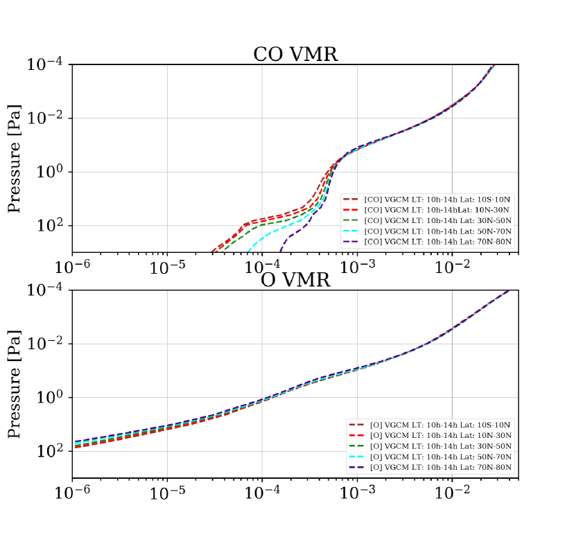
Figure 12: Latitudinal variations of CO and O vmr during daytime (10h-14h) predicted by the IPSL-VGCM. The latitude bins are indicated in each panel. The pressure levels correspond to an altitude range between 75 and 140 km, approximately. CO profiles show a clear transition of regime at around 1 Pa (100-110 km)

Compared with the previous ground-to-thermosphere VGCM described in Gilli et al. [2017] (hereinafter Gilli17), we include here several improvements in both radiative transfer code and non-LTE parameterization. The details of the improved non-LTE parameterization are provided in B. Also, we increased the horizontal resolution from 7.5${}^{\circ}\times$5.625^∘ to 3.75${}^{\circ}\times$1.875^∘ resulting in qualitative changes of the UMLT nighttime circulation dynamics, as explained in Navarro21. The predicted thermal structure presented in Gilli17 already captured a succession of warm and cold layers, as observed by VEx, but localized data-model discrepancies suggested model improvements. At the terminator and at nighttime thermospheric temperatures were about 40–50 K colder and up to 30 K warmer, respectively. The altitude layer of the predicted mesospheric local maximum (between 100 and 120 km) was also higher than observed, and systematically warmer, indicating an overestimation of daytime heating rates produced by absorption of IR solar radiation by CO₂ molecules. Among several sources of discrepancies, we identified one possible candidate. First, we discarded the effect of the uncertainty in the collisional rate coefficient K_v-t used in the non-LTE parameterization because, as shown in Figure 12 in Gilli17, the variation associated with this coefficient only modified the temperature profiles in the thermosphere above $10^{-2}$ Pa (about 120 km), not below. We focused instead on the heating rate used as “reference” in Gilli17, extracted from non-LTE radiative transfer line-by-line model results in [Roldán et al., 2000]. In that model, the kinetic temperature and density input profiles were taken from VIRA [Keating et al., 1985, Hedin et al., 1983]. Nevertheless, VEx observations revealed that VIRA is not representative of the atmosphere of Venus above 90 km [Limaye et al., 2017]. VIRA is based on Pioneer Venus measurements below 100 km and above 140 km, leaving a gap where the empirical models perform poorly [Bougher et al., 2015]. New measurements of the thermal structure of the Venusian atmosphere offer the opportunity to improve these empirical models. Therefore, we decided to perform here a semi-empirical fine-tuning of the non-LTE parameterization implemented in Gilli17, based on temperature profiles by SOIR and SPICAV, as described in the next session. Note that we first performed baseline simulations with a less computationally intensive version (i.e. low horizontal resolution version 7.5^∘ x 5.625^∘ as in Gilli17). Successively, we increased the horizontal resolution to 3.75^∘ x 1.875^∘, without significant changes in the heating/cooling rates above 90 km. The combination of this high horizontal resolution and a more realistic representation of zonal winds [Garate-Lopez and Lebonnois, 2018] and temperature gave rise to a very unique GCM, able to describe the circulation of the upper atmosphere of Venus with unprecedented details, as described in the companion paper Navarro21.

Parameter description	Best-Fit	Gilli17
Solar Heating per Venusian day, $Vd$ [$Kday^{-1}$]	15.92	18.13
Cloud top pressure level, $p_{0}$ [$Pa$]	1985	1320
Pressure below which non-LTE are significant, $p_{1}$ [$Pa$]	0.1	0.008
Central Pressure for LTE non-LTE transition, $ptrans$ [$Pa$]	0.2	0.5

Table 1: ”Best-fit” values from the improved non-LTE parameterization used in this work, compared with previous version in Gilli17. See Appendix B for details.

2.2 Fine-tuning of non-LTE parameters

In order to fine-tune and select the set of “best-fit” parameters listed in Table 1 we performed about 100 GCM test simulations with the goal of reducing as best as possible the discrepancies found between the averaged temperature profiles of the IPSL-VGCM and VEx dataset, in particular with SOIR/VEx [Mahieux et al., 2012] and SPICAV/VEx [Piccialli et al., 2014] profiles at the terminator and at night time, respectively. The major difficulty of this fine-tuning exercise was to find a combination of parameters described in B which also fulfills model numerical stability requirements (e.g. that allowed to run the model for several Venus days). The range of parameters that have been tested in this fine-tuning exercise is: 15.576 K to 24.60 K/day for the Solar heating per Venusian day, 1200 to 4350 Pa for the cloud-top pressure level, 6$\times 10^{-3}$ to 2.4 Pa for the pressure below which non-LTE effects are significant, and from 0.10 to 5 Pa for the center of the transition between non-LTE and LTE regime. The collisional rate coefficient was not changed compared to Gilli17. It is fixed at 3$\times 10^{-12}$, that is a ”median” value commonly used in terrestrial atmosphere models.

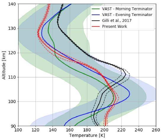
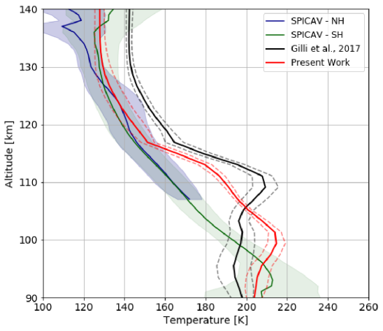
Figure 1: Averaged temperature vertical profiles as function of altitude predicted by the IPSL-VGCM before (solid black line) and after (solid red line) improving the non-LTE parameterization, together with observational data from Venus Express. Top panel: temperature retrieval results at the terminator (green for morning and blue for evening terminator) at the latitude bin 30ºN-60ºN extracted from the Venus Atmosphere from SOIR data at the Terminator (VAST) database [Mahieux et al., 2015]. SOIR standard deviation is also plotted as shaded green and blue areas. Bottom panel: Temperature retrieval results from SPICAV/VEx for the Northern Hemisphere (SPICAV - NH), 30ºN-50ºN in dark blue, and for the Southern Hemisphere (SPICAV - SH), 30ºS-50ºS in green (after Piccialli et al. [2015]). Standard deviation of the predicted temperature mean, in the same local time and latitude range as observed, is represented by dashed lines.

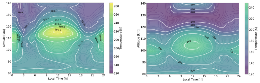
Figure 2: Temperature field (local time versus altitude) obtained with IPSL-VGCM before (left panel) and after (right panel) the non-LTE parameterization improvements, listed in Table 1.

Figure 1 shows an example of this improvement. Predicted upper mesospheric temperature (above 110 km approximately) are noticeably reduced by 20 K compared with the previous IPSL-VGCM version in Gilli17, and both the intensity and the altitude of the warm layer around 100 km are in better agreement with SOIR profiles. At nighttime the agreement is improved above 100 km with colder simulated temperature by 20 K, closer to observations. Above approximately 115 km, GCM results are within SPICAV error bars, though there are still data-model differences of about 20 K in the region between 100 and 115 km. The peak observed around 90-95 km is still higher in the model (around 100 km), despite a significant improvement. A detailed comparison of IPSL-VGCM results with a number of temperature measurements by VEx and ground-based experiments is provided in the next section. Temperature cross section (local time versus altitude) before and after the improvement of non-LTE parameterization is shown in Figure 2. The peak of temperature around midday and midnight is reduced by about 40 K and 20 K, respectively, and it is located about 10 km lower than predicted in Gilli17 (e.g. around 105 km and 100 km at midday and midnight, respectively). The temperature structure predicted by the IPSL-VGCM used in this work is in better agreement not only with VEx observations (see next section), but also with the National Center for Atmospheric Research (NCAR) Venus Thermospheric General Circulation Model presented in Brecht and Bougher [2012] (see their Figure 1).

3 IPSL-VGCM high resolution simulations: model-data validation above 90 km

The results discussed from this section onwards were performed using high horizontal resolution (96$\times$96$\times$78) simulations of the state-of-the-art IPSL-VGCM described in section 2. This is the highest resolution ever used for a Venus upper atmosphere model, corresponding to grid cells of approximately 200 km in the meridional direction and 400 km in the zonal direction, at the equator. This increased resolution allows to resolve smaller-scale waves compared to those in Gilli et al. [2017] and to shed a light on the observed variability in the nightside of Venus (see Navarro21). We aim to present an exhaustive data-model comparison with the state-of-the-art IPSL-VGCM, focusing on the atmospheric layers above 85-90 km, using the most complete compilation of Venus temperature and CO₂ density dataset so far, obtained both from space mission and ground based observations as in Limaye2017. Moreover, a selection of CO retrieved measurements by SOIR/VEx at the terminator [Vandaele et al., 2016], by VIRTIS/VEx during daytime [Gilli et al., 2015] and from Earth-based telescopes [Clancy et al., 2012] are considered here. For the atomic oxygen, only indirect O nighttime densities retrieved from O₂ nightglows as in Soret et al. [2012] are available for this comparison exercise. The instruments and measurements used in this validation exercise are listed in Table 2.

Experiment/Instrument	Method	Lat Coverage	LT Coverage	Alt Coverage	Retrieved variable	References
Remote sensing observations
from spacecraft
Magellan	Radio occultation	N/S hemisphere	night/day side	38-100 km	Temperature	Jenkins et al. [1994]
Venera 15	Radio occultation	N/S hemisphere	night/day side	38-100 km	Temperature	Gubenko et al. [2008], Haus et al. [2013]
Pioneer Venus	Radio occultation	N/S hemisphere	night/day side	38-100 km	Temperature	Kliore [1985], Seiff et al. [1985]
VeRa/VEx	Radio occultation	N/S hemisphere	night/day side	38-100 km	Temperature, CO2	Tellmann et al. [2009]
SPICAV/VEx	Stellar occultation	N/S hemisphere	night side	90-140 km	Temperature, CO2	Piccialli et al. [2010]
SOIR/VEx	Solar occultation	N/S hemisphere	terminators	70-170 km	Temperature, CO2, CO	Mahieux et al. [2010], Vandaele et al. [2016]
VIRTIS-H/VEx Limb	non-LTE 4.7 $\mu$m CO band	N hemisphere	day side	100-150 km	Temperature, CO	Gilli et al. [2015]
VIRTIS-H/VEx	4.3 $\mu$m CO2 band	N/S hemisphere	night side	65-80 km	Temperature	Migliorini et al. [2012]
VIRTIS-M/VEx Nadir	4.3 $\mu$m CO2 band	N/S hemisphere	night side	65-80 km	Temperature	Haus et al. [2013], Grassi et al. [2014]
VIRTIS-M/VEX	O2 nightglow at 1.27 $\mu$m	N/S hemisphere	night side	$\sim$ 96 km	O	Soret et al. [2012]
VExADE-AER/VEX	Aerobraking	70∘N-80∘N	morning terminator	130-140 km	CO2	Müller-Wodarg et al. [2016]
VExADE-TRQ/VEX	Torque measurements	70∘N-80∘N	78-98∘ SZA	165-200 km	CO2	Persson [2015]
HMI/SDO	Venus transit	N/S hemisphere	Terminator	70-110 km	Temperature	Tanga et al. [2012], Pere et al. [2016]
Ground-based observations
THIS/HIPWAC	non-LTE CO2 emission	N/S hemisphere	day side	110 km	Temperature	Sornig et al. [2008], Krause et al. [2018]
JCMT	sub/mm CO line absorption	N/S hemisphere	night/day side	75-120 km	Temperature, CO	Clancy et al. [2012]
HHSMT	sub/mm CO line absorption	N/S hemisphere	night/day side	75-110 km	Temperature	Rengel et al. [2008]
AAT, IRIS2, CFHT, CSHELL	O2 nightglow at 1.27 $\mu$m	N/S hemisphere	night side	85-110 km	(mean) rotational temperature	Crisp et al. [1996], Bailey et al. [2008], Ohtsuki et al. [2008]

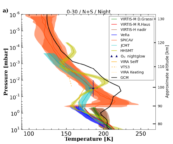
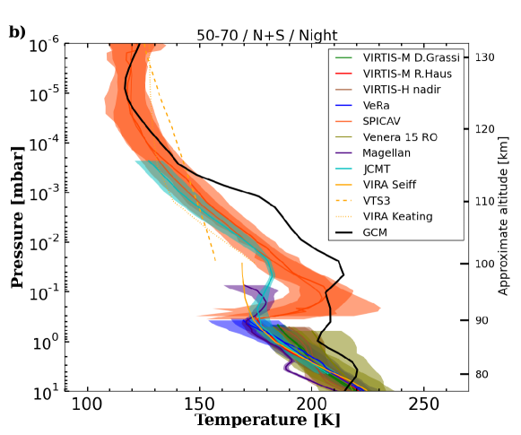
Figure 3: Compilation of available nighttime Venus temperature profiles above 80 km both from spacecrafts and ground based telescopes versus model predictions averaged at equatorial latitudes 0-30^∘ from Southern and Northern hemispheres (top panel) and 50^∘-70^∘ N/S (bottom panel). Corresponding approximate values for altitude is given on the right hand side of the panel. Panel a) and panel b) are adapted from Figure 15 and 17 in Limaye et al. [2017], respectively. See text for details. Uncertainties (one standard deviation) are either plotted as colored areas for averaged profiles in the same bin (Venus Express datasets, JCMT, HHSMT) or as error bars (O₂ nightglow). The IPSL-VGCM predicted profile is plotted with solid black line.

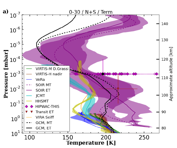
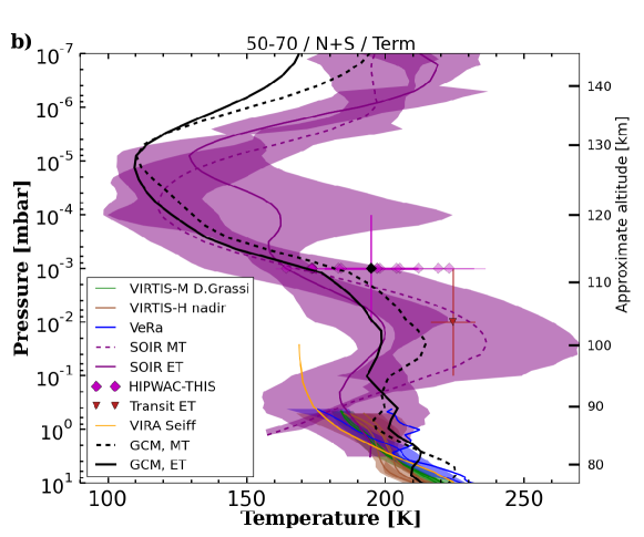
Figure 4: Same as Figure 3 but at the terminators (morning and evening) and with the addition of the mean temperature values retrieved at the evening terminator during the Venus transit in 2012. See text for details. Panel a) and panel b) are adapted from Figure 15 and 17 in Limaye et al. [2017], respectively. The IPSL-VGCM predicted profiles are in solid and dashed black lines for the ET and MT, respectively.

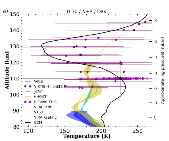
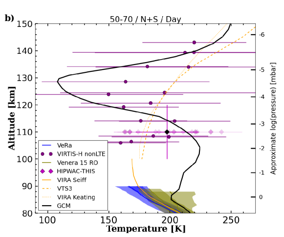
Figure 5: Same as Figure 3 but for daytime and with the addition of temperature retrieved from CO non-LTE emissions observed by VIRTIS/VEx. See text for details. Panel a) and panel b) are adapted from Figure 15 and 17 in Limaye et al. [2017], respectively.

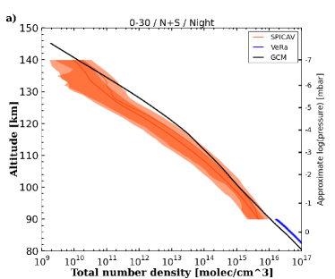
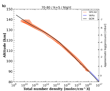
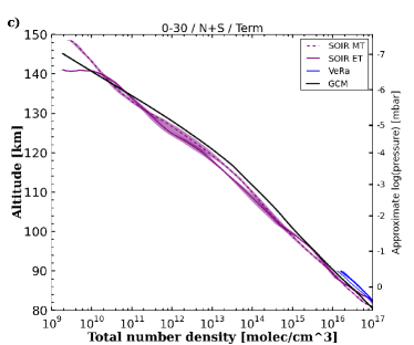
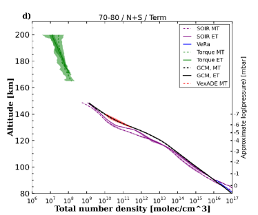
Figure 6: Measured total density profiles (molecule/cm³) retrieved with different Venus Express instruments at nighttime (Panels a and b) and at the terminators (Panels c and d) for two latitude bins 0-30^∘ and 70^∘-80^∘ (North/South averages) as indicated. The colored areas mark the uncertainty of the respective averaged profiles at one standard deviation. The figures are adapted from Figures 20 and 23 in Limaye et al. [2017]. Model predictions averaged at same latitudes and local time as observations are plotted with solid and dashed black lines. Vertical axis is given in altitudes, and approximate pressure (in mbar) is shown as the right hand side vertical axis.

Table 2: Observations of Temperature, CO₂, CO and O densities used in this paper (see Figures 3-6). Adapted from Table 1 in Limaye et al. [2017]

3.1 Temperature and total density

Our current knowledge of the Venus temperature structure comes from empirical models such as VIRA [Keating et al., 1985, Seiff et al., 1985] and VTS3 [Hedin et al., 1983], mostly based upon Pioneer Venus orbiter observations (PVO), and from many ground based and VEx observations [e.g. Clancy et al., 2008, 2012, Migliorini et al., 2012, Grassi et al., 2010, Mahieux et al., 2010, Gilli et al., 2015, Piccialli et al., 2015, Krause et al., 2018]. A comprehensive compilation of temperature retrievals since the publication of VIRA to Venus Express era was given in Limaye17, which provided for the first time a consistent picture of the temperature and density structure in the 40-180 km altitude range. This data intercomparison also aimed to make the first steps toward generating an updated VIRA model.

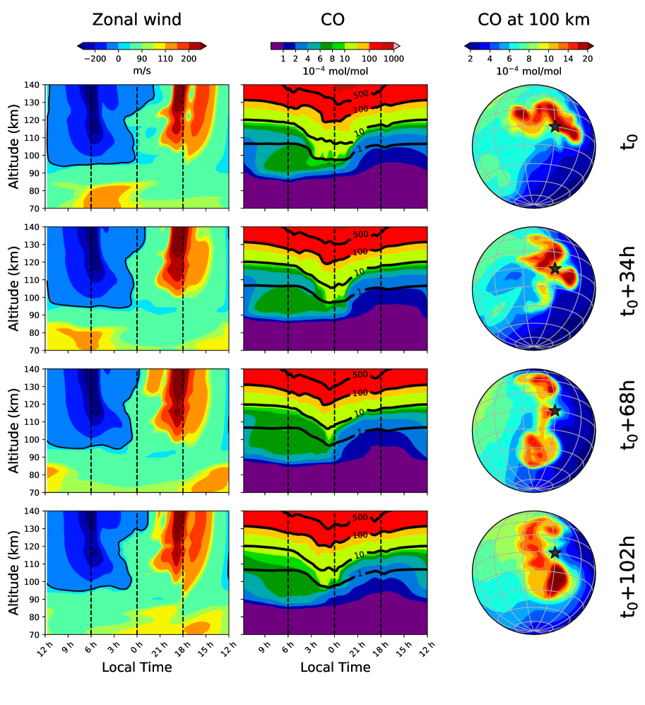
Figure 16: Four consecutive snapshots, from left to right, of: (1) 2D local time vs. altitude map of zonal wind averaged for latitudes 20^∘S-20^∘N, (2) 2D local time vs. altitude map of CO vmr [mol/mol] averaged for latitudes 20^∘S-20^∘N (3) 3D map of CO vmr [mol/mol] at 100 km, the AS point is indicated by a black star.

Beside the high variability observed even on short timescales, a succession of warm and cool layers above 80 km is one of remarkable feature that has been systematically detected. This was also correctly captured by model simulations [Gilli et al., 2017, Brecht and Bougher, 2012, Bougher et al., 2015] and interpreted as a combination of radiative and dynamical effects: the local maximum at daytime is produced by solar absorption in the non-LTE CO₂ IR bands, and then advected to the terminator, while a nighttime warm layer around 90 km is produced by subsidence of day-to-night air at the AS point. Above, the cold layer around 125-130 km is suggested to be caused by CO₂ 15 $\mu$m cooling. Nevertheless, especially above 100 km, temperature variation is large and the difference between individual experiments seems to be higher. Figures 3-5 are adapted from Figures 16-19 in Limaye17 and show a selection of observed temperature profiles together with IPSL-VGCM simulations on daytime (local time LT= 7h-17h), nighttime (LT= 19h-7h) and at the terminator regions (LT $\approx$ 18h and 6h), averaged in latitude bins. Here we show only equatorial region (0^∘-30^∘) and middle/high (50^∘-70^∘) latitudes, as examples. Figures 3 and 4 include retrieved temperature profiles from several instruments on board Venus Express binned in a similar latitude/local time range. Both channels of the Visible and Infrared Imaging Spectrometer (VIRTIS) are used here: VIRTIS-M temperature retrieved using CO₂ 4.3 $\mu$m band reported by [Grassi et al., 2014, Haus et al., 2015] and VIRTIS-H profiles as in Migliorini et al. [2012]. Data from solar and stellar occultation experiment on-board VEx, i.e. SOIR Piccialli et al. [2015] and SPICAV Mahieux et al. [2015], respectively, from Radio occultation measurements [Tellmann et al., 2009] and from O₂ nightglow observations at low latitudes [Piccioni and VIRTIS/Venus Express Team, 2009] are added. For daytime, only temperatures retrieved from non-LTE CO₂ emissions measured by VIRTIS/VEx [Gilli et al., 2015] are available above 110 km, as shown in Figure 5. Mean temperatures derived from the sunlight refraction in the mesosphere during the 2012 Venus transit [Tanga et al., 2012, Pere et al., 2016], and ground-based observations by the JCMT [Clancy et al., 2008, 2012], HHSTM [Rengel et al., 2008] and THIS/HIPWAC [Krause et al., 2018] are also taken into account. Empirical models such as VIRA [Seiff et al., 1985, Keating et al., 1985] and VTS3 [Hedin et al., 1983] are also plotted as reference.

As mentioned previously in Sec. 2.2, nightside temperatures (Fig. 3) predicted by the IPSL-VGCM are still overestimated in the 90-115 km altitude region, by 20 to 30 K, with a peak temperature altitude (around 100 km) that is in agreement with Earth-based observations (e.g. JCMT profiles), but about 5 km altitude higher than the peak of SPICAV temperature retrievals. Below 90 km, predicted temperatures tend to be at the upper limit of the range of observed values. At terminators (Fig. 4), simulated temperature profiles are in good agreement with most of the datasets, except for a cold bias of around 20 K above 130 km, compared to SOIR data. The current uncertainty in the collisional rate coefficients used in the non-LTE parameterization (see Section 2.1) is a possible candidate to explain this bias, since K_v-t variation has an impact on the temperature above 120 km approximately.

Dayside simulated temperature profiles (Fig. 5) reproduce the warm and cold layers observed near 110 km and 125 km, respectively, but tend to overestimate their amplitude. Note that the VIRA and VTS3 models, that were under-constrained in the 100-150 km altitude range, do not predict these temperature inversions. Nevertheless, it is difficult to get any conclusion from Figure 5, given the high error bars of daytime temperature measurements obtained with VIRTIS/VEx.

Retrieved vertical total density profiles from 80 km to 150 km are shown in Figure 6 as measured by the different Venus Express experiments mentioned above. In addition, density measurements from Venus Express Atmospheric Drag Experiment (VExADE) are included for high latitudes (panel d of Figure 6): between 130 and 140 km from accelerometer readings during aerobreaking [Müller-Wodarg et al., 2016], and in the altitude range 165-200 km from spacecraft torque measurements [Persson, 2015]. Nighttime densities are in very good agreement with SPICAV and VeRa, with the exception of the equatorial region, where IPSL-VGCM densities are a factor of 2-3 greater than SPICAV observations between 120 and 130 km. Densities retrieved by SOIR at the terminator are also up to a factor 2-3 lower then our simulations in the equatorial region, and up to 1 order of magnitude lower in the altitude between 100-140 km at high latitudes. However, in this region, it is worth noticing that our model predicted values fit very well with the VExADE density profile. The discrepancy with SOIR may be linked to the assumption of spherical homogeneous layers made by the authors and on the a-priori CO₂ mixing ratio. SOIR and SPICAV measured directly the CO₂ number density from its absorption structure, thus have to assume a CO₂ volume mixing ratio, taken from VTS3 semi-empirical model [Hedin et al., 1983] above 100 km. VTS3 is mainly based on PV measurements above 140 km and on model extrapolations assuming hydrostatic equilibrium between 100-140 km. This model revealed not to be adapted to represent the atomic oxygen densities derived from O₂ night-glow observations [Soret et al., 2012], the measured value being 3 times higher than predicted by VTS3. Moreover, the observed high variability of atmospheric quantities by VEx instruments was not reflected in previous empirical models (e.g. VIRA and VTS3) [Limaye et al., 2017]. Therefore, the uncertainties of SOIR profiles may reflect uncertainties in the VTS3 densities and have to be taken into account when comparing the observations with models.

3.2 CO densities

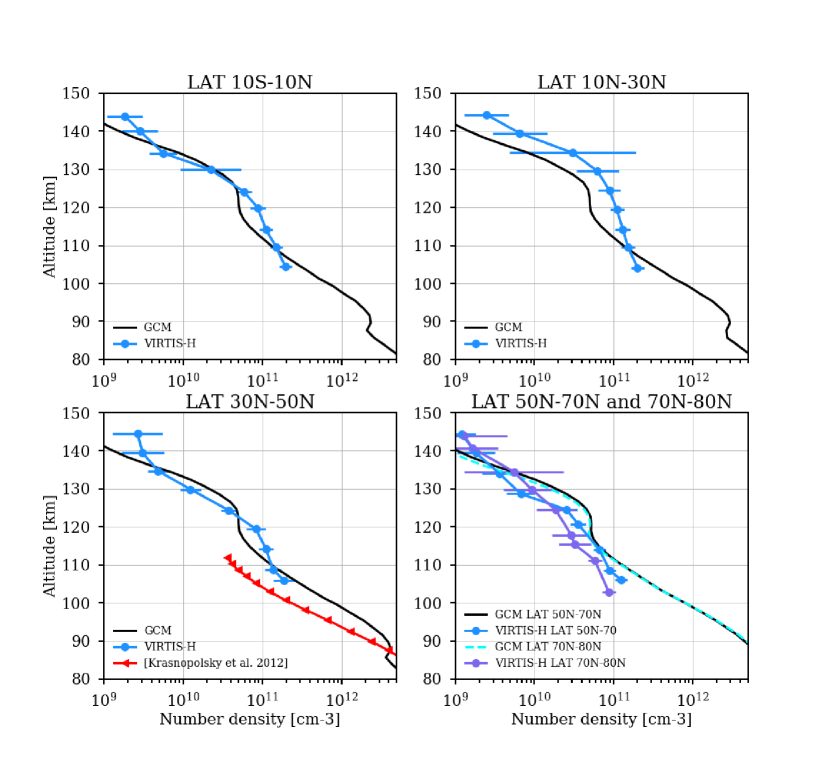
Figure 7: CO density retrieved by VIRTIS/VEx during daytime (LT 10h-14h) after Gilli et al. [2015] together with IPSL-VGCM averaged profiles binned at similar latitude and local time, as indicated in the panels. In addition, semi-empirical CO profile from Krasnopolsky [2012] representative of mean conditions is shown for comparison with mid-latitude (30^∘N-50^∘N) daytime averaged profiles.

Figures 7 to 10 show density of CO, compared with a selection of VEx experiments and ground-based measurements at different local time and latitudes. For daytime, retrieved CO density measurements are very scarce. We used here VIRTIS/VEx measurement in the altitude range 100-150 km as in Gilli et al. [2015] retrieved from non-LTE dayside IR CO emission at 4.7 $\mu$m. Below 112 km and for latitudes between 30^∘N-50^∘N, we also included the CO density profile from the semi-empirical model by Krasnopolsky [2012] which is representative of averaged values under intermediate solar conditions. We found that our results are very well comparable with observations in order of magnitude. However, daytime retrieved CO density between 110 and 125 km are about a factor 2 larger than our model profiles for most latitudes, except for high latitude bins (50^∘N-70^∘N) where instead observed CO densities are smaller than simulations, up to a factor 3. Those discrepancies could be related to the biases in the predicted temperature structure that we found above 90 km, the model being systematically warmer than the data between 90-110 km (approximately 10²—10^-1Pa), and colder between 120-150 km.

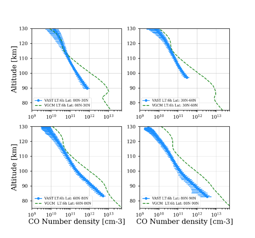
Figure 9: IPSL-VGCM simulated CO density profiles as function of altitude (green dashed lines) at the morning terminator (MT) (LT 6h) averaged at four selected latitude bins as indicated in the panels: 0^∘-30^∘N, 30^∘N-40^∘N, 60^∘N-80^∘N, 80^∘N-90^∘N. CO density profiles and relative error bars retrieved by SOIR/VEx at the MT in the same latitude bins are plotted in blue. VAST stands for: “Venus Atmosphere from SOIR data at the Terminator”, after Vandaele et al. [2016].

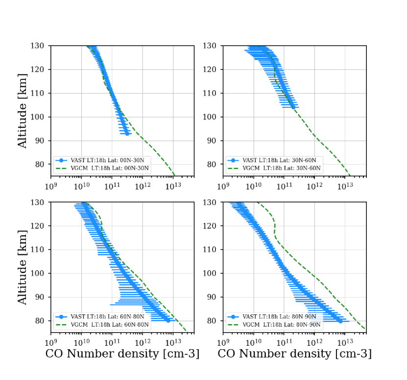
Figure 10: Same as Figure 9 but for evening terminator (ET), LT = 18h

Regarding the terminators (Figs. 9-10), our predicted CO densities are in overall agreement with SOIR dataset [Vandaele et al., 2016] in particular at evening terminator, but with larger differences with observed values below about 110 km on the morning side. The discrepancies are up to one order of magnitude between 90 and 100 km, and factor 2-3 elsewhere. Larger discrepancies are seen in the polar region (80^∘N-90^∘N), where our model is up to one order of magnitude larger than data for both MT and ET.

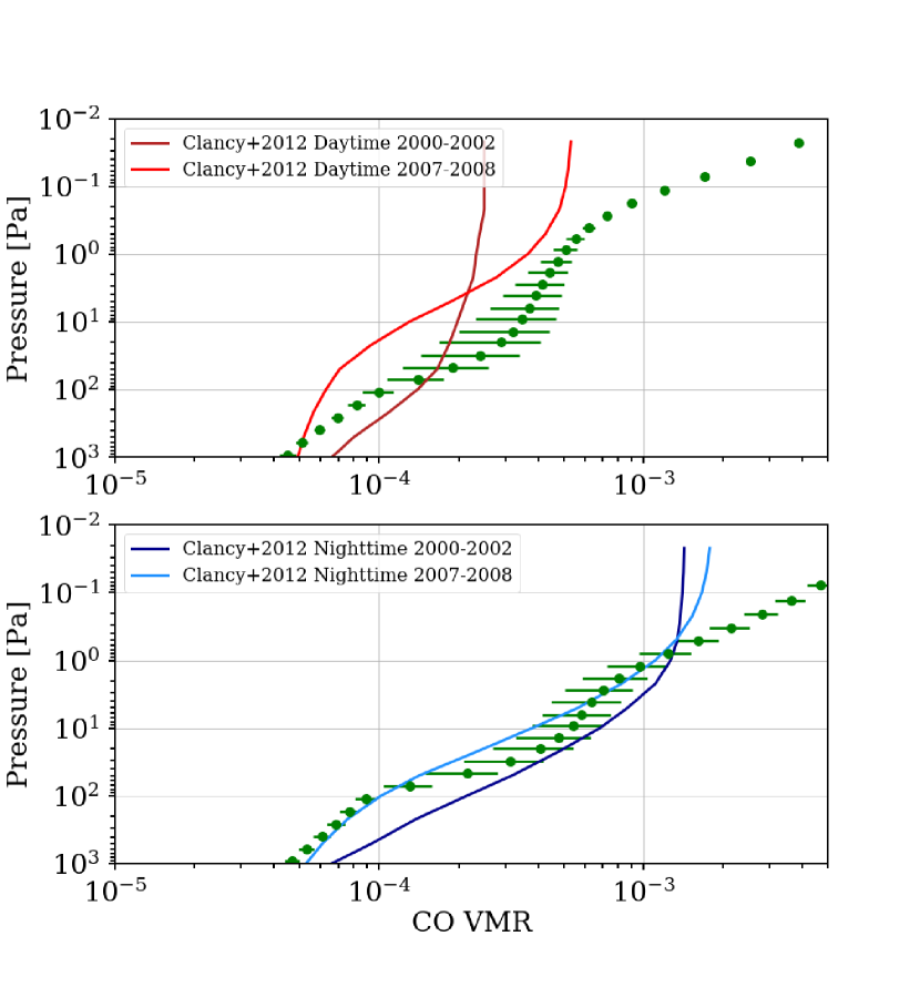
Figure 8: IPSL-VGCM CO volume mixing ratio profiles (green dots) as function of pressure, averaged in latitude bin 60^∘N-60^∘S, 10h-14h LT for daytime and 22h-2h for nighttime, with variability indicated as standard deviation of the average. CO profiles retrieved from sub-mm CO absorption line observations as in Clancy et al. [2012] for daytime (top panel) and nighttime (bottom panel) are also plotted. 2000-2002 disk average daytime/nighttime measurements are in dark red/blue solid lines, while 2007-2008 disk average daytime/nighttime measurements are in red/blue solid line.

Daytime and nighttime disk averaged CO measurements were also obtained in several ground-based campaigns [de Bergh et al., 1988, Clancy and Muhleman, 1991, Lellouch et al., 1989, Clancy et al., 2008, 2012] suggesting not only large variability over daily to weekly timescales, but also a distinct dayside versus nightside circulation in terms of zonal wind in particular [Clancy et al., 2012]. Figure 8 shows the comparison of model outputs and CO volume mixing ratio measurements during ground-based campaigns described in Clancy et al. [2012]. They represent 2001-2009 inferior conjunction sub-mm CO line observations, covering most of the disk (e.g. 60^∘S-60^∘N latitudes). Daytime model outputs are averaged for LT 10h-14h, and nighttime for LT 2h-22h, in the observed latitudinal bin. Our results are in general good agreement with observations for pressure ranges 10³-10 Pa, but above that pressure the trends are diverging (i.e. increasing volume mixing ratio (vmr) predicted by the model versus almost constant CO values suggested by observations). Nighttime measurements of the 2007-2008 campaign are within model dispersion bars (calculated as the standard deviation in the selected latitude/local time bin), and show a better agreement than 2000-2002 campaigns. Part of the difference between the two campaigns is likely related to the much reduced beam coverage for those early observations (Clancy, private communication).

Given the high variability of CO measurements over short time scales, it is difficult to find a general consensus among observations, and a clear defined trend. Our simulations indicate that the predicted abundances are affected by both the asymmetry of the SS-AS zonal flow at the terminator produced by non-orographic GW propagation in the lower thermosphere and the variability of zonal winds induced by Kelvin waves generated in the cloud deck, and propagating up to the mesosphere, as discussed in Navarro21. A possible interpretation of CO distribution is also provided in Section 5.

3.3 O densities

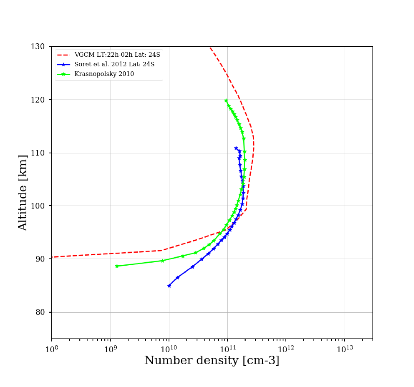
Figure 11: Nigthtime O density retrieved by VIRTIS/VEx from O₂ nightglow observations at the equator (Lat: 24^∘S) as in Soret et al. [2012] (blue line) and from Krasnopolsky [2012] semi-empirical model (green line). IPSL-VGCM simulated nighttime profile (LT: 22h-2h) for the same latitude is shown with red dashed line.

Only nighttime oxygen density measurements are available in the UMLT of Venus and they are derived from O₂ nightglow in the altitude range 85-110 km observed with VIRTIS/VEX, as described in Soret et al. [2012]. Figure 11 shows IPSL-VGCM results together with the observed profile near the equator (24^∘S) and nighttime O density extracted from a semi-empirical model by Krasnopolsky [2012]. In very good agreement with Soret et al. [2012], modeled values peak at 2$\times$10¹¹ cm^-3 around 110 km. Brecht et al. [2011] also found a similar value at midnight in their thermospheric GCM simulations at lower altitudes (3.4$\times$10¹¹ cm^-3 at 104 km). Below 95 km, O densities predicted by our model are decreasing much faster with altitude than observed in Soret et al. [2014], but this is still consistent with Krasnopolsky [2012]. A more complete description of the latitudinal and diurnal distribution of O predicted by the IPSL-VGCM is presented in the next section.

4 Diurnal and latitudinal variations of CO and O above 80 km by the IPSL-VGCM

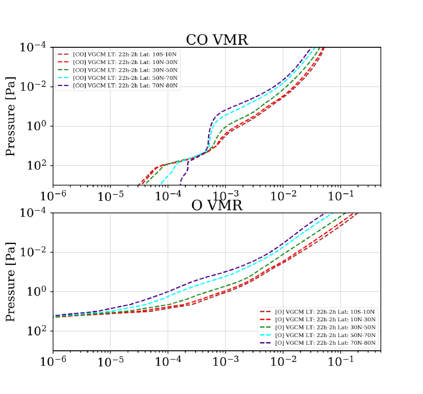
Figure 13: Latitudinal variations of CO and O vmr during nighttime predicted by the IPSL-VGCM. The latitude bins are indicated in each panel.

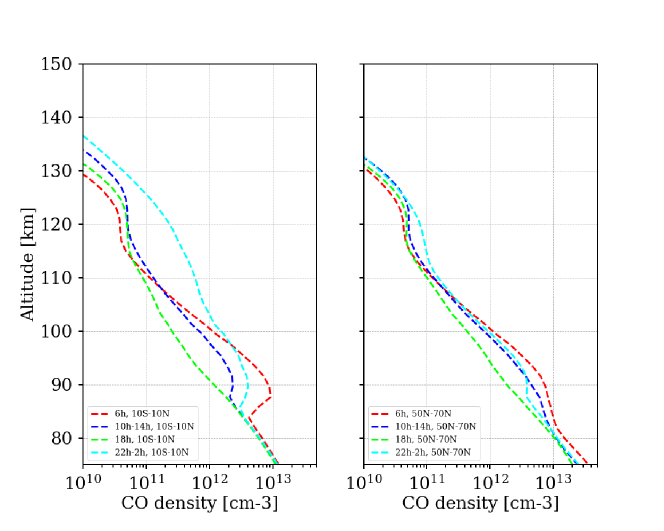
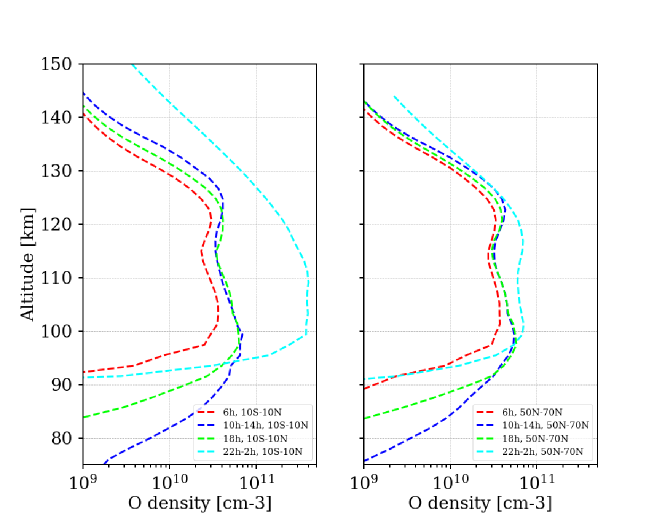
Figure 14: Local time variations of IPSL-VGCM CO (top panels) and O (bottom panels) density profiles at equatorial regions 10S-10N (left panels) and middle-high latitudes 50N-70N (right panels). Daytime and nighttime profiles are averaged between LT=10h-14h and LT=22h-2h, respectively. Evening (18h) and morning (6h) terminators are also plotted.

The latitudinal and diurnal variations of CO and O predicted by the IPSL-VGCM are analysed here in greater detail. Atomic oxygen chemical lifetime is shorter than carbon monoxide. Therefore the O mixing ratio decreases more rapidly with increasing pressure than CO, and its latitudinal variations are not significant in the GCM above $\sim$10 Pa (95 km approximately). This is clearly shown in Figures 12-13: CO and O vmr profiles by IPSL-VGCM as function of pressure are plotted for several latitude bins, at daytime (LT: 10h-14h) and nighttime (LT: 22h-2h).
In the lower mesosphere CO variations are primarily dominated by the global meridional dynamics, with CO vmr increasing from equator-to-pole [Tsang et al., 2008, Marcq et al., 2008]. At high latitudes, downward fluxes from the Hadley-type cell circulation bring air enriched in CO, whereas the ascending branch of these cells has the opposite effect near the equator [Marcq et al., 2008]. This equator-to-pole variation is predicted by our model below 1 Pa ($\sim$ 97-100 km), while oxygen vmr variation is negligible. In the upper mesosphere (above 1 Pa), CO as other light species is expected to pile up at the converging stagnation point of the wind field (i.e. where the horizontal velocity converges to zero). This point can be displaced from the anti-solar point when the circulation is not simply the SS-AS flow. Our simulations show that the CO nighttime bulge is shifted toward the morning between 85 and 100 km approximately, notably around the equator (see Figure 14), suggesting that CO is preferentially transported westwards in the transition region. Interestingly, Lellouch et al. [2008] observations showed a moderate (factor 2) CO enhancement near the morning terminator, although there are no systematic observations supporting this enhancement of CO on the morning side.

O chemical lifetime is shorter than the characteristic times of the atmospheric dynamics below 1 Pa approximately, where changes in vmr are driven by chemistry. The opposite is expected above 100 km, where the dynamical effects dominate [Brecht et al., 2011]. The atomic oxygen density peaks at midnight at the equator between 100 and 110 km, and it is about 1 order of magnitude larger than density values at the same altitude, at noon. The daytime peak is also located below 100 km. This enhancement from day to night side was also predicted in the Venus GCM by Brecht et al. [2011](e.g. a factor of 6 larger), and it is the result of efficient transport of atomic oxygen atoms from their day sources to their nightside chemical loss at and below about 110 km. In addition, our model predicts a second peak around 120 km (Figure 14), clearly defined for local time 10h-14h and at terminator, but weaker at midnight. Unfortunately, no observational data can be used to validate those trends for daytime and terminator. Only O density retrieved indirectly from O₂ nightlow are available so far, and they are in very good agreement with our prediction (see Figure 11). The origin of this second peak is beyond the scope of this paper and deserves a dedicated theoretical study, supported by systematic measurements of O densities.

5 Discussion: dynamical implications

5.1 Impact of the Kelvin wave

Several studies [Hueso et al., 2008, Clancy et al., 2012, Gérard et al., 2014, Lellouch et al., 2008, Moullet et al., 2012] indicated that both retrograde zonal and SS-AS flows affect the global distribution of CO, O and other light species at mesospheric altitudes (70-120 km). Those chemical tracers are transported by winds and are expected to pile up at the converging stagnation point of the wind. This point is usually at midnight (LT=0h) for pure SS-AS flow but it can be displaced toward the morning terminator if westward retrograde zonal flow is added. The position of the maximum and its magnitude depend on the relative values of equatorial velocity and a maximum cross-terminator velocity. The majority of Doppler winds retrieved at mesospheric and lower thermospheric altitudes [Clancy et al., 2008, 2012, Rengel et al., 2008, Widemann et al., 2007, Gurwell et al., 1995] suggested local time variation of the wind velocity and the presence of a substantial retrograde zonal flow at altitudes above 90 km. Lellouch et al. [2008] observations showed a moderate (factor of 2) CO enhancement near the morning terminator, and Gurwell et al. [1995] showed a CO maximum centered at 3h30 at 95 km, and at 2h at 100 km, approaching 2$\times$10^-3 volume mixing ratio.

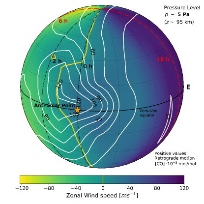
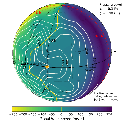
Figure 15: 3D maps of Venus nightside at 5 Pa (left) and 0.1 Pa (right) averaged for one Venus solar day, the anti-solar point is indicated with a star. Contour white lines: CO vmr and colors are zonal wind fields. Yellow lines indicate where the horizontal wind converges to zero values. The location of the terminator is represented by red dashed lines.

This retrograde imbalance of the flow towards the morning side is also predicted by our model. CO nighttime bulge is not located at the AS-point but shifted toward the morning (see Figure 15 and Figure 16) and in very good agreement with Gurwell et al. [1995]. The companion paper Navarro21 describes how the nightside mesospheric circulation is perturbed by a Kelvin wave with a period of approximately 5 Earth days In our simulations the equatorial wave appears to be excited between the middle and upper cloud (60-65 km altitude) and it propagates downward as a Kelvin wave, faster than zonal wind but also upward. At the cloud top, this wave propagates slower than the mean zonal wind, while recent Akatsuki UV observations suggest that the Kelvin wave propagates faster [Imai et al., 2019]. Kelvin waves with wavenumber-1 have also been predicted by other model experiments [e.g Yamamoto and Takahashi, 2006, Yamamoto, 2019, Sugimoto et al., 2014] but contrarily to our simulations they are slower near the cloud base ($\sim$ 50 km), with a period of 5-6 days. On average, this perturbation shifts the convergence of equatorial zonal wind between LT 0h and 3h, as shown with the Venus-day averaged view of Figures 15, or the instantaneous views of Figure 16. In the second column of Figure 16 we show how CO, with a longer chemical lifetime than the Kelvin wave period, accumulates preferentially towards the morning terminator, particularly at altitudes 90 to 110 km. On the contrary, atomic oxygen (not shown here), with a shorter life span, peaks near the AS point. To our knowledge, there is no such observation of CO matching this GCM result. Kelvin wave impact on the nightside also enhances the poleward meridional circulation. As a consequence, CO and O are also periodically transported to high latitudes likewise, as explained in Navarro2021 and shown in the third column of Figure 16. The poleward episodes create the high-latitude events of oxygen nightglow observed by VEx as high as 80^∘ [Soret et al., 2014]. However, our GCM simulations did not produce such events at latitudes higher than 60^∘, probably due to SS-AS too strong in the simulations. Therefore, we would expect that high-latitude nighttime CO is also underestimated in these simulations. Figures 9-10 instead show that the GCM largely overestimate SOIR measurements at the terminator in the latitude range 80^∘N-90^∘N. There are not CO nighttime measurements available at high-latitudes to contrast this result so far. Another remarkable characteristic of the Venus upper atmosphere emerging from the IPSL-VGCM results is the quiet daytime upper mesosphere (above 100 km) compared with highly variable nighttime, in agreement with observations.

5.2 Impact of non-orographic GW

Non-orographic GW breaking above 100 km also have a modest impact on the CO concentration. Previous theoretical studies (e.g. Hoshino et al. [2013] and Zalucha et al. [2013]) included a GW-drag parameterization in their model to investigate the effect of GW on the general circulation in the Venusian mesosphere and thermosphere. Hoshino et al. [2013] found the existence of weak wind layer at $\sim$125 km, not seen in previous simulations which used the Rayleigh friction scheme. Instead, Zalucha et al. [2013] suggested that gravity waves did not propagate above an altitude of nearly 115 km at the terminator because of total internal reflection.
The non-orographic GW paramerization and the baseline parameters chosen here are described in A.2. An analysis of the horizontal distribution of the wind velocity driven by GW is beyond the scope of this work, but the role of non-orographic GW forcing to the retrograde zonal flow in the transition region may be identified in our simulations. They show a clear asymmetry of the SS-AS zonal flow between the morning and the evening branches and at altitudes above 100 km (see Figure 16). As just explained in section 5.1, this asymmetry is caused by Kelvin wave impacting the mesosphere, but also by non-orographic GW. Indeed, these waves deposit momentum where they break, above 10^-1 Pa (110 km approximately), decelerating wind speed (e.g. causing acceleration of the SS-AS morning branch and deceleration of the SS-AS evening branch). The GW drag predicted by our model is stronger at the terminator, as in previous studies [e.g. Alexander et al., 1992, Hoshino et al., 2013, Zalucha et al., 2013], but has similar times values for the morning and evening terminator near the equator, as shown in Figure 17. The deceleration of the evening branch of the SS-AS flow is stronger between LT 16h and LT 18h, with a maximum of $\sim$ 0.02 m s^-2 at 3$\times$10^-1 Pa. The acceleration instead occurs over larger local time and altitude ranges, reaching the maximum around LT 5h-8h (e.g. 0.018 m s^-2). Therefore, the mean zonal forcing integrated over local times (not shown here) is positive on average. All in all, the cause of the westwards dominant nightside winds and CO bulge towards the morning terminator is twofold: a westwards propagating Kelvin wave impacting the mesosphere, up to 110 km, and a weaker westwards acceleration by GW in the lower thermosphere, above 110 km.

6 Conclusions

This paper presents a comprehensive data-model comparison of temperature, CO₂, CO and O abundances in the Venus upper atmosphere using the results of an improved high resolution ground-to-thermosphere (0-150 km) version of the IPSL-VGCM. For this validation exercise we selected a collection of data from VEx experiments and coordinated ground-based campaigns available so far following Limaye17.

• Improvements of the non-LTE parameterization previously implemented in the IPSL-VGCM and described in B allow to predict a thermal structure in better agreement with observations. Both the intensity and the altitude of warm layer around 100 km is closer to measurements. The peak of temperature around midday and midnight is reduced by 40 K and 20 K, respectively and it is located about 10 km lower than in Gilli17. The temperature inversion observed by SOIR [Vandaele et al., 2016] around 125 km, with a minimum of 125-130 K is also very well captured by our model. Despite significant improvements, a number of discrepancies still remain. Nighttime temperature are still overestimated in the 90-115 km altitude region, by 20 to 30 K, with a peak temperature altitude $\sim$ 5 km higher than SPICAV [Piccialli et al., 2015] retrieved profiles. Below 90 km, predicted temperatures tend to be at the upper limit of the range of observed values. A cold bias of 20 K to 50 K above 130 km is systematically found, compared to SOIR data. A candidate to explain this bias is the uncertainty in the collisional rate coefficients used in the non-LTE parameterization, that have an impact on the heating/cooling rate at thermosphere layers. Daytime simulated temperature profiles reproduce the warm and cold layers observed near 110 km and 125 km, respectively, but tend to overestimate their amplitude.

• CO₂ observed densities are also in overall agreement with IPSL-VGCM results, with the exception of the equatorial region, where predicted values are 2-3 times larger than SPICAV between 120 and 130 and than SOIR everywhere. Our model predicts very well density profiles measured during the VExADE aerobraking experiment [Persson, 2015]. The tion on the a-priori of CO₂ mixing ratio used to retrieve density and temperature in SOIR may partially explain the discrepancies that we found, in addition to the temperature cold bias found above 130 km at the terminator, mentioned above.

• Regarding the CO and O, model predictions are very well comparable with observations in order of magnitude and trend. Discrepancies found at daytime with VIRTIS data [Gilli et al., 2015] at low/middle latitudes between 110 and 125 km (the model slightly underestimates the CO density) could be linked to the biases in the predicted temperature, the model being systematically warmer than the data between 90-110 km and colder between 120-150 km. At the terminator, CO densities are in overall agreement with SOIR dataset, in particular at the ET, but with larger differences (up to one order of magnitude between 90 and 100 km and a factor 2-3 elsewhere) at the MT, especially at low latitudes. O densities are in very good agreement with nighttime indirect measurements from O₂ nightglow, peaking at 2$\times 10^{11}$ cm^-3 around 110 km, as observed.

• The latitudinal and diurnal variation of CO and O has also been investigated. We found that the CO nighttime bulge is shifted toward the morning between 85 and 100 km, approximately, suggesting that CO is preferentially transported westwards in the transition region. This feature is supported by ground-based observations of CO at nighttime [Gurwell et al., 1995, Lellouch et al., 2008, Moullet et al., 2012] which suggested the presence of a substantial westward retrograde zonal flow at altitudes above 90 km. Atomic oxygen density instead peaks at midnight in the equatorial region between 100 and 110 km, and they are about one order of magnitude larger than at noon, at the same altitude, as a result of efficient transport of atomic oxygen atoms from their day sources to their nighttime chemical loss at and below the peak.

• Our model includes a non-orographic GW parameterization following a stochastic approach as in Lott et al. [2012], Lott and Guez [2013]. Both westward and eastward GW generated above typical convective cells propagate upwards. In our simulations they break mostly above 10^-1 Pa (110 km altitude approximately) and accelerate/decelerate zonal wind by momentum deposition near the terminator. The mean zonal forcing is positive on average, contributing to retrograde imbalance of the flow in the lower thermosphere, above 110 km.
  However, given the lack of systematic observations of GW, which are necessary to constrain model parameters, our experience with different GCM configurations let us conclude that the total zonal wind (i.e. averaged for all local times) value is very sensitive to many GCM quirks, and can be either negative or positive. Therefore, it is not excluded that this weak acceleration in the lower thermosphere is linked to the sensitivity of the model to unconstrained parameters.

• The increased horizontal resolution used in this paper had a negligible impact on the heating/cooling rate above 90 km compared to the lower resolution version in Gilli17, therefore a small influence on the validation of the temperature and densities. However, the shock-like feature above 110 km which reduces horizontal wind speeds and increases the number of large-scale eddies, is obtained only in the high-resolution case (see Navarro21). Those eddies may be responsible of the high variation observed in O₂ nightglow and not explained by other models using a lower resolution in the thermosphere [Hoshino et al., 2013, Brecht et al., 2011].

• A retrograde imbalance of the flow towards the morning side is predicted by our model at equatorial regions, and interpreted as a combination of non-orographic GW asymmetric drag on the zonal wind and perturbation produced by a Kelvin wave generated at the cloud deck. The impact of this $\sim$5 Earth day wave on the middle/upper atmosphere of Venus is described in details in the companion paper Navarro21.

Figures

Figure 17: Local time-pressure distribution of the GW zonal drag (contours) integrated over all latitudes ($\theta$) and normalized by $\cos$($\theta$) to account for conservation of angular momentum. Zonal winds (color) at equator regions (10^∘S-10^∘N) are also shown. Solid line indicates acceleration, dotted line deceleration. Positive zonal wind values are westward and negative zonal wind values are eastward. Dashed-line indicates the region where the zonal wind converges to zero.

Appendix A Non-orographic GW parameterization

A.1 Formalism

The scheme implemented here is based on a stochastic approach, as fully described in Lott et al. [2012] and Lott and Guez [2013], also successfully implemented in the LMD Mars GCM [Gilli et al., 2020]. In such a scheme, a finite number of waves (here M = 8), with characteristics chosen randomly, are launched upwards at each physical time-step ($\delta t$ = 1.5 min) from every horizontal grid point to simulate their global effect. The question of the location of the non-orographic GW sources is a difficult one and given the lack of information on the location of GW sources, launching the gravity waves at each grid point, and at a fixed altitude, is probably the simplest assumption. The number of waves is given as M = NK $\times$ NO $\times$ NP, with NK = 2 values of GW horizontal wave-numbers, NO = 2 absolute values of phase speed, and NP = 2 directions (westward and eastward) of phase speed. This approach allows the model to treat a large number of waves at a given time $t$ by adding the effect of those M waves to that of the waves launched at previous steps, with a remnant time constant $\Delta t$ chosen to 1 Earth day (as for Earth and Mars).
The GW spectrum is then discretised in $\sim$ 7700 stochastic harmonics (M $\times\Delta t/\delta t$) which contribute to the wave field each day and at a given horizontal grid point. $\Delta t$ is a characteristic time interval which contains the GW life cycle (i.e. from its generation to wave break) and which has to exceed significantly the GCM time step $\delta t$. On Earth, GW theory indicates that atmospheric disturbances induced by convection have life cycles with duration $\Delta t$ around 1 day ($\Delta t$ = 24h)[Lott and Guez, 2013]. Here, as a first approximation we adopted this value ($\Delta t\gg\delta t=1.5$ min ). At each time $t$ the vertical velocity field $w^{\prime}$ of an upward propagating GW can be represented by the sum over harmonics:

$$w^{\prime}=\sum_{n=1}^{\infty}C_{n}w^{\prime}_{n}$$ (1)

where $C_{n}$ are normalization coefficients such that $\sum_{n=1}^{\infty}C_{n}^{2}=1$. It is assumed that each of the $w^{\prime}_{n}$ can be treated independently from the others, and each $C_{n}^{2}$ can be viewed as the probability that the wave field is represented by $w^{\prime}_{n}$ (see also the expression for $C_{n}$ in Equation 6). This formalism is then applied to a very simple multi-wave parameterization, in which $w^{\prime}_{n}$ represents a monochromatic wave as follows

$$w^{\prime}_{n}=\Re\left\{\hat{w}_{n}(z)e^{z/2H}e^{i(k_{n}x+l_{n}y-\omega_{n}t)}\right\}$$ (2)

where the wavenumbers $k_{n}$, $l_{n}$ and frequency $\omega_{n}$ are chosen randomly. In Equation 2, H$\sim$4 km is a middle atmosphere characteristic vertical scale for Venus [Lee et al., 2012, Mahieux et al., 2015] and z is the log-pressure altitude z = H $\ln$(P_r/P), with $P_{r}$ a reference pressure (P_r = $5\times 10^{4}$ Pa, taken here at the height of the source (i.e. above typical convective cells, $z\sim$ 55 km). To evaluate the amplitude $\hat{w}_{n}(z)$, it is randomly chosen at a given launching altitude $z_{0}$, and then iterated from one model level $z_{1}$ to the next $z_{2}$ by a Wentzel-Kramers-Brillouin (WKB) approximation (see Equation 4 of Lott et al. [2012] for details). Using that expression plus the polarization relation between the amplitudes of large scale horizontal wind $\hat{u}$ and vertical wind $\hat{w}$ (not shown here), we can deduce the Eliassen-Palm (EP) flux (vertical momentum flux of waves),

$$\vec{F}^{z}(k,l,\omega)=\Re\{\rho_{r}\vec{\hat{u}}\hat{w^{*}}\}=\rho_{r}\frac{\vec{k}}{|\vec{k}|^{2}}m(z)||\hat{w}(z)||^{2}$$ (3)

with $k,l$ the horizontal wavenumber and $\omega$ the frequency of the vertical velocity field. This last one is included in the WKB non-rotating approximation for the vertical wavenumber $m=\frac{N|\vec{k}|}{\Omega}$, with $\Omega=\omega-\vec{k}\vec{u}$ and N the Brunt-Vaisala frequency (see Lott et al. [2012] for details). In Equation (3), $\rho_{r}$ is the density at the reference pressure level $P_{r}$.
In this scheme, both $\hat{w}_{n}$ and the EP-flux at a given launching altitude $z_{0}$ (see Section A.2) are randomly chosen. To move from one model level to the next model level above, the EP-flux is essentially conserved, but a small diffusivity is allowed, $\nu=\mu/\rho_{0}$, which can be included by replacing $\Omega$ with $\Omega+i\nu m^{2}$. This small diffusivity is here to guarantee that the waves are ultimately dissipated over the few last model levels, if they have not been before (hence the division by the density $\rho_{0}$). In addition, this new EP-flux amplitude is limited to that produced by a saturated monochromatic wave $\hat{w}_{s}$ following Lindzen [1981]:

$$\hat{w}_{s}=S_{c}\frac{\Omega^{2}}{|\vec{k}|N}e^{-z/2H}\frac{k^{*}}{|\vec{k}|}$$ (4)

or either $\hat{w}$ = 0 when $\Omega$ changes sign, to treat critical levels. In Equation 4, $S_{c}$ is a tunable parameter and $k^{*}$ a characteristic horizontal wavelength corresponding to the longest wave being parameterized (see more details in Sec. A.2)
Finally, the accelerations $\rho^{-1}\delta_{z}\vec{F}^{z}_{n^{\prime}}$ ($n^{\prime}$= 1, M) produced by the GW drag on the winds are computed. Since $w^{\prime}_{n}$s are independent realizations, the mean acceleration they produce is the average of these M acceleration. Thus, the averaged acceleration is first redistributed over the longer time scale $\Delta t$ by re-scaling it by $\delta t$/$\Delta t$ and second, the auto-regressive (AR-1) relation described in [Lott et al., 2012] is used as follows:

$$\left(\frac{\delta\vec{u}}{\delta t}\right)_{GWs}^{t}=\frac{\delta t}{\Delta t}\frac{1}{M}\sum_{n^{\prime}=1}^{M}\frac{1}{\rho_{0}}\frac{\delta\vec{F}^{z}_{n^{\prime}}}{\delta z}+\frac{\Delta t-\delta t}{\Delta t}\left(\frac{\delta\vec{u}}{\delta t}\right)_{GWs}^{t-\delta t}$$ (5)

This indicates that, at each time step, M new waves are promoted by giving them the largest probability to represent the GW field, and the probabilities of all the others are degraded by the multiplicative factor $(\Delta t-\delta t)/\Delta t$. As explained in Lott et al. [2012], by expressing the cumulative sum underneath the AR-1 relation in Equation 5, the formalism for infinite superposition of stochastic waves is recovered by taking:

$$C^{2}_{n}=\left(\frac{\Delta t-\delta t}{\Delta t}\right)^{p}\frac{\delta t}{M\Delta t}$$ (6)

where $p$ is the nearest integer that rounds $(n-1)/M$ (i.e. toward lower values).

A.2 GW parameters setup

Here we describe the main tunable parameters used in the non-orographic GW scheme implemented in the IPSL-VGCM. The characteristics of every wave launched in the GCM are selected randomly with a prescribed box-shaped probability distribution, whose boundaries are key model parameters. These are chosen on the basis of observational constraints (whenever available) and theoretical considerations: each parameter has a physical meaning, as described below.

Source height and duration

First, considering that non-orographic GW are expected to be generated by deep cloud convective layer on Venus, and mostly driven by longwave radiation, we assumed that the non-orographic GW source is placed above typical convective cells (i.e. at $5.\times 10^{4}$ Pa, around 55 km of altitude), turned on all day, uniform and without latitudinal variation.

EP-flux amplitude

$F^{z}$ from Equation 3 gives the vertical rate of transfer of wave horizontal momentum per units of area. This value has never been measured in the Venus atmosphere and it represents an important degree of freedom in the parameterization of gravity waves. Thus, in our scheme we impose the maximum value of the probability distribution $F^{z}_{max}$ at the launching altitude z₀ (see previous point), at the beginning of the first run. In order to define $F^{0}_{max}$ we have explored typical values used in the literature to evaluate the order of magnitude of the EP-flux within the realm of what is realistic. It should be stressed here that the stochastic approach implemented in our scheme has the advantage of allowing to treat a wide diversity of emitted gravity waves, thereby a wide diversity of momentum fluxes. Our only setting is the maximum EP-flux amplitude at the launching altitude, that was fixed as 0.005 [kg m^-1 s^-2] (i.e. 5 mPa), following [Lefèvre et al., 2018] who simulated the gravity waves generated by the convective layer in a Large-Eddy-Simulation model describing realistically the Venusian convective activity.

Horizontal wavenumber

In our scheme the horizontal wave number amplitude is defined as in Lott et al. [2012] $k*<|k|<k_{s}$. The minimum value is $k*=1/\sqrt{\Delta{x}\Delta{y}}$, where $\Delta x$ and $\Delta y$ are comparable with the GCM horizontal grid. The maximum (saturated) value is $k_{s}<N^{2}/u$, $N$ being the Brunt-Vaisala frequency associated to the mean flow, and $u_{0}$ the mean zonal wind at the launching altitude. We kept the minimum and maximum values for the GW horizontal wavelength ($\lambda_{h}$ = $2\pi/k$ ) 50 km and 500 km, respectively as in Gilli17. Those values are within the observed range of GW wavelengths [Peralta et al., 2008, Piccialli et al., 2010, Tellmann et al., 2009, Altieri et al., 2014, Garcia et al., 2009] However, in order to correctly implement this parameterization with the increased resolution ($\delta$x and $\delta$y at the equator $\approx$ 400 km and 200 km in this study), we adapted the minimal horizontal wavenumber $k_{min}$ of individual waves as it follows:

$$k^{*}_{min}=max(k_{min},\frac{\pi}{A})$$ (7)

with $A$ the surface area of the grid cell. This value corresponds to the longest waves that one parameterizes with the current GCM horizontal resolution, larger wavelengths are explicitly resolved by the GCM.

Phase speed

Another key parameter is the amplitude of absolute phase speed $|c|=|\omega/k|$. As for the other tunable parameters, we impose the minimum $c_{min}$ and maximum $c_{max}$ values of the probability distribution at the beginning of the runs, and the model chooses randomly $|c|$ between $c_{min}$ and $c_{max}$. Here $c_{min}$ is set to 1 m/s (i.e for non-stationary GW) and $c_{max}$ is of the order of the zonal wind speed at the launching altitude ($u\approx 60~{}m/s$). Both eastward (c $>$ 0) and westward (c $<$ 0) moving GWs are considered.

Saturation parameter

$S_{c}$ is a tunable parameter in our scheme, on the right hand side of Equation 4, which controls the breaking of the GW by limiting the amplitude $w_{s}$. In the baseline simulation we set $S_{c}=1$.

Appendix B Improved Non-LTE parameterization set-up

The model includes 1-parameter formula that mimics the heating rates calculated by line-by-line non-LTE simulations for each pressure level $p$ and solar zenith angle $\mu$ (see Gilli17 for details). It is given by the following expression:

$$\frac{\partial T}{\partial t}(p,r,\mu)=\frac{\partial T}{\partial t}(p_{0},r_{0},0)\times\frac{r_{0}^{2}}{r^{2}}\sqrt{\frac{p_{0}}{p}\widetilde{\mu}}\Big{(}1+\frac{p_{1}}{p}\Big{)}^{-b}$$ (8)

where several orbital assumptions for Venus were considered: a circular planetary orbit with a mean solar distance of $r=r_{0}=$ 0.72 AU, no obliquity, and no seasonal variation. The cosine of the solar zenith angle $\widetilde{\mu}$ is corrected for atmospheric refraction using the following function: $\widetilde{\mu}=[(1224\mu^{2}+1)/1225]^{\frac{1}{2}}$.

In this paper, the values of four non-LTE parameters used in Gilli17 are reviewed and adjusted: (i) cloud top pressure level in [$Pa$], $p_{0}$; (ii) heating rate per Venusian day (Vd) in [$Kday^{-1}$], $\frac{\delta T}{\delta t}(p_{0},r_{0},0)$; (iii) pressure below which non-LTE effects become significant in [$Pa$], $p_{1}$; and (iv) central pressure for transition from LTE to non-LTE radiation tendencies in [$Pa$], $ptrans$.

First, we tuned the parameter $p_{1}$ to 0.1 [$Pa$] and $ptrans$ to 0.2 [$Pa$], which better represent the transition from LTE to non-LTE radiation. Second, following a literature review on the observed altitude of cloud tops [Ignatiev et al., 2009, Haus et al., 2015] the mean cloud top altitude is approximately located between 69 and 74 km. We tested several pressure levels, $p_{0}$, in this range of altitudes with corresponding solar heating rates from look-up tables in Crisp [1986]. The selected combination of those four parameters is listed in Table 1 together with those used in Gilli17, for comparison. Figure 18 shows the predicted net radiative rates in the two works, at different local time. The daytime heating/cooling peaking at 0.5 Pa (about 100 km) is reduced by almost a factor 2, while morning and evening terminator heating peaks around 0.1 Pa are about 3 times smaller, compared with Gilli17 simulations. Interestingly, nighttime radiative tendencies are affected by the changes of non-LTE parameter values mostly in the thermosphere, above 0.1 Pa (110 km approximately), suggesting that the region below is dominated by dynamical tendencies (e.g the adiabatic heating produces the local warm layer at nighttime), consistent with GCM results by Brecht and Bougher [2012].

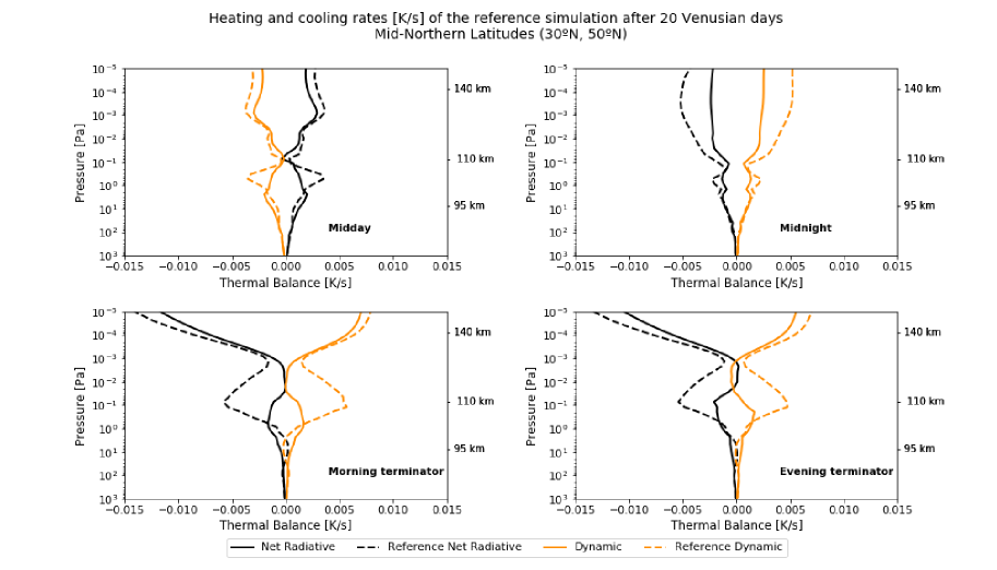
Figure 18: Net radiative and dynamical rates [K/s] obtained in this work for mid northern latitudes (30ºN-50ºN) after improving the Non-LTE parameterization for midday, nighttime and terminators, as indicated in the panels. For comparison, the rates obtained in a previous version of the IPSL-VGCM (Gilli17), labeled as “reference”, are also shown. Approximate altitudes are indicated on the right side of the panels.

Appendix C Bibliography styles

References

- Alexander et al. [1992] Alexander, M.J., Stewart, A.I.F., Bougher, S.W., 1992. Local-time asymmetries in the Venus thermosphere. LPI Contributions 789, 1–2.
- Altieri et al. [2014] Altieri, F., Migliorini, A., Zasova, L., Shakun, A., Piccioni, G., Bellucci, G., 2014. Modeling VIRTIS/VEX O2(a1#8710g) nightglow profiles affected by the propagation of gravity waves in the Venus upper mesosphere. Journal of Geophysical Research (Planets) 119, 2300–2316. doi:10.1002/2013JE004585.
- Ando et al. [2016] Ando, H., Sugimoto, N., Takagi, M., Kashimura, H., Imamura, T., Matsuda, Y., 2016. The puzzling Venusian polar atmospheric structure reproduced by a general circulation model. Nature Communications 7, 10398. doi:10.1038/ncomms10398.
- Bailey et al. [2008] Bailey, J., Meadows, V.S., Chamberlain, S., Crisp, D., 2008. The temperature of the Venus mesosphere from O2 (ag1) airglow observations. Icarus 197, 247–259. doi:10.1016/j.icarus.2008.04.007.
- Bougher et al. [2015] Bougher, S.W., Brecht, A.S., Schulte, R., Fischer, J., Parkinson, C.D., Mahieux, A., Wilquet, V., Vandaele, A., 2015. Upper atmosphere temperature structure at the Venusian terminators: A comparison of SOIR and VTGCM results. Planetary and Space Science 113, 336–346. doi:10.1016/j.pss.2015.01.012.
- Bougher et al. [1999] Bougher, S.W., Engel, S., Roble, R.G., Foster, B., 1999. Comparative terrestrial planet thermospheres 2. Solar cycle variation of global structure and winds at equinox. Journal of Geophysical Research 104, 16591–16611. doi:10.1029/1998JE001019.
- Bougher et al. [2006] Bougher, S.W., Rafkin, S., Drossart, P., 2006. Dynamics of the Venus upper atmosphere: Outstanding problems and new constraints expected from Venus Express. Planetary and Space Science 54, 1371–1380. doi:10.1016/j.pss.2006.04.023.
- Brecht and Bougher [2012] Brecht, A.S., Bougher, S.W., 2012. Dayside thermal structure of Venus’ upper atmosphere characterized by a global model. Journal of Geophysical Research (Planets) 117, 8002. doi:10.1029/2012JE004079.
- Brecht et al. [2011] Brecht, A.S., Bougher, S.W., Gérard, J.C., Parkinson, C.D., Rafkin, S., Foster, B., 2011. Understanding the variability of nightside temperatures, NO UV and O2 IR nightglow emissions in the Venus upper atmosphere. Journal of Geophysical Research (Planets) 116, 8004. doi:10.1029/2010JE003770.
- Clancy and Muhleman [1991] Clancy, R.T., Muhleman, D.O., 1991. Long-term (1979-1990) changes in the thermal, dynamical, and compositional structure of the Venus mesosphere as inferred from microwave spectral line observations of C-12O, C-13O, and CO-18. Icarus 89, 129–146. doi:10.1016/0019-1035(91)90093-9.
- Clancy et al. [2015] Clancy, R.T., Sandor, B.J., Hoge, J., 2015. Doppler winds mapped around the lower thermospheric terminator of Venus: 2012 solar transit observations from the James Clerk Maxwell Telescope. Icarus 254, 233–258. doi:10.1016/j.icarus.2015.03.031.
- Clancy et al. [2012] Clancy, R.T., Sandor, B.J., Moriarty-Schieven, G., 2012. Thermal structure and CO distribution for the Venus mesosphere/lower thermosphere: 2001-2009 inferior conjunction sub-millimeter CO absorption line observations. Icarus 217, 779–793. doi:10.1016/j.icarus.2011.05.032.
- Clancy et al. [2008] Clancy, R.T., Sandor, B.J., Moriarty-Schieven, G.H., 2008. Venus upper atmospheric CO, temperature, and winds across the afternoon/evening terminator from June 2007 JCMT sub-millimeter line observations. Planetary and Space Science 56, 1344–1354. doi:10.1016/j.pss.2008.05.007.
- Crisp [1986] Crisp, D., 1986. Radiative forcing of the Venus mesosphere. I - Solar fluxes and heating rates. Icarus 67, 484–514. doi:10.1016/0019-1035(86)90126-0.
- Crisp et al. [1996] Crisp, D., Meadows, V.S., Bézard, B., de Bergh, C., Maillard, J.P., Mills, F.P., 1996. Ground-based near-infrared observations of the Venus nightside: 1.27-m O2(ag) airglow from the upper atmosphere. Journal of Geophysical Research 101, 4577–4594. doi:10.1029/95JE03136.
- de Bergh et al. [1988] de Bergh, C., Crovisier, J., Lutz, B.L., Maillard, J.P., 1988. Detection of CO infrared emission lines in spectra of Venus, in: Bulletin of the American Astronomical Society, p. 831.
- de Bergh et al. [2006] de Bergh, C., Moroz, V.I., Taylor, F.W., Crisp, D., Bézard, B., Zasova, L.V., 2006. The composition of the atmosphere of Venus below 100 km altitude: An overview. Planetary and Space Science 54, 1389–1397. doi:10.1016/j.pss.2006.04.020.
- Drossart et al. [2007a] Drossart, P., Piccioni, G., Gérard, e.a., 2007a. A dynamic upper atmosphere of Venus as revealed by VIRTIS on Venus Express. Nature 450, 641–645. doi:10.1038/nature06140.
- Drossart et al. [2007b] Drossart, P., Piccioni, G., Lopez-Valverde, M.A., Gilli, G., Coradini, A., Bibring, J.P., VIRTIS/Venus Express Team, VIRTIS/Rosetta Team, OMEGA/Mars Express Team, 2007b. Carbon Dioxide Non-LTE Emission In The Telluric Upper Atmospheres, in: AAS/Division for Planetary Sciences Meeting Abstracts #39, p. 45.06.
- Fukuhara et al. [2017] Fukuhara, T., Taguchi, M., Imamura, T., Hayashitani, A., Yamada, T., Futaguchi, M., Kouyama, T., Sato, T.M., Takamura, M., Iwagami, N., Nakamura, M., Suzuki, M., Ueno, M., Hashimoto, G.L., Sato, M., Takagi, S., Yamazaki, A., Yamada, M., Murakami, S.y., Yamamoto, Y., Ogohara, K., Ando, H., Sugiyama, K.i., Kashimura, H., Ohtsuki, S., Ishii, N., Abe, T., Satoh, T., Hirose, C., Hirata, N., 2017. Absolute calibration of brightness temperature of the venus disk observed by the longwave infrared camera onboard akatsuki. Earth, Planets and Space 69, 141. URL: https://doi.org/10.1186/s40623-017-0727-y, doi:10.1186/s40623-017-0727-y.
- Garate-Lopez and Lebonnois [2018] Garate-Lopez, I., Lebonnois, S., 2018. Latitudinal variation of clouds’ structure responsible for Venus’ cold collar. Icarus 314, 1–11. doi:10.1016/j.icarus.2018.05.011.
- Garcia et al. [2009] Garcia, R.F., Drossart, P., Piccioni, G., López-Valverde, M., Occhipinti, G., 2009. Gravity waves in the upper atmosphere of Venus revealed by CO2 nonlocal thermodynamic equilibrium emissions. Journal of Geophysical Research (Planets) 114, E00B32. doi:10.1029/2008JE003073.
- Gérard et al. [2017] Gérard, J.C., Bougher, S.W., López-Valverde, M.A., Pätzold, M., Drossart, P., Piccioni, G., 2017. Aeronomy of the Venus Upper Atmosphere. Space Science Review 212, 1617–1683. doi:10.1007/s11214-017-0422-0.
- Gérard et al. [2014] Gérard, J.C., Soret, L., Piccioni, G., Drossart, P., 2014. Latitudinal structure of the Venus O2 infrared airglow: A signature of small-scale dynamical processes in the upper atmosphere. Icarus 236, 92–103. doi:10.1016/j.icarus.2014.03.028.
- Gilli et al. [2020] Gilli, G., Forget, F., Spiga, A., Navarro, T., Millour, E., Montabone, L., Kleinböhl, A., Kass, D.M., McCleese, D.J., Schofield, J.T., 2020. Impact of Gravity Waves on the Middle Atmosphere of Mars: A Non-Orographic Gravity Wave Parameterization Based on Global Climate Modeling and MCS Observations. Journal of Geophysical Research (Planets) 125, e05873. doi:10.1029/2018JE005873, arXiv:2002.00723.
- Gilli et al. [2017] Gilli, G., Lebonnois, S., González-Galindo, F., López-Valverde, M.A., Stolzenbach, A., Lefèvre, F., Chaufray, J.Y., Lott, F., 2017. Thermal structure of the upper atmosphere of Venus simulated by a ground-to-thermosphere GCM. Icarus 281, 55–72. doi:10.1016/j.icarus.2016.09.016.
- Gilli et al. [2015] Gilli, G., López-Valverde, M.A., Peralta, J., Bougher, S., Brecht, A., Drossart, P., Piccioni, G., 2015. Carbon monoxide and temperature in the upper atmosphere of Venus from VIRTIS/Venus Express non-LTE limb measurements. Icarus 248, 478–498. doi:10.1016/j.icarus.2014.10.047.
- Grassi et al. [2010] Grassi, D., Migliorini, A., Montabone, L., Lebonnois, S., Cardesìn-Moinelo, A., Piccioni, G., Drossart, P., Zasova, L.V., 2010. Thermal structure of Venusian nighttime mesosphere as observed by VIRTIS-Venus Express. Journal of Geophysical Research (Planets) 115, 9007. doi:10.1029/2009JE003553.
- Grassi et al. [2014] Grassi, D., Politi, R., Ignatiev, N.I., Plainaki, C., Lebonnois, S., Wolkenberg, P., Montabone, L., Migliorini, A., Piccioni, G., Drossart, P., 2014. The Venus nighttime atmosphere as observed by the VIRTIS-M instrument. Average fields from the complete infrared data set. Journal of Geophysical Research (Planets) 119, 837–849. doi:10.1002/2013JE004586.
- Gubenko et al. [2008] Gubenko, V.N., Andreev, V.E., Pavelyev, A.G., 2008. Detection of layering in the upper cloud layer of Venus northern polar atmosphere observed from radio occultation data. Journal of Geophysical Research (Planets) 113, E03001. doi:10.1029/2007JE002940.
- Gurwell et al. [1995] Gurwell, M.A., Muhleman, D.O., Shah, K.P., Berge, G.L., Rudy, D.J., Grossman, A.W., 1995. Observations of the CO bulge on Venus and implications for mesospheric winds. Icarus 115, 141–158. doi:Adddataforfield:Doidoi={10.1006/icar.1995.1085},.
- Haus et al. [2013] Haus, R., Kappel, D., Arnold, G., 2013. Self-consistent retrieval of temperature profiles and cloud structure in the northern hemisphere of Venus using VIRTIS/VEX and PMV/VENERA-15 radiation measurements. Planetary and Space Science 89, 77–101. doi:10.1016/j.pss.2013.09.020.
- Haus et al. [2015] Haus, R., Kappel, D., Arnold, G., 2015. Radiative heating and cooling in the middle and lower atmosphere of Venus and responses to atmospheric and spectroscopic parameter variations. Planetary and Space Science 117, 262–294. doi:10.1016/j.pss.2015.06.024.
- Hedin et al. [1983] Hedin, A.E., Niemann, H.B., Kasprzak, W.T., Seiff, A., 1983. Global empirical model of the Venus thermosphere. Journal of Geophysical Research 88, 73–83. doi:10.1029/JA088iA01p00073.
- Hoshino et al. [2013] Hoshino, N., Fujiwara, H., Takagi, M., Kasaba, Y., 2013. Effects of gravity waves on the day-night difference of the general circulation in the Venusian lower thermosphere. Journal of Geophysical Research (Planets) 118, 2004–2015. doi:10.1002/jgre.20154.
- Hueso et al. [2008] Hueso, R., Sánchez-Lavega, A., Piccioni, G., Drossart, P., Gérard, J.C., Khatuntsev, I., Zasova, L., Migliorini, A., 2008. Morphology and dynamics of Venus oxygen airglow from Venus Express/Visible and Infrared Thermal Imaging Spectrometer observations. Journal of Geophysical Research (Planets) 113, E00B02. doi:10.1029/2008JE003081.
- Ignatiev et al. [2009] Ignatiev, N.I., Titov, D.V., Piccioni, G., Drossart, P., Markiewicz, W.J., Cottini, V., Roatsch, T., Almeida, M., Manoel, N., 2009. Altimetry of the Venus cloud tops from the Venus Express observations. Journal of Geophysical Research (Planets) 114, 0. doi:10.1029/2008JE003320.
- Imai et al. [2019] Imai, M., Kouyama, T., Takahashi, Y., Yamazaki, A., Watanabe, S., Yamada, M., Imamura, T., Satoh, T., Nakamura, M., Murakami, S.y., et al., 2019. Planetary-scale variations in winds and uv brightness at the venusian cloud top: Periodicity and temporal evolution. Journal of Geophysical Research: Planets 124, 2635–2659.
- Irwin et al. [2008] Irwin, P.G.J., de Kok, R., Negrão, A., Tsang, C.C.C., Wilson, C.F., Drossart, P., Piccioni, G., Grassi, D., Taylor, F.W., 2008. Spatial variability of carbon monoxide in Venus’ mesosphere from Venus Express/Visible and Infrared Thermal Imaging Spectrometer measurements. Journal of Geophysical Research (Planets) 113, 0. doi:10.1029/2008JE003093.
- Jenkins et al. [1994] Jenkins, J.M., Steffes, P.G., Hinson, D.P., Twicken, J.D., Tyler, G.L., 1994. Radio Occultation Studies of the Venus Atmosphere with the Magellan Spacecraft. 2. Results from the October 1991 Experiments. Icarus 110, 79–94. doi:10.1006/icar.1994.1108.
- Keating et al. [1985] Keating, G.M., Bertaux, J.L., Bougher, S.W., Dickinson, R.E., Cravens, T.E., Hedin, A.E., 1985. Models of Venus neutral upper atmosphere - Structure and composition. Advances in Space Research 5, 117–171. doi:10.1016/0273-1177(85)90200-5.
- Kliore [1985] Kliore, A.J., 1985. Recent results on the Venus atmosphere from pioneer Venus radio occultations. Advances in Space Research 5, 41–49. doi:10.1016/0273-1177(85)90269-8.
- Krasnopolsky [2012] Krasnopolsky, V.A., 2012. A photochemical model for the Venus atmosphere at 47-112 km. Icarus 218, 230–246. doi:10.1016/j.icarus.2011.11.012.
- Krause et al. [2018] Krause, P., Sornig, M., Wischnewski, C., Kostiuk, T., Livengood, T.A., Herrmann, M., Sonnabend, G., Stangier, T., Wiegand, M., Pätzold, M., Mahieux, A., Vandaele, A.C., Piccialli, A., Montmessin, F., 2018. Long term evolution of temperature in the venus upper atmosphere at the evening and morning terminators. Icarus 299, 370–385. doi:10.1016/j.icarus.2017.07.030.
- Lebonnois et al. [2010] Lebonnois, S., Hourdin, F., Eymet, V., Crespin, A., Fournier, R., Forget, F., 2010. Superrotation of Venus’ atmosphere analyzed with a full general circulation model. Journal of Geophysical Research (Planets) 115, 6006. doi:10.1029/2009JE003458.
- Lebonnois et al. [2016] Lebonnois, S., Sugimoto, N., Gilli, G., 2016. Wave analysis in the atmosphere of Venus below 100-km altitude, simulated by the LMD Venus GCM. Icarus 278, 38–51. doi:10.1016/j.icarus.2016.06.004.
- Lee et al. [2012] Lee, Y.J., Titov, D.V., Tellmann, S., Piccialli, A., Ignatiev, N., Pätzold, M., Häusler, B., Piccioni, G., Drossart, P., 2012. Vertical structure of the Venus cloud top from the VeRa and VIRTIS observations onboard Venus Express. Icarus 217, 599–609. doi:10.1016/j.icarus.2011.07.001.
- Lefèvre et al. [2018] Lefèvre, M., Lebonnois, S., Spiga, A., 2018. Three-Dimensional Turbulence-Resolving Modeling of the Venusian Cloud Layer and Induced Gravity Waves: Inclusion of Complete Radiative Transfer and Wind Shear. Journal of Geophysical Research (Planets) 123, 2773–2789. doi:10.1029/2018JE005679.
- Lellouch et al. [1989] Lellouch, E., Gerin, M., Combes, F., Atreya, S., Encrenaz, T., 1989. Observations of the J = 1-0 CO lines in the Mars atmosphere - Radiodetection of C-13O and monitoring of C-12O. Icarus 77, 414–438.
- Lellouch et al. [2008] Lellouch, E., Paubert, G., Moreno, R., Moullet, A., 2008. Monitoring Venus’ mesospheric winds in support of Venus Express: IRAM 30-m and APEX observations. Planetary and Space Science 56, 1355–1367. doi:10.1016/j.pss.2008.06.010.
- Limaye et al. [2017] Limaye, S.S., Lebonnois, S., Mahieux, A., Pätzold, M., Bougher, S., Bruinsma, S., Chamberlain, S., Clancy, R.T., Gérard, J.C., Gilli, G., Grassi, D., Haus, R., Herrmann, M., Imamura, T., Kohler, E., Krause, P., Migliorini, A., Montmessin, F., Pere, C., Persson, M., Piccialli, A., Rengel, M., Rodin, A., Sandor, B., Sornig, M., Svedhem, H., Tellmann, S., Tanga, P., Vandaele, A.C., Widemann, T., Wilson, C.F., Müller-Wodarg, I., Zasova, L., 2017. The thermal structure of the venus atmosphere: Intercomparison of venus express and ground based observations of vertical temperature and density profiles. Icarus 294, 124 – 155. URL: http://www.sciencedirect.com/science/article/pii/S0019103516307138, doi:http://dx.doi.org/10.1016/j.icarus.2017.04.020.
- Lindzen [1981] Lindzen, R.S., 1981. Turbulence and stress owing to gravity wave and tidal breakdown. Journal of Geophysical Research 86, 9707–9714. doi:10.1029/JC086iC10p09707.
- Lott and Guez [2013] Lott, F., Guez, L., 2013. A stochastic parameterization of the gravity waves due to convection and its impact on the equatorial stratosphere. Journal of Geophysical Research (Atmospheres) 118, 8897–8909. doi:10.1002/jgrd.50705.
- Lott et al. [2012] Lott, F., Guez, L., Maury, P., 2012. A stochastic parameterization of non-orographic gravity waves: Formalism and impact on the equatorial stratosphere. Geophysical Research Letters 39, L06807. doi:10.1029/2012GL051001.
- Mahieux et al. [2015] Mahieux, A., Vandaele, A.C., Bougher, S.W., Drummond, R., Robert, S., Wilquet, V., Chamberlain, S., Piccialli, A., Montmessin, F., Tellmann, S., Pätzold, M., Häusler, B., Bertaux, J.L., 2015. Update of the Venus density and temperature profiles at high altitude measured by SOIR on board Venus Express. Planetary and Space Science 113, 309–320. doi:10.1016/j.pss.2015.02.002.
- Mahieux et al. [2010] Mahieux, A., Vandaele, A.C., Neefs, E., Robert, S., Wilquet, V., Drummond, R., Federova, A., Bertaux, J.L., 2010. Densities and temperatures in the Venus mesosphere and lower thermosphere retrieved from SOIR on board Venus Express: Retrieval technique. Journal of Geophysical Research (Planets) 115, 12014–+. doi:10.1029/2010JE003589.
- Mahieux et al. [2012] Mahieux, A., Vandaele, A.C., Robert, S., Wilquet, V., Drummond, R., Montmessin, F., Bertaux, J.L., 2012. Densities and temperatures in the Venus mesosphere and lower thermosphere retrieved from SOIR on board Venus Express: Carbon dioxide measurements at the Venus terminator. Journal of Geophysical Research (Planets) 117, 7001. doi:10.1029/2012JE004058.
- Marcq et al. [2008] Marcq, E., Bézard, B., Drossart, P., Piccioni, G., Reess, J.M., Henry, F., 2008. A latitudinal survey of CO, OCS, H2O, and SO2 in the lower atmosphere of Venus: Spectroscopic studies using VIRTIS-H. Journal of Geophysical Research (Planets) 113, E00B07. doi:10.1029/2008JE003074.
- Marcq et al. [2015] Marcq, E., Lellouch, E., Encrenaz, T., Widemann, T., Birlan, M., Bertaux, J.L., 2015. Search for horizontal and vertical variations of CO in the day and night side lower mesosphere of Venus from CSHELL/IRTF 4.53 m observations. Planetary and Space Science 113, 256–263. doi:10.1016/j.pss.2014.12.013.
- Mendonça and Read [2016] Mendonça, J.M., Read, P.L., 2016. Exploring the Venus global super-rotation using a comprehensive general circulation model. Planetary and Space Science 134, 1–18. doi:10.1016/j.pss.2016.09.001, arXiv:1609.06549.
- Migliorini et al. [2012] Migliorini, A., Grassi, D., Montabone, L., Lebonnois, S., Drossart, P., Piccioni, G., 2012. Investigation of air temperature on the nightside of Venus derived from VIRTIS-H on board Venus-Express. Icarus 217, 640–647. doi:10.1016/j.icarus.2011.07.013.
- Moullet et al. [2012] Moullet, A., Lellouch, E., Moreno, R., Gurwell, M., Sagawa, H., 2012. Wind mapping in Venus’ upper mesosphere with the IRAM-Plateau de Bure interferometer. Astronomy and Astrophysics 546, A102. doi:10.1051/0004-6361/201118451, arXiv:1202.5279.
- Müller-Wodarg et al. [2016] Müller-Wodarg, I.C.F., Bruinsma, S., Marty, J.C., Svedhem, H., 2016. In situ observations of waves in Venus’s polar lower thermosphere with Venus Express aerobraking. Nature Physics 12, 767–771. doi:10.1038/nphys3733.
- Navarro et al. [2021] Navarro, T., Gilli, G., Schubert, G., Lebonnois, S., Lefevre, F., Quirino, D., 2021. Venus’ upper atmosphere revealed by a gcm: I. structure and variability of the circulation. Icarus , 114400doi:https://doi.org/10.1016/j.icarus.2021.114400.
- Navarro et al. [2018] Navarro, T., Schubert, G., Lebonnois, S., 2018. Author Correction: Atmospheric mountain wave generation on Venus and its influence on the solid planet’s rotation rate. Nature Geoscience 11, 965–965. doi:10.1038/s41561-018-0257-7.
- Ohtsuki et al. [2008] Ohtsuki, S., Iwagami, N., Sagawa, H., Ueno, M., Kasaba, Y., Imamura, T., Yanagisawa, K., Nishihara, E., 2008. Distributions of the Venus 1.27-m O2 airglow and rotational temperature. Planetary and Space Science 56, 1391–1398. doi:10.1016/j.pss.2008.05.013.
- Peplowski et al. [2020] Peplowski, P.N., Lawrence, D.J., Wilson, J.T., 2020. Chemically distinct regions of Venus’s atmosphere revealed by measured N2 concentrations. Nature Astronomy 4, 947–950. doi:10.1038/s41550-020-1079-2, arXiv:1911.05598.
- Peralta et al. [2008] Peralta, J., Hueso, R., Sánchez-Lavega, A., Piccioni, G., Lanciano, O., Drossart, P., 2008. Characterization of mesoscale gravity waves in the upper and lower clouds of Venus from VEX-VIRTIS images. Journal of Geophysical Research (Planets) 113, E00B18. doi:10.1029/2008JE003185.
- Pere et al. [2016] Pere, C., Tanga, P., Widemann, T., Bendjoya, P., Mahieux, A., Wilquet, V., Vandaele, A.C., 2016. Multilayer modeling of the aureole photometry during the Venus transit: comparison between SDO/HMI and VEx/SOIR data. Astronomy and Astrophysics 595, A115. doi:10.1051/0004-6361/201628528, arXiv:1608.08544.
- Persson [2015] Persson, M., 2015. Venus thermosphere densities as revealed by Venus Express Torque and Accelerometer data. Master Thesis, Luleå Univ. of Technology.
- Piccialli et al. [2015] Piccialli, A., Montmessin, F., Belyaev, D., Mahieux, A., Fedorova, A., Marcq, E., Bertaux, J.L., Tellmann, S., Vandaele, A.C., Korablev, O., 2015. Thermal structure of Venus nightside upper atmosphere measured by stellar occultations with SPICAV/Venus Express. Planetary and Space Science 113, 321–335. doi:10.1016/j.pss.2014.12.009.
- Piccialli et al. [2010] Piccialli, A., Titov, D., Tellmann, S., Migliorini, A., Read, P., Grassi, D., Paetzold, M., Haeusler, B., Piccioni, G., Drossart, P., 2010. Thermal zonal winds in the Venus mesosphere from the Venus Express temperature soundings, in: 38th COSPAR Scientific Assembly, p. 1357.
- Piccialli et al. [2014] Piccialli, A., Titov, D.V., Sanchez-Lavega, A., Peralta, J., Shalygina, O., Markiewicz, W.J., Svedhem, H., 2014. High latitude gravity waves at the Venus cloud tops as observed by the Venus Monitoring Camera on board Venus Express. Icarus 227, 94–111. doi:10.1016/j.icarus.2013.09.012.
- Piccioni et al. [2007] Piccioni, G., Drossart, P., Sanchez-Lavega, A., Hueso, R., Taylor, F.W., Wilson, C.F., Grassi, D., Zasova, L., Moriconi, M., Adriani, A., Lebonnois, S., Coradini, A., Bézard, B., Angrilli, F., Arnold, G., Baines, K.H., Bellucci, G., Benkhoff, J., Bibring, J.P., Blanco, A., Blecka, M.I., Carlson, R.W., di Lellis, A., Encrenaz, T., Erard, S., Fonti, S., Formisano, V., Fouchet, T., Garcia, R., Haus, R., Helbert, J., Ignatiev, N.I., Irwin, P.G.J., Langevin, Y., Lopez-Valverde, M.A., Luz, D., Marinangeli, L., Orofino, V., Rodin, A.V., Roos-Serote, M.C., Saggin, B., Stam, D.M., Titov, D., Visconti, G., Zambelli, M., Ammannito, E., Barbis, A., Berlin, R., Bettanini, C., Boccaccini, A., Bonnello, G., Bouye, M., Capaccioni, F., Cardesin Moinelo, A., Carraro, F., Cherubini, G., Cosi, M., Dami, M., de Nino, M., Del Vento, D., di Giampietro, M., Donati, A., Dupuis, O., Espinasse, S., Fabbri, A., Fave, A., Veltroni, I.F., Filacchione, G., Garceran, K., Ghomchi, Y., Giustini, M., Gondet, B., Hello, Y., Henry, F., Hofer, S., Huntzinger, G., Kachlicki, J., Knoll, R., Driss, K., Mazzoni, A., Melchiorri, R., Mondello, G., Monti, F., Neumann, C., Nuccilli, F., Parisot, J., Pasqui, C., Perferi, S., Peter, G., Piacentino, A., Pompei, C., Reess, J.M., Rivet, J.P., Romano, A., Russ, N., Santoni, M., Scarpelli, A., Semery, A., Soufflot, A., Stefanovitch, D., Suetta, E., Tarchi, F., Tonetti, N., Tosi, F., Ulmer, B., 2007. South-polar features on Venus similar to those near the north pole. Nature 450, 637–640. doi:10.1038/nature06209.
- Piccioni and VIRTIS/Venus Express Team [2009] Piccioni, G., VIRTIS/Venus Express Team, 2009. The Visible and Infrared Thermal Imaging Spectrometer. in press ESA SP-1295. Eur. Space Agency Spec. Publ.. ESA Publications Division, Noordwijk, The Netherlands,.
- Rengel et al. [2008] Rengel, M., Hartogh, P., Jarchow, C., 2008. Mesospheric vertical thermal structure and winds on Venus from HHSMT CO spectral-line observations. Planetary and Space Science 56, 1368–1384. doi:10.1016/j.pss.2008.07.004, arXiv:0809.2743.
- Roldán et al. [2000] Roldán, C., López-Valverde, M.A., López-Puertas, M., Edwards, D.P., 2000. Non-LTE Infrared Emissions of CO2 in the Atmosphere of Venus. Icarus 147, 11–25. doi:doi={10.1006/icar.2000.6432},.
- Satoh et al. [2017] Satoh, T., Sato, T.M., Nakamura, M., Kasaba, Y., Ueno, M., Suzuki, M., Hashimoto, G.L., Horinouchi, T., Imamura, T., Yamazaki, A., Enomoto, T., Sakurai, Y., Takami, K., Sawai, K., Nakakushi, T., Abe, T., Ishii, N., Hirose, C., Hirata, N., Yamada, M., Murakami, S.y., Yamamoto, Y., Fukuhara, T., Ogohara, K., Ando, H., Sugiyama, K.i., Kashimura, H., Ohtsuki, S., 2017. Performance of Akatsuki/IR2 in Venus orbit: the first year. Earth, Planets, and Space 69, 154. doi:10.1186/s40623-017-0736-x.
- Schubert [1983] Schubert, G., 1983. General circulation and the dynamical state of the Venus atmosphere. pp. 681–765.
- Seiff et al. [1985] Seiff, A., Schofield, J.T., Kliore, A.J., Taylor, F.W., Limaye, S.S., 1985. Models of the structure of the atmosphere of Venus from the surface to 100 kilometers altitude. Advances in Space Research 5, 3–58. doi:10.1016/0273-1177(85)90197-8.
- Soret et al. [2012] Soret, L., Gérard, J.C., Montmessin, F., Piccioni, G., Drossart, P., Bertaux, J.L., 2012. Atomic oxygen on the Venus nightside: Global distribution deduced from airglow mapping. Icarus 217, 849–855. doi:10.1016/j.icarus.2011.03.034.
- Soret et al. [2014] Soret, L., Gérard, J.C., Piccioni, G., Drossart, P., 2014. Time variations of O2(a1) nightglow spots on the Venus nightside and dynamics of the upper mesosphere. Icarus 237, 306–314. doi:10.1016/j.icarus.2014.03.034.
- Sornig et al. [2008] Sornig, M., Livengood, T., Sonnabend, G., Kroetz, P., Stupar, D., Kostiuk, T., Schieder, R., 2008. Venus upper atmosphere winds from ground-based heterodyne spectroscopy of CO2 at 10m wavelength. Planetary and Space Science 56, 1399–1406. doi:10.1016/j.pss.2008.05.006.
- Stolzenbach [2016] Stolzenbach, A., 2016. Étude de la photochimie de Vénus à l’aide d’un modèle de circulation général. Ph.D. thesis.
- Sugimoto et al. [2014] Sugimoto, N., Takagi, M., Matsuda, Y., 2014. Waves in a Venus general circulation model. Geophysical Research Letter 41, 7461–7467. doi:10.1002/2014GL061807.
- Takagi and Matsuda [2007] Takagi, M., Matsuda, Y., 2007. Effects of thermal tides on the Venus atmospheric superrotation. Journal of Geophysical Research (Atmospheres) 112, D09112. doi:10.1029/2006JD007901.
- Tanga et al. [2012] Tanga, P., Widemann, T., Sicardy, B., Pasachoff, J.M., Arnaud, J., Comolli, L., Rondi, A., Rondi, S., Sütterlin, P., 2012. Sunlight refraction in the mesosphere of Venus during the transit on June 8th, 2004. Icarus 218, 207–219. doi:10.1016/j.icarus.2011.12.004, arXiv:1112.3136.
- Taylor and Grinspoon [2009] Taylor, F., Grinspoon, D., 2009. Climate evolution of Venus. Journal of Geophysical Research (Planets) 114, 0. doi:10.1029/2008JE003316.
- Taylor [1995] Taylor, F.W., 1995. Carbon monoxide in the deep atmospheres of Venus. Advances in Space Research 16, 81–. doi:10.1016/0273-1177(95)00253-B.
- Tellmann et al. [2009] Tellmann, S., Pätzold, M., Häusler, B., Bird, M.K., Tyler, G.L., 2009. Structure of the Venus neutral atmosphere as observed by the Radio Science experiment VeRa on Venus Express. Journal of Geophysical Research (Planets) 114, E00B36. doi:10.1029/2008JE003204.
- Tsang et al. [2008] Tsang, C.C.C., Irwin, P.G.J., Wilson, C.F., Taylor, F.W., Lee, C., de Kok, R., Drossart, P., Piccioni, G., Bezard, B., Calcutt, S., 2008. Tropospheric carbon monoxide concentrations and variability on Venus from Venus Express/VIRTIS-M observations. Journal of Geophysical Research (Planets) 113, E00B08. doi:10.1029/2008JE003089.
- Vandaele et al. [2016] Vandaele, A.C., Mahieux, A., Chamberlain, S., Ristic, B., Robert, S., Thomas, I.R., Trompet, L., Wilquet, V., Bertaux, J.L., 2016. Carbon monoxide observed in Venus’ atmosphere with SOIR/VEx. Icarus 272, 48–59. doi:10.1016/j.icarus.2016.02.025.
- von Zahn et al. [1983] von Zahn, U., Kumar, S., Niemann, H., Prinn, R., 1983. Composition of the venus atmosphere, in: Hunten, D.M., Colin, L., Donahue, T.M., Moroz, V.I. (Eds.), Venus. Univ. of Arizona Press, Tucson, AZ, pp. 299–430.
- Widemann et al. [2007] Widemann, T., Lellouch, E., Campargue, A., 2007. New wind measurements in Venus’ lower mesosphere from visible spectroscopy. Planetary and Space Science 55, 1741–1756. doi:10.1016/j.pss.2007.01.005.
- Yamamoto [2019] Yamamoto, M., 2019. Equatorial kelvin-like waves on slowly rotating and/or small-sized spheres: Application to venus and titan. Icarus 322, 103–113.
- Yamamoto et al. [2021] Yamamoto, M., Ikeda, K., Takahashi, M., 2021. Atmospheric response to high-resolution topographical and radiative forcings in a general circulation model of Venus: Time-mean structures of waves and variances. Icarus 355, 114154. doi:10.1016/j.icarus.2020.114154.
- Yamamoto and Takahashi [2006] Yamamoto, M., Takahashi, M., 2006. Superrotation Maintained by Meridional Circulation and Waves in a Venus-Like AGCM. Journal of Atmospheric Sciences 63, 3296–3314. doi:10.1175/JAS3859.1.
- Zalucha et al. [2013] Zalucha, A.M., Brecht, A.S., Rafkin, S., Bougher, S.W., Alexander, M.J., 2013. Incorporation of a gravity wave momentum deposition parameterization into the Venus Thermosphere General Circulation Model (VTGCM). Journal of Geophysical Research (Planets) 118, 147–160. doi:10.1029/2012JE004168.
- Zasova et al. [2006] Zasova, L.V., Moroz, V.I., Formisano, V., Ignatiev, N.I., Khatuntsev, I.V., 2006. Exploration of Venus with the Venera-15 IR Fourier spectrometer and the Venus Express planetary Fourier spectrometer. Cosmic Research 44, 349–363. doi:10.1134/S0010952506040083.