An Accelerated Method For Decentralized Distributed Stochastic Optimization Over Time-Varying Graphs

Abstract

We consider a distributed stochastic optimization problem that is solved by a decentralized network of agents with only local communication between neighboring agents. The goal of the whole system is to minimize a global objective function given as a sum of local objectives held by each agent. Each local objective is defined as an expectation of a convex smooth random function and the agent is allowed to sample stochastic gradients for this function. For this setting we propose the first accelerated (in the sense of Nesterov’s acceleration) method that simultaneously attains optimal up to a logarithmic factor communication and oracle complexity bounds for smooth strongly convex distributed stochastic optimization. We also consider the case when the communication graph is allowed to vary with time and obtain complexity bounds for our algorithm, which are the first upper complexity bounds for this setting in the literature.

I Introduction

Distributed algorithms have already about half a century history [1, 2, 3] with many applications including robotics, resource allocation, power system control, control of drone or satellite networks, distributed statistical inference and optimal transport, multiagent reinforcement learning [4, 5, 6, 7, 8, 9, 10, 11, 12]. Recently, development of such algorithms has become one of the main topics in optimization and machine learning motivated by large-scale learning problems with privacy constraints and other challenges such as data being produced or stored distributedly [13, 14, 15, 16, 17]. An important part of this research studies decentralized distributed optimization algorithms over arbitrary networks. In this setting a network of computing agents, e.g. sensors or computers, is represented by a connected graph in which two agents can communicate with each other if there is an edge between them. This imposes communication constraints and the goal of the whole system [18, 19, 20] is to cooperatively minimize a global objective using only local communications between agents, each of which has access only to a local piece of the global objective. Due to random nature of the optimized process or randomness and noise in the used data, a particular important setting is distributed stochastic optimization. Moreover, the topology of the network can vary in time, which may prevent fast convergence of an algorithm.

More precisely, we consider the following optimization problem

$$\min_{x\in\mathbb{R}^{d}}\left[f(x):=\frac{1}{n}\sum_{i=1}^{n}f_{i}(x)\right],\quad f_{i}(x):=\mathbb{E}_{\xi_{i}\sim{\mathcal{D}}_{i}}{\bf f}_{i}(x,\xi_{i}),$$ (1)

where $\xi_{i}$’s are random variables with probability distributions ${\mathcal{D}}_{i}$. For each $i=1,...,n$ we make the following assumptions: $f_{i}(x)$ is a convex function and that almost sure w.r.t. distribution ${\mathcal{D}}_{i}$, the function ${\bf f}_{i}(x,\xi_{i})$ has gradient $\nabla{\bf f}_{i}(x,\xi_{i})$, which is $L_{i}({\color[rgb]{0,0,0}\xi_{i}})$-Lipschitz continuous with respect to the Euclidean norm. Further, for each $i=1,...,n$, we assume that we know a constant $L_{i}\geqslant 0$ such that $\sqrt{\mathbb{E}_{{\color[rgb]{0,0,0}\xi_{i}}}L_{i}({\color[rgb]{0,0,0}\xi_{i}})^{2}}\leq L_{i}<+\infty$. Under these assumptions, $\mathbb{E}_{{\color[rgb]{0,0,0}\xi_{i}}}\nabla{\bf f}_{i}(x,\xi_{i})=\nabla f_{i}(x)$ and $f$ is $L_{i}$-smooth, i.e. has $L_{i}$-Lipschitz continuous gradient with respect to the Euclidean norm. Also, we assume that, for all $x$, and $i$

$$\mathbb{E}_{{\color[rgb]{0,0,0}\xi_{i}}}[\left\|\nabla{\bf f}_{i}(x,\xi_{i})-\nabla f_{i}(x)\right\|^{2}]\leqslant\sigma_{i}^{2},$$ (2)

where $\left\|\cdot\right\|$ is the Euclidean norm. Finally, we assume that each $f_{i}$ is $\mu_{i}$-strongly convex ($\mu_{i}>0$). Important characteristics of the objective in (1) are local strong convexity parameter $\displaystyle\mu_{l}=\min_{i}\mu_{i}$ and local smoothness constant $L_{l}=\max_{i}L_{i}$, which define local condition number $\kappa_{l}=L_{l}/\mu_{l}$, as well as their global counterparts $\mu_{g}=\frac{1}{n}\sum_{i=1}^{n}\mu_{i},\leavevmode\nobreak\ L_{g}=\frac{1}{n}\sum_{i=1}^{n}L_{i}$, $\kappa_{g}=L_{g}/\mu_{g}$. The global condition number may be significantly better than local (see e.g. [21] for details) and it is desired to develop algorithms with complexity depending on the global condition number. Moreover, we introduce a worst-case smoothness constant over stochastic realizations $\displaystyle L_{\xi}=\max_{i}\max_{\xi}L_{i}(\xi)$ and a maximum gradient norm at optimum $\displaystyle M_{\xi}=\max_{i}\max_{\xi}\left\|\nabla f_{i}(x^{*},\xi)\right\|$ and assume that these constants are well-defined (finite). Similarly to global smoothness and strong convexity constants, we introduce $\sigma_{g}^{2}=\frac{1}{n}\sum_{i=1}^{n}\sigma_{i}^{2}$.

To introduce the distributed optimization setup, we assume that communication constraints in the computational network are represented by an undirected communication graph which may vary with time. Namely, the network is modeled with a sequence of graphs $\left\{\mathcal{G}^{k}=(V,E^{k})\right\}_{k=0}^{\infty}$. We note that the set of vertices remains the same, while set of edges is allowed to change with time. Each agent in the network corresponds to a graph vertex and communication at time slot $k$ is possible only between nodes which are connected by an edge at this time slot. Further, each agent $i$ has access only to iid samples from ${\mathcal{D}}_{i}$ and corresponding stochastic gradients $\nabla{\bf f}_{i}(x,\xi_{i})$. The goal of the whole network is to solve the minimization problem (1) by using only communication between neighboring nodes. The performance of decentralized optimization algorithms depends on the characteristic number $\chi$ of the network that quantifies its connectivity and how fast the information is spread over the network. The precise definition will be given later.

I-A Related work

In centralized setting optimal methods exist [22] for the considered setting of smooth strongly convex stochastic optimization, as well as many algorithms for other settings [23, 24, 25, 26]. Decentralized distributed optimization introduces several challenges, one of them being that one has to care about two complexities: number of oracle calls which are made by each agent and the number of communication steps, which are sufficient to reach a given accuracy $\varepsilon$. In the simple case of all constants $\mu_{i},L_{i},\sigma_{i}$ being independent on $i$, the oracle complexity lower bound [21, 27] $\Omega\left(\max\left\{\frac{\sigma^{2}}{n\mu\varepsilon},\sqrt{\frac{L}{\mu}}\ln\frac{1}{\varepsilon}\right\}\right)$ is a clear counterpart of the centralized lower bound [28]. The lower bound on communications number $\Omega\left(\sqrt{\frac{L}{\mu}\chi}\ln\frac{1}{\varepsilon}\right)$ corresponds to decentralized deterministic optimization and, compared to standard non-distributed accelerated methods [29, 30, 31], has an additional network-dependent factor $\sqrt{\chi}$. Existing distributed algorithms [32, 33, 27, 34, 35] achieve either the lower oracle complexity bound or the lower communication complexity bound, but not both simultaneously. In this paper we propose an algorithm which closes this gap and achieves both bounds simultaneously.

Deterministic decentralized optimization is quite well understood with many centralized algorithms having their decentralized counterparts. For example, there are decentralized subgradient method [36], gradient methods [37, 38] and many variants of accelerated gradient methods [39, 40, 41, 42, 43, 27, 44], which achieve both communication and oracle complexity lower bounds [45, 46, 21, 47]. The negative side of the majority of the accelerated distributed methods is that their complexity depends on the local condition number $\kappa_{l}$, which may be larger than the global condition number $\kappa_{g}$, which corresponds to the centralized optimization. A number of methods [21, 48, 49, 43, 50] require an assumption that the Fenchel conjugate for each $f_{i}(x)$ is available, which may be restrictive in practice. In contrast, our complexity bounds depend on the global condition number and we use the primal approach without additional assumptions on $f_{i}$’s.

Another important part of our paper is decentralized distributed optimization on time-varying networks. This area is not understood as well as the simpler setting of fixed networks. The first method with provable geometric convergence was proposed in [51]. Such primal algorithms as Push-Pull Gradient Method [52] and DIGing [51] are robust to network changes and have theoretical guarantees of convergence over time-varying graphs. Recently, a dual method for time-varying architectures was introduced in [53]. All these methods do not allow to achieve the above lower bounds. Moreover, we are not aware of any accelerated algorithms for stochastic optimization on time-varying networks.

I-B Our contributions

The main contribution of this paper is twofold. Firstly, when the communication network is fixed, we propose the first optimal up to logarithmic factors accelerated decentralized distributed algorithm for stochastic convex optimization. This means that our algorithm has oracle per node complexity $\widetilde{O}\left(\max\left\{\frac{\sigma_{g}^{2}}{n\mu_{g}\varepsilon},\sqrt{\frac{L_{g}}{\mu_{g}}}\ln\frac{1}{\varepsilon}\right\}\right)$ and communication complexity $\widetilde{O}\left(\sqrt{\frac{L_{g}}{\mu_{g}}\chi}\ln\frac{1}{\varepsilon}\right)$. Importantly, our communication bound depends on global constants $L_{g},\mu_{g}$ whereas existing algorithms, even for deterministic setting, provide bounds which depend on local constants $L_{l}$, $\mu_{l}$ that can be much worse than $L_{g}$, $\mu_{g}$.

Secondly, we propose the first accelerated distributed stochastic optimization algorithm over time-varying graphs. This algorithm has the same oracle per node complexity as the above algorithm and the communication complexity $\widetilde{O}\left(\frac{\tau}{\lambda}\sqrt{\frac{L_{g}}{\mu_{g}}}\ln\frac{1}{\varepsilon}\right)$, where $\tau$ and $\lambda$ characterize the dynamics of the communication graph (see the precise definition in Assumption II.1).

II Preliminaries

II-A Problem reformulation

In order to solve problem (1) in a decentralized manner, we assign a local copy of $x$ to each node in the network, which leads to a linearly constrained problem

$$\min_{{\bf x}\in\mathbb{R}^{n\times d}}\leavevmode\nobreak\ F({\bf x})=\sum_{i=1}^{m}f_{i}(x_{i})\leavevmode\nobreak\ \text{s.t.}\leavevmode\nobreak\ x_{1}=\ldots=x_{n},$$ (3)

where ${\bf x}=(x_{1}\ldots x_{n})^{\top}\in\mathbb{R}^{n\times d}$. We denote the feasible set ${\mathcal{C}}=\left\{x_{1}=\ldots=x_{n}\right\}$ for brevity. Strong convexity and smoothness parameters of $F$ are related to that of functions $f_{i}$. Namely, $F$ is $L_{l}$-smooth and $\mu_{l}$-strongly convex on $\mathbb{R}^{n\times d}$ and $L_{g}$-smooth and $\mu_{g}$-strongly convex on the set ${\mathcal{C}}$.

II-B Consensus procedure

In this subsection we discuss, how the agents can interact by exchanging information. Importantly, the communication graph $\mathcal{G}$ can change with time. Thus, we consider a sequence of undirected communication graphs $\left\{\mathcal{G}^{k}=(V,E^{k})\right\}_{k=0}^{\infty}$ and a sequence of corresponding mixing matrices $\left\{{\bf W}^{k}\right\}_{k=0}^{\infty}$ associated with it. We impose the following

Assumption II.1

Mixing matrix sequence $\left\{{\bf W}^{k}\right\}_{k=0}^{\infty}$ satisfies the following properties.

• (Decentralized property) $(i,j)\notin E_{k}\;\Rightarrow\;[{\bf W}^{k}]_{ij}=0$.

• (Double stochasticity) ${\bf W}^{k}\mathbf{1}_{n}=\mathbf{1}_{n},\leavevmode\nobreak\ \mathbf{1}_{n}^{\top}{\bf W}^{k}=\mathbf{1}_{n}^{\top}$.

• (Contraction property) There exist $\tau\in\mathbb{Z}_{++}$ and $\lambda\in(0,1)$ such that for every $k\geq\tau-1$ it holds

  $$\left\|{\bf W}_{\tau}^{k}{\bf x}-\overline{\bf x}\right\|\leq(1-\lambda)\left\|{\bf x}-\overline{\bf x}\right\|,$$

  where ${\bf W}_{\tau}^{k}={\bf W}^{k}\ldots{\bf W}^{k-\tau+1}$.

The contraction property in Assumption II.1 was initially proposed in [54] in a stochastic form. This property generalizes several assumptions in the literature.

• Time-static connected graphs. In this scenario we have ${\bf W}^{k}={\bf W}$. Therefore, $\lambda=1-\lambda_{2}({\bf W})$, where $\lambda_{2}({\bf W})$ denotes the second largest eigenvalue of ${\bf W}$.

• Sequence of connected graphs: every $\mathcal{G}_{k}$ is connected. In this case $\lambda=1-\underset{k\geq 0}{\sup}\leavevmode\nobreak\ \lambda_{2}({\bf W}^{k})$.

• $\tau$-connected graph sequence: for every $k\geq 0$ graph $\mathcal{G}^{k}_{\tau}=(V,E^{k}\cup E^{k+1}\cup\ldots\cup E^{k+\tau-1})$ is connected [51]. For $\tau$-connected graph sequences it holds $1-\lambda=\underset{k\geq 0}{\sup}\leavevmode\nobreak\ \lambda_{\max}({\bf W}_{\tau}^{k}-\frac{1}{n}\mathbf{1}_{n}\mathbf{1}_{n}^{\top})$.

During every (synchronized) communication round, the agents pull information from their neighbors and update their local vectors according to the rule

$$x_{i}^{k+1}=[{\bf W}^{k}]_{ii}{\color[rgb]{0,0,0}x_{i}^{k}}+\sum_{(i,j)\in E^{k}}[{\bf W}^{k}]_{ij}x_{j}^{k},$$

which writes as ${\bf x}^{k+1}={\bf W}^{k}{\bf x}^{k}$ in matrix form. The contraction property in Assumption II.1 requires a specific choice of weights in ${\bf W}^{k}$. Choosing Metropolis weighs is sufficient to ensure the contraction property for $\tau$-connected graph sequences (see [51] for details):

$$[{\bf W}^{k}]_{ij}=\begin{cases}1/(1+\max\{d^{k}_{i},d^{k}_{j}\})&\text{if }(i,j)\in E^{k},\\ 0&\text{if }(i,j)\notin E^{k},\\ 1-\displaystyle\sum_{(i,m)\in E^{k}}[{\bf W}^{k}]_{im}&\text{if }i=j,\end{cases}$$

where $d^{k}_{i}$ denotes the degree of node $i$ in graph $\mathcal{G}^{k}$.

When the communication graph $\mathcal{G}$ does not change with time, it is possible to apply accelerated consensus procedures by leveraging Chebyshev acceleration [55, 56]: given the reference matrix ${\bf W}$ as above, set $W_{T}=P_{T}({\bf W})$ and $P_{T}(1)=1$ (the latter is to ensure the double stochasticity of $W_{T}$), with $T$ being the number of consensus steps and $P_{T}$ being the Chebyshev polynomial of degree $T$. In this case one can guarantee that

$$\left\|W_{T}{\bf x}-\overline{\bf x}\right\|\leq(1-\sqrt{1-\rho})^{T}\left\|{\bf x}-\overline{\bf x}\right\|,$$

where $\rho:=\lambda_{2}({\bf W})<1$. In this case we define $\chi=\frac{1}{1-\rho}$.

III Algorithm and main result

In this section we describe the proposed algorithm and give its convergence theorem. Our algorithms is an accelerated mini-batch stochastic gradient method equipped with a consensus procedure. Let $\left\{\xi_{i}^{\ell}\right\}_{\ell=1}^{r}$ be independent random variables with distribution ${\mathcal{D}}_{i}$. For function ${\bf f}_{i}$ we define its batched gradient of size $r$ as

$$\nabla^{r}{\bf f}\left(x,\left\{\xi_{i}^{\ell}\right\}_{\ell=1}^{r}\right)=\frac{1}{r}\sum_{\ell=1}^{r}\nabla{\bf f}_{i}(x,\xi_{\ell}^{r}).$$

Batched gradient for $F({\bf x})$ is defined analogously. Let $\left\{\xi^{\ell}\right\}_{\ell=1}^{r}$ be independent, where $\xi^{\ell}=(\xi_{1}^{\ell}\ldots\xi_{n}^{\ell})^{\top}$ is a random vector consisting of random variables at all nodes. Then we define $\nabla^{r}F({\bf x},\left\{\xi\right\}_{\ell=1}^{r})$ as a matrix of $\mathbb{R}^{n\times d}$, the $i$-th row of which stores $\nabla^{r}{\bf f}_{i}\left(x_{i},\left\{\xi_{i}^{\ell}\right\}_{\ell=1}^{r}\right)$. For brevity we use notation $\nabla^{r}{\bf f}_{i}(x_{i}),\leavevmode\nobreak\ \nabla^{r}F({\bf x})$ for batched gradients of ${\bf f}_{i}$ and $F$, respectively.

To describe the algorithm we introduce sequences of extrapolation coefficients $\alpha^{k},A^{k}$ similar to that of [57], which are defined as follows.

$$\alpha^{0} =A^{0}=0$$ (4a)

$$(A^{k}+\alpha^{k+1})(1+A^{k}\mu_{g}/2) =2L_{g}(\alpha^{k+1})^{2},$$ (4b)

$$A^{k+1} =A^{k}+\alpha^{k+1}.$$ (4c)

Algorithm 1 Decentralized Stochastic AGD

0:  Initial guess ${\bf x}^{0}\in\mathcal{C}$, constants $L_{g},\mu_{g}>0$, ${\bf u}^{0}={\bf x}^{0}$

1:  for $k=0,1,2,\ldots$ do

2:     ${\bf y}^{k+1}=\frac{\alpha^{k+1}{\bf u}^{k}+A^{k}{\bf x}^{k}}{A^{k+1}}$

3:     ${\bf v}^{k+1}=\frac{(\alpha^{k+1}\mu_{g}/2){\bf y}^{k+1}+(1+A^{k}\mu_{g}/2){\bf u}^{k}}{1+A^{k+1}\mu_{g}/2}-\frac{\alpha^{k+1}\nabla^{r}F({\bf y}^{k+1})}{1+A^{k+1}\mu_{g}/2}$

4:      ${\bf u}^{k+1}=\text{Consensus}({\bf v}^{k+1},T^{k})$

5:     ${\bf x}^{k+1}=\frac{\alpha^{k+1}{\bf u}^{k+1}+A^{k}{\bf x}^{k}}{A^{k+1}}$

6:  end for

Algorithm 2 Consensus

0:  Initial ${\bf x}^{0}\in\mathcal{C}$, number of iterations $T$.

  for $t=1,\ldots,T$ do

     ${\bf x}^{t+1}={\bf W}^{t}{\bf x}^{t}$

  end for

In the next theorem, we provide oracle and communication complexities of Algorithm 1, i.e. we estimate the number of stochastic oracle calls by each node and the number of communication rounds to solve problem (1) with accuracy $\varepsilon$.

Theorem III.1 (Main result)

Let $\varepsilon>0$ be the desired accuracy. Set

$$T_{k}=T=\frac{\tau}{2\lambda}\log\frac{D}{\delta^{\prime}},\leavevmode\nobreak\ \delta^{\prime}=\frac{n\varepsilon}{32}\frac{\mu_{g}^{3/2}}{L_{g}^{1/2}L_{l}^{2}},\leavevmode\nobreak\ r=\frac{2\sigma_{{\color[rgb]{0,0,0}g}}^{2}}{\varepsilon\sqrt{L_{g}\mu_{g}}},$$

where

$$\sqrt{D}=\left(\frac{2L_{l}}{\sqrt{L_{g}\mu_{g}}}+1\right)\sqrt{\delta^{\prime}}+\frac{2nM_{\xi}}{\sqrt{L_{g}\mu_{g}}}$$ (5)

$$+\frac{2L_{l}}{\mu_{g}}\sqrt{n}\left(\left\|\overline{u}^{0}-x^{*}\right\|^{2}+\frac{2}{\sqrt{L_{g}\mu_{g}}}\left(\frac{\sigma_{g}^{2}}{4nL_{g}r^{2}}+\delta\right)\right)^{1/2}.$$

Then, to yield ${\bf x}^{N}$ such that

$$\mathbb{E}f(\overline{x}^{N})-f(x^{*})\leq\varepsilon,\leavevmode\nobreak\ \mathbb{E}\left\|{\bf x}^{N}-\overline{\bf x}^{N}\right\|^{2}\leq\delta^{\prime}=O(\varepsilon),$$

Algorithm 1 requires no more than

$$N_{{\color[rgb]{0,0,0}orcl}}=N\cdot r=\dfrac{6\sigma_{g}^{2}}{n\mu_{g}\varepsilon}\log\left(\frac{4L_{g}\left\|\overline{u}^{0}-x^{*}\right\|^{2}}{\varepsilon}\right)$$ (6)

stochastic oracle calls at each node and no more than

$$N_{\text{comm}} =3\sqrt{\frac{L_{g}}{\mu_{g}}}\kappa\cdot\log\left(\frac{4L_{g}\left\|\overline{u}^{0}-x^{*}\right\|^{2}}{\varepsilon}\right)\log\frac{D}{\delta^{\prime}},$$ (7)

communication rounds, where $\kappa=\frac{\tau}{2\lambda}$ under Assumption II.1 and $\kappa=\sqrt{\chi}$ when the communication graph is static.

We provide the proof of Theorem III.1 in Section IV.

The number of stochastic oracle calls at each node in (6) coincides with the lower bound for centralized optimization up to a constant factor. When the graph is time-varying, the number of communication steps includes an additional factor $\tau/\lambda$, which characterizes graph connectivity. If the communication graph is fixed, in addition to the lower oracle complexity bound, our algorithm also achieves lower communication bound up to a polylogarithmic factor.

IV Analysis of the algorithm

Analysis of our algorithm consists of three main parts. Firstly, if an approximate consensus is imposed on local variables at each node, this ensures a stochastic inexact oracle for the global objective $f$. Secondly, we analyze an accelerated stochastic gradient method with stochastic inexact oracle. Thirdly, we analyze, how the consensus procedure allows to obtain an approximate consensus. Finally, we combine the building blocks together and prove the main result.

IV-A Stochastic inexact oracle via inexact consensus

In this subsection we show that if a point ${\bf x}\in\mathbb{R}^{n\times d}$ is close to the set $\mathcal{C}$, i.e. it approximately satisfies consensus constraints, then, the mini-batched and averaged among nodes stochastic gradient provides a stochastic inexact oracle developed in [58, 59, 60].

Consider $\overline{x},\overline{y}\in\mathbb{R}^{d}$ and define $\overline{\bf x}=\mathbf{1}_{n}\overline{x}^{\top}=(\overline{x}\ldots\overline{x})^{\top},\leavevmode\nobreak\ \overline{\bf y}=\mathbf{1}_{n}\overline{y}^{\top}=(\overline{y}\ldots\overline{y})^{\top}\in\mathbb{R}^{n\times d}$. Let ${\bf x}\in\mathbb{R}^{n\times d}$ be such that $\Pi_{\mathcal{C}}({\bf x})=\overline{\bf x}$ and $\left\|\overline{\bf x}-{\bf x}\right\|^{2}\leq\delta^{\prime}$.

Lemma IV.1

Define

$$\delta =\frac{1}{2n}\left(\frac{L_{l}^{2}}{L_{g}}+\frac{2L_{l}^{2}}{\mu_{g}}+L_{l}-\mu_{l}\right)\delta^{\prime},$$ (8)

$$f_{\delta,L,\mu}(\overline{x},{\bf x}) =\frac{1}{n}\left[F({\bf x})+\left\langle{\nabla}F({\bf x}),\overline{\bf x}-{\bf x}\right\rangle\right]$$

$$\quad+\left(\frac{\mu_{l}}{2n}-\frac{2L_{l}^{2}}{2n\mu_{g}}\right)\left\|\overline{\bf x}-{\bf x}\right\|^{2},$$

$$g_{\delta,L,\mu}(\overline{x},{\bf x}) =\frac{1}{n}\sum_{i=1}^{n}\nabla f_{i}(x_{i})$$

$$\widetilde{g}_{\delta,L,\mu}(\overline{x},{\bf x}) =\frac{1}{n}\sum_{i=1}^{n}\frac{1}{r}\sum_{j=1}^{r}\nabla{\bf f}_{i}(x_{i},\xi_{i}^{j}).$$

Firstly, for any $\overline{y}\in\mathbb{R}^{d}$ it holds

$$\frac{\mu_{g}}{4}\left\|\overline{y}-\overline{x}\right\|^{2} \leq f(\overline{y})-f_{\delta,L,\mu}(\overline{x},{\bf x})-\left\langle g_{\delta,L,\mu}(\overline{x},{\bf x}),\overline{y}-\overline{x}\right\rangle$$

$$L_{g}\left\|\overline{y}-\overline{x}\right\|^{2}+\delta \geq f(\overline{y})-f_{\delta,L,\mu}(\overline{x},{\bf x})-\left\langle g_{\delta,L,\mu}(\overline{x},{\bf x}),\overline{y}-\overline{x}\right\rangle.$$

Secondly, $\widetilde{g}_{\delta,L,\mu}(\overline{x},{\bf x})$ satisfies

$$\mathbb{E}\widetilde{g}_{\delta,L,\mu}(x) =g_{\delta,L,\mu}(x)$$ (9a)

$$\mathbb{E}\|\widetilde{g}_{\delta,L,\mu}(\overline{x},{\bf x})-g_{\delta,L,\mu}(\overline{x},{\bf x})\|^{2} \leq\frac{\sum_{i=1}^{n}\sigma^{2}_{i}}{n^{2}r}{\color[rgb]{0,0,0}=\frac{\sigma_{g}^{2}}{nr}}.$$ (9b)

The first statement is proved in Lemma 2.1 of [61]; the proof of the second statement is provided in Appendix VI-A.

IV-B Similar Triangles Method with Stochastic Inexact Oracle

In this subsection we present a general algorithm for minimization problems with stochastic inexact oracle. This subsection is independent from the others and generalizes the algorithm and analysis from [57, 62] to the stochastic setting. Let $f(x)$ be a convex function defined on a convex set $Q\subseteq\mathbb{R}^{m}$. We assume that $f$ is equipped with stochastic inexact oracle having two components. The first component $(f_{\delta,L,\mu}(x),g_{\delta,L,\mu}(x))$ exists at any point $x\in Q$ and satisfies

$$\frac{\mu}{2}\left\|y-x\right\|^{2} \leq f(y)-\left(f_{\delta,L,\mu}(x)+\left\langle g_{\delta,L,\mu}(x),y-x\right\rangle\right)$$

$$\leq\frac{L}{2}\left\|y-x\right\|^{2}+\delta$$ (10)

for all $y\in Q$. To allow more flexibility, we assume that $\delta$ may change with the iterations of the algorithm. The second component $\widetilde{g}_{\delta,L,\mu}(x)$ is stochastic, is available at any point $x\in Q$, and satisfies

$$\mathbb{E}\widetilde{g}_{\delta,L,\mu}(x)=g_{\delta,L,\mu}(x),\quad\mathbb{E}\|\widetilde{g}_{\delta,L,\mu}(x)-g_{\delta,L,\mu}(x)\|^{2}\leq\sigma^{2}.$$ (11)

We also denote the batched version of the stochastic component as

$$\widetilde{g}^{\ r}_{\delta,L,\mu}(x)=\frac{1}{r}\sum_{i=1}^{r}\widetilde{g}_{\delta,L,\mu}(x,\xi_{i}),$$ (12)

where $\xi_{i}$’s are iid realizations of the random variable $\xi$. It is straightforward that

$$\mathbb{E}\widetilde{g}^{\ r}_{\delta,L,\mu}(x)=g_{\delta,L,\mu}(x),$$ (13a)

$$\mathbb{E}\|\widetilde{g}^{\ r}_{\delta,L,\mu}(x)-g_{\delta,L,\mu}(x)\|^{2}\leq\frac{\sigma^{2}}{r}.$$ (13b)

Let us consider the following algorithm for minimizing $f$. Note that the error $\delta$ of the oracle and batch size $r$ may depend on the iteration counter $k$. Moreover, we let $\delta$ be stochastic.

Algorithm 3 AGD with stochastic inexact oracle

0:  Initial guess $x^{0}$, constants $L,\mu\geq 0$, sequence of batch sizes $\{r_{k}\}_{k\geq 0}$. Set $y^{0}:=x^{0},u^{0}:=x^{0},\alpha^{0}:=0,A^{0}:=0$

1:  for $k\geq 0$ do

2:     Find $\alpha^{k+1}$ as the greater root of:

$$(A^{k}+\alpha^{k+1})(1+A^{k}\mu)=L\left(\alpha^{k+1}\right)^{2}$$

3:      Renew the following variables:

$$A^{k+1}:=A^{k}+\alpha^{k+1}$$

$$y^{k+1}:=\frac{\alpha^{k+1}u^{k}+A^{k}x^{k}}{A^{k+1}}$$

4:      Define the function:

$$\phi^{k+1}(x):=\alpha^{k+1}\left\langle\widetilde{g}^{\ r_{k+1}}_{\delta_{k+1},L,\mu}(y^{k+1}),x-y^{k+1}\right\rangle$$

$$\quad+(1+A^{k}\mu)\left\|x-u^{k}\right\|^{2}+\alpha^{k+1}\left\|x-y^{k+1}\right\|^{2}$$

5:      Solve the optimization problem:

$$u^{k+1}:=\operatorname*{arg\,min}_{x\in Q}\phi^{k+1}(x)$$

6:      Update $x$:

$$x^{k+1}:=\frac{\alpha^{k+1}u^{k+1}+A^{k}x^{k}}{A^{k+1}}$$

7:  end for

We analyze convergence of Algorithm 3 by revisiting the proof of Theorem 3.4 in [57] and formulate the result in Theorem IV.2 below. The complete proof is provided in Appendix VI-B.

Theorem IV.2

Let Algorithm 3 be applied to solve the problem $\min_{x\in Q}f(x)$. Let also $\left\|u^{0}-x^{*}\right\|\leq R$. Then, after $N$ iterations we have

$$\mathbb{E}f(x^{N})-f(x^{*})\leq\frac{1}{A^{N}}\left({\color[rgb]{0,0,0}R^{2}}+\sum_{i=1}^{N}A^{i}\left(\frac{\sigma^{2}}{2Lr_{i}}+\mathbb{E}\delta_{i}\right)\right)$$ (14)

$$\mathbb{E}\left\|u^{N}-x^{*}\right\|^{2}\leq\frac{1}{1+A^{N}\mu}\left({\color[rgb]{0,0,0}R^{2}}+\sum_{i=1}^{N}A^{i}\left(\frac{\sigma^{2}}{2Lr_{i}}+\mathbb{E}\delta_{i}\right)\right)$$ (15)

In order to establish the rate, we recall the results of Lemma 5 in [58] and Lemma 3.7 in [57] and estimate the growth of coefficients $A^{N}$.

Lemma IV.3

Coefficient $A^{N}$ can be lower-bounded as following: $A^{N}\geq 1/L\cdot\left(1+(1/2)\sqrt{{\mu}/L}\right)^{2(N-1)}$. Moreover, we have $\sum_{i=1}^{N}A^{i}/A^{N}\leq{1+\sqrt{{L}/{\mu}}}$.

IV-C Proof of the main result

Thoughout this section, we denote $L=2L_{g},\leavevmode\nobreak\ \mu=\mu_{g}/2$ and $\sigma^{2}=\sigma_{g}^{2}/(nr)$.

IV-C1 Outer loop

Lemma IV.4

Provided that consensus accuracy is $\delta^{\prime}$, i.e. $\mathbb{E}\left\|{\bf u}^{j}-\overline{\bf u}^{j}\right\|^{2}\leq\delta^{\prime}\text{ for }j=1,\ldots,k$, we have

$$\mathbb{E}f(\overline{x}^{k})-f(x^{*})\leq\frac{1}{A^{k}}\left(\left\|\overline{u}^{0}-x^{*}\right\|^{2}+\left(\frac{\sigma^{2}}{2Lr}+\delta\right)\sum_{i=1}^{k}A^{i}\right)$$ (16)

$$\mathbb{E}\left\|\overline{u}^{k}-x^{*}\right\|^{2}\leq\frac{1}{1+A^{k}\mu}\left(\left\|\overline{u}^{0}-x^{*}\right\|^{2}+\left(\frac{\sigma^{2}}{2Lr}+\delta\right)\sum_{i=1}^{k}A^{i}\right)$$

where $\delta$ is given in (8).

Proof:

First, assuming that $\mathbb{E}\left\|{\bf u}^{j}-\overline{\bf u}^{j}\right\|^{2}\leq\delta^{\prime}$, we show that ${\bf y}^{j},{\bf u}^{j},{\bf x}^{j}$ lie in $\sqrt{\delta^{\prime}}$-neighborhood of $\mathcal{C}$ by induction. At $j=0$, we have $\left\|{\bf x}^{0}-\overline{\bf x}^{0}\right\|=\left\|{\bf u}^{0}-\overline{\bf u}^{0}\right\|=0$. Using $A^{j+1}=A^{j}+\alpha^{j}$, we get an induction pass $j\to j+1$.

$$\mathbb{E}\left\|{\bf y}^{j+1}-\overline{\bf y}^{j+1}\right\|$$

$$\qquad\leq\frac{\alpha^{j+1}}{A^{j+1}}\mathbb{E}\left\|{\bf u}^{j}-\overline{\bf u}^{j}\right\|+\frac{A^{j}}{A^{j+1}}\mathbb{E}\left\|{\bf x}^{j}-\overline{\bf x}^{j}\right\|\leq\sqrt{\delta^{\prime}},$$

$$\mathbb{E}\left\|{\bf x}^{j+1}-\overline{\bf x}^{j+1}\right\|$$

$$\qquad\leq\frac{\alpha^{j+1}}{A^{j+1}}\mathbb{E}\left\|{\bf u}^{j+1}-\overline{\bf u}^{j+1}\right\|+\frac{A^{j}}{A^{j+1}}\mathbb{E}\left\|{\bf x}^{j}-\overline{\bf x}^{j}\right\|\leq\sqrt{\delta^{\prime}}.$$

Therefore, $g(\overline{y})=\frac{1}{n}\sum_{i=1}^{n}\nabla f(y_{i})$ represents the inexact gradient of $f$, and the desired result directly follows from Theorem IV.2. ∎

IV-C2 Consensus subroutine iterations

In order to establish communication complexity of Algorithm 3, we estimate the number of consensus iterations in the following Lemma.

Lemma IV.5

Let consensus accuracy be maintained at level $\delta^{\prime}$, i.e. $\mathbb{E}\left\|{\bf u}^{j}-\overline{\bf u}^{j}\right\|^{2}\leq\delta^{\prime}\text{ for }j=1,\ldots,k$ and let Assumption II.1 hold. Then it is sufficient to make $T_{k}=T=\frac{\tau}{2\lambda}\log\frac{D}{\delta^{\prime}}$ consensus iterations, where $D$ is defined in (5), in order to ensure $\delta^{\prime}$-accuracy on step $k+1$, i.e. $\mathbb{E}\left\|{\bf u}^{k+1}-\overline{\bf u}^{k+1}\right\|^{2}\leq\delta^{\prime}$.

Lemma IV.5 is analogous to Lemma A.3 in [61] and is proven in Appendix VI-D.

In the same way we can prove that if the communication network is static, we can establish a sufficiently accurate consensus in the next iteration.

Lemma IV.6

Let consensus accuracy be maintained at level $\delta^{\prime}$, i.e. $\mathbb{E}\left\|{\bf u}^{j}-\overline{\bf u}^{j}\right\|^{2}\leq\delta^{\prime}\text{ for }j=1,\ldots,k$ and let the communication network be static. Then it is sufficient to make $T_{k}=T=\sqrt{\chi}\log\frac{D}{\delta^{\prime}}$ consensus iterations, where $D$ is defined in (5), in order to ensure $\delta^{\prime}$-accuracy on step $k+1$, i.e. $\mathbb{E}\left\|{\bf u}^{k+1}-\overline{\bf u}^{k+1}\right\|^{2}\leq\delta^{\prime}$.

IV-C3 Putting the proof together

We derive the expressions for $r$ and $\delta$ to meet the requirement $\mathbb{E}f(\overline{x}^{k})-f(x^{*})\leq\varepsilon$ according to (16). This is done by combining the results of Lemmas IV.3, IV.5, IV.6. The details are given in Appendix VI-E.

V Numerical tests

We run Algorithm 1 on L2-regularized logistic regression problem:

$$f(x)=\frac{1}{m}\sum\limits_{i=1}^{m}\log\left(1+\exp(-b_{i}\left\langle a_{i},x\right\rangle)\right)+\frac{\theta}{2}\left\|x\right\|^{2}.$$

Here $a_{1},\ldots,a_{m}\in\mathbb{R}^{d}$ are entries of the dataset, $b_{1},\ldots,b_{m}\in\{-1,1\}$ denote class labels and $\theta>0$ is a penalty coefficient. Data points $(a_{i},b_{i})$ are distributed among the computational nodes in the network.

We use LIBSVM datasets [63] to run our experiments. Work of Algorithm 1 is simulated on a9a data-set with different settings for batch-size $r$ and number of consensus iterations $T$. The random geometric graph has $20$ nodes. We compare the performance of Algorithm 1 with DSGD [32, 34, 35].

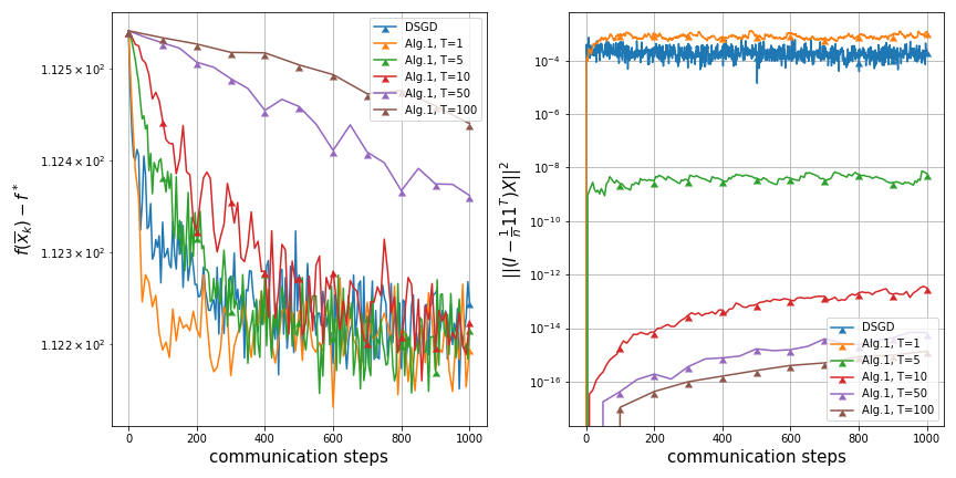
Figure 1: Random geometric graph with 20 nodes; batch size $r=10$

We observe a tradeoff between consensus accuracy and convergence speed in function value. A large number of consensus steps results in more accurate consensus and slower convergence, and vice versa. This tradeoff is present for different batch sizes.

VI Conclusion

We propose an accelerated distributed optimization algorithm for stochastic optimization problems in two settings: time-varying graphs and static graphs. For the latter setting we achieve the full acceleration and our method achieves lower bounds both for the communication and oracle per node complexity.

Our approach is based on accelerated gradient method with stochastic inexact oracle which makes it generic with many possible extensions. In particular, we focus on a specific case of strongly convex smooth functions, but the possible extensions include non-strongly convex and/or non-smooth functions that can be covered by such inexact oracles [64, 65]. Further, we believe that our results can be extended for composite optimization problems, zeroth-order optimization methods [66, 67, 68], and distributed algorithms for saddle-point problems [69] and variational inequalities.

APPENDIX

VI-A Proof of Lemma IV.1

Proof:

The first statement is proved in Lemma 2.1 of [61]. For the second statement, we have

$$\mathbb{E}\widetilde{g}_{\delta,L,\mu}(\overline{x},{\bf x}) =\frac{1}{n}\sum_{i=1}^{n}\frac{1}{r}\sum_{j=1}^{r}\mathbb{E}\nabla{\bf f}_{i}(x_{i},\xi_{i}^{j})=\frac{1}{n}\sum_{i=1}^{n}\frac{1}{r}\sum_{j=1}^{r}\nabla f_{i}(x_{i})=\frac{1}{n}\sum_{i=1}^{n}\nabla f_{i}(x_{i})=g_{\delta,L,\mu}(\overline{x},{\bf x}).$$

It remains to show (9b).

$$\mathbb{E}\left\|\widetilde{g}_{\delta,L,\mu}(\overline{x},{\bf x})-g_{\delta,L,\mu}(\overline{x},{\bf x})\right\|^{2}\leq\mathbb{E}\left\|\frac{1}{n}\sum_{i=1}^{n}\frac{1}{r}\sum_{j=1}^{r}\nabla{\bf f}_{i}(x_{i},\xi_{i}^{j})-\frac{1}{n}\sum_{i=1}^{n}\nabla f_{i}(x_{i})\right\|^{2}$$

$$\qquad\leq\frac{1}{n^{2}}\sum_{i=1}^{n}\mathbb{E}\left\|\frac{1}{r}\sum_{j=1}^{r}\nabla{\bf f}_{i}(x_{i},\xi_{i}^{j})-\nabla f_{i}(x_{i})\right\|^{2}\leq\frac{1}{n^{2}r^{2}}\sum_{i=1}^{n}\sum_{j=1}^{r}\mathbb{E}\left\|\nabla{\bf f}_{i}(x_{i},\xi_{i}^{j})-\nabla f_{i}(x_{i})\right\|^{2}$$

$$\qquad\leq\frac{\sum_{i=1}^{n}\sigma^{2}_{i}}{n^{2}r}{\color[rgb]{0,0,0}=\frac{\sigma_{g}^{2}}{nr}}.$$

The last inequality follows directly from (2). ∎

VI-B Proof of Theorem IV.2

For proving the theorem about complexity bounds, we need the following auxiliary Lemma:

Lemma VI.1

Let $\psi$ be convex function. Then for

$$y=\operatorname*{arg\,min}_{x\in Q}\left(\psi(x)+\beta\left\|x-z\right\|^{2}+\gamma\left\|x-u\right\|^{2}\right),$$ (17)

where $\beta>0$ and $\gamma>0$, the following is true for any $x\in Q$:

$$\psi(x)+\beta\left\|x-z\right\|^{2}+\gamma\left\|x-u\right\|^{2}\geq\psi(y)+\beta\left\|y-z\right\|^{2}+\gamma\left\|y-u\right\|^{2}+(\beta+\gamma)\left\|x-y\right\|^{2}.$$ (18)

Proof:

As $y$ is minimum, the subgradient of function at point $y$ includes $0$:

$$\exists g:g+\beta\nabla_{x}\left\|x-z\right\|^{2}|_{x=y}+\gamma\nabla_{x}\left\|x-u\right\|^{2}|_{x=y}=0.$$

It holds

$$\psi(x)-\psi(y) \geq\left\langle g,x-y\right\rangle=\left\langle\beta\nabla_{x}\left\|x-z\right\|^{2}|_{x=y}+\gamma\nabla_{x}\left\|x-u\right\|^{2}|_{x=y},y-x\right\rangle$$ (19)

$$=\left\langle 2\beta(y-z)+2\gamma(y-u),y-x\right\rangle$$ (20)

and we get that

$$2\left\langle y-z,y-x\right\rangle =\left\|y\right\|^{2}-\left\|z\right\|^{2}-2\left\langle z,y-z\right\rangle+\left\|x\right\|^{2}-\left\|y\right\|^{2}-2\left\langle y,x-y\right\rangle-\left\|x\right\|^{2}+\left\|z\right\|^{2}+2\left\langle z,x-z\right\rangle$$

$$=\left\|y-z\right\|^{2}+\left\|x-y\right\|^{2}-\left\|x-z\right\|^{2}.$$

After similar manipulations with the $2\left\langle y-u,y-x\right\rangle$ term and replacing the right part in (19), the lemma statement is obtained. ∎

Now we pass to the proof of Theorem IV.2 itself.

Proof:

We begin from the right inequality from (IV-B):

$$f(y)-\left(f_{\delta_{k+1},L,\mu}(x)+\left\langle g_{\delta_{k+1},L,\mu}(x),y-x\right\rangle\right)\leq\frac{L}{2}\left\|y-x\right\|^{2}+\delta_{k+1}.$$

It can be rewritten as

$$f(x^{k+1}) -\left(f_{\delta_{k+1},L,\mu}(y^{k+1})+\left\langle\widetilde{g}^{\ r_{k+1}}_{\delta_{k+1},L,\mu}(y^{k+1}),x^{k+1}-y^{k+1}\right\rangle\right)$$

$$\leq\left\langle g_{\delta_{k+1},L,\mu}(y^{k+1})-\widetilde{g}^{\ r_{k+1}}_{\delta_{k+1},L,\mu}(y^{k+1}),x^{k+1}-y^{k+1}\right\rangle+\frac{L}{2}\left\|y^{k+1}-x^{k+1}\right\|^{2}+\delta_{k+1}.$$

The first term in the right hand side can be estimated using Young inequality:

$$\left\langle g_{\delta_{k+1},L,\mu}(y^{k+1})-\widetilde{g}^{\ r_{k+1}}_{\delta_{k+1},L,\mu}(y^{k+1}),x^{k+1}-y^{k+1}\right\rangle\leq\frac{L}{2}\left\|x^{k+1}-y^{k+1}\right\|^{2}+\frac{1}{2L}\left\|g_{\delta_{k+1},L,\mu}(y^{k+1})-\widetilde{g}^{\ r_{k+1}}_{\delta_{k+1},L,\mu}(y^{k+1})\right\|^{2}$$

The combination of the last two expressions yields

$$f(x^{k+1})\leq f_{\delta_{k+1},L,\mu}(y^{k+1})+\left\langle\widetilde{g}^{\ r_{k+1}}_{\delta_{k+1},L,\mu}(y^{k+1}),x^{k+1}-y^{k+1}\right\rangle+L\left\|y^{k+1}-x^{k+1}\right\|^{2}+\lambda+\delta_{k+1},$$

where

$$\lambda:=\frac{1}{2L}\left\|g_{\delta_{k+1},L,\mu}(y^{k+1})-\widetilde{g}^{\ r_{k+1}}_{\delta_{k+1},L,\mu}(y^{k+1})\right\|^{2}$$

for brevity. We substitute $x^{k+1},y^{k+1}$ into several terms by their definitions:

$$f(x^{k+1})\leq f_{\delta_{k+1},L,\mu}(y^{k+1})+\left\langle\widetilde{g}^{\ r_{k+1}}_{\delta_{k+1},L,\mu}(y^{k+1}),\frac{\alpha^{k+1}u^{k+1}+A^{k}x^{k}}{A^{k+1}}-y^{k+1}\right\rangle$$

$$+L\left\|\frac{\alpha^{k+1}u^{k}+A^{k}x^{k}}{A^{k+1}}-\frac{\alpha^{k+1}u^{k+1}+A^{k}x^{k}}{A^{k+1}}\right\|^{2}+\lambda+\delta_{k+1}.$$

As $A^{k+1}=A^{k}+\alpha^{k+1}$ by definition and as dot product is convex, we get the following:

$$f(x^{k+1}) \leq\frac{A^{k}}{A^{k+1}}\left(f_{\delta_{k+1},L,\mu}(y^{k+1})+\left\langle\widetilde{g}^{\ r_{k+1}}_{\delta_{k+1},L,\mu}(y^{k+1}),x^{k}-y^{k+1}\right\rangle\right)$$

$$\quad+\frac{\alpha^{k+1}}{A^{k+1}}\left(f_{\delta_{k+1},L,\mu}(y^{k+1})+\left\langle\widetilde{g}^{\ r_{k+1}}_{\delta_{k+1},L,\mu}(y^{k+1}),u^{k+1}-y^{k+1}\right\rangle\right)+\frac{L(\alpha^{k+1})^{2}}{(A^{k+1})^{2}}\left\|u^{k}-u^{k+1}\right\|^{2}+\lambda+\delta_{k+1}.$$

By definition of $\alpha^{k+1}$ we have:

$$f(x^{k+1}) \leq\frac{A^{k}}{A^{k+1}}\left(f_{\delta_{k+1},L,\mu}(y^{k+1})+\left\langle\widetilde{g}^{\ r_{k+1}}_{\delta_{k+1},L,\mu}(y^{k+1}),x^{k}-y^{k+1}\right\rangle\right)$$

$$\quad+\frac{\alpha^{k+1}}{A^{k+1}}\left(f_{\delta_{k+1},L,\mu}(y^{k+1})+\left\langle\widetilde{g}^{\ r_{k+1}}_{\delta_{k+1},L,\mu}(y^{k+1}),u^{k+1}-y^{k+1}\right\rangle\right)+\frac{1+A^{k}\mu}{A^{k+1}}\left\|u^{k}-u^{k+1}\right\|^{2}+\lambda+\delta_{k+1}.$$

We rewrite that as:

$$f(x^{k+1}) \leq\frac{A^{k}}{A^{k+1}}\left(f_{\delta_{k+1},L,\mu}(y^{k+1})+\left\langle g_{\delta_{k+1},L,\mu}(y^{k+1}),x^{k}-y^{k+1}\right\rangle+\left\langle\widetilde{g}^{\ r_{k+1}}_{\delta_{k+1},L,\mu}(y^{k+1})-g_{\delta_{k+1},L,\mu}(y^{k+1}),x^{k}-y^{k+1}\right\rangle\right)$$

$$\quad+\frac{\alpha^{k+1}}{A^{k+1}}\left(f_{\delta_{k+1},L,\mu}(y^{k+1})+\left\langle\widetilde{g}^{\ r_{k+1}}_{\delta_{k+1},L,\mu}(y^{k+1}),u^{k+1}-y^{k+1}\right\rangle\right)+\frac{1+A^{k}\mu}{A^{k+1}}\left\|u^{k}-u^{k+1}\right\|^{2}+\lambda+\delta_{k+1}.$$

Using left part of (IV-B), we get:

$$f(x^{k+1}) \leq\frac{A^{k}}{A^{k+1}}\left(f(x^{k})+\left\langle\widetilde{g}^{\ r_{k+1}}_{\delta_{k+1},L,\mu}(y^{k+1})-g_{\delta_{k+1},L,\mu}(y^{k+1}),x^{k}-y^{k+1}\right\rangle\right)$$ (21)

$$+\frac{\alpha^{k+1}}{A^{k+1}}\left(f_{\delta_{k+1},L,\mu}(y^{k+1})+\left\langle\widetilde{g}^{\ r_{k+1}}_{\delta_{k+1},L,\mu}(y^{k+1}),u^{k+1}-y^{k+1}\right\rangle\right)+\frac{1+A^{k}\mu}{A^{k+1}}\left\|u^{k}-u^{k+1}\right\|^{2}+\lambda+\delta_{k+1}.$$ (22)

From lemma VI.1 for optimization problem at step 5 in Algorithm 3 we have:

$$\alpha^{k+1} \left\langle\widetilde{g}^{\ r_{k+1}}_{\delta_{k+1},L,\mu}(y^{k+1}),u^{k+1}-y^{k+1}\right\rangle+(1+A^{k}\mu)\left\|u^{k+1}-u^{k}\right\|^{2}+\alpha^{k+1}\mu\left\|u^{k+1}-y^{k+1}\right\|^{2}$$

$$+(1+A^{k}\mu+\alpha^{k+1}\mu)\left\|u^{k+1}-x\right\|^{2}\leq\alpha^{k+1}\left\langle\widetilde{g}^{\ r_{k+1}}_{\delta_{k+1},L,\mu}(y^{k+1}),x-y^{k+1}\right\rangle$$

$$+(1+A^{k}\mu)\left\|x-u^{k}\right\|^{2}+\alpha^{k+1}\mu\left\|x-y^{k+1}\right\|^{2}.$$

As squared norm is always non-negative, we obtain

$$\alpha^{k+1} \left\langle\widetilde{g}^{\ r_{k+1}}_{\delta_{k+1},L,\mu}(y^{k+1}),u^{k+1}-y^{k+1}\right\rangle+(1+A^{k}\mu)\left\|u^{k+1}-u^{k}\right\|^{2}\leq-(1+A^{k}\mu+\alpha^{k+1}\mu)\left\|u^{k+1}-x\right\|^{2}$$ (23)

$$+\alpha^{k+1}\left\langle\widetilde{g}^{\ r_{k+1}}_{\delta_{k+1},L,\mu}(y^{k+1}),x-y^{k+1}\right\rangle+(1+A^{k}\mu)\left\|x-u^{k}\right\|^{2}+\alpha^{k+1}\mu\left\|x-y^{k+1}\right\|^{2}$$ (24)

Combining inequalities (21) and (23), we get:

$$A^{k+1}f(x^{k+1})\leq\leavevmode\nobreak\ A^{k}\left(f(x^{k})+\left\langle\widetilde{g}^{\ r_{k+1}}_{\delta_{k+1},L,\mu}(y^{k+1})-g_{\delta_{k+1},L,\mu}(y^{k+1}),x^{k}-y^{k+1}\right\rangle\right)$$

$$+\alpha^{k+1}\left(f_{\delta_{k+1},L,\mu}(y^{k+1})+\left\langle\widetilde{g}^{\ r_{k+1}}_{\delta_{k+1},L,\mu}(y^{k+1}),x-y^{k+1}\right\rangle+\mu\left\|x-y^{k+1}\right\|^{2}\right)$$

$$+(1+A^{k}\mu)\left\|x-u^{k}\right\|^{2}-(1+A^{k}\mu+\alpha^{k+1}\mu)\left\|u^{k+1}-x\right\|^{2}+A^{k+1}\lambda+\delta_{k+1}A^{k+1}$$

$$=\leavevmode\nobreak\ A^{k}\left(f(x^{k})+\left\langle\widetilde{g}^{\ r_{k+1}}_{\delta_{k+1},L,\mu}(y^{k+1})-g_{\delta_{k+1},L,\mu}(y^{k+1}),x^{k}-y^{k+1}\right\rangle\right)$$

$$+\alpha^{k+1}\left(f_{\delta_{k+1},L,\mu}(y^{k+1})+\left\langle{g}_{\delta_{k+1},L,\mu}(y^{k+1}),x-y^{k+1}\right\rangle\right)$$

$$+\alpha^{k+1}\left(\left\langle\widetilde{g}^{\ r_{k+1}}_{\delta_{k+1},L,\mu}(y^{k+1})-{g}_{\delta_{k+1},L,\mu}(y^{k+1}),x-y^{k+1}\right\rangle+\mu\left\|x-y^{k+1}\right\|^{2}\right)$$

$$+(1+A^{k}\mu)\left\|x-u^{k}\right\|^{2}-(1+A^{k}\mu+\alpha^{k+1}\mu)\left\|u^{k+1}-x\right\|^{2}+A^{k+1}\lambda+\delta_{k+1}A^{k+1}.$$

Using the left part of (IV-B) again results in

$$A^{k+1}f(x^{k+1})\leq {A^{k}}\left(f(x^{k})+\left\langle\widetilde{g}^{\ r_{k+1}}_{\delta_{k+1},L,\mu}(y^{k+1})-g_{\delta_{k+1},L,\mu}(y^{k+1}),x^{k}-y^{k+1}\right\rangle\right)$$

$$+\alpha^{k+1}\left(f(x)+\left\langle\widetilde{g}^{\ r_{k+1}}_{\delta_{k+1},L,\mu}(y^{k+1})-{g}_{\delta_{k+1},L,\mu}(y^{k+1}),x-y^{k+1}\right\rangle+\right)$$

$$+(1+A^{k}\mu)\left\|x-u^{k}\right\|^{2}-(1+A^{k}\mu+\alpha^{k+1}\mu)\left\|u^{k+1}-x\right\|^{2}+A^{k+1}\lambda+\delta_{k+1}A^{k+1}.$$

We can take expectation and we may see that angles terms go zero as $\mathbb{E}\widetilde{g}^{\ r}_{\delta,L,\mu}(x)=g_{\delta,L,\mu}(x)$ for any $r$, and $\lambda\leq\frac{\sigma^{2}}{2Lr_{k+1}}$:

$$A^{k+1}\mathbb{E}f(x^{k+1}) -{A^{k}}f(x^{k})\leq\alpha^{k+1}f(x)$$

$$+(1+A^{k}\mu)\left\|x-u^{k}\right\|^{2}-(1+A^{k+1}\mu)\mathbb{E}\left\|u^{k+1}-x\right\|^{2}+\frac{\sigma^{2}A^{k+1}}{2Lr_{k+1}}+\delta_{k+1}A^{k+1}.$$

Now we should pay attention to the fact that the expectation is conditional because we consider $x^{k}$ and other $k$-th variables known before the iteration:

$$A^{k+1}\mathbb{E}\left[f(x^{k+1})|x^{k},\ldots,x^{1}\right] -{A^{k}}f(x^{k})\leq\alpha^{k+1}f(x)+(1+A^{k}\mu)\left\|x-u^{k}\right\|^{2}$$

$$-(1+A^{k+1}\mu)\mathbb{E}\left[\left\|u^{k+1}-x\right\|^{2}|x^{k},\ldots,x^{1}\right]+\frac{\sigma^{2}A^{k+1}}{2Lr_{k+1}}+\mathbb{E}[\delta_{k+1}|x^{k},\ldots,x^{1}]A^{k+1}.$$

If we take $x=x^{*}$, write these inequalities for all $k$ from $0$ to $N-1$ and sum up all of them, we will get the following:

$$\sum_{i=1}^{N}A^{i} \mathbb{E}\left[f(x^{i})|x^{i},\ldots,x^{1}\right]\leq\sum_{i=0}^{N-1}A^{i}f(x^{i})+\sum_{i=1}^{N}\alpha_{i}f(x^{*})+$$

$$+\sum_{i=0}^{N-1}(1+A^{i}\mu)\left\|u^{i}-x^{*}\right\|^{2}-\sum_{i=1}^{N}(1+A^{i}\mu)\mathbb{E}\left[\left\|u^{i}-x^{*}\right\|^{2}|x^{i},\ldots,x^{1}\right]+\sum_{i=1}^{N}A_{i}\left(\frac{\sigma^{2}}{2Lr_{i}}+\mathbb{E}[\delta_{i}|x^{i},\ldots,x^{1}]\right).$$

Next, we use the law of total expectation $N$ times and get rid of conditional expectations, and after that get rid of similar terms:

$$\mathbb{E}A^{N}f(x^{N})\leq A^{N}f(x^{*})+\left\|u^{0}-x^{*}\right\|^{2}-(1+A^{N}\mu)\mathbb{E}\left\|u^{N}-x^{*}\right\|^{2}+\sum_{i=1}^{N}A_{i}\left(\frac{\sigma^{2}}{2Lr_{i}}+\mathbb{E}\delta_{i}\right)$$ (25)

Here we also recall that $A_{0}=\alpha_{0}=0,\sum_{i=1}^{N}\alpha_{i}=A_{N}$.

Finally, we get

$$\mathbb{E}f(x^{N})-f(x^{*})\leq\frac{1}{A^{N}}\left(\left\|u^{0}-x^{*}\right\|^{2}+\sum_{i=1}^{N}A^{i}\left(\frac{\sigma^{2}}{2Lr_{i}}+\mathbb{E}\delta_{i}\right)\right).$$

The second inequality is obtained from (25) and the fact that $f(x)\geq f(x^{*})$. ∎

VI-C Proof of Lemma IV.3

Proof:

In view of definition of sequence $\alpha^{k+1}$, we have:

$$A^{N} \leq A^{N}(1+\mu A^{N-1})=L(A^{N}-A^{N-1})^{2}$$

$$\leq L(\sqrt{A^{N}}-\sqrt{A^{N-1}})^{2}(\sqrt{A^{N}}+\sqrt{A^{N-1}})^{2}\leq 4L^{N}A^{N}(\sqrt{A^{N}}-\sqrt{A^{N-1}})^{2}.$$

For the case when $\mu>0$ we obtain:

$$\mu A^{N-1}A^{N}\leq A^{N}(1+\mu A^{N-1})\leq 4LA^{N}(\sqrt{A^{N}}-\sqrt{A^{N-1}})^{2}.$$

From the fact that $A^{1}=1/L$ and the last inequality we can show that

$$\sqrt{A^{N}}\geq\left(1+\frac{1}{2}\sqrt{\frac{\mu}{L}}\right)\sqrt{A^{N-1}}\geq\frac{1}{\sqrt{L}}\left(1+\frac{1}{2}\sqrt{\frac{\mu}{L}}\right)^{(N-1)}.$$

For the second statement, we recall the proof of Lemma A.1 in [61]. Update rule for $A^{k}$ writes as

$$1+\mu A^{k}=\frac{L(\alpha^{k+1})^{2}}{A^{k+1}},\leavevmode\nobreak\ A^{k}=\sum_{i=0}^{k}\alpha^{i},\leavevmode\nobreak\ \alpha^{0}=0.$$ (26)

A sequence $\left\{B^{k}\right\}_{k=0}^{\infty}$ with a similar update rule is studied in [58].

$$L+\mu B^{k}=\frac{L(\beta^{k+1})^{2}}{B^{k+1}},\leavevmode\nobreak\ B^{k}=\sum_{i=0}^{k}\beta^{i},\leavevmode\nobreak\ \beta^{0}=1,$$ (27)

and for sequence $\left\{B^{k}\right\}_{k=0}^{\infty}$ it is shown $\frac{\sum_{i=0}^{k}B^{i}}{B^{k}}\leq 1+\sqrt{L/\mu}$. Dividing (27) by L yields

$$1+\mu(B^{k}/L)=\frac{L(\beta^{k+1}/L)^{2}}{(B^{k+1}/L)},$$

which means that update rule for $B^{k}/L$ is equivalent to (26). Since $A^{1}=1/L=B^{0}/L$, it holds $A^{k+1}=B^{k}/L,\leavevmode\nobreak\ k\geq 0$ and

$$\frac{\sum_{i=1}^{k}A^{i}}{A^{k}}=\frac{\sum_{i=0}^{k-1}B^{i}/L}{B^{k-1}/L}\leq 1+\sqrt{\frac{L}{\mu}}.$$

∎

VI-D Proof of Lemma IV.5

Proof:

The proof follows by revisiting proof of Lemma A.3 in [61] in stochastic setting. First, note that multiplication by a mixing matrix does not change the average of a vector, i.e. $\frac{1}{n}\mathbf{1}_{n}\mathbf{1}_{n}^{\top}{\bf x}=\frac{1}{n}\mathbf{1}_{n}\mathbf{1}_{n}^{\top}{\bf W}^{k}{\bf x}\leavevmode\nobreak\ \forall k\geq 0$. This means $\overline{\bf u}^{k+1}=\overline{\bf v}^{k+1}$.

Second, let us use the contraction property of mixing matrix sequence $\{{\bf W}^{k}\}_{k=0}^{\infty}$. We have

$$\mathbb{E}\left\|{\bf u}^{k+1}-\overline{\bf u}^{k+1}\right\|^{2} \leq(1-\lambda)^{2(T/\tau)}\mathbb{E}\left\|{\bf v}^{k+1}-\overline{\bf u}^{k+1}\right\|^{2}\leq e^{-2(T/\tau)\lambda}\mathbb{E}\left\|{\bf v}^{k+1}-\overline{\bf u}^{k+1}\right\|^{2}.$$

Assuming that $\mathbb{E}\left\|{\bf v}^{k+1}-\overline{\bf u}^{k+1}\right\|^{2}\leq D$, we only need $T=\frac{\tau}{2\lambda}\log\frac{D}{\delta^{\prime}}$ iterations to ensure $\mathbb{E}\left\|{\bf u}^{k+1}-\overline{\bf u}^{k+1}\right\|^{2}\leq\delta^{\prime}$. In the rest of the proof, we show that $\mathbb{E}\left\|{\bf v}^{k+1}-\overline{\bf u}^{k+1}\right\|=\mathbb{E}\left\|{\bf v}^{k+1}-\overline{\bf v}^{k+1}\right\|\leq\sqrt{D}$.

According to update rule of Algorithm 1, it holds

$$\mathbb{E}\left\|{\bf v}^{k+1}-\overline{\bf v}^{k+1}\right\| \leq\frac{\alpha^{k+1}\mu\mathbb{E}\left\|{\bf y}^{k+1}-\overline{\bf y}^{k+1}\right\|}{1+A^{k+1}\mu}+\frac{(1+A^{k}\mu)\mathbb{E}\left\|{\bf u}^{k}-\overline{\bf u}^{k}\right\|}{1+A^{k+1}\mu}+\frac{\alpha^{k+1}}{1+A^{k+1}\mu}\mathbb{E}\left\|\nabla^{r}F({\bf y}^{k+1})\right\|$$

$$\leq\sqrt{\delta^{\prime}}+\frac{\alpha^{k+1}}{1+A^{k+1}\mu}\mathbb{E}\left\|\nabla^{r}F({\bf y}^{k+1})\right\|.$$

We estimate $\left\|\nabla^{r}F({\bf y}^{k+1})\right\|$ using $L_{\xi}$-smoothness of $\nabla F$:

$$\left\|\nabla^{r}F({\bf y}^{k+1})\right\| \leq\left\|\nabla^{r}F({\bf y}^{k+1})-\nabla^{r}F({\bf x}^{*})\right\|+\left\|\nabla^{r}F({\bf x}^{*})\right\|$$

$$\leq L_{\xi}\underbrace{\left\|{\bf y}^{k+1}-\overline{\bf y}^{k+1}\right\|}_{\leq\sqrt{\delta^{\prime}}}+L_{\xi}\underbrace{\left\|\overline{\bf y}^{k+1}-{\bf x}^{*}\right\|}_{=\sqrt{n}\left\|\overline{y}^{k+1}-x^{*}\right\|}+\left\|\nabla^{r}F({\bf x}^{*})\right\|$$ (28)

where $x^{*}=\operatorname*{arg\,min}_{x\in\mathbb{R}^{d}}f(x),\leavevmode\nobreak\ {\bf x}^{*}=\mathbf{1}_{n}(x^{*})^{\top}$. It remains to estimate $\left\|\overline{y}^{k+1}-x^{*}\right\|$.

$$\left\|\overline{y}^{k+1}-x^{*}\right\| \leq\frac{\alpha^{k+1}}{A^{k+1}}\left\|\overline{x}^{k+1}-x^{*}\right\|+\frac{A^{k}}{A^{k+1}}\left\|\overline{u}^{k+1}-x^{*}\right\|\leq\max\left\{\left\|\overline{x}^{k+1}-x^{*}\right\|,\left\|\overline{u}^{k+1}-x^{*}\right\|\right\}$$

By Lemma IV.4 and strong convexity of $f$:

$$\mathbb{E}\left\|\overline{x}^{k+1}-x^{*}\right\|^{2} \leq\frac{2}{\mu}\left(\mathbb{E}f(\overline{x}^{k+1})-f(x^{*})\right)\leq\frac{\left\|\overline{u}^{0}-x^{*}\right\|^{2}}{A^{k+1}\mu}+\frac{\sum_{i=1}^{k+1}A^{i}}{A^{k+1}\mu}\left(\frac{\sigma^{2}}{2Lr}+\delta\right)$$

and therefore

$$\mathbb{E}\left\|\overline{y}^{k+1}-x^{*}\right\|^{2} \leq\max\left\{\frac{\left\|\overline{u}^{0}-x^{*}\right\|^{2}}{A^{k+1}\mu}+\frac{\sum_{i=1}^{k+1}A^{i}}{A^{k+1}\mu}\left(\frac{\sigma^{2}}{2Lr}+\delta\right),\leavevmode\nobreak\ \frac{\left\|\overline{u}^{0}-x^{*}\right\|^{2}}{1+A^{k+1}\mu}+\frac{\sum_{i=1}^{k+1}A^{i}}{1+A^{k+1}\mu}\left(\frac{\sigma^{2}}{2Lr}+\delta\right)\right\}$$

$$\leq\frac{\left\|\overline{u}^{0}-x^{*}\right\|^{2}}{A^{k+1}\mu}+\frac{1}{\mu}\left(1+\sqrt{\frac{L}{\mu}}\right)\left(\frac{\sigma^{2}}{2Lr}+\delta\right),$$

where the last inequality holds by Lemma IV.3.

Returning to (28), we get

$$\left\|\nabla^{r}F({\bf y}^{k+1})\right\|$$

$$\qquad\leq L_{\xi}\sqrt{\delta^{\prime}}+L_{\xi}\sqrt{n}\left(\frac{\left\|\overline{u}^{0}-x^{*}\right\|^{2}}{A^{k+1}\mu}+\frac{1}{\mu}\left(1+\sqrt{\frac{L}{\mu}}\right)\left(\frac{\sigma^{2}}{2Lr}+\delta\right)\right)^{1/2}+\left\|\nabla^{r}F({\bf x}^{*})\right\|$$

$$\qquad\leq L_{\xi}\sqrt{\delta^{\prime}}+L_{\xi}\sqrt{n}\left(\frac{L}{\mu}\left\|\overline{u}^{0}-x^{*}\right\|^{2}\left(1+\sqrt{\frac{\mu}{2L}}\right)^{-2k}+\frac{2L^{1/2}}{\mu^{3/2}}\left(\frac{\sigma^{2}}{2Lr}+\delta\right)\right)^{1/2}+\left\|\nabla^{r}F({\bf x}^{*})\right\|$$

$$\qquad\leq L_{\xi}\sqrt{\delta^{\prime}}+L_{\xi}\sqrt{n}\left(\frac{L}{\mu}\left\|\overline{u}^{0}-x^{*}\right\|^{2}+\frac{2L^{1/2}}{\mu^{3/2}}\left(\frac{\sigma^{2}}{2Lr}+\delta\right)\right)^{1/2}+\left\|\nabla^{r}F({\bf x}^{*})\right\|.$$

For distance to consensus of ${\bf v}^{k+1}$, it holds

$$\mathbb{E}\left\|{\bf v}^{k+1}-\overline{\bf v}^{k+1}\right\|\leq\sqrt{\delta^{\prime}}+\frac{\alpha^{k+1}}{1+A^{k}\mu+\mu}\mathbb{E}\left\|\nabla F\left({\bf y}^{k+1}\right)\right\|$$

We estimate coefficient by $\mathbb{E}\left\|\nabla F\left({\bf y}^{k+1}\right)\right\|$ using the definition of $\alpha^{k+1}$.

$$1+A^{k}\mu=\frac{L(\alpha^{k+1})^{2}}{A^{k}+\alpha^{k+1}}$$

$$L(\alpha^{k+1})^{2}-(1+A^{k}\mu)\alpha^{k+1}-(1+A^{k}\mu)A^{k}=0$$

$$\alpha^{k+1}=\frac{1+A^{k}\mu+\sqrt{(1+A^{k}\mu)^{2}+4LA^{k}(1+A^{k}\mu)}}{2L}$$

$$\frac{\alpha^{k+1}}{1+A^{k+1}\mu}\leq\frac{\alpha^{k+1}}{1+A^{k}\mu}=\frac{1}{2L}\left(1+\sqrt{1+4\frac{LA^{k}}{1+A^{k}\mu}}\right)$$

$$\qquad\leq\frac{1}{2L}\left(\sqrt{\frac{L}{\mu}}+\sqrt{\frac{L}{\mu}+4\frac{L}{\mu}}\right)\leq\frac{2}{\sqrt{L\mu}}$$

Returning to ${\bf v}^{k+1}$, we get

$$\mathbb{E}\left\|{\bf v}^{k+1}-\overline{\bf v}^{k+1}\right\|$$

$$\qquad\leq\left(\frac{2L_{l}}{\sqrt{L\mu}}+1\right)\sqrt{\delta^{\prime}}+L_{l}\sqrt{\frac{n}{L\mu}}\left(\frac{L}{\mu}\left\|\overline{u}^{0}-x^{*}\right\|^{2}+\frac{2L^{1/2}}{\mu^{3/2}}\left(\frac{\sigma^{2}}{2Lr}+\delta\right)\right)^{1/2}+\frac{2\mathbb{E}\left\|\nabla^{r}F({\bf x}^{*})\right\|}{\sqrt{L\mu}}$$

$$\qquad\leq\left(\frac{2L_{l}}{\sqrt{L_{g}\mu_{g}}}+1\right)\sqrt{\delta^{\prime}}+\frac{2L_{l}}{\mu_{g}}\sqrt{n}\left(\left\|\overline{u}^{0}-x^{*}\right\|^{2}+\frac{2}{\sqrt{L_{g}\mu_{g}}}\left(\frac{\sigma_{g}^{2}}{4nL_{g}r^{2}}+\delta\right)\right)^{1/2}+\frac{2nM_{\xi}}{\sqrt{L_{g}\mu_{g}}}=\sqrt{D},$$

where in the last inequality we used $\left\|\nabla^{r}F({\bf x}^{*})\right\|\leq nM_{\xi}$. ∎

VI-E Putting the proof of Theorem III.1 together

Let us show that choice of number of subroutine iterations $T_{k}=T$ yields

$$\mathbb{E}f(\overline{x}^{k})-f(x^{*})\leq\frac{1}{A^{k}}\left(\left\|\overline{u}^{0}-x^{*}\right\|^{2}+\left(\frac{\sigma^{2}}{2Lr}+\delta\right)\sum_{i=1}^{k}A^{i}\right)$$

by induction. At $k=0$, we have $\left\|{\bf u}^{0}-\overline{\bf u}^{0}\right\|=0$ and by Lemma IV.4 it holds

$$\mathbb{E}f(\overline{x}^{1})-f(x^{*}) \leq\frac{1}{A^{1}}\left(\left\|\overline{u}^{0}-x^{*}\right\|^{2}+\left(\frac{\sigma^{2}}{2Lr}+\delta\right)A^{1}\right).$$

For induction pass, assume that $\mathbb{E}\left\|{\bf u}^{j}-\overline{\bf u}^{j}\right\|^{2}\leq\delta^{\prime}$ for $j=0,\ldots,k$. By Lemma IV.5, if we set $T_{k}=T$, then $\mathbb{E}\left\|{\bf u}^{k+1}-\overline{\bf u}^{k+1}\right\|^{2}\leq\delta^{\prime}$. Applying Lemma IV.4 again, we get

$$\mathbb{E}f(\overline{x}^{k})-f(x^{*})\leq\frac{1}{A^{k}}\left(\left\|\overline{u}^{0}-x^{*}\right\|^{2}+\left(\frac{\sigma^{2}}{2Lr}+\delta\right)\sum_{i=1}^{k}A^{i}\right).$$

Next, we substitute a bound on $A^{k}$ from Lemma IV.3 and get

$$\mathbb{E}f(\overline{x}^{N}) -f(x^{*})$$

$$\leavevmode\nobreak\ \leq LR^{2}\left(1+\frac{1}{2}\sqrt{\frac{\mu}{L}}\right)^{-2(N-1)}+\left(1+\sqrt{\frac{L}{\mu}}\right)\left(\frac{\sigma^{2}}{2Lr}+\delta\right)$$

$$\leavevmode\nobreak\ =2L_{g}R^{2}\left(1+\frac{1}{4}\sqrt{\frac{\mu_{g}}{L_{g}}}\right)^{-2(N-1)}+\left(1+2\sqrt{\frac{L_{g}}{\mu_{g}}}\right)\left(\frac{\sigma^{2}}{4L_{g}r}+\delta\right).$$

It remains to estimate the number of iterations required for $\varepsilon$-accuracy. In order to satisfy

$$2L_{g}\left\|\overline{u}^{0}-x^{*}\right\|^{2}\left(1+\frac{1}{4}\sqrt{\frac{\mu_{g}}{L_{g}}}\right)^{-2(N-1)} \leq\frac{\varepsilon}{2},$$

$$\left(1+2\sqrt{\frac{L_{g}}{\mu_{g}}}\right)\left(\frac{\sigma^{2}}{4L_{g}r}+\delta\right) \leq\frac{\varepsilon}{2},$$

it is sufficient to choose $\delta^{\prime}=\dfrac{n\varepsilon}{32}\dfrac{\mu_{g}^{3/2}}{L_{g}^{1/2}L_{l}^{2}},\leavevmode\nobreak\ r=\dfrac{2\sigma^{2}}{\varepsilon\sqrt{L_{g}\mu_{g}}}$ and

$$N=3\sqrt{\frac{L_{g}}{\mu_{g}}}\log\left(\frac{4L_{g}\left\|\overline{u}^{0}-x^{*}\right\|^{2}}{\varepsilon}\right).$$

Finally, the total number of stochastic oracle calls per node equals

$$N_{orcl}=N\cdot r=\dfrac{6\sigma_{g}^{2}}{n\mu_{g}\varepsilon}\log\left(\frac{4L_{g}\left\|\overline{u}^{0}-x^{*}\right\|^{2}}{\varepsilon}\right).$$

Further, the total number of communications is

$$N_{\text{comm}} =N\cdot T=3\sqrt{\frac{L_{g}}{\mu_{g}}}\log\left(\frac{4L_{g}\left\|\overline{u}^{0}-x^{*}\right\|^{2}}{\varepsilon}\right)\cdot\kappa\cdot\log\frac{D}{\delta^{\prime}}$$

$$=O\left(\sqrt{\frac{L_{g}}{\mu_{g}}}\kappa\cdot\log\left(\frac{4L_{g}\left\|\overline{u}^{0}-x^{*}\right\|^{2}}{\varepsilon}\right)\log\frac{D}{\delta^{\prime}}\right),$$

where $\kappa=\frac{\tau}{2\lambda}$ if the communication network is time-varying and $\kappa=\sqrt{\chi}$ if the communication network is fixed.

References

- [1] V. Borkar and P. P. Varaiya, “Asymptotic agreement in distributed estimation,” IEEE Transactions on Automatic Control, vol. 27, no. 3, pp. 650–655, 1982.
- [2] J. N. Tsitsiklis and M. Athans, “Convergence and asymptotic agreement in distributed decision problems,” IEEE Transactions on Automatic Control, vol. 29, no. 1, pp. 42–50, 1984.
- [3] M. H. DeGroot, “Reaching a consensus,” Journal of the American Statistical Association, vol. 69, no. 345, pp. 118–121, 1974.
- [4] L. Xiao and S. Boyd, “Optimal scaling of a gradient method for distributed resource allocation,” Journal of Optimization Theory and Applications, vol. 129, no. 3, pp. 469–488, 2006.
- [5] M. Rabbat and R. Nowak, “Decentralized source localization and tracking wireless sensor networks,” in Proceedings of the IEEE International Conference on Acoustics, Speech, and Signal Processing, vol. 3, 2004, pp. 921–924.
- [6] S. S. Ram, V. V. Veeravalli, and A. Nedic, “Distributed non-autonomous power control through distributed convex optimization,” in IEEE INFOCOM 2009. IEEE, 2009, pp. 3001–3005.
- [7] T. Kraska, A. Talwalkar, J. C. Duchi, R. Griffith, M. J. Franklin, and M. I. Jordan, “Mlbase: A distributed machine-learning system.” in CIDR, vol. 1, 2013, pp. 2–1.
- [8] A. Nedić, A. Olshevsky, and C. A. Uribe, “Distributed learning for cooperative inference,” arXiv preprint arXiv:1704.02718, 2017.
- [9] ——, “Fast convergence rates for distributed non-bayesian learning,” IEEE Transactions on Automatic Control, vol. 62, no. 11, pp. 5538–5553, 2017.
- [10] C. A. Uribe, D. Dvinskikh, P. Dvurechensky, A. Gasnikov, and A. Nedić, “Distributed computation of Wasserstein barycenters over networks,” in 2018 IEEE Conference on Decision and Control (CDC), 2018, pp. 6544–6549.
- [11] A. Kroshnin, N. Tupitsa, D. Dvinskikh, P. Dvurechensky, A. Gasnikov, and C. Uribe, “On the complexity of approximating Wasserstein barycenters,” in Proceedings of the 36th International Conference on Machine Learning. PMLR, 2019, pp. 3530–3540.
- [12] A. Ivanova, P. Dvurechensky, A. Gasnikov, and D. Kamzolov, “Composite optimization for the resource allocation problem,” Optimization Methods and Software, 2020. [Online]. Available: https://doi.org/10.1080/10556788.2020.1712599
- [13] L. Bottou, “Large-scale machine learning with stochastic gradient descent,” in Proceedings of COMPSTAT’2010. Springer, 2010, pp. 177–186.
- [14] S. Boyd, N. Parikh, E. Chu, B. Peleato, and J. Eckstein, “Distributed optimization and statistical learning via the alternating direction method of multipliers,” Foundations and Trends® in Machine Learning, vol. 3, no. 1, pp. 1–122, 2011.
- [15] M. Abadi, A. Agarwal, P. Barham, E. Brevdo, Z. Chen, C. Citro, G. S. Corrado, A. Davis, J. Dean, M. Devin, et al., “Tensorflow: Large-scale machine learning on heterogeneous distributed systems.” in Conf. on Language Resources and Evaluation (LREC’08), 2016, pp. 3243–3249.
- [16] A. Nedić, A. Olshevsky, and W. Shi, “Achieving geometric convergence for distributed optimization over time-varying graphs,” SIAM Journal on Optimization, vol. 27, no. 4, pp. 2597–2633, 2017.
- [17] A. Nedić, A. Olshevsky, and C. A. Uribe, “Fast convergence rates for distributed non-Bayesian learning,” IEEE Transactions on Automatic Control, vol. 62, no. 11, pp. 5538–5553, Nov 2017.
- [18] A. Nedić, A. Olshevsky, A. Ozdaglar, and J. N. Tsitsiklis, “On distributed averaging algorithms and quantization effects,” IEEE Transactions on Automatic Control, vol. 54, no. 11, pp. 2506–2517, 2009.
- [19] S. S. Ram, A. Nedić, and V. V. Veeravalli, “Distributed stochastic subgradient projection algorithms for convex optimization,” Journal of Optimization Theory and Applications, vol. 147, no. 3, pp. 516–545, 2010.
- [20] A. Daneshmand, G. Scutari, P. Dvurechensky, and A. Gasnikov, “Newton method over networks is fast up to the statistical precision,” in Proceedings of the 38th International Conference on Machine Learning, vol. 139. PMLR, 2021, pp. 2398–2409.
- [21] K. Scaman, F. Bach, S. Bubeck, Y. T. Lee, and L. Massoulié, “Optimal algorithms for smooth and strongly convex distributed optimization in networks,” in International Conference on Machine Learning, 2017, pp. 3027–3036.
- [22] S. Ghadimi and G. Lan, “Optimal stochastic approximation algorithms for strongly convex stochastic composite optimization, ii: Shrinking procedures and optimal algorithms,” SIAM Journal on Optimization, vol. 23, no. 4, pp. 2061–2089, 2013.
- [23] P. E. Dvurechensky, A. V. Gasnikov, and A. A. Lagunovskaya, “Parallel algorithms and probability of large deviation for stochastic convex optimization problems,” Numerical Analysis and Applications, vol. 11, no. 1, pp. 33–37, 2018.
- [24] Y. Zhang and L. Xiao, Communication-Efficient Distributed Optimization of Self-concordant Empirical Loss. Cham: Springer International Publishing, 2018, pp. 289–341.
- [25] P. Dvurechensky, D. Kamzolov, A. Lukashevich, S. Lee, E. Ordentlich, C. A. Uribe, and A. Gasnikov, “Hyperfast second-order local solvers for efficient statistically preconditioned distributed optimization,” arXiv:2102.08246, 2021.
- [26] A. Agafonov, P. Dvurechensky, G. Scutari, A. Gasnikov, D. Kamzolov, A. Lukashevich, and A. Daneshmand, “An accelerated second-order method for distributed stochastic optimization,” in 2021 60th IEEE Conference on Decision and Control (CDC), 2021.
- [27] D. Dvinskikh and A. Gasnikov, “Decentralized and parallel primal and dual accelerated methods for stochastic convex programming problems,” Journal of Inverse and Ill-posed Problems, vol. 29, no. 3, pp. 385–405, 2021.
- [28] A. Nemirovskii and Yudin, Problem Complexity and Method Efficiency in Optimization. Wiley, 1983.
- [29] Y. Nesterov, “A method of solving a convex programming problem with convergence rate ,” Soviet Mathematics Doklady, vol. 27, no. 2, pp. 372–376, 1983.
- [30] Y. Nesterov, A. Gasnikov, S. Guminov, and P. Dvurechensky, “Primal-dual accelerated gradient methods with small-dimensional relaxation oracle,” Optimization Methods and Software, pp. 1–28, 2020. [Online]. Available: https://doi.org/10.1080/10556788.2020.1731747
- [31] S. V. Guminov, Y. E. Nesterov, P. E. Dvurechensky, and A. V. Gasnikov, “Accelerated primal-dual gradient descent with linesearch for convex, nonconvex, and nonsmooth optimization problems,” Doklady Mathematics, vol. 99, no. 2, pp. 125–128, 2019.
- [32] A. Fallah, M. Gurbuzbalaban, A. Ozdaglar, U. Simsekli, and L. Zhu, “Robust distributed accelerated stochastic gradient methods for multi-agent networks,” arXiv preprint arXiv:1910.08701, 2019.
- [33] D. Dvinskikh, E. Gorbunov, A. Gasnikov, P. Dvurechensky, and C. A. Uribe, “On primal and dual approaches for distributed stochastic convex optimization over networks,” in 2019 IEEE 58th Conference on Decision and Control (CDC), 2019, pp. 7435–7440.
- [34] A. Olshevsky, I. C. Paschalidis, and S. Pu, “Asymptotic network independence in distributed optimization for machine learning,” arXiv preprint arXiv:1906.12345, 2019.
- [35] ——, “A non-asymptotic analysis of network independence for distributed stochastic gradient descent,” arXiv:1906.02702, 2019.
- [36] A. Nedic and A. Ozdaglar, “Distributed subgradient methods for multi-agent optimization,” IEEE Transactions on Automatic Control, vol. 54, no. 1, pp. 48–61, 2009.
- [37] W. Shi, Q. Ling, G. Wu, and W. Yin, “Extra: An exact first-order algorithm for decentralized consensus optimization,” SIAM Journal on Optimization, vol. 25, no. 2, pp. 944–966, 2015.
- [38] A. Rogozin and A. Gasnikov, “Projected gradient method for decentralized optimization over time-varying networks,” arXiv:1911.08527, 2019.
- [39] G. Qu and N. Li, “Accelerated distributed nesterov gradient descent,” 2016 54th Annual Allerton Conference on Communication, Control, and Computing, 2016.
- [40] H. Ye, L. Luo, Z. Zhou, and T. Zhang, “Multi-consensus decentralized accelerated gradient descent,” arXiv preprint arXiv:2005.00797, 2020.
- [41] H. Li, C. Fang, W. Yin, and Z. Lin, “A sharp convergence rate analysis for distributed accelerated gradient methods,” arXiv:1810.01053, 2018.
- [42] D. Jakovetic, “A unification and generalization of exact distributed first order methods,” IEEE Transactions on Signal and Information Processing over Networks, pp. 31–46, 2019.
- [43] P. Dvurechenskii, D. Dvinskikh, A. Gasnikov, C. Uribe, and A. Nedich, “Decentralize and randomize: Faster algorithm for wasserstein barycenters,” in Advances in Neural Information Processing Systems 31, 2018, pp. 10 783–10 793.
- [44] H. Li and Z. Lin, “Revisiting extra for smooth distributed optimization,” arXiv preprint arXiv:2002.10110, 2020.
- [45] H. Hendrikx, F. Bach, and L. Massoulie, “An optimal algorithm for decentralized finite sum optimization,” arXiv:2005.10675, 2020.
- [46] H. Li, Z. Lin, and Y. Fang, “Optimal accelerated variance reduced extra and diging for strongly convex and smooth decentralized optimization,” arXiv preprint arXiv:2009.04373, 2020.
- [47] J. Tang, K. Egiazarian, M. Golbabaee, and M. Davies, “The practicality of stochastic optimization in imaging inverse problems,” arXiv:1910.10100, 2019.
- [48] X. Wu and J. Lu, “Fenchel dual gradient methods for distributed convex optimization over time-varying networks,” in 2017 IEEE 56th Annual Conference on Decision and Control (CDC), 2017, pp. 2894–2899.
- [49] G. Zhang and R. Heusdens, “Distributed optimization using the primal-dual method of multipliers,” IEEE Transactions on Signal and Information Processing over Networks, vol. 4, no. 1, pp. 173–187, 2018.
- [50] C. A. Uribe, S. Lee, A. Gasnikov, and A. Nedić, “A dual approach for optimal algorithms in distributed optimization over networks,” Optimization Methods and Software, pp. 1–40, 2020.
- [51] A. Nedić, A. Olshevsky, and W. Shi, “Achieving geometric convergence for distributed optimization over time-varying graphs,” SIAM Journal on Optimization, vol. 27, no. 4, pp. 2597–2633, 2017.
- [52] S. Pu, W. Shi, J. Xu, and A. Nedich, “A push-pull gradient method for distributed optimization in networks,” 2018 IEEE Conference on Decision and Control (CDC), pp. 3385–3390, 2018.
- [53] M. Maros and J. Jaldén, “Panda: A dual linearly converging method for distributed optimization over time-varying undirected graphs,” 2018 IEEE Conference on Decision and Control (CDC), pp. 6520–6525, 2018.
- [54] A. Koloskova, N. Loizou, S. Boreiri, M. Jaggi, and S. U. Stich, “A unified theory of decentralized sgd with changing topology and local updates,” arXiv preprint arXiv:2003.10422, 2020.
- [55] A. Wien, Iterative solution of large linear systems. Lecture Notes, TU Wien, 2011.
- [56] K. Scaman, F. Bach, S. Bubeck, L. Massoulié, and Y. T. Lee, “Optimal algorithms for non-smooth distributed optimization in networks,” in Advances in Neural Information Processing Systems, 2018, pp. 2740–2749.
- [57] F. Stonyakin, A. Tyurin, A. Gasnikov, P. Dvurechensky, A. Agafonov, D. Dvinskikh, M. Alkousa, D. Pasechnyuk, S. Artamonov, and V. Piskunova, “Inexact model: A framework for optimization and variational inequalities,” Optimization Methods and Software, 2021. [Online]. Available: https://doi.org/10.1080/10556788.2021.1924714
- [58] O. Devolder, F. Glineur, and Y. Nesterov, “First-order methods with inexact oracle: the strongly convex case,” CORE DP 2013/16, 2013.
- [59] P. Dvurechensky and A. Gasnikov, “Stochastic intermediate gradient method for convex problems with stochastic inexact oracle,” Journal of Optimization Theory and Applications, vol. 171, no. 1, pp. 121–145, 2016.
- [60] A. V. Gasnikov and P. E. Dvurechensky, “Stochastic intermediate gradient method for convex optimization problems,” Doklady Mathematics, vol. 93, no. 2, pp. 148–151, Mar 2016.
- [61] A. Rogozin, V. Lukoshkin, A. Gasnikov, D. Kovalev, and E. Shulgin, “Towards accelerated rates for distributed optimization over time-varying networks,” arXiv preprint arXiv:2009.11069, 2020.
- [62] F. S. Stonyakin, D. Dvinskikh, P. Dvurechensky, A. Kroshnin, O. Kuznetsova, A. Agafonov, A. Gasnikov, A. Tyurin, C. A. Uribe, D. Pasechnyuk, and S. Artamonov, “Gradient methods for problems with inexact model of the objective,” in Mathematical Optimization Theory and Operations Research, M. Khachay, Y. Kochetov, and P. Pardalos, Eds. Cham: Springer International Publishing, 2019, pp. 97–114.
- [63] C.-C. Chang and C.-J. Lin, “Libsvm: a library for support vector machines,” ACM transactions on intelligent systems and technology (TIST), vol. 2, no. 3, p. 27, 2011.
- [64] O. Devolder, F. Glineur, and Y. Nesterov, “First-order methods of smooth convex optimization with inexact oracle,” Mathematical Programming, vol. 146, no. 1-2, pp. 37–75, 2014.
- [65] D. Kamzolov, P. Dvurechensky, and A. V. Gasnikov, “Universal intermediate gradient method for convex problems with inexact oracle,” Optimization Methods and Software, 2020. [Online]. Available: https://doi.org/10.1080/10556788.2019.1711079
- [66] E. Gorbunov, P. Dvurechensky, and A. Gasnikov, “An accelerated method for derivative-free smooth stochastic convex optimization,” arXiv:1802.09022, 2018.
- [67] E. A. Vorontsova, A. V. Gasnikov, E. A. Gorbunov, and P. E. Dvurechenskii, “Accelerated gradient-free optimization methods with a non-euclidean proximal operator,” Automation and Remote Control, vol. 80, no. 8, pp. 1487–1501, 2019.
- [68] P. Dvurechensky, E. Gorbunov, and A. Gasnikov, “An accelerated directional derivative method for smooth stochastic convex optimization,” European Journal of Operational Research, vol. 290, no. 2, pp. 601 – 621, 2021.
- [69] A. V. Gasnikov, D. M. Dvinskikh, P. E. Dvurechensky, D. I. Kamzolov, V. V. Matyukhin, D. A. Pasechnyuk, N. K. Tupitsa, and A. V. Chernov, “Accelerated meta-algorithm for convex optimization problems,” Computational Mathematics and Mathematical Physics, vol. 61, no. 1, pp. 17–28, 2021.