A stochastic model for the influence of social distancing on loneliness

Abstract

The short-term economic consequences of the critical measures employed to curb the transmission of Covid-19 are all too familiar, but the consequences of isolation and loneliness resulting from those measures on the mental well-being of the population and their ensuing long-term economic effects are largely unknown. Here we offer a stochastic agent-based model to investigate social restriction measures in a community where the feelings of loneliness of the agents dwindle when they are socializing and grow when they are alone. In addition, the intensity of those feelings, which are measured by a real variable that we term degree of loneliness, determines whether the agent will seek social contact or not. We find that decrease of the number, quality or duration of social contacts lead the community to enter a regime of burnout in which the degree of loneliness diverges, although the number of lonely agents at a given moment amounts to only a fraction of the total population. This regime of mental breakdown is separated from the healthy regime, where the degree of loneliness is finite, by a continuous phase transition. We show that the community dynamics is described extremely well by a simple mean-field theory so our conclusions can be easily verified for different scenarios and parameter settings. The appearance of the burnout regime illustrates neatly the side effects of social distancing, which give to many of us the choice between physical infection and mental breakdown.

I Introduction

Even before the Covid-19 pandemic, the World Health Organization declared social disconnection a major public health challenge, since the lonely and socially isolated face heightened morbidity and mortality risks: today, lonely people are 30% more likely to die early than less lonely ones Leigh2017 ; Alberti2019 ; Courtet2020 . To address this crisis and prompted by reports that about 13% of its population feel lonely some or all of the time and that this social disconnection may be costing its economy 32 billion pounds a year Cox2017 , the United Kingdom created a Ministry of Loneliness in 2018. Japan followed suit in 2021.

Against this current, the Covid-19 pandemic has brought unprecedented efforts to enforce social distancing and quarantining all over the world. While these measures are unarguably pivotal to preventing the spread of this disease, they will undoubtedly have consequences for mental health in both the short and long term. For many people today, the choice is between physical infection and mental breakdown Miller2020 ; Galea2020 ; Saltzman2020 . Understanding those consequences from a quantitative perspective is of sufficient importance to merit a fraction of the attention spent on the mathematical and computational modeling of the Covid-19 transmission dynamics (see, e.g., Bellomo_20 ). In fact, given the well-established influence of positive affect on cognitive function and hence on productivity (see, e.g., Isen_87 ; Oswald_15 ), the long-term socio-economic implications of the Covid-19 pandemics may be far more serious than the prognoses of the economic pundits Nicola2020 .

Accordingly, to address the impact of social distancing on individual and population level mental health we use an agent-based model to simulate a community dynamics where the feelings of loneliness of an agent is measured by a real variable - the loneliness degree - that determines the propensity of the agent to initiate a social interaction (or conversation) as well as to terminate an ongoing interaction. The loneliness degree increases when the agent is alone and decreases when it is socializing, in agreement with the findings that positive affect increases significantly after social interaction Phillips_67 ; McIntyre_91 ; Cacioppo_09 . Social (or, more correctly, physical) distancing is modeled by controlling the number of attempts an agent makes to find a conversation partner. More importantly, our model takes into account the quality of the social interaction that is measured by the rate at which the degree of loneliness decreases during a social interaction. In fact, a unique characteristic of the current pandemic is the wide access to technology that, in principle, might help buffer loneliness and isolation Smith2018 ; Banskota2020 . However, evidence of heightened psychological problems amongst the youth in the wake of this pandemic Liang2020 indicates that the abundance of virtual social contacts may have actually little or even negative impact on the feelings of loneliness Miller2018 as the so-called ‘Zoom fatigue’ illustrates so nicely. Hence the quality of the social interactions matters, regardless of whether they are virtual or physical Moorman2016 .

Our approach builds on an agent-based model proposed to address the influence of social distancing on productivity Peter2021 . However, in addition to the agent-based simulations, here we offer an analytical mean-field approximation that describes the simulation results very well and allows our results and conclusions to be easily verified for distinct parameter settings. Our main finding is that decrease of the number, quality or duration of social contacts lead the community to enter a regime of burnout in which the degree of loneliness diverges. This regime of mental breakdown is separated from the healthy regime, where the degree of loneliness is finite, by a continuous phase transition in the sense that the proportion of lonely agents in the community changes continuously when transitioning between those regimes. This unexpected threshold phenomenon highlights our unfamiliarity with the mental health consequences of isolation and loneliness resulting from the social distancing measures.

II Model

We consider a community composed of $N$ agents that can either interact socially or remain alone depending on their feelings of loneliness. The feeling of loneliness of an agent, say agent $k$, is measured by its loneliness degree $L_{k}\in\mathbb{R}$ that, in turn, determines the propensity of this agent to seek and engage in social interaction as well as to end an ongoing interaction. Here we assume that lonely people feel the need for company Alberti2019 . In addition, we assume that $L_{k}$ is affected differently depending on whether agent $k$ is alone or interacting with another member of the community. This assumption introduces a feedback between loneliness and behavior that is responsible for the nontrivial results of the model dynamics.

If agent $k$ is alone then the probability that it will attempt to instigate a conversation with another lonely agent is given by $p_{k}=p(L_{k})$, where $p(x)\in[0,1]$ is an arbitrary function. When the lone agent $k$ decides to instigate a conversation, it selects a number $m$ of contact attempts, where $m=0,1,\ldots$ is a random variable drawn from a Poisson distribution of parameter $q$. In each contact attempt, a mate is selected at random among the $N-1$ agents in the community and, in case the selected agent is alone at that moment, a conversation is initiated and the agent $k$ halts its search for a mate. If none of the $m$ selected agents are alone, then the attempt of the agent to socialize fails and it remains alone. A conversation or social interaction involves two agents only and the agent that is approached by agent $k$ is obliged to accept the interaction, regardless of its loneliness degree. This pro-social behavior is chosen in order to not further complicate the model, but it can be justified in terms of social norms especially during the current pandemic when there is a pressure to talk to everyone because one worries that they are lonely and one does not want to turn them down. Of course, this pro-social behavior is one of the causes of the Zoom fatigue. If agent $k$ is socializing then the probability that it will unilaterally interrupt the conversation is given by $r_{k}=r(L_{k})$, where $r(x)\in[0,1]$ is another arbitrary function. In addition, the rate of change of the loneliness degree of agent $k$ is determined by the function $M_{a}(L_{k})\in\mathbb{R}$ if it is alone and by the function $M_{s}(L_{k})\in\mathbb{R}$ if it is socializing.

The asynchronous evolution of the community of $N$ agents at time $t$ proceeds as follows. In the time interval $\delta t$, we pick an agent at random, say agent $k$, and check if it is alone or socializing. In case it is alone, we change its loneliness degree according to the prescription

$$L_{k}^{t+\delta t}=L_{k}^{t}+M_{a}(L_{k})\delta t$$ (1)

and test if it will attempt to initiate a conversation using the socializing probability $p_{k}=p(L_{k}^{t})$. As mentioned before, this attempt involves the selection with replacement of at most $m$ members of the community until another lone agent is found. In case agent $k$ is socializing, we change its loneliness degree according to the prescription

$$L_{k}^{t+\delta t}=L_{k}^{t}+M_{s}(L_{k})\delta t$$ (2)

and then check if it will terminate the conversation using the termination probability $r_{k}=r(L_{k}^{t})$. In case it does, both agent $k$ and its mate become lonely at time $t+\delta t$. As usual in such asynchronous update scheme, we choose the time increment as $\delta t=1/N$ so that during the increment from $t$ to $t+1$ exactly $N$, though not necessarily distinct, agents are chosen to follow the update rules.

To avoid misinterpretations of the behavioral rules described above, it is convenient to write them in a more formal manner. For instance, given that agent $k$ is alone at time $t$, the probability that it will remain alone at time $t+\delta t$ is

$$Q_{k}(a,t+\delta t\mid a,t) = \frac{1}{N}\left[1-p_{k}+p_{k}e^{-q(N_{a}^{t}-1)/(N-1)}\right]$$ (3)

$$\mbox{}+\frac{1}{N}\sum_{i\in\mathcal{L}_{a}^{t};i\neq k}[1-p_{i}+p_{i}e^{-q/(N-1)}]$$

$$\mbox{}+\frac{N-N_{a}^{t}}{N},$$

where $N_{a}^{t}$ and $N-N_{a}^{t}$ are the numbers of lone and socializing agents at time $t$, respectively. The sum in the second term of the rhs of this equation is over the subgroup of lone agents $\mathcal{L}_{a}^{t}$, except agent $k$, at time $t$. For notational simplicity, we have omitted the time dependence of $p_{k}$. The first term of the rhs of equation (3) accounts for the possibility that agent $k$ is the agent selected for update, which is an event that happens with probability $1/N$. In this case there are two possibilities: agent $k$ decides to remain alone, which happens with probability $1-p_{k}$ or decides to instigate a conversation but fails to find another lone agent, which happens with probability

$$p_{k}\sum_{m=0}^{\infty}e^{-q}\frac{q^{m}}{m!}\left(1-\frac{N_{a}^{t}-1}{N-1}\right)^{m}=p_{k}e^{-q(N_{a}^{t}-1)/(N-1)}.$$ (4)

The second term of the rhs of equation (3) accounts for the possibility that a lone agent $i\neq k$ is chosen for update and that this agent either decides to remain alone, which has probability $1-p_{i}$, or instigate a conversation with any other agent but agent $k$, which has probability

$$p_{i}\sum_{m=0}^{\infty}e^{-q}\frac{q^{m}}{m!}\left(1-\frac{1}{N-1}\right)^{m}=p_{i}e^{-q/(N-1)}.$$ (5)

Finally, the third term of the rhs of equation (3) accounts for the possibility that the agent selected for update in the time interval $\delta t$ is one of the $N-N_{a}^{t}$ agents that are socializing at time $t$. Since a lone agent at time $t$ can either remain alone or start socializing at time $t+\delta t$, the probability that the lone agent $k$ at time $t$ starts socializing during the time interval $\delta t$ is readily obtained from the complement rule of probability,

$$Q_{k}(s,t+\delta t\mid a,t) = \frac{p_{k}}{N}\left[1-e^{-q(N_{a}^{t}-1)/(N-1)}\right]$$

$$\mbox{}+\sum_{i\in\mathcal{L}_{a}^{t};i\neq k}\frac{p_{i}}{N}\left[1-e^{-q/(N-1)}\right].$$

Next, we assume that agent $k$ is socializing with agent $k^{\prime}$ at time $t$. The probability that this interaction continues during the time interval $\delta t$ is simply

$$Q_{k,k^{\prime}}(s,t+\delta t\mid s,t)=\frac{1}{N}(1-r_{k})+\frac{1}{N}(1-r_{k^{\prime}})+\frac{N-2}{N},$$ (7)

where we have omitted the time dependence of $r_{k}$ and $r_{k^{\prime}}$. Here the first two terms of the rhs of this equation account for the events that agents $k$ and $k^{\prime}$ are selected for update and they choose not to interrupt their conversation. The last term of the rhs of equation (7) accounts for the event that any other agent, aside from $k$ and $k^{\prime}$, is selected for update at time $t$. As before, the event that $k$ and $k^{\prime}$ will terminate their conversation during the time increment $\delta t$ is complementary to the event that they will continue the conversation, i.e.,

$$Q_{k,k^{\prime}}(a,t+\delta t\mid s,t)=\frac{1}{N}\left(r_{k}+r_{k^{\prime}}\right).$$ (8)

To conclude the set up of our model, two remarks are in order. First, we note that equations (3) and (7) are probabilities of events that occur in the time interval $\delta t$ and so they should be proportional to $\delta t$. This is in fact the case provided we set $\delta t=1/N$. Here we will not consider the unrealistic limit of infinitely large communities $N\to\infty$ which would correspond to a continuous-time model of the community dynamics. Second, equation (7) introduces a short-time correlation between the loneliness degrees and behaviors of agents $k$ and $k^{\prime}$ that hinders an exact analytical approach to solve the model. However, in the next section we will set forth a simple mean-field approximation that yields a remarkably good description of some macroscopic features of the community dynamics.

III Mean-field approximation

Here we offer a simple but surprisingly effective analytical approximation to the agent-based model described in the previous section. A macroscopic quantity of interest is the number of lone agents $N_{a}^{t}$ in the community at time $t$. In the time interval $\delta t$ this random variable can increase by two agents, decrease by two agents or remain the same. More pointedly, given $N_{a}^{t}$ and the loneliness degrees $L_{k}^{t},k=1,\ldots,N$ at time $t$, the probabilities of those events are

$$P\left(N_{a}^{t+\delta t}=N_{a}^{t}+2\right) = \sum_{k\in\mathcal{L}_{s}^{t}}\frac{r_{k}}{N}$$ (9)

$$P\left(N_{a}^{t+\delta t}=N_{a}^{t}-2\right) = \sum_{k\in\mathcal{L}_{a}^{t}}\frac{p_{k}}{N}\left[1-e^{-q(N_{a}^{t}-1)/(N-1)}\right]$$

and $P\left(N_{a}^{t+\delta t}=N_{a}^{t}\right)=1-P\left(N_{a}^{t+\delta t}=N_{a}^{t}+2\right)-P\left(N_{a}^{t+\delta t}=N_{a}^{t}-2\right)$. Hence the expected number of lone agents at time $t+\delta t$ given that there are $N_{a}^{t}$ lone agents at time $t$ is

$$\langle N_{a}^{t+\delta t}\rangle = N_{a}^{t}+2P\left(N_{a}^{t+\delta t}=N_{a}^{t}+2\right)$$ (11)

$$\mbox{}-2P\left(N_{a}^{t+\delta t}=N_{a}^{t}-2\right).$$

In a similar vein, we can write the expected loneliness degree of agent $k$ at $t+\delta t$ as

$$\langle L_{k}^{t+\delta t}\rangle = \left[L_{k}^{t}+M_{a}(L_{k}^{t})\delta t\right]\frac{1}{N}\frac{N_{a}^{t}}{N}$$ (12)

$$\mbox{}+\left[L_{k}^{t}+M_{s}(L_{k}^{t})\delta t\right]\frac{1}{N}\frac{N-N_{a}^{t}}{N}+L_{k}^{t}\frac{N-1}{N}$$

$$= L_{k}^{t}+\frac{N_{a}^{t}}{N}\left[M_{a}(L_{k}^{t})-M_{s}(L_{k}^{t})\right]\frac{\delta t}{N}$$

$$\mbox{}+M_{s}(L_{k}^{t})\frac{\delta t}{N},$$

where we have used that the probabilities that agent $k$ is alone or socializing at time $t$ are $N_{a}^{t}/N$ and $(N-N_{a}^{t})/N$, respectively.

To proceed further we make the usual mean-field assumption $N_{a}^{t}\approx\langle N_{a}^{t}\rangle\equiv N\eta^{t}$ and $L_{k}^{t}\approx\langle L_{k}^{t}\rangle$ (see, e.g., Huang_63 ). In addition, we assume that the mean loneliness degree is the same for all agents, i.e., $\langle L_{k}^{t}\rangle=\langle L^{t}\rangle\equiv l^{t}$. These assumptions suffice for writing the mean-field version of the community dynamics,

$$\eta^{t+\delta t} = \eta^{t}+2(1-\eta^{t})r(l^{t})\delta t$$ (13)

$$\mbox{}-2\eta^{t}p(l^{t})\left[1-\exp\left(-q\frac{\eta^{t}-1/N}{1-1/N}\right)\right]\delta t$$

$$l^{t+\delta t}=l^{t}+\left[\eta^{t}\left(M_{a}(l^{t})-M_{s}(l^{t})\right)+M_{s}(l^{t})\right]\frac{\delta t}{N}$$ (14)

where we have used $\delta t=1/N$ in equation (13) to stress the incremental nature of the intensive variable $\eta^{t}$.

In the case equation (14) has a fixed point $l^{t+\delta t}=l^{t}=l^{*}$, the equilibrium fraction of lone agents $\eta^{t+\delta t}=\eta^{t}=\eta^{*}_{h}$ is given by

$$\eta^{*}_{h}=\frac{M_{s}(l^{*})}{M_{s}(l^{*})-M_{a}(l^{*})}$$ (15)

with $l^{*}$ given by the solution of the transcendental equation

$$-\frac{M_{a}(l^{*})r(l^{*})}{M_{s}(l^{*})p(l^{*})}=1-\exp\left(-q\frac{\eta^{*}_{h}-1/N}{1-1/N}\right).$$ (16)

The subscript $h$ in our notation for the equilibrium fraction of lone agents $\eta^{*}_{h}$ stands for healthy since $l^{*}$ is finite for this solution. The condition $\eta^{*}_{h}\in[0,1]$ requires that either $M_{a}(l^{*})<0$ and $M_{s}(l^{*})>0$ or $M_{a}(l^{*})>0$ and $M_{s}(l^{*})<0$. Since $l^{t}$ measures the degree of loneliness of a generic agent we will assume that $M_{a}(l^{t})>0$ and $M_{s}(l^{t})<0$ which, according to equations (1) and (2), means that the loneliness degree of an agent increases when it is alone and decreases when it is socializing.

An interesting situation occurs when equation (16) has no solution so that $l^{t}\to\infty$ in the limit $t\to\infty$. This divergence characterizes a burnout regime where the equilibrium fraction of lone agents $\eta_{b}^{*}$ is given by the solution of the equation

$$\lim_{l^{t}\to\infty}\frac{r(l^{t})}{p(l^{t})}=\frac{\eta^{*}_{b}}{1-\eta^{*}_{b}}\left[1-\exp\left(-q\frac{\eta^{*}_{b}-1/N}{1-1/N}\right)\right],$$ (17)

which is obtained from equation (13) by setting $\eta^{t+\delta t}=\eta^{t}=\eta^{*}_{b}$ and the subscript $b$ in $\eta^{*}_{b}$ stands for burnout.

IV Results

In the previous sections, we have made no assumptions on the probability functions $p(l)$ and $r(l)$ that determine the effect of the loneliness degree $l$ on the behavior of the agents. The functions $M_{a}(l)>0$ and $M_{s}(l)<0$ that determine the changes on the loneliness degree of lone and socializing agents, respectively, were left unspecified too. However, in order to simulate the model we need to specify those functions. Here we assume that the propensity to instigate a conversation is a decreasing function of the loneliness degree of the agents,

$$p(l)=\frac{1}{2}\left[1+\tanh(\beta l)\right],$$ (18)

where $\beta\geq 0$ is a parameter that determines the influence of the loneliness on the behavior of the agent. For instance, for $\beta=0$, the loneliness has no effect on an agent’s decision to instigate or not a conversation, whereas for $\beta\to\infty$ a lone agent will always attempt to socialize when $l>0$. Moreover, we assume that the probability that a socializing agent terminates a conversation does not depend on its loneliness degree, i.e., $r(l)=r\in[0,1]$, since there are many external factors that may result in the interruption of a conversation, in contrast to the longing to socialize, which is most likely fed by internal factors Alberti2019 . Finally, for the sake of simplicity, we assume that the rates of change of the loneliness degrees are constant, i.e., $M_{a}(l)=a>0$ and $M_{s}(l)=-s<0$. Without loss of generality, we set $a=1$, since this parameter can be removed from our equations by a proper rescaling of $L_{k}$, $s$ and $\beta$.

With the above choices we can rewrite equations (15) and (16) and obtain explicit expressions for $\eta^{*}_{h}$ and $l^{*}$, viz.,

$$\eta^{*}_{h}=\frac{s}{1+s}$$ (19)

$$l^{*}=\frac{1}{2\beta}\ln\left(\frac{\Lambda}{1-\Lambda}\right)$$ (20)

where

$$\Lambda=\frac{r/s}{1-\exp\left(-q\frac{s/(1+s)-1/N}{1-1/N}\right)}.$$ (21)

This fixed point exists provided that $\Lambda<1$ and a necessary (but not sufficient) condition for this happening is $r/s<1$. In fact, a small value of $r$ implies that the conversations last longer and a large value of $s$ implies that they bring about a substantial diminution of the feelings of loneliness. (We recall that the comparison baseline of $s$ is the increment of the loneliness degree of the lone agents, viz., $a=1$.) Hence, the lesser the rate $r/s$, the healthier the agents, provided, of course, that they can find conversation partners whenever they need one.

What happens in the case that $\Lambda\geq 1$? Iterating equations (13) and (14) with $\delta t=1/N$ (see figure 1) we find that $l^{t}\to\infty$ in the limit $t\to\infty$ whereas $\eta^{t}$ tends to the finite value $\eta^{*}_{b}$ given by equation (17), which reduces to

$$r=\frac{\eta^{*}_{b}}{1-\eta^{*}_{b}}\left[1-\exp\left(-q\frac{\eta^{*}_{b}-1/N}{1-1/N}\right)\right]$$ (22)

since $\lim_{t\to\infty}p(l^{t})=1$ and $r(l^{t})=r$. We note that for $\Lambda=1$ equation (22) reduces to equation (19), i.e., $\eta^{*}_{b}=\eta^{*}_{h}$, so that the transition between the healthy and burnout regimes is continuous regarding the asymptotic mean fraction of lone agents. In fact, the condition $\Lambda=1$ determines the critical value of the mean number of attempts to make a social contact

$$q_{c}=-\frac{1-1/N}{s/(1+s)-1/N}\ln\left(1-r/s\right)$$ (23)

with $r/s<1$. The healthy regime occurs for $q>q_{c}$ (i.e., $\Lambda<1$) and the burnout regime for $q\leq q_{c}$ (i.e., $\Lambda\geq 1$). In the case that $r/s>1$, the model exhibits the burnout regime only with $\eta^{*}_{b}$ given by equation (22). In this case, the equilibrium fraction of lone agents does not depend on $s$.

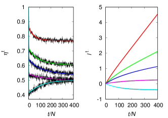
Figure 1: Time evolution of the mean fraction of lone agents $\eta^{t}$ (left panel) and mean loneliness per agent $l^{t}$ (right panel) for a population of size $N=50$ and mean number of contact attempts (from top to bottom) $q=0.1,0.3,0.5,1$ and $3$. The other parameters are $r=0.25$, $s=1$ and $\beta=1$. The critical point occurs at $q_{c}=0.587$. The colored thick lines are the mean-field predictions and the black thin lines are the averages over $10^{2}$ independent agent-based simulations. The initial conditions are $N_{a}^{0}=N$ and $L_{k}^{0}=0,k=1,\ldots,N$ so that $\eta^{0}=1$ and $l^{0}=0$.

In figure 1, we show the time evolution of $\eta^{t}$ and $l^{t}$ for the simulation of the agent-based model as well as for the mean-field approximation. The agreement between them is so remarkable that we have averaged those quantities over only 100 independent simulations in order to make the differences noticeable, though with no success in the case of the mean loneliness degree $l^{t}$. This agreement seems rather puzzling at first sight because the mean-field approximation exhibits a phase transition between the healthy and burnout regimes that cannot be observed in the ‘finite’ agent-based system of our simulations. In fact, the signatures of the phase transition, viz., the discontinuity of the derivative of the asymptotic value of $\eta^{t}$ with respect to $q$ and the divergence of the asymptotic value of $l^{t}$ at $q=q_{c}$, appear in the ‘thermodynamic’ limit only. As just hinted, the thermodynamic limit in our model is the time asymptotic limit $t\to\infty$ and since we cannot run infinitely long simulations we will never see those signatures in our simulation results. In figure 2, we illustrate this point by showing $\eta^{t}$ and $l^{t}$ evaluated at times $t=10^{3},10^{4}$ and $10^{5}$. These results indicate that the mean-field fixed points describe very accurately the asymptotic time behavior of the agent-based model.

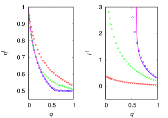
Figure 2: Mean fraction of lone agents $\eta^{t}$ (left panel) and mean loneliness per agent $l^{t}$ (right panel) evaluated at $t=10^{3}$ ($\triangledown$), $t=10^{4}$ ($\triangle$) and $t=10^{5}$ ($\circ$) as functions of the mean number of contact attempts $q$. The symbols represent the averages over $10^{4}$ independent agent-based simulations. The solid lines are the mean-field predictions for the limit $t\to\infty$. The critical point occurs at $q_{c}=0.587$. The other parameters are $N=50$, $r=0.25$, $s=1$ and $\beta=1$.

In figure 3, we show that the excellent agreement between the simulation and the mean-field results holds for other values of the model parameters too. As pointed out before, the discrepancies observed near the critical region are most likely due to the fact that we evaluate the time-asymptotic quantities at the finite time $t=10^{5}$. In particular, this figure highlights the curious finding that the rate of decrement of the loneliness degree due socialization $s$ has no influence on the number of lone agents in the burnout regime. The limit $q\to\infty$ guarantees that a lone agent will always find a conversation partner if there is one available. In this case, the mean-field approximation yields $\eta_{h}^{*}=s/(1+s)$ and $l^{*}=(1/2\beta)\ln\left[(r/s)/(1-r/s)\right]$ if $r/s<1$, and $\eta_{b}^{*}=r/(1+r)$ and $l^{*}\to\infty$ if $r/s\geq 1$.

Since the mean-field approximation describes the simulation results so well, it is instructive to look into its predictions near the critical point $q_{c}$ for $r/s<1$. In the healthy regime ($q>q_{c}$) we find

$$l^{*}\approx\frac{1}{2\beta}\ln(q-q_{c})$$ (24)

and $\eta^{*}_{h}=s/(1+s)$, whereas in the burnout regime ($q<q_{c}$) we find

$$\eta^{*}_{b}\approx\frac{s}{1+s}+\mathcal{A}(1-\frac{q}{q_{c}}),$$ (25)

where

$$\mathcal{A}=-\ln(1-r/s)\frac{s(s-r)(1-1/N)}{q_{c}s(s-r)+r(1+s)^{2}(1-1/N)}>0.$$ (26)

Hence, if we define the order parameter of the phase transition as $\rho=\eta_{b}^{*}-\eta_{h}^{*}$ then $\rho\sim(q_{c}-q)$ as we approach the critical point from the burnout regime.

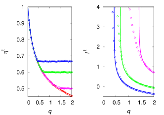
Figure 3: Mean fraction of lone agents $\eta^{t}$ (left panel) and asymptotic mean loneliness per agent $l^{t}$ (right panel) evaluated at $t=10^{5}$ as functions of the mean number of contact attempts $q$ for (left panel from top to bottom) $s=2,1.5,1$ and $0.5$. The symbols represent the averages over $10^{4}$ independent agent-based simulations and the solid lines are the mean-field predictions for the limit $t\to\infty$. The other parameters are $N=50$, $r=0.5$ and $\beta=1$. The data for $s=0.5$ is not shown in the right panel because $l^{*}$ diverges in the mean-field approximation and the simulations yield results that are well above the range of the y-axis.

At this stage, it is convenient to consider a more microscopic perspective of the community dynamics. We begin by pointing out that, since the $N$ agents are identical regarding the behavioral rules, the mean proportion of time that, say, agent $k$ spends alone equals the mean fraction of lone agents in the population for large $t$. Our simulations indicate that this equality holds true only when those quantities are averaged over many independent simulations, hence the adjective ‘mean’ in the above statement.

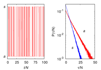
Figure 4: Sequence of flips between the conditions alone (a) and socializing (s) for a single agent in a single run (left panel) and probability distributions of the lengths of time $\tau$ that the agent spends in states a and s as indicated (right panel). The parameters are $N=50$, $r=0.1$, $s=2$ and $\beta=1$. The exponential probability distributions with means $\langle\tau_{\textsl{a}}\rangle/N=10$ and $\langle\tau_{\textsl{s}}\rangle/N=5$ were obtained using $10^{4}$ independent runs.

The left panel of figure 4 shows the flips between the alone (a) and the socializing (s) states experienced by a particular agent during a single run. The quantities of interest here are the lengths of the periods the agent spends alone $\tau_{\textsl{a}}$ and socializing $\tau_{\textsl{s}}$, whose probability distributions are shown in the right panel of the figure. Since those distributions are observed to be exponential distributions for large $t$, knowledge of the means $\langle\tau_{\textsl{a}}\rangle$ and $\langle\tau_{\textsl{s}}\rangle$ suffice to describe the random quantities $\tau_{\textsl{a}}$ and $\tau_{\textsl{s}}$ in the time-asymptotic limit. The probability distribution of $\tau_{\textsl{s}}$ is clearly exponential since once a couple of agents start socializing the duration of their conversation does not depend on their previous histories: the conversation is interrupted when either of the two socializing agents chooses to terminate it, which happens with probability $2r/N$ [see equation (8)] so that $\langle\tau_{\textsl{s}}\rangle/N=1/2r$ Feller_68 . As expected, the simulation results perfectly agree with this prediction (data not shown) which, we emphasize, does not involve any approximation.

However, the waiting time $\tau_{\textsl{a}}$ for a particular lone agent to start a social interaction does depend on its previous experiences since the propensity to socialize depends on its loneliness degree which, in some sense, encapsulates the life history of the agent. For instance, if the agent has just terminated a long conversation it is likely to spend a long time alone before being tempted to socialize again. Nevertheless, our simulations indicate that the probability distribution of $\tau_{\textsl{a}}$ can be described exceedingly well by an exponential distribution. In figure 5 we show $\langle\tau_{\textsl{a}}\rangle/N$ as function of the conversation termination probability $r$ for fixed $q$. In this setting, the phase transition occurs at

$$r_{c}/s=1-\exp\left(-q\frac{s/(1+s)-1/N}{1-1/N}\right),$$ (27)

which corresponds to the condition $\Lambda=1$ in equation (21). Since $r_{c}\leq 1$ there is a value of $s$ above which there is no phase transition and the model exhibits the healthy regime only. For $q=1$, this happens for $s>2.06$. In contrast to $\langle\tau_{\textsl{s}}\rangle/N$, the different time-asymptotic regimes strongly impact the dependence of $\langle\tau_{\textsl{a}}\rangle/N$ on $r$, as seen in figure 5. This is expected because the probability of finding a conversation partner (and hence of ending the loneliness period) depends on the fraction of lone agents $\eta^{t}$ in the community, which, in turn, exhibits rather distinct functional forms in the healthy and burnout regimes, as illustrated in figure 3.

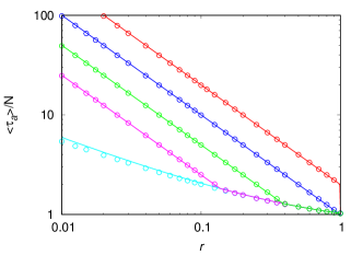
Figure 5: Mean time per agent that an agent spends alone $\langle\tau_{\textsl{a}}\rangle/N$ as function of the conversation termination probability $r$ for (top to bottom) $s=4,2,1,0.5$ and $0$. The symbols represent the averages over $10^{3}$ independent simulations with the waiting times $\tau_{\textsl{a}}$ recorded for $t\in[10^{5},10^{6}]$. The solid lines are the predictions of the ansatz (29). The other parameters are $N=50$, $q=1$ and $\beta=1$.

We observed that our simulation results for $\langle\tau_{\textsl{a}}\rangle/N$ can be described by a rather simple analytical expression (solid lines in figure 5) for which we have no explanation. The probability of the joint event that the lone agent $k$ is chosen for update at time $t$, decides to instigate a conversation and succeeds in finding another lone agent to interact with is

$$Q^{\prime}_{k}=\frac{p_{k}}{N}\left[1-\exp\left(-q\frac{\eta^{t}-1/N}{1-1/N}\right)\right],$$ (28)

which is the first term of the rhs of equation (II). In the limit of large $t$, we can replace $\eta^{t}$ by its mean-field estimate, namely, $\lim_{t\to\infty}\eta^{t}=\eta_{h}^{*}$ if $r\leq r_{c}$ and $\lim_{t\to\infty}\eta^{t}=\eta_{b}^{*}$ if $r>r_{c}$. We find that the ansatz

$$\langle\tau_{\textsl{a}}\rangle/N=1/(2NQ^{\prime}_{k})$$ (29)

offers a perfect fit for the simulation results, as shown in figure 5. In particular, using equation (16) for $r\leq r_{c}$ we obtain $NQ^{\prime}_{k}=r/s$ for large $t$ so that $\langle\tau_{\textsl{a}}\rangle/N=s/2r$. For $r>r_{c}$ we obtain $\langle\tau_{\textsl{a}}\rangle/N=\eta_{b}^{*}/[2r(1-\eta_{b}^{*})]$ where $\eta_{b}^{*}$ is the solution of equation (22). We note that the natural guess $\langle\tau_{\textsl{a}}\rangle/N=1/(NQ_{k})$ with $Q_{k}$ given by equation (II) yields qualitatively similar results but significantly underestimates the simulation results.

It is interesting that both waiting times decrease with increasing $r$. While this result is obvious for $\tau_{s}$, it is less apparent for $\tau_{a}$. In fact, it is the high availability of lone agents resulting from short conversations that produces the decrease of $\tau_{a}$. The reverse is also true: long socialization periods lead to long periods of loneliness because of the shortage of available partners. In addition, in the healthy regime, the lengths of the loneliness periods increase with the efficacy of social interactions in reducing loneliness, which is measured by the parameters $s$. This is expected, since the lesser the degree of loneliness of an agent, the less the probability that it will seek social contact. In the burnout regime, however, $\langle\tau_{\textsl{a}}\rangle/N$ does not depend on $s$ provided, of course, that $s$ does not become sufficiently large to allow the transition to the healthy regime.

V Conclusion

Since the main measure to curb the spread of SARS-CoV-2 is physical distancing, rather than social distancing, one may argue that internet-based and social media usage may mitigate the feelings of loneliness during the Covid-19 pandemic Smith2018 ; Banskota2020 . It is unclear, however, if use of technology to socialize remotely can significantly minimize those feelings Miller2018 . The key issue here is, of course, the quality of the social interactions. Our model takes this point into account through the parameter $s>0$ that measures the efficacy of the social interactions in decreasing feelings of loneliness. In fact, even if the number of contact attempts is unlimited (i.e., $q\to\infty$) and the community size is very large (i.e., $N\to\infty$), which is likely the case of social media, an agent can experience burnout in the case that $s<r$, where $r$ is the probability that the agent ends the social interaction. We recall that $s<a=1$ means that the rate of decrease of the feelings of loneliness when the agent is socializing is less than the rate of increase of those feelings when the agent is alone. It is clear then that $s$ can be used as a proxy for the quality of the social interactions. Therefore, our model describes the effects of the number of social contacts as well as of the quality of those contacts on loneliness. Both factors have been strongly affected by the physical distancing and quarantining measures widely implemented to prevent the spread of Covid-19.

We find that decrease of the number, quality or duration of social contacts lead the community to enter a regime of burnout in which the feelings of loneliness of the agents, measured by the variable $l^{t}$, diverge. This happens through a continuous phase transition that separates the healthy from the burnout regimes and that can be identified by the discontinuity of the derivative of the asymptotic fraction of lone agents with respect to the parameters of the model. Since the mean-field approximation reproduces the simulation results very well, equations (15), (16) and (17) offer a general formulation of the community dynamics where no assumptions are made on the influence of loneliness on the behavior of the agents, which is determined by the probabilities $p(l^{t})$ and $r(l^{t})$, as well as on the effect of that behavior on the feeling of loneliness, which is determined by the rates $M_{a}(l^{t})$ and $M_{s}(l^{t})$. In that sense, the community dynamics will exhibit a burnout regime provided that $\lim_{l^{t}\to\infty}r(l^{t})/p(l^{t})$ is nonzero. The appearance of this regime in our model illustrates neatly the side effects of the measures employed to curb the transmission of Covid-19 on the population mental health.

- (1) N. Leigh-Hunt, D. Bagguley, K. Bash, V. Turner, S. Turnbull, N. Valtorta, W. Caan, An overview of systematic reviews on the public health consequences of social isolation and loneliness, Public Health 152 (2017) 157–171, https://doi.org/10.1016/j.puhe.2017.07.035.
- (2) F.B. Alberti, A Biography of Loneliness: The History of an Emotion, Oxford University Press, New York, 2019.
- (3) P. Courtet, E. Olié, C. Debien, G. Vaiva, Keep socially (but not physically) connected and carry on: Preventing suicide in the age of COVID-19, J. Clin. Psychiatry 81 (3) (2020) 20com13370, https://doi.org/10.4088/JCP.20com13370.
- (4) Age UK, Jo Cox Commission Final Report (2017), https:// www.ageuk.org.uk/ globalassets/ age-uk/ documents/ reports-and-publications/ reports-and-briefings/ active-communities/ rb_dec17_jocox_commission_finalreport.pdf
- (5) E.D. Miller, Loneliness in the Era of COVID-19, Front. Psychol. 11 (2020) 2219, https://doi.org/10.3389/fpsyg.2020.02219
- (6) S. Galea, R.M. Merchant, N. Lurie, The mental health consequences of COVID-19 and physical distancing: the need for prevention and early intervention, JAMA Int. Med. 180 (6) (2020) 817–818, https://doi.org/10.1001/jamainternmed.2020.1562.
- (7) L.Y. Saltzman, C.H. Hansel, P.S. Bordnick, Loneliness, isolation, and social support factors in post-COVID-19 mental health, Psychol. Trauma 12 (S1) (2020) S55–S57, https://doi.org/10.1037/tra0000703.
- (8) N. Bellomo, R. Bingham, M.A.J. Chaplain, G. Dosi, G. Forni, D. A. Knopoff, J. Lowengrub, R. Twarock, M.E. Virgillito, A multiscale model of virus pandemic: Heterogeneous interactive entities in a globally connected world, Math. Models Methods Appl. Sci. 30 (8) (2020) 1591–1651, https://doi.org/10.1142/S0218202520500323.
- (9) A.M. Isen, K.A. Daubman, G.P. Nowicki, Positive affect facilitates creative problem solving, J. Pers. Soc. Psychol. 52 (6) (1987) 1122–1131, https://doi.org/10.1037/0022-3514.52.6.1122.
- (10) A. Oswald, E. Proto, D. Sgroi, Happiness and Productivity, J. Labor Econ. 33 (4) (2015) 789–822, https://doi.org/10.1086/681096.
- (11) M. Nicola, Z. Alsafi, C. Sohrabi, A. Kerwan, A. Al-Jabir, C. Iosifidis, M. Agha, R. Agha, The socio-economic implications of the coronavirus pandemic (COVID-19): A review, Int. J. Surg. 78 (2020) 185–193, https://doi.org/10.1016/j.ijsu.2020.04.018.
- (12) D.L. Phillips, Social participation and happiness, Am. J. Sociol. 72 (5) (1967) 479–488, https://doi.org/10.1086/224378.
- (13) C.W. McIntyre, D. Watson, L.A. Clark, S.A. Cross, The effect of induced social interaction on positive and negative affect, Bull. Psychon. Soc. 29 (1) (1991) 67–70, https://doi.org/10.3758/BF03334773
- (14) J.T. Cacioppo, L.C. Hawkley, Perceived Social Isolation and Cognition, Trends Cogn. Sci. 13 (10) (2009) 447–454, https://doi.org/10.1016/j.tics.2009.06.005.
- (15) B.G. Smith, S.B. Smith, D. Knighton, Social media dialogues in a crisis: A mixed-methods approach to identifying publics on social media, Public Relat. Rev. 44 (4) (2018) 562–573, https://doi.org/10.1016/j.pubrev.2018.07.005.
- (16) S. Banskota, M. Healy, E.M. Goldberg, 15 smartphone apps for older adults to use while in isolation during the COVID-19 pandemic. Western J. Emergency Med. 21 (3) (2020) 514–525, https://doi.org/10.5811/westjem.2020.4.47372.
- (17) L. Liang, H. Ren, R. Cao, Y. Hu, Z. Qin, L. Chuanen, M. Songli, The effect of COVID-19 on youth mental health, Psychiatr. Q. 91 (2020) 841–852, https://doi.org/10.1007/s11126-020-09744-3.
- (18) E.D. Miller, Cyberloneliness: the curse of the cursor?, in O. Sagan, E.D. Miller (Eds.), Narratives of Loneliness: Multidisciplinary Perspectives from the 21st Century, Routledge, London, pp. 56–65, 2018, https://doi.org/10.4324/9781315645582.
- (19) S.M. Moorman, Dyadic perspectives on marital quality and loneliness in later life, J. Soc. Personal Relat. 33 (5) (2016) 600–618, https://doi.org/10.1177/0265407515584504.
- (20) P. Hardy, L.S. Marcolino, J.F. Fontanari, The paradox of productivity during quarantine: an agent-based simulation, Eur. Phys. J. B 94 (1) (2021) 40, https://doi.org/10.1140/epjb/s10051-020-00016-4.
- (21) K. Huang, Statistical Mechanics, John Willey & Sons, New York, 1963.
- (22) W. Feller, An Introduction to Probability Theory and Its Applications, Vol. 1, Third Edition, Wiley, New York, 1968.