Anisotropic Heisenberg model for the mixed spin-3/2 and spin-1/2 under random crystal field

Abstract

Thermodynamic properties of the mixed spin-3/2 and spin-1/2 Heisenberg model are examined within the Oguchi approximation in the presence of a random crystal-field (RCF). The RCF is either introduced with probability $p$ or turned off with probability $1-p$ randomly. The thermal variations of the global magnetization and free energy of the system are investigated to construct the phase diagrams for the classical, quantum and anisotropic cases. Different results revealed that no qualitative changes exist between them. Quantum effects are found to be present and abundant in the quantum model in the negative $D$-range. This phenomenon has a strong decreasing effect on the critical temperature which becomes much lower than in the classical case. In the presence of an external field, it was observed that coercivity and remanence decrease in a wide range of the absolute temperature.

Key words: exchange anisotropy, Heisenberg model, Oguchi approximation, mixed spin, crystal field

Abstract

Òåðìîäèíàìiчíi âëàñòèâîñòi çìiøàíî¿ ñïií-3/2 òà ñïií-1/2 ìîäåëi Ãàéçåíáåðãà äîñëiäæóєòüñÿ â íàáëèæåííi Îãóчi çà íàÿâíîñòi âèïàäêîâîãî êðèñòàëiчíîãî ïîëÿ (ÂÊÏ). ÂÊÏ àáî ââîäèòüñÿ ç iìîâiðíiñòþ $p$, àáî âèìèêàєòüñÿ ç éìîâiðíiñòþ $1-p$ âèïàäêîâî. Äîñëiäæóþòüñÿ òåïëîâi êîëèâàííÿ ãëîáàëüíîãî íàìàãíiчóâàííÿ òà âiëüíà åíåðãiÿ ñèñòåìè äëÿ òîãî, ùîá ïîáóäóâàòè ôàçîâi äiàãðàìè äëÿ êëàñèчíèõ, êâàíòîâèõ òà àíiçîòðîïíèõ âèïàäêiâ. Îòðèìàíi ðiçíi ðåçóëüòàòè ïîêàçóþòü, ùî ìiæ íèìè íå iñíóє ÿêiñíèõ çìií. Âñòàíîâëåíî ïðèñóòíiñòü êâàíòîâèõ åôåêòiâ ó êâàíòîâié ìîäåëi â íåãàòèâíîìó $D$-äiàïàçîíi. Öåé ôåíîìåí âèÿâëÿє ñèëüíèé çìåíøóâàëüíèé âïëèâ íà êðèòèчíó òåìïåðàòóðó, ÿêà ñòàє íàáàãàòî íèæчîþ, íiæ ó êëàñèчíîìó âèïàäêó. Ïðè íàÿâíîñòi çîâíiøíüîãî ïîëÿ, ñïîñòåðiãàëîñü, ùî êîåðöèòèâíiñòü i çàëèøêîâà íàìàãíiчåíiñòü çìåíøóþòüñÿ â øèðîêîìó äiàïàçîíi àáñîëþòíèõ òåìïåðàòóð.

Ключовi слова: îáìiííà àíiçîòðîïiÿ, ìîäåëü Ãàéçåíáåðãà, íàáëèæåííÿ Îãóчi, çìiøàíèé ñïií, êðèñòàëiчíå ïîëå

1 Introduction

In the classical spin models, e.g., Ising model (IM), the spins can only lie along one chosen axis which is often taken to be the $z$-axis. These systems may be relatively easy to deal with when compared with the quantum spin models, i.e., Heisenberg model (HM), because the spins now have freedom to orient themselves in any three-dimensional space. This, of course, leads to an uncertainty since the spin operators, i.e., the components of a spin, do not commute with each other. Therefore, it is usually impossible to obtain an analytical solution. Their solutions often require some possible approximations which may provide qualitative pictures but mostly presents some shortcomings.

The Oguchi approximation (OA) is such an approximation which is used to solve the HMs. The spin-1/2 anistropic HM was studied with Dzyaloshinsky-Moriya interaction [1]. The effects of the second-nearest-neighbor exchange interactions on the magnetization, internal energy, heat capacity, entropy and free energy were examined [2]. The phase diagrams of the mixed spin-1 and spin-1/2 under the influence of both exchange and single-ion anisotropies were taken into consideration [3]. This model was also extended to the studies of compensation temperature [4] and magnetic susceptibility [5]. The mixed spin-2 and spin-1/2 HM was studied under the influence of exchange anisotropy and crystal field by using the OA on the square [6] and simple cubic lattices [7]. A similar study was also performed on the ferromagnetic mixed spin-3/2 and spin-1/2 model for the HM in terms of the OA [8].

In addition to the HM in the OA approximation, there are some other works which use some other techniques, considering various aspects in the IM. The first technique is the effective field theory (EFT) which was considered in the calculation of magnetizations and phase diagrams [9], the critical properties in a transverse field [10], magnetic properties in a longitudinal magnetic field [11], the magnetic and hysteresis behaviors for a bilayer model [12], bimodal random-crystal field distribution effects [13], for a ferromagnetic or antiferromagnetic bilayer system with transverse field [14, 15], in a random field [16], and for a trimodal random-field distribution [17]. Some of the works with a diluted model were also examined in the EFT in a random field [18], with coordination numbers 3 and 4 [19], in a longitudinal random field [20], for transverse Ising model [21, 22] and for the study of the magnetic properties[23]. In addition to the EFT studies, the Monte Carlo algorithm [24], the exact recursion relations (ERR) were used on the Bethe lattice (BL) [25], by establishing a mapping correspondence with the eight-vertex model [26], an exact star-triangle mapping transformation [27], the ERR’s on a two-fold Cayley tree [28], on the Union Jack lattice by means of a mapping correspondence with the eight-vertex model [29], on a rope ladder it was examined by combining two exact analytical methods, i.e., decoration-iteration mapping transformation and standard transfer-matrix method [30], within the mean-field approximation [31] and with the use of the ERR’s on the BL [32], on a two-layer BL [33] and $\pm J$ model [34].

In this work, we extend the study of the mixed-spin 3/2 and 1/2 HM in the OA [8] with the inclusion of the RCF and examine its phase diagrams by studying the thermal variations of total and relative magnetizations as well as the free energy. The hysteresis cycles behavior is also analysed at different temperatures.

The rest of the work is arranged as follows: The next section is devoted to the formulation of Heisenberg model in the Oguchi approximation for the mixed spin-3/2 and 1/2 system under the effect of the RCF. The third section consists of illustrations and possible discussions and comparisons. The final section is devoted to a brief summary and conclusion.

2 The formulation of the HM in the OA for the mixed-spin 3/2 and 1/2 model

A lattice with coordination number $q$ is considered. It is devided into two equivalent sublattices A and B with spins 1/2 and 3/2, respectively. The usual Heisenberg Hamiltonian is considered. It includes the nearest-neighbor (NN) bilinear interaction parameter $J$, the random crystal field $D_{i}$ active only at spin-3/2 sites and the external magnetic field $h$. Its expression follows:

$$\hat{\mathcal{H}}= - J\sum\limits_{\langle ij\rangle}\left[(1-\Delta)(\hat{S}_{i,3/2}^{x}\hat{S}_{j,1/2}^{x}+\hat{S}_{i,3/2}^{y}\hat{S}_{j,1/2}^{y})+\hat{S}_{i,3/2}^{z}\hat{S}_{j,1/2}^{z}\right]$$ (2.1)

$$- \sum\limits_{i}D_{i}{\left(\hat{S}_{i,3/2}^{z}\right)^{2}}-h\left(\sum_{i}S_{i,3/2}^{z}+\sum_{j}S_{j,1/2}^{z}\right),$$

where $S_{i,3/2}^{\nu}$ and $S_{j,1/2}^{\nu}$ with $\nu=x,y,z$ are the components of spin operators for spin-3/2 and spin-1/2 and $\Delta$ is the exchange anisotropy parameter with $0\leqslant\Delta\leqslant 1$. The values of $\Delta$ changes it into the IM Hamiltonian when it is set to one, into the HM Hamiltonian when it is equal to zero and into the anisotropic model (AM) Hamiltonian when $0<\Delta<1$.

To solve the model, some approximations are necessary. In the OA, the effective Oguchi Hamiltonian for a pair of 3/2 and 1/2 spins is given as

$$\hat{\mathcal{H}}_{ij}= - J\left[(1-\Delta)(\hat{S}_{i,3/2}^{x}\hat{S}_{j,1/2}^{x}+\hat{S}_{i,3/2}^{y}\hat{S}_{j,1/2}^{y})+\hat{S}_{i,3/2}^{z}\hat{S}_{j,1/2}^{z}\right]$$ (2.2)

$$- D_{i}{\left(\hat{S}_{i,3/2}^{z}\right)^{2}}-h_{i}\hat{S}_{i,3/2}^{z}-h_{j}\hat{S}_{j,1/2}^{z}\,,$$

where the mean-field terms are given as

$$h_{i}=h+(q-1)JM_{1/2}\,,$$

$$h_{j}=h+(q-1)JM_{3/2}\,,$$ (2.3)

with $M_{3/2}=\langle\hat{S}_{i,3/2}^{z}\rangle$ and $M_{1/2}=\langle\hat{S}_{j,1/2}^{z}\rangle$ being the magnetizations of the sublattices with spin-3/2 and spin-1/2, $q$ is the number of NN’s, and $\langle...\rangle$ corresponds to thermal averages.

One has to solve the eigenvalue equation

$$\hat{\mathcal{H}}_{ij}\mid n\rangle=H_{n}\mid n\rangle,\qquad n=1,2,\ldots,8$$ (2.4)

in order to get our required thermodynamic functions. Here, the $\mid n\rangle$’s are the eigenvectors and $H_{n}$ are the eigenvalues. The direct products of the possible vectors $|s_{3/2},m_{3/2}\rangle_{i}$ for spin-3/2 and $|s_{1/2},m_{1/2}\rangle_{j}$ for spin-1/2 should be calculated. The direct product, i.e., $|s_{3/2},m_{3/2}\rangle_{i}\otimes|s_{1/2},m_{1/2}\rangle_{j}$, gives us eight possible base vectors as

$$|I\rangle=|3/2,3/2\rangle_{i}|1/2,1/2\rangle_{j}\,,\hskip 31.2982pt|II\rangle=|3/2,3/2\rangle_{i}|1/2,-1/2\rangle_{j}\,,$$

$$|III\rangle=|3/2,-3/2\rangle_{i}|1/2,1/2\rangle_{j}\,,\hskip 12.80365pt|IV\rangle=|3/2,-3/2\rangle_{i}|1/2,-1/2\rangle_{j}\,,$$

$$|V\rangle=|3/2,-1/2\rangle_{i}|1/2,1/2\rangle_{j}\,,\hskip 19.91684pt|VI\rangle=|3/2,-1/2\rangle_{i}|1/2,-1/2\rangle_{j}\,,$$

$$|VII\rangle=|3/2,1/2\rangle_{i}|1/2,1/2\rangle_{j}\,,\hskip 17.07182pt|VIII\rangle=|3/2,1/2\rangle_{i}|1/2,-1/2\rangle_{j}.$$ (2.5)

These eigenvectors are used to obtain the matrix form of $\hat{\mathcal{H}}_{ij}$ which is $8\times 8$ matrix whose elements are obtained from $H_{ij}=\langle i|\hat{\mathcal{H}}_{ij}|j\rangle$ with $i,j=I,II,...,VIII$ and it is found as:

$$H_{ij}=\left(\begin{array}[]{cccccccc}H_{11}&0&0&0&0&0&0&0\\ 0&H_{22}&-\sqrt{3}*t&0&0&0&0&0\\ 0&-\sqrt{3}*t&H_{33}&0&0&0&0&0\\ 0&0&0&H_{44}&2*t&0&0&0\\ 0&0&0&2*t&H_{55}&0&0&0\\ 0&0&0&0&0&H_{66}&-\sqrt{3}*t&0\\ 0&0&0&0&0&-\sqrt{3}*t&H_{77}&0\\ 0&0&0&0&0&0&0&H_{88}\end{array}\right)\,,$$ (2.6)

where the diagonal matrix elements are found as

$$H_{11}=-\frac{3J}{4}-\frac{9D_{i}}{4}-\frac{3h_{i}}{2}-\frac{h_{j}}{2},\hskip 14.22636ptH_{22}=\frac{3J}{4}-\frac{9D_{i}}{4}-\frac{3h_{i}}{2}+\frac{h_{j}}{2},$$

$$H_{33}=-\frac{J}{4}-\frac{D_{i}}{4}-\frac{h_{i}}{2}-\frac{h_{j}}{2},\quad\hskip 18.49411ptH_{44}=\frac{J}{4}-\frac{D_{i}}{4}-\frac{h_{i}}{2}+\frac{h_{j}}{2},$$

$$H_{55}=\frac{J}{4}-\frac{D_{i}}{4}-\frac{h_{i}}{2}-\frac{h_{j}}{2},\quad\hskip 24.18501ptH_{66}=-\frac{J}{4}-\frac{D_{i}}{4}-\frac{h_{i}}{2}+\frac{h_{j}}{2},$$

$$H_{77}=\frac{3J}{4}-\frac{9D_{i}}{4}-\frac{3h_{i}}{2}-\frac{h_{j}}{2},\hskip 17.07182ptH_{88}=-\frac{3J}{4}-\frac{9D_{i}}{4}-\frac{3h_{i}}{2}-\frac{h_{j}}{2},$$ (2.7)

with $t=-{\frac{J}{2}(1-\Delta_{0})}$. The eigenvalues of this matrix $H_{ij}$ are calculated as:

$$\lambda_{1}=H_{11},$$

$$\lambda_{2}=-{{\sqrt{12t^{2}+H_{66}^{2}-2H_{66}H_{77}+H_{77}^{2}}-\,H_{66}-H_{77}}\over{2}},$$

$$\lambda_{3}={{\sqrt{12t^{2}+H_{66}^{2}-2H_{66}H_{77}+H_{77}^{2}}+\,H_{66}+H_{77}}\over{2}},$$

$$\lambda_{4}=-{{\sqrt{16t^{2}+H_{44}^{2}-2H_{44}H_{55}+H_{55}^{2}}-\,H_{44}-H_{55}}\over{2}},$$

$$\lambda_{5}={{\sqrt{16t^{2}+H_{44}^{2}-2H_{44}H_{55}+H_{55}^{2}}+\,H_{44}+H_{55}}\over{2}},$$

$$\lambda_{6}=-{{\sqrt{12t^{2}+H_{22}^{2}-2H_{22}H_{33}+H_{33}^{2}}-\,H_{22}-H_{33}}\over{2}},$$

$$\lambda_{7}={{\sqrt{12t^{2}+H_{22}^{2}-2H_{22}H_{33}+H_{33}^{2}}+\,H_{22}+H_{33}}\over{2}},$$

$$\lambda_{8}=H_{88}.$$ (2.8)

After obtaining the eigenvalues, we are now ready to obtain the partition function which is the main ingredient of our calculation which is found from $Z=\mathrm{Tr}_{ij}[\exp(-\beta H_{ij})]$ and calculated as:

$$Z = \sum\limits_{n=1}^{8}\exp(-\beta\lambda_{n})$$

$$= \exp(-\beta H_{11})+\exp\left(-\beta H_{88}\right)$$

$$+ 2\exp\Big{[}-\beta(H_{22}+H_{33})\Big{]}\cosh\left(\frac{\beta\omega_{23}}{2}\right)$$

$$+ 2\exp\Big{[}-\beta(H_{44}+H_{55})\Big{]}\cosh\left(\frac{\beta\omega_{45}}{2}\right)$$

$$+ 2\exp\Big{[}-\beta(H_{66}+H_{77})\Big{]}\cosh\left(\frac{\beta\omega_{67}}{2}\right),$$

where $\beta=\frac{1}{k_{\text{B}}T}$, $\omega_{23}=\lambda_{3}-\lambda_{2}$, $\omega_{45}=\lambda_{5}-\lambda_{4}$, $\omega_{67}=\lambda_{7}-\lambda_{6}$ and $k_{\text{B}}$ is the Boltzmann constant.

The magnetizations for spin-3/2 and spin-1/2 are calculated by using the definitions

$$M_{3/2}=\frac{1}{\beta Z}\frac{\partial Z}{\partial h_{i}}$$ (2.9)

and

$$M_{1/2}=\frac{1}{\beta Z}\frac{\partial Z}{\partial h_{j}}.$$ (2.10)

In addition, the average magnetization can be defined as

$$M_{T}=(M_{3/2}+M_{1/2})/2.$$ (2.11)

Finally, the free energy of the model can be obtained by using

$$F=-(1/\beta)\ln Z+J(q-1)M_{3/2}M_{1/2}.$$ (2.12)

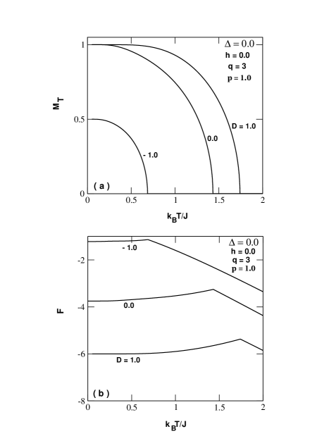
Figure 1: Temperature dependence of global magnetization (panel a) and the free energy (panel b) of the system when $\Delta=0.0$, $q=3$, $h=0.0$ and $p=1.0$ for selected values of the crystal-field.

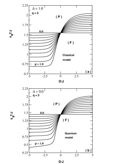
Figure 2: Phase diagrams of the system in the $(D/J,k_{\text{B}}T/J)$ plane for selected values of the probability $p$ between 0 and 1 with an increment of 0.1 for $\Delta=1.0$ (panel a) and $\Delta=0.0$ (panel b) and $q=3$.

So far all the equations are obtained for the mixed spin-3/2 and 1/2 HM in the OA. In order to implement the RCF that is given in the bimodal form which turns the crystal field on with probability $p$ and turns it off with $1-p$

$$P(D_{i})=p\delta(D_{i}-D)+(1-p)\delta(D_{i})$$

must be combined with the final forms of magnetizations. Thus, the magnetizations with RCF effects can be obtained from

$$m_{3/2}=\int\frac{1}{\beta Z}\Big{[}\frac{\partial{Z}}{\partial{h_{i}}}\Big{]}P(D_{i})\mathrm{d}D_{i}$$ (2.13)

and

$$m_{1/2}=\int\frac{1}{\beta Z}\Big{[}\frac{\partial{Z}}{\partial{h_{j}}}\Big{]}P(D_{i})\mathrm{d}D_{i}.$$ (2.14)

Lastly, the free energy with RCF is also given as

$$f = -\frac{1}{\beta}\int\ln ZP(D_{i})\mathrm{d}D_{i}.$$ (2.15)

In the next section, we are going to illustrate our findings in terms of possible phase diagrams, thermal variations of magnetizations and magnetic hysteresis loops.

3 The phase diagrams

We start this section by analyzing the thermal behavior of the order parameters which are reduced in the model to the global magnetization of the system. This is depicted in figure 1a for the coordination number $q=3$. As usually observed, the total magnetization starts from its saturation values and, as thermal fluctuations grow in the system, it continuously decreases and finally vanishes at the critical temperature $T_{c}$. As it can be observed, the displayed curves correspond to selected values of the crystal-field $D$. It immediately appears that when $D$ increases, a coexistence point between thermodynamic phases (1/2, 1/2) and (3/2, 1/2) may appear because there exist two different saturation values of the global magnetization. The transition which is previously observed when $M$ vanishes is of the second-order and $T_{c}$ increases when the value of $D$ is raised. This means that $D$ produces some stabilizing effect on the ordered ferrimagnetic phase whose volume also increases. In figure 1b, the free energy is illustrated and shows two different behaviors separated by a peak which is associated with the critical temperature $T_{c}$. One can see the first region where it slowly increases. This increase becomes pronounced when $D$ gets larger values. In the second region, a very fast decay of the free energy is observed because the entropy term exceeds the internal energy leading to almost straight lines. Similar results were reported in [35] which dealt with thermodynamic properties of a spin-1/2 Heisenberg ferromagnetic system within the same Oguchi’s approximation. Therein, the internal energy $U$ is monitored and exhibited, as the entropy, a constant for $T>T_{c}$.

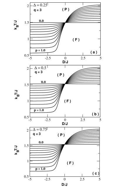
Figure 3: Phase diagrams of the system in the $(D/J,k_{\text{B}}T/J)$ plane for selected values of the probability $p$ between 0 and 1 with an increment of 0.1 for $\Delta=0.25$ (panel a); $\Delta=0.5$ (panel b) and $\Delta=0.75$ (panel c) and $q=3$.

For varying values of the crystal-field interaction parameter $D$ and probability distribution $p$, one is able to devise a phase diagram for the model in the ($D/J,k_{\text{B}}T/J$) plane. This is done in figures 2a and b for the classical version ($\Delta=1$) and the quantum version ($\Delta=0$). Both panels show similar qualitative trends. Some interesting features emerge. In particular, it is observed that the critical temperature $T_{c}$ becomes insensitive to the value of the crystal-field parameter when this value becomes relatively high at any value of the probability $p$. This behavior is observed in several previous works. In fact, [36] that dealt with exact calculations on the mixed spin-1/2 and spin-S model on the square lattice reported similar trends. For large and positive/negative values of $D$, thermodynamic phases (3/2,1/2)/(1/2,1/2) should prevail in the system. It could be observed in the case that the difference between the asymptotic values of the critical temperature $T_{c}$ is a decreasing function of the parameter $p$ that vanishes at $p=0$. Our calculations for these asymptotic values lead to the following results. In the classical model, for $p=0;\,0.5;\,1$ and $D\rightarrow-\infty/+\infty$, we get respectively $k_{\text{B}}T/J=1.548/1.548$; $k_{\text{B}}T/J=1.200/1.810$; $k_{\text{B}}T/J=0.691/2.051$. In the quantum model case, for $p=0;\,0.5;\,1$ and $D\rightarrow-\infty/+\infty$, one respectively obtains $k_{\text{B}}T/J=1.446/1.446$; $k_{\text{B}}T/J=1.075/1.769$; $k_{\text{B}}T/J=0.346/2.037$. It emerges that the change of the gap when $p$ runs from $0$ to $1$ becomes considerably larger in the case of negative values of $D$ than for positive values in both models. When comparing the results displayed in both panels, it evidently appears that the quantitative change of the critical temperature $T_{c}$ could be clearly seen in the negative $D$-range considered whereas only similar qualitative trends are observed beyond. As an example, for $p=1$, the critical temperature $T_{c}$ for the quantum model is about half of that of the classical model, which means that quantum effects play a key role in the magnetic properties of the quantum system for negative values of the parameter $D$ which are associated with low values of $T_{c}$. For this value of $p$, quantum effects on the critical temperature are negligible at high values of $D$ which induce $T_{c}$.

After studying the phase diagrams for the two extreme cases, $\Delta=0;1$, the anisotropic case $\Delta\neq 0;1$ needs to be somewhat clarified. Results concerning this intermediate case are illustrated in figure 3. As it can be seen from different panels, the anisotropic case shows the same qualitative behavior of phase boundaries with the extreme quantum case. At fixed values of $p$, one sees that $T_{c}$ is an increasing function of $\Delta$. The value corresponding to the saturation of $T_{c}$ in the negative $D$-range also increases when the value of $\Delta$ is raised.

In figure 4, we show another way to present the results reported in figure 2. We display phase diagrams in the ($p,k_{\text{B}}T/J$) plane for selected values of the crystal-field for the classical and quantum models. For $\Delta=0$, one gets a straight and horizontal second-order transition line. For increasing values of $D$, we get increasing values of $T_{c}$ whereas for decreasing negative values, the contrary holds. Throughout the previous figures, our numerical calculations only show second-order transition. As it is shown in the following, one can get first-order transitions in the model at a relatively high value of the coordination parameter $q$ as well as in the presence of an external magnetic field constraint.

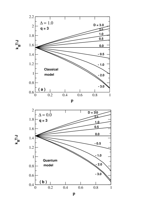
Figure 4: Phase diagrams of the system in the $(p,k_{\text{B}}T/J)$ plane for selected values of $D$ for $\Delta=1.0$ (panel a); $\Delta=0.0$ (panel b) and $q=3$.

In fact, in figure 5, we present a set of phase diagrams for the quantum model in the $(D/J,k_{\text{B}}TJ)$ plane for selected values of the probability $p$ and coordination number $q=6$. The case $q=6$ should correspond to the simple cubic lattice case. The number of nearest-neighbor interactions is then increased. For $p=0$, one gets the same straight line separating the ferrimagnetic and the disordered paramagnetic phases as in figures 2,3. For $p\geqslant 0$, the results indicate the appearance of first-order transitions that are localized by jumps in the global magnetization of the system. This is observed in the very low-temperature range and for a $D/J$ value around $-1.4$. Thus, the results for $(p=1;\Delta=0)$ (panel d) correspond to the results reported in figure 3 of [8]. Let us remind the reader that the introduction of the probability distribution on the crystal-field is the only difference between our model and that of [8]. A careful observation of the onset of the first order transition when the parameter $p$ varies shows that the value of $D$ associated with this onset decreases with $p$. Our calculations show that the first order transition lines observed in the panels terminate at end-points. Hence, the critical values associated with $p=0.5,\,0.8,\,1$ are respectively: $(D/J=-1.45,k_{\text{B}}T/J=0.035)$, $(D/J=-1.44,k_{\text{B}}T/J=0.042)$, $(D/J=-1.424,k_{\text{B}}T/J=0.071)$.

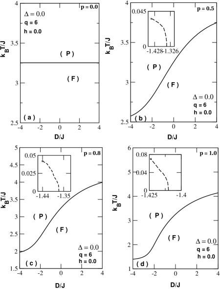
Figure 5: Phase diagrams of the system in the $(D/J,k_{\text{B}}T/J)$ plane for $p=0.0$ (panel a); $p=0.5$ (panel b); $p=0.8$ (panel c); $p=1.0$ (panel d) and $q=6$. A first-order transition phenomenon is detected at low temperature for negative values of $D/J$.

In what follows, the influence of the applied magnetic field is examined on the quantum system. Figure 6a illustrates the change of the first-order transition temperature with the value of the crystal-field $D$. At a constant value $h=-0.5$, one sees that this temperature increases when the value of the crystal-field increases. The corresponding free energies in figure 6c show discontinuities at the transition temperatures. This insures that we are in fact in the presence of true first-order transitions rather than the jumps of the system from metastable states to stable (steady) states when thermal fluctuations are enhanced. Figure 6b illustrates how the first-order transition is affected when $h$ varies. It could be observed that no transition appears with positive values of the field $h$. All these observed behaviors result from the competition between different model parameters of the system when the temperature varies.

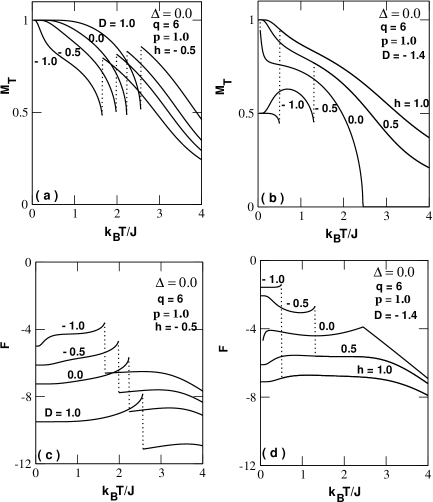
Figure 6: The behaviors of the magnetization ( panels a,b) and the free energy ( panels c,d) as functions of the temperature $T$. In panel a, the effect of the crystal-field on the first-order transition is illustrated whereas panel b shows how the values of h displace this transition.

Different panels of figure 7 show hysteresis phenomena and how the system disorders when the temperature is raised from zero. It also appears that the coercitive field $h_{c}$ and the remannent magnetization $m_{r}$ decrease with the temperature $T$ since at high temperature a critical hysteresis is obtained.

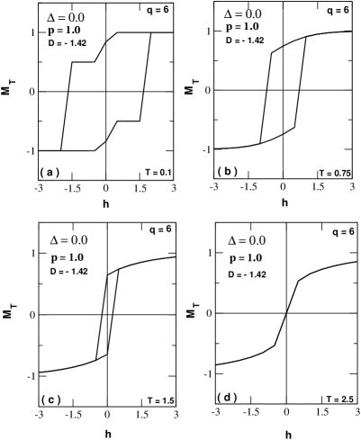
Figure 7: Typical hysteresis behavior of the system as a function of the applied field h for selected values of the temperature $T$.

Figure 8 gives detailed illustrations of that. Ou results for $h_{c}$ look similar to those displayed in [37, 38]. The remanent magnetization shows a narrow low-temperature region where it increases with $T$. Beyond this region, it behaves like the global magnetization and vanishes at critical temperatures corresponding to selected values of $p$. A similar behavior is also observed for the coercivity.

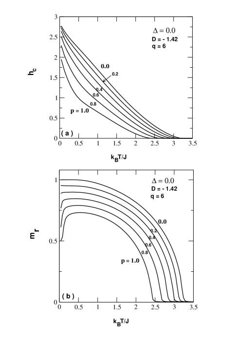
Figure 8: The coercive field $h_{c}$ (panel a) and the remanent magnetization (panel b) as functions of the temperature for selected values of the model parameters.

4 Brief summary and conclusion

In this work, the mixed spin-3/2 and spin-1/2 Heisenberg model was investigated by means of the Oguchi approximation which is a kind of a Mean Field treatment. The classical, quantum and anisotropic cases were analyzed in the presence of a random crystal-field which was set on the system with probability $p$ or turned off with probability $1-p$. Computed magnetizations in the quantum case showed the presence of second-order phase transitions for the coordination number $q=3$ in the absence of the external magnetic field $h$. The free energy $F$ was found to increase with thermal fluctuations in the ferrimagnetic phase whereas a decrease emerged at the onset of total disorder in the system. For $q=3$, several phase diagrams are plotted for varying values of the anisotropy $\Delta$ and probability $p$. It was observed that quantum effects are almost absent in the positive $D$-range whereas for relatively low and negative values of $D$ they appeared important, in particular in the quantum model for $p=1$. Our calculations did not show first-order transitions for $q=3$. Instead, for $q=6$, this phenomenon appeared at a very low temperature in the negative $D$-range even in the absence of the external field constraint. It was also revealed that for positive values of $h$, the first-order transition was absent whereas beyond, at least in the range of selected values of $h$ used in the computations, it appeared and the corresponding temperature decreases with the absolute value of $h$. The existence of first-order transition induced the presence of a hysteresis phenomenon in the quantum model. It was also shown that thermal fluctuations had a dramatic effect on the size of the hysteresis loop which decreases as the temperature increases and finally generates a critical hysteresis. Finally, we found that coercivity and remanence decrease with the temperature in a wide range of the temperature $T$.

Ukrainian 0

Àíiçîòðîïíà ìîäåëü Ãàéçåíáåðãà çìiøàíîãî òèïó ñïií-3/2 òà ñïií-1/2 ïiä äiєþ âèïàäêîâîãî êðèñòàëiчíîãî ïîëÿ

Ä. Ñàái Òàêó${}^{\textsf{\footnotesize{\mbox{?},\penalty 1000\mbox{?}}}}$, M. Êàðiìó${}^{\textsf{\footnotesize{\mbox{?},\penalty 1000\mbox{?}}}}$, Ô. Ãîíòiíôiíäå${}^{\textsf{\footnotesize{\mbox{?},\penalty 1000\mbox{?}}}}$, Å. Àëáàéðàê${}^{\textsf{\footnotesize{\mbox{?}}}}$

             
${}^{\textsf{\footnotesize 1}}$ Âèùà ïîëiòåõíiчíà øêîëà Àáîìåé-Êàëàâi (EPAC-UAC), ôàêóëüòåò ïðèðîäíèчèõ íàóê, Ðåñïóáëiêà Áåíií ${}^{\textsf{\footnotesize 2}}$ Íàöiîíàëüíà âèùà øêîëà åíåðãåòèêè i ïðîöåñiâ (ENSGEP), Àáîìåé, Ðåñïóáëiêà Áåíií ${}^{\textsf{\footnotesize 3}}$ Iíñòèòóò ìàòàìàòèчíèõ i ôiçèчíèõ íàóê (IMSP), Ðåñïóáëiêà Áåíií ${}^{\textsf{\footnotesize 4}}$ Óíiâåðñèòåò Àáîìåé-Êàëàâi, ôiçèчíèé ôàêóëüòåò, Ðåñïóáëiêà Áåíií ${}^{\textsf{\footnotesize 5}}$ Óíiâåðñèòåò Åðäæiєñ, ôiçèчíèé ôàêóëüòåò, 38039, Êàéñåði, Òóðåччèíà

References

-
[1]
Ricardo de Sousa J., Lacerda F., Fittipaldi I.P., Physica A, 1998, 258, 221–229,
doi:10.1016/S0378-4371(97)00537-2. - [2] Mert G., J. Magn. Magn. Mater., 2015, 394, 126–129, doi:10.1016/j.jmmm.2015.06.062.
- [3] Bobák A., Pokorný V., Dely J., Physica A, 2009, 388, 2157–2167, doi:10.1016/j.physa.2009.02.017.
- [4] Bobák A., Dely J., Žukovič M., Physica A, 2011, 390, 1953–1960, doi:10.1016/j.physa.2011.02.028.
- [5] Bobák A., Pokorny V., Dely J., J. Phys. Conf. Ser., 2010, 200, 022001, doi:10.1088/1742-6596/200/2/022001.
- [6] Albayrak E., J. Supercond. Novel Magn., 2017, 30 2555–2561, doi:10.1007/s10948-017-4079-4.
- [7] Albayrak E., Physica A, 2017, 486, 161–167, doi:10.1016/j.physa.2017.05.042.
-
[8]
Bobák A., Fecková Z., Žukovič M., J. Magn. Magn. Mater., 2011, 323, 813–818,
doi:10.1016/j.jmmm.2010.11.003. -
[9]
Kaneyoshi T., Jaščur M., Tomczak P., J. Phys: Condens. Matter, 1992, 4, L653–L658,
doi:10.1088/0953-8984/4/49/002. - [10] Kaneyoshi T., Physica A, 1995, 215, 378–386, doi:10.1016/0378-4371(94)00306-E.
-
[11]
Wei G.Z., Liang Y.Q., Zhang Q., Xin Z.H., J. Magn. Magn. Mater., 2004, 271, 246–253,
doi:10.1016/j.jmmm.2003.09.043. - [12] Essaoudi I., Bärner K., Ainane A., Saber M., Physica A, 2007, 385, 208–220, doi:10.1016/j.physa.2007.06.037.
- [13] Yigit A., Albayrak E., J. Magn. Magn. Mater., 2013, 329, 125–128, doi:10.1016/j.jmmm.2012.10.011.
- [14] Jiang W., Wei G.Z., Du A., J. Magn. Magn. Mater., 2002, 250, 49–56, doi:10.1016/S0304-8853(02)00351-7.
-
[15]
Htoutou K., Ainane A., Saber M., J. Magn. Magn. Mater., 2004, 269, 245–258,
doi:10.1016/j.jmmm.2003.07.002. -
[16]
Liang Y.Q., Wei G.Z., Zhang Q., Wei Q., Zang S.L., Chin. Phys., 2004, 13, 2147,
doi:10.1088/1009-1963/13/12/030. -
[17]
Liang Y.Q., Wei G.Z., Song G.L., Phys. Status Solidi B, 2004, 241, 1916, 1916–1922,
doi:10.1002/pssb.200301996. - [18] Kaneyoshi T., J. Magn. Magn. Mater., 1995, 151, 45–53, doi:10.1016/0304-8853(95)00403-3.
- [19] Bobák A., Jurčišin M., J. Magn. Magn. Mater., 1996, 163, 292–298, doi:10.1016/S0304-8853(96)00353-8.
- [20] Liang Y.Q., Wei G.Z., Song G.L., Phys. Status Solidi B, 2008, 245, 2586, doi:10.1002/pssb.200844136.
- [21] Benayad N., Dakhama A., Klümper A., Zittartz J., Z. Phys. B: Condens. Matter, 1996, 101, 623–630, doi:10.1007/s002570050255.
- [22] Jiang W., Wei G.Z., Xin Z.H., Physica A, 2001, 293, 455–464, doi:10.1016/S0378-4371(01)00008-5.
-
[23]
Bobák A., Horváth D., Phys. Status Solidi B, 1999, 213, 459,
doi:10.1002/(SICI)1521-3951(199906)213:2<459::AID-PSSB459>3.0.CO;2-0. - [24] Buendia G.M., Cardano R., Phys. Rev. B, 1999, 59, 6784, doi:10.1103/PhysRevB.59.6784.
- [25] Albayrak E., Alçı A., Physica A, 2005, 345, 48–60, doi:10.1016/j.physa.2004.04.134.
- [26] Strečka J., Čanová L., Condens. Matter Phys., 2006, 9, 179, doi:10.5488/CMP.9.1.179.
- [27] Jaščur M., Strečka J., Physica A, 2005, 358, 393, doi:10.1016/j.physa.2005.07.010.
- [28] Zhang X., Kong X.M., Physica A, 2006, 369, 589–598, doi:10.1016/j.physa.2006.02.014.
- [29] Strečka J., Phys. Status Solidi B, 2006, 243, 708, doi:10.1002/pssb.200642018.
- [30] Kiššova J., Strečka J., Acta Phys. Pol. A, 2008, 113, 445–448, doi:10.12693/APhysPolA.113.445.
-
[31]
Bahmad L., Benayad M.R., Benyoussef A., El Kenz A., Acta Phys. Pol. A, 2011, 119,
740–746, doi:10.12693/APhysPolA.119.740. - [32] Albayrak E., Chin. Phys. B, 2012, 21, 067501, doi:10.1088/1674-1056/21/2/020511.
- [33] Albayrak E., Bulut T., J. Magn. Magn. Mater., 2007, 316, 81–89, doi:10.1016/j.jmmm.2007.03.202.
- [34] Albayrak E., Physica B, 2016, 494, 91–95, doi:10.1016/j.physb.2016.04.028.
- [35] Mert G., J. Magn. Magn. Mater., 2015, 394, 126–129, doi:10.1016/j.jmmm.2015.06.062.
- [36] Dakhama A., Azhari M., Benayad N., J. Phys. Commun., 2018, 2, 065011, doi:10.1088/2399-6528/aacbbe.
- [37] Karimou M., Yessoufou R.A., Ngantso G.D., Hontinfinde F., Benyoussef A., J. Supercond. Novel Magn., 2019, 32, 1769–1779, doi:10.1007/s10948-018-4876-4.
- [38] Bati M., Ertaş M., J. Supercond. Novel Magn., 2016, 29, 2835–2841, doi:10.1007/s10948-016-3620-1.
Ukrainian \adddialect\l@ukrainian0 \l@ukrainian