Performance Analysis of I/Q Imbalance with Hardware Impairments over Fox’s H-Fading Channels

Abstract

Impairments baseband model in-phase and quadrature-phase Imbalance (IQI) and Residual hardware impairments (RHI) are two key factors degrading the performance of wireless communication systems (WCSs), particularly when high-frequency bands are employed, as in 5G systems and beyond. The impact of either IQI or RHI on the performance of various WCSs have been investigated exclusively in a separate way. To fill this gap, in this paper, the joint effect of both IQI and RHI on the performance of a WCS subject to sum of Fox’s H-function fading model (SFHF) is investigated. Such a fading model generalizes most, if not all, of well-known fading and turbulence models. To this end, closed-form and asymptotic expressions for the outage probability (OP), channel capacity (CC) under constant power with optimum rate adaptation (ORA) policy, and average symbol error probability (ASEP) for both coherent and non-coherent modulation schemes. Specifically, all the analytical expressions are derived for three different scenarios: (i) ideal Tx and Rx impaired, (ii) Tx impaired and ideal Rx, and (iii) both Tx and Rx are impaired. Further, asymptotic expressions for OP, CC under ORA policy, and ASEP are obtained, based on which, insightful discussions on the IQI and RHI impacts are made. $\alpha-\mu$ and Málaga $\mathcal{M}$ turbulence with pointing error distribution models have been considered particular SFHF distribution cases. The analytical derivations, revealed by simulation results, demonstrate that the RF impairments’ effects should be seriously taken into account in the design of next-generation wireless technologies.

Keywords 1.

Channel capacity, Fox’s H-fading, in-phase and quadrature-phase imbalance, Málaga $\mathcal{M}$ turbulence, $\alpha-\mu$ fading, Gray coded differential quadrature phase-shift keying, outage probability, pointing error, residual hardware impairments, symbol error rate, Average symbol error rate.

I Introduction

The increase of mobile data traffic and the internet’s demand impose a high spectral efficiency, low latency, and massive connectivity requirements towards fifth-generation (5G) wireless networks and beyond. In this context, direct conversion transceivers employing quadrature up/down conversion of radio-frequency (RF) signals have attracted considerable attention owing to their potential in reducing power consumption and cost. In addition, they request neither external intermediate frequency filters nor image rejection filters [1] and [2]. Nevertheless, such transceivers suffer from inevitable RF front-end imperfections because of component mismatches and manufacturing defects that degrade the performance of wireless communication systems (WCS) [3]. Furthermore, the amplitude and/or phase mismatch between the in-phase (I) and quadrature-phase (Q) at the transmitter (Tx) or/and the receiver (Rx) branches, so-called I/Q imbalance (IQI) and known also as zero intermediate frequency, is one of the major performance-limiting impairments causing self-interference and degrading the reliability, particularly in high-rate WCS [4]. To this end, there have been several works modeling IQI, studying its impact on system performance, and tackling the problem. For instance, in [5]-[7] and the citations referred therein, the IQI influence on the system performance has been extensively assessed. Moreover, in [8]-[9] and [10]-[12], as well as the references therein, various algorithms for IQI parameters’ estimation and calibration have been proposed, respectively. Even though, such IQI mitigating mechanisms fail to completely eliminate hardware impairments. As a consequence, residual hardware impairments (RHI), which are added to the transmitted or/and the received signals, degrade further the performance of WCS [13]-[16]. On the other hand, several fading models have been proposed over years to model either the fading or the joint shadowing/fading phenomena. Therefore, dealing with a generalized distribution modeling such behaviors is of paramount importance in providing unified expressions for WCS performance criteria. Towards this end, the Fox’s H-function (FHF) random variable (RV), has been proposed as a unified distribution subsuming most fading environment models. Precisely, the probability density function (PDF) of various models can be expressed in terms of a (i) single FHF (e.g., $\alpha$-$\mu$, Gamma-Gamma (GG), Generalized Bessel-K, Fisher-Snedecor $\mathcal{F}$), (ii) finite sum of FHFs (e.g., Málaga $\mathcal{M}$), and (iii) infinite summation of FHFs (e.g., shadowed $\kappa$-$\mu$) [17]. Moreover, FHF has various powerful properties, namely the (i) product, quotient, and power of FHF RVs are FHF RV [18], (ii) sum of FHF RVs can be tightly approximated by an FHF [19]-[21], and (iii) numerous complex transforms of FHFs, e.g. Laplace and Mellin transforms, can be written as FHFs [22]. By leveraging such properties, the performance analysis, and physical layer security of intelligent reflecting surface aided cooperative WCS with spatial diversity over FHF fading channels in presence of co-channel interference (CCI), jamming signals, or/and eavesdroppers can be straightforwardly investigated [21], [23].
On the other hand, the instantaneous symbol error probability (SEP) is a crucial performance metric quantifying the instantaneous communication reliability. Importantly, such a metric is often provided in complicated integral form depending on the employed modulation technique [24]-[25]. Therefore, the closed-form of the average SEP (ASEP) remains a big challenge for numerous communication systems due to the mathematical intractability of both the end-to-end (e2e) fading model and the SEP expression. Obviously, obtaining accurate and simpler bounds or approximate expressions for the ASEP is strongly depending on the SEP’s ones. To this end, it has been shown in [26] that the use of the Trapezoidal rule technique leads to a simple and tight approximate expression for the SEP’s integral form. In fact, the mathematical tractability of such an approximation lies in its exponential form, making from the ASEP approximate expression a summation of Laplace transforms of the SNR’s PDF.

I-A Related work

Recently, the impact of RF impairments on the performance of a WCS has been the focus of various works. In [27], assuming IQI at the receiver only, the effects of the IQI on a generalized frequency division multiplexing system under Weibull fading channels was investigated by evaluating the ASER for $M$-ary quadrature amplitude modulation ($M$-QAM), while in [28], the IQI effects on the bit error rate of Gray coded differential quadrature phase-shift keying (GC-DQPSK) over Rayleigh fading channel ware evaluated. The IQI impact on the outage probability of both single- and multi- carrier systems over cascaded Nakagami-$m$ fading channels have been quantified in [29], whereas in [30], a free-space optical system using subcarrier quadrature phase-shift keying (QPSK) is assessed for Gamma-Gamma fading channels with IQI at the receiver. On the other hand, the performance analysis of systems suffering from RHI has attracted considerable attention [13]-[16]. Specifically, tight closed-form and asymptotic outage probability (OP) expressions for an impaired RHI cognitive amplify-and-forward (AF) multi-relay cooperative network undergoing Rayleigh fading model ware derived in [13]. Likewise, OP and CC for an impaired RHI WCS with CCI and imperfect channel state information (CSI) were investigated in [14]. Very recently, OP of an impaired RHI hybrid satellite-terrestrial relay network was analyzed in [15], while the performance of non-orthogonal multiple access-based AF relaying network subject to RHI and Nakagami-$m$ fading model was investigated in [16].

I-B Motivation and contributions

Capitalizing on the above, the RF impairments have a paramount impact on the performance of wireless communication systems. Although the performance of WCSs, under the assumption of perfect CSI at the receiver, is treated in most of the existing works. Nonetheless, such a hypothesis is not practical as the receiver requires often complex channel estimation algorithms providing, in some cases, uncertain values, which would result in performance degradation. To overcome this limitation, differential modulation, among other solutions, can be employed particularly for low-power wireless systems [31]. In [32], it is shown that employing GC-DQPSK in the inter-satellite optical wireless system enhances the performance compared to other modulation techniques. Furthermore, such a scheme simplifies the detection as the channel estimation and tracking becomes needless, which reduces the cost and complexity of the receiver.

To the best of the authors’ knowledge, the joint effect of both IQI and RHI on the performance of a WCS undergoing FHF fading channel has not been addressed in the open technical literature. Motivated by this, in this paper, we analyze the performance of an impaired IQI/RHI WCS experiencing FHF fading model. Specifically, by deriving the cumulative distribution function (CDF) expression of the signal-to-interference-plus-noise-ratio (SINR), closed-form and asymptotic expressions for the OP, channel capacity (CC) under constant power with optimum rate adaptation (ORA) policy, and ASEP for different modulation schemes are presented for the proposed impaired IQI/RHI WCS. Pointedly, the key contributions of this paper can be summarized as follows:

• Expressions of the SINR per symbol at the receiver’s input impaired by both IQI and RHI are presented for different cases: (i) Tx Impaired by both IQI and RHI, (ii) Rx Impaired by both IQI and RHI, and (iii) both Tx and Rx are impaired.

• Based on the statistical properties of the SINR, novel closed-form and asymptotic expressions for the OP as well as for CC are derived.

• A simple exponential approximation for the SEP for various coherent and non-coherent used modulation techniques is proposed, based on which, closed-form and asymptotic expressions for the ASEP are derived.

• Finally, to gain further insights into the system’s performance, the derived expressions are evaluated for both $\alpha-\mu$ fading and Málaga $\mathcal{M}$ turbulence channels with pointing errors (TCPE).

I-C Organization

The rest of this paper is structured as follows. Section II is dedicated to the statistical properties of the considered WCS by retrieving the PDF and CDF of SINR, while closed-form and asymptotic expressions for the OP, CC, and ASEP are derived in Section III. All the analytical results are retrieved for two particular cases of FHF RV, namely $\alpha-\mu$ and Málaga $\mathcal{M}$ distributions in Section IV. In Section V, Numerical results and insightful discussions are presented. Finally, some conclusions are drawn in Section VI.

I-D Notations

For the sake of clarity, the notations used throughout the paper are summarized in Table I.

TABLE I: Symbols and notations.

Symbol	Meaning	Symbol	Meaning
$f_{X}(\cdot)$	Probability density function of the random variable $X$	$\gamma_{id}$	SNR for ideal RF end-to-end
$H_{p,q}^{m,n}(\cdot)$	Univariate Fox’s H-function	$\gamma_{\varkappa}$	SINR of impaired RF end-to-end
$L^{\left(\ell\right)}$	Complex contour ensuring the convergence of the $\ell$th Mellin-Barnes integral	$F_{X}(\cdot)$	Cumulative distribution function of a random variable $X$
$s$	Ideal transmitter signal	$P_{\text{out}}(\cdot)$	Outage probability $\left(\text{OP}\right)$
$\varkappa$	Transmitter (t) or receiver (r)	$C^{\varkappa}$	Channel capacity (CC)
$s_{\varkappa}$	Transmitted or received signal	$H_{p_{1},q_{1}:p_{2},q_{2}:p_{3},q_{3}}^{m_{1},n_{1}:m_{2},n_{2}:m_{3},n_{3}}(\cdot)$	Bivariate Fox’s H-function
$G_{\varkappa}$	IQI gain	$H\left(\gamma\right)$	Symbol error probability $\left(\text{SEP}\right)$
IRRϰ	Image rejection ratio	$P_{s}$	Average symbol error probability $\left(\text{ASEP}\right)$

II System and Signal model

Consider a WCS, which consists of a single transmitter and receiver and subject to IQI and RHI impairments. In our setup, both Tx and Rx are equipped with a single antenna and the flat fading channel is modeled by a generalized SFHF RV. The SNR’s PDF can be expressed as

$$f_{\gamma}\left(\gamma\right)=\sum_{\ell=1}^{L}\psi_{\ell}{\small H}_{p{\small,q}}^{m{\small,n}}\left(\phi_{\ell}\gamma\left|\begin{array}[]{c}\left(a_{i}^{(\ell)},A_{i}^{(\ell)}\right)_{i=1:p}\\ \left(b_{i}^{(\ell)},B_{i}^{(\ell)}\right)_{i=1:q}\end{array}\right.\right),$$ (1)

where $\psi_{\ell}$ and $\phi_{\ell}$ are any two positive constants satisfying $\int_{0}^{\infty}f_{\gamma}\left(\gamma\right)d\gamma=1$, i.e.,

$$\sum_{\ell=1}^{L}E_{\ell}\frac{\psi_{\ell}}{\phi_{\ell}}=1,$$ (2)

with

$$E_{\ell}=\frac{\prod\limits_{i=1}^{m}\Gamma\left(\mathcal{B}_{i}^{(\ell)}\right)\prod\limits_{i=1}^{n}\Gamma\left(1-\mathcal{A}_{i}^{(\ell)}\right)}{\prod\limits_{i=n+1}^{p}\Gamma\left(\mathcal{A}_{i}^{(\ell)}\right)\prod\limits_{i=m+1}^{q}\Gamma\left(1-\mathcal{B}_{i}^{(\ell)}\right)},\ell=1..L,$$ (3)

$$\mathcal{A}_{i}^{(\ell)}=a_{i}^{(\ell)}+A_{i}^{(\ell)},$$ (4)

$$\mathcal{B}_{i}^{(\ell)}=b_{i}^{(\ell)}+B_{i}^{(\ell)},$$ (5)

and

$${\small H}_{p{\small,q}}^{m{\small,n}}\left(\phi_{\ell}x\left|\begin{array}[]{c}\left(a_{i}^{(\ell)},A_{i}^{(\ell)}\right)_{i=1:p}\\ \left(b_{i}^{(\ell)},B_{i}^{(\ell)}\right)_{i=1:q}\end{array}\right.\right)=\frac{1}{2\pi j}\int_{\mathcal{L}_{v}^{\left({}_{\ell}\right)}}\frac{\prod\limits_{i=1}^{m}\Gamma\left(b_{i}^{(\ell)}+B_{i}^{(\ell)}v\right)\prod\limits_{i=1}^{n}\Gamma\left(1-a_{i}^{(\ell)}-A_{i}^{(\ell)}v\right)}{\prod\limits_{i=n+1}^{p}\Gamma\left(a_{i}^{(\ell)}+A_{i}^{(\ell)}v\right)\prod\limits_{i=m+1}^{q}\Gamma\left(1-b_{i}^{(\ell)}-B_{i}^{(\ell)}v\right)}x^{-v}dv.$$ (6)

denotes the univariate FHF, $j=\sqrt{-1}$, $\mathcal{L}_{v}^{\left({}_{\ell}\right)}$ is an appropriately chosen complex contour, ensuring the convergence of the $\ell$th above Mellin-Barnes integral, $\Gamma\left(.\right)$ denotes the Euler Gamma function [35], $a_{i}^{(\ell)}$ and $b_{i}^{(\ell)}$ are real-valued numbers, whereas $A_{i}^{(\ell)}$ and $B_{i}^{(\ell)}$ are two real positive numbers.

II-A RF impairments baseband model

II-A1 IQI impairment model

The time-domain baseband representation of the IQI-impaired signal, at either the transmitter or the receiver, can be expressed as [3]

$$s_{\varkappa,IQI}=G_{\varkappa,1}s+G_{\varkappa,2}s^{\ast},$$ (7)

where $\varkappa$ denotes $t$ or $r$ for the transmitter (Tx) or the receiver (Rx) node, respectively, $s$ represents the ideal baseband signal under perfect in-phase and quadrature-phase (I/Q) matching. Further, the IQI parameters $G_{\varkappa,1}$ and $G_{\varkappa,2}$ are expressed, respectively, as

$$G_{\varkappa,1}=\frac{1+g_{\varkappa}e^{\varepsilon_{\varkappa}\varphi_{\varkappa}}}{2},$$ (8)

$$G_{\varkappa,2}=\frac{1-g_{\varkappa}e^{-\varepsilon_{\varkappa}\varphi_{\varkappa}}}{2},$$ (9)

where $\varepsilon_{t}=+j,$ and $\varepsilon_{r}=-j$ with $\ j=\sqrt{-1}$, while $g_{\varkappa}$ and $\varphi_{\varkappa}$ represent the gain and phase mismatch for the node $\varkappa$, respectively. Particularly, for perfect I/Q matching, $g_{\varkappa}=1$ and $\varphi_{\varkappa}=0$, leading to $G_{\varkappa,1}=1$ and $G_{\varkappa,2}=0.$ On the other hand, the corresponding image rejection ratio $\left(\text{IRR}\right)$, which determines the amount of image frequency attenuation, is linked to the IQI parameters as follow

$$IRR_{\varkappa}=\frac{\left|G_{\varkappa,1}\right|^{2}}{\left|G_{\varkappa,2}\right|^{2}}.$$ (10)

Substituting (8) and (9) into (10), yields

$$IRR_{\varkappa}=\frac{g_{\varkappa}^{2}+2g_{\varkappa}\cos\left(\varphi_{\varkappa}\right)+1}{g_{\varkappa}^{2}-2g_{\varkappa}\cos\left(\varphi_{\varkappa}\right)+1}.$$ (11)

For practical analog RF front-end electronics, the IRR’s value is typically in the range $\left[30\text{ dB},40\text{ dB}\right]$ indicating a possible combination of 0.2 to 0.6 dB of gain mismatch and $1^{\circ}$ to $5^{\circ}$ of phase imbalance [36].

II-A2 RHI model

In [3] and [37], it has been shown that the complex normal distribution fits accurately the residual distortion noise behavior, with zero mean and average power proportional that of the signal of interest, i.e.,

$$\eta_{\varkappa}\sim\mathcal{CN}\left(0,\kappa_{\varkappa}^{2}P_{\varkappa}\right),$$ (12)

where $\kappa_{\varkappa}^{2}$ is a proportionality parameter describing the residual additive impairments severity at node $\varkappa,$ while $P_{t}$ and $P_{r}$ refer to the transmit and receive power, respectively. Note that $\kappa_{t}=\kappa_{r}=0$ is corresponding to ideal hardware on both sides case.

II-B Received Signal Model

Under the Assumption of single antennas at both Tx and Rx, we provide in this subsection the expression of the received signal in various scenarios of Tx and/or Rx impairments.

II-B1 Ideal scenario

The received signal with ideal Tx and Rx RF front-end is represented as

$$r_{id}=h\mathrm{s}+\mathrm{n},$$ (13)

where $h$ and $n$ denote the channel coefficient and the additive complex Gaussian receiver’s noise, respectively. Moreover, in this case, the instantaneous signal-to-noise ratio (SNR) per symbol at the receiver input is expressed as

$$\gamma_{id}=\frac{P_{s}}{N_{0}}\left|h\right|^{2},$$ (14)

where $P_{s}$ is the energy per transmitted symbol and $N_{0}$ represents the single-sided power spectral density noise. In what follows, we will focus on deriving the expression of the signal-to-interference-plus-noise-ratio (SINR) in which Tx and/or Rx suffers from both IQI and RHI impairments.

II-B2 Tx impaired by both IQI and RHI

In this scenario, it is assumed that Tx experiences IQI and RHI, while the Rx RF front-end is ideal (i.e., without RHI nor IQI). Thus, the transmitted signal can be represented as

$$\mathrm{s}_{t,imp} = \mathrm{s}_{t,IQI}+\eta_{t},$$ (15)

$$= G_{t,1}\mathrm{s}+G_{t,2}\mathrm{s}^{\ast}+\eta_{t}.$$

Consequently, the received signal can be expressed as

$$y = h\mathrm{s}_{t,imp}+\mathrm{n},$$ (16)

$$= hG_{t,1}\mathrm{s}+hG_{t,2}\mathrm{s}^{\ast}+h\eta_{t}+\mathrm{n}.$$

It follows that the instantaneous SINR can be evaluated using (14), as

$$\gamma_{t}=\frac{\left|G_{t,1}\right|^{2}}{\left|G_{t,2}\right|^{2}+\kappa_{t}^{2}+\frac{1}{\gamma_{id}}}.$$ (17)

II-B3 Rx impaired by both IQI and RHI

In a similar manner, the Rx experiences here both IQI and RHI, while the Tx RF front-end is supposed ideal. To this end, the received signal is given as

$$y = G_{r,1}\left(h\mathrm{s}+\mathrm{n}\right)+G_{r,2}\left(h^{\ast}\mathrm{s}^{\ast}+\mathrm{n}^{\ast}\right)+\eta_{r}$$ (18)

$$= G_{r,1}h\mathrm{s}+G_{r,2}h^{\ast}\mathrm{s}^{\ast}+G_{r,1}\mathrm{n}+G_{r,2}\mathrm{n}^{\ast}+\mathrm{\eta}_{r}.$$

Thus, the corresponding instantaneous SINR can be simplified using (14) to

$$\gamma_{r}=\frac{\left|G_{r,1}\right|^{2}}{\left|G_{r,2}\right|^{2}+\kappa_{r}^{2}+\frac{\Lambda}{\gamma_{id}}},$$ (19)

with

$$\Lambda=\left|G_{r,1}\right|^{2}+\left|G_{r,2}\right|^{2}.$$ (20)

II-B4 Both Tx and Rx are impaired

In this case, both Tx and Rx experience IQI and RHI. As a result, the equivalent baseband received signal can be written as

$$y = G_{r,1}\left[h\left(G_{t,1}\mathrm{s}+G_{t,2}\mathrm{s}^{\ast}+\eta_{t}\right)+\mathrm{n}\right]+G_{r,2}\left[h\left(G_{t,1}\mathrm{s}+G_{t,2}\mathrm{s}^{\ast}+\eta_{t}\right)+\mathrm{n}\right]^{\ast}+\eta_{r}$$ (21)

$$= \left[\zeta_{11}h+\zeta_{22}h^{\ast}\right]\mathrm{s}+\left[\zeta_{12}h+\zeta_{21}h^{\ast}\right]\mathrm{s}^{\ast}+G_{r,1}h\eta_{t}+G_{r,2}h^{\ast}\eta_{t}^{\ast}+G_{r,1}\mathrm{n}+G_{r,2}\mathrm{n}^{\ast}+\eta_{r},$$

where $\zeta_{ij}$ are the elements of the following matrix

$$\mathbf{\zeta}=\left(\begin{array}[]{cc}G_{r,1}G_{t,1}&G_{r,1}G_{t,2}\\ G_{r,2}G_{t,1}^{\ast}&G_{r,2}G_{t,2}^{\ast}\end{array}\right).$$ (22)

The corresponding instantaneous SINR is then expressed as

$$\gamma_{t/r}=\frac{\left|\zeta_{11}h+\zeta_{22}h^{\ast}\right|^{2}P_{s}}{\left|\zeta_{12}h+\zeta_{21}h^{\ast}\right|^{2}P_{s}+\Lambda\left|h\right|^{2}\kappa_{t}^{2}P_{s}+\Lambda\sigma^{2}+\kappa_{r}^{2}P_{r}}.$$ (23)

On the other hand, one can check from $\left(\ref{IRRdef}\right)$ and $\left(\ref{matrix}\right)$ that

$$\left|\zeta_{11}\right|\left|\zeta_{22}\right|=\left|\zeta_{12}\right|\left|\zeta_{21}\right|=\frac{\left|G_{r,1}\right|^{2}\left|G_{t,1}\right|^{2}}{\sqrt{IRR_{r}IRR_{t}}}.$$ (24)

As mentioned above, IRR_ϰ practically lies in the range $\left[30\text{ dB}-40\text{ dB}\right]$ and the gains $\left|G_{\varkappa,1}\right|\leq 1,$ it follows that $\left|\zeta_{11}\right|\left|\zeta_{22}\right|$ as well as $\left|\zeta_{12}\right|\left|\zeta_{21}\right|$ are relatively smaller. As a result, $\gamma_{t/r}$ can be accurately approximated by

$$\gamma_{t/r}\approx\frac{\left|\zeta_{11}\right|^{2}+\left|\zeta_{22}\right|^{2}}{\left|\zeta_{12}\right|^{2}+\left|\zeta_{21}\right|^{2}+\Lambda\kappa_{t}^{2}+\kappa_{r}^{2}+\frac{\Lambda}{\gamma_{id}}}.$$ (25)

Subsequently, using $\left(\ref{snrTxonly}\right)$, $\left(\ref{snrRxonly}\right)$, and $\left(\ref{snrTXRX}\right)$, the instantaneous SINR can be expressed for all cases in a unified form as

$$\gamma_{\varkappa}=\frac{\omega_{\varkappa}}{\varrho_{\varkappa}+\frac{\tau_{\varkappa}}{\gamma_{id}}},$$ (26)

where $\omega_{\varkappa}$, $\varrho_{\varkappa}$ and $\tau_{\varkappa}$ are summarized in Table II.

TABLE II: $\omega_{\varkappa}$, $\varrho_{\varkappa}$ and $\tau_{\varkappa}$ per impairment.

$\omega_{\varkappa}$ $\varrho_{\varkappa}$ $\tau_{\varkappa}$ $t$ $\left|G_{t,1}\right|^{2}$ $\left|G_{t,2}\right|^{2}+\kappa_{t}^{2}$ $1$ $r$ $\left|G_{r,1}\right|^{2}$ $\left|G_{r,2}\right|^{2}+\kappa_{r}^{2}$ $\Lambda$ $t/r$ $\left|\zeta_{11}\right|^{2}+\left|\zeta_{22}\right|^{2}$ $\left|\zeta_{12}\right|^{2}+\left|\zeta_{21}\right|^{2}+\kappa_{r}^{2}+\Lambda\kappa_{t}^{2}$ $\Lambda$

Remark 1.

One can notice from (26), that the SINR is upper bounded by $\frac{\omega_{\varkappa}}{\varrho_{\varkappa}}$. On the other hand, for ideal RF front e2e, namely (i) ideal RHI $($i.e., $\kappa_{\varkappa}=0),$ and (ii) ideal IQI $($i.e., $G_{\varkappa,1}=1$, $G_{\varkappa,2}=0)$, the aforesaid parameters can be simplified to $\omega_{\varkappa}=1,$ $\varrho_{\varkappa}=0,$ and $\tau_{\varkappa}$ $=1.$

III Performance Analysis

III-A Outage Probability

III-A1 Exact analysis

For a fixed impairment $\varkappa$, and SINR threshold $\gamma_{\text{th}}^{(\varkappa)}$, the OP can be defined as the probability the SINR fall below $\gamma_{\text{th}}^{(\varkappa)}.$ Leveraging Remark 1, such a metric can be defined as

$$P_{\text{out}}^{\left(\varkappa\right)}=F_{\gamma_{\varkappa}}\left(\gamma_{\text{th}}^{(\varkappa)}\right),\gamma_{\text{th}}^{(\varkappa)}\leq\frac{\omega_{\varkappa}}{\varrho_{\varkappa}},$$ (27)

with

$$F_{\gamma_{\varkappa}}\left(\gamma\right)=F_{\gamma_{id}}\left(\frac{\tau_{\varkappa}\gamma}{\omega_{\varkappa}-\varrho_{\varkappa}\gamma}\right),$$ (28)

and $F_{\gamma_{id}}\left(.\right)$ denotes the CDF of ideal e2e SNR and which can be evaluated relying to (1) as

$$F_{\gamma_{id}}\left(\gamma\right) = 1-\int_{\gamma}^{\infty}f_{\gamma_{id}}\left(t\right)dt$$ (31)

$$= 1-\sum_{\ell=1}^{L}\int_{\gamma}^{\infty}\psi_{\ell}{\small H}_{p{\small,q}}^{m{\small,n}}\left(\phi_{\ell}t\left|\begin{array}[]{c}\left(a_{i}^{\left(\ell\right)},A_{i}^{\left(\ell\right)}\right)_{i={\small 1}:p}\\ \left(b_{i}^{\left(\ell\right)},B_{i}^{\left(\ell\right)}\right)_{i={\small 1}:q}\end{array}\right.\right)dt$$

$$= 1-\sum_{\ell=1}^{L}\frac{\psi_{\ell}}{\phi_{\ell}}{\small H}_{p+1{\small,q+1}}^{m+1{\small,n}}\left(\phi_{\ell}\gamma\left|\begin{array}[]{c}\Psi^{\left(\ell\right)},\left(1,1\right)\\ \left(0,1\right),\Upsilon^{\left(\ell\right)}\end{array}\right.\right),$$ (34)

with

$$\Psi^{\left(\ell\right)}=\left\{\left(\mathcal{A}_{i}^{\left(\ell\right)},A_{i}^{\left(\ell\right)}\right)_{i=1:n};\left(\mathcal{A}_{i}^{\left(\ell\right)},A_{i}^{\left(\ell\right)}\right)_{i=n+1:p}\right\},$$ (35)

and

$$\Upsilon^{\left(\ell\right)}=\left\{\left(\mathcal{B}_{i}^{\left(\ell\right)},B_{i}^{\left(\ell\right)}\right)_{i=1:m};\left(\mathcal{B}_{i}^{\left(\ell\right)},B_{i}^{\left(\ell\right)}\right)_{i=m+1:q}\right\},$$ (36)

and $\mathcal{A}_{i}^{\left(\ell\right)}$, and $\mathcal{B}_{i}^{\left(\ell\right)}$ are defined in (4) and (5), respectively. Hence for $\gamma\geq 0$,

$$F_{\gamma_{\varkappa}}\left(\gamma\right)=1-\sum_{\ell=1}^{L}\frac{\psi_{\ell}}{\phi_{\ell}}{\small H}_{p+1{\small,q+1}}^{m+1{\small,n}}\left(\frac{\phi_{\ell}\tau_{\varkappa}\gamma}{\omega_{\varkappa}-\varrho_{\varkappa}\gamma}\left|\begin{array}[]{c}\Psi^{\left(\ell\right)},\left(1,1\right)\\ \left(0,1\right),\Upsilon^{\left(\ell\right)}\end{array}\right.\right).$$ (37)

III-A2 Asymptotic analysis

It is worthy to mention that the scale $\phi_{\ell}$ is usually inversely proportional to the average SNR $\overline{\gamma}_{id}$ [34, Tables II-V]. Hence, at high SNR values, $\phi_{\ell}$ tends to $0$, and then the FHF given in $\left(\ref{CDFIQI}\right)$, can be asymptotically approximated in the high SNR regime as

$${\small H}_{p+1{\small,q+1}}^{m+1{\small,n}}\left(\frac{\phi_{\ell}\tau_{\varkappa}\gamma}{\omega_{\varkappa}-\varrho_{\varkappa}\gamma}\left|\begin{array}[]{c}\Psi^{\left(\ell\right)},\left(1,1\right)\\ \left(0,1\right),\Upsilon^{\left(\ell\right)}\end{array}\right.\right)\sim E_{\ell}-\sum_{i=1}^{m}\mathcal{F}_{\ell,i}\left(\frac{\phi_{\ell}\tau_{\varkappa}\gamma}{\omega_{\varkappa}-\varrho_{\varkappa}\gamma}\right)^{\frac{\mathcal{B}_{i}^{\left(\ell\right)}}{B_{i}^{\left(\ell\right)}}}.$$ (38)

where $E_{\ell}$ is being defined in (3) and

$$\mathcal{F}_{\ell,i}=\frac{\prod\limits_{k=1,k\neq i}^{m}\Gamma\left(\mathcal{B}_{k}^{\left(\ell\right)}-\mathcal{B}_{i}^{\left(\ell\right)}\frac{B_{k}^{\left(\ell\right)}}{B_{i}^{\left(\ell\right)}}\right)\prod\limits_{k=1}^{n}\Gamma\left(1-\mathcal{A}_{k}^{\left(\ell\right)}+\mathcal{B}_{i}^{\left(\ell\right)}\frac{A_{k}^{\left(\ell\right)}}{B_{i}^{\left(\ell\right)}}\right)}{\mathcal{B}_{i}^{\left(\ell\right)}\prod\limits_{k=n+1}^{p}\Gamma\left(\mathcal{A}_{k}^{\left(\ell\right)}-\mathcal{B}_{i}^{\left(\ell\right)}\frac{A_{k}^{\left(\ell\right)}}{B_{i}^{\left(\ell\right)}}\right)\prod\limits_{k=m+1}^{q}\Gamma\left(1-\mathcal{B}_{k}^{\left(\ell\right)}+\mathcal{B}_{i}^{\left(\ell\right)}\frac{B_{k}^{\left(\ell\right)}}{B_{i}^{\left(\ell\right)}}\right)}.$$ (39)

, such that $\mathcal{B}_{k}^{\left(\ell\right)}-\mathcal{B}_{i}^{\left(\ell\right)}\frac{B_{k}^{\left(\ell\right)}}{B_{i}^{\left(\ell\right)}}$ and $\mathcal{A}_{k}^{\left(\ell\right)}-\mathcal{B}_{i}^{\left(\ell\right)}\frac{A_{k}^{\left(\ell\right)}}{B_{i}^{\left(\ell\right)}}$ are non-negative integers.

Now, by substituting $\left(\ref{ApproFHF}\right)$ into $\left(\ref{CDFIQI}\right)$ and using (2), the OP can be asymptotically approximated for high SNR values as

$$P_{\text{out}}^{\left(\varkappa\right)} \sim 1-\sum_{\ell=1}^{L}\frac{\psi_{\ell}}{\phi_{\ell}}\left[E_{\ell}-\sum_{i=1}^{m}\mathcal{F}_{\ell,i}\left(\frac{\phi_{\ell}\tau_{\varkappa}\gamma_{\text{th}}^{\left(\varkappa\right)}}{\omega_{\varkappa}-\varrho_{\varkappa}\gamma_{\text{th}}^{\left(\varkappa\right)}}\right)^{\frac{\mathcal{B}_{i}^{\left(\ell\right)}}{B_{i}^{\left(\ell\right)}}}\right],$$ (40)

$$\sim \sum_{\ell=1}^{L}\frac{\psi_{\ell}}{\phi_{\ell}}\sum_{i=1}^{m}\mathcal{F}_{\ell,i}\left(\frac{\phi_{\ell}\tau_{\varkappa}\gamma_{\text{th}}^{\left(\varkappa\right)}}{\omega_{\varkappa}-\varrho_{\varkappa}\gamma_{\text{th}}^{\left(\varkappa\right)}}\right)^{\frac{\mathcal{B}_{i}^{\left(\ell\right)}}{B_{i}^{\left(\ell\right)}}}.$$

Remark 2.

For ideal RF front e2e ( i.e., $\omega_{\varkappa}=\tau_{\varkappa}=1$ and $\varrho_{\varkappa}=0)$, the asymptotic expression of OP, for any arbitrary values of $\gamma_{\text{th}}$, can be reexpressed as

$$P_{\text{out}}^{\left(id\right)}\sim\sum_{\ell=1}^{L}\frac{\psi_{\ell}}{\phi_{\ell}}\sum_{i=1}^{m}\mathcal{F}_{\ell,i}\left(\phi_{\ell}\gamma_{\text{th}}\right)^{\frac{\mathcal{B}_{i}^{\left(\ell\right)}}{B_{i}^{\left(\ell\right)}}}.$$ (41)

III-B Channel Capacity

III-B1 Exact analysis

The ergodic channel capacity, for a given impairment $\varkappa$ in bits/s, under constant power with ORA policy over any composite fading or shadowing channel is expressed as

$$\mathcal{C}^{\left(\varkappa\right)}=\frac{1}{\log(2)}\int_{0}^{\frac{\omega_{\varkappa}}{\varrho_{\varkappa}}}\log(1+\gamma)\frac{\partial F_{\gamma_{\varkappa}}\left(\gamma\right)}{\partial\gamma}d\gamma.$$ (42)

Proposition 1.

The closed-form expression of the CC under ORA policy can be written as

$$\mathcal{C}^{\left(\varkappa\right)}=\frac{1}{\log\left(2\right)}\sum_{\ell=1}^{L}\frac{\psi_{\ell}}{\phi_{\ell}}{\small H}_{1,0:p{\small,q+1:1,2}}^{0,1:m+1{\small,n:1,1}}\left(\frac{\phi_{\ell}\tau_{\varkappa}}{\varrho_{\varkappa}},\frac{\omega_{\varkappa}}{\varrho_{\varkappa}}\left|\begin{array}[]{c}\left({\small 1};{\small 1},{\small 1}\right)\\ -\end{array}\right|\begin{array}[]{c}\Psi^{\left(\ell\right)}\\ \left(0,1\right),\Upsilon^{\left(\ell\right)}\end{array}\left|\begin{array}[]{c}\left(1,1\right);-\\ \left(1,1\right);\left(0,1\right)\end{array}\right.\right).$$ (49)

where ${\small H}_{p_{1},q_{1}:p_{2},q_{2}:p_{3},q_{3}}^{m_{1}{\small,n}_{1}{\small:m}_{2}{\small,n}_{2}{\small:m}_{3},n_{3}}\left(.\right)$ denotes the Bivariate FHF [33, Eq. (2.57)].

Proof.

The proof is provided in Appendix A. ∎

Corollary 1.

For ideal RF e2e, the expression of the CC under ORA policy can be reduced to

$$\mathcal{C}^{\left(id\right)}=\frac{1}{\log\left(2\right)}\sum_{\ell=1}^{L}\frac{\psi_{\ell}}{\phi_{\ell}}{\small H}_{p+2{\small,q+2}}^{m+2{\small,n+1}}\left(\phi_{\ell}\left|\begin{array}[]{c}\left(0,1\right),\Psi^{\left(\ell\right)},\left(1,1\right)\\ \left(0,1\right),\left(0,1\right),\Upsilon^{\left(\ell\right)}\end{array}\right.\right).$$ (50)

Proof.

The proof is provided in Appendix B. ∎

III-B2 Asymptotic analysis

By plugging $\left(\ref{ApproFHF}\right)$ in $\left(\ref{EQORAappedix}\right)$, the asymptotic expression of the CC in high SNR regime can be written as

$$\mathcal{C}^{\left(\varkappa\right)} \sim \log_{2}\left(1+\frac{\omega_{\varkappa}}{\varrho_{\varkappa}}\right)\sum_{\ell=1}^{L}\frac{\psi_{\ell}}{\phi_{\ell}}E_{\ell}-\sum_{\ell=1}^{L}\frac{\psi_{\ell}}{\log\left(2\right)\phi_{\ell}}\sum_{i=1}^{m}\mathcal{F}_{\ell,i}\int_{0}^{\frac{\omega_{\varkappa}}{\varrho_{\varkappa}}}\frac{1}{1+\gamma}\left(\frac{\phi_{\ell}\tau_{\varkappa}\gamma}{\omega_{\varkappa}-\varrho_{\varkappa}\gamma}\right)^{\frac{\mathcal{B}_{i}^{\left(\ell\right)}}{B_{i}^{\left(\ell\right)}}}d\gamma,$$ (51)

$$\overset{(a)}{\sim} \log_{2}\left(1+\frac{\omega_{\varkappa}}{\varrho_{\varkappa}}\right)-\sum_{\ell=1}^{L}\frac{\psi_{\ell}}{\log\left(2\right)\phi_{\ell}}\sum_{i=1}^{m}\mathcal{F}_{\ell,i}\int_{0}^{\frac{\omega_{\varkappa}}{\varrho_{\varkappa}}}\frac{1}{1+\gamma}\left(\frac{\phi_{\ell}\tau_{\varkappa}\gamma}{\omega_{\varkappa}-\varrho_{\varkappa}\gamma}\right)^{\frac{\mathcal{B}_{i}^{\left(\ell\right)}}{B_{i}^{\left(\ell\right)}}}d\gamma.$$

where step $\left(a\right)$ holds using $\left(\ref{Condition}\right)$. By using [22, Eqs. (2.9.5),(2.9.15)] and [35, 3.194 Eq. (1)], one obtains

$$\mathcal{C}^{\left(\varkappa\right)} \sim \log_{2}\left(1+\frac{\omega_{\varkappa}}{\varrho_{\varkappa}}\right)-\frac{\omega_{\varkappa}}{\log(2)\varrho_{\varkappa}}\sum_{\ell=1}^{L}\frac{\psi_{\ell}}{\phi_{\ell}}\sum_{i=1}^{m}\frac{\mathcal{F}_{\ell,i}}{\Gamma\left(\frac{\mathcal{B}_{i}}{Bi}\right)}\left(\frac{\phi_{\ell}\tau_{\varkappa}}{\varrho_{\varkappa}}\right)^{\frac{\mathcal{B}_{i}^{\left(\ell\right)}}{B_{i}^{\left(\ell\right)}}}\left(\frac{1}{2\pi j}\right)^{2}\int_{\mathcal{L}_{s}^{\left(\ell\right)}}\int_{\mathcal{L}_{v}^{\left(\ell\right)}}\Gamma\left(s\right)$$ (52)

$$\times\frac{\Gamma\left(1-s\right)\Gamma\left(v\right)\Gamma\left(\frac{\mathcal{B}_{i}^{\left(\ell\right)}}{B_{i}^{\left(\ell\right)}}-v\right)\Gamma\left(1+\frac{\mathcal{B}_{i}^{\left(\ell\right)}}{B_{i}^{\left(\ell\right)}}-s-v\right)}{\Gamma\left(2+\frac{\mathcal{B}_{i}^{\left(\ell\right)}}{B_{i}^{\left(\ell\right)}}-s-v\right)}\left(\frac{\omega_{\varkappa}}{\varrho_{\varkappa}}\right)^{-s}\left(-1\right)^{-v}dsdv.$$

which can be equivalently expressed using the bivariate FHF as

$$\mathcal{C}^{\left(\varkappa\right)} \sim \log_{2}\left(1+\frac{\omega_{\varkappa}}{\varrho_{\varkappa}}\right)-\frac{\omega_{\varkappa}}{\log(2)\varrho_{\varkappa}}\sum_{\ell=1}^{L}\frac{\psi_{\ell}}{\phi_{\ell}}\sum_{i=1}^{m}\frac{\mathcal{F}_{\ell,i}}{\Gamma\left(\frac{\mathcal{B}_{i}}{Bi}\right)}\left(\frac{\phi_{\ell}\tau_{\varkappa}}{\varrho_{\varkappa}}\right)^{\begin{subarray}{c}\frac{\mathcal{B}_{i}^{\left(\ell\right)}}{B_{i}^{\left(\ell\right)}}\\ \end{subarray}}$$ (59)

$$\times{\small H}_{1,1:1{\small,1:1,1}}^{0,1:1{\small,1:1,1}}\left(\frac{\omega_{\varkappa}}{\varrho_{\varkappa}},-1\left|\begin{array}[]{c}\left({\small-}\frac{\mathcal{B}_{i}^{\left(\ell\right)}}{B_{i}^{\left(\ell\right)}};{\small 1},{\small 1}\right);-\\ -;\left(-1{\small-}\frac{\mathcal{B}_{i}^{\left(\ell\right)}}{B_{i}^{\left(\ell\right)}};{\small 1},{\small 1}\right)\end{array}\right|\begin{array}[]{c}\left(0,1\right);-\\ \left(0,1\right);-\end{array}\left|\begin{array}[]{c}\left(1-\frac{\mathcal{B}_{i}^{\left(\ell\right)}}{B_{i}^{\left(\ell\right)}},1\right);-\\ \left(0,1\right);-\end{array}\right.\right).$$

Remark 3.

• As $\phi_{\ell}$ is inversely proportional to $\overline{\gamma}_{id}$ and based on $\left(\ref{Condition}\right)$, it follows that $\frac{\psi_{\ell}}{\phi_{\ell}}\neq\infty.$ Thus, it can be clearly seen from $\left(\ref{asymptoORA}\right)$ that

  $$\lim_{\overline{\gamma}_{id}\rightarrow\infty}\mathcal{C}^{\left(\varkappa\right)}\mathcal{=C}^{\left(\varkappa,\infty\right)}=\log_{2}\left(1+\frac{\omega_{\varkappa}}{\varrho_{\varkappa}}\right),$$ (60)

  which demonstrates that the capacity channel for non-ideal RF front end (i.e., $\varrho_{\varkappa}\neq 0$) has a ceiling, depending exclusively on the impairments parameters and is irrespective of the fading severity parameters, that can’t be crossed by increasing the SNR.

• The asymptotic expression of the CC under ideal case can be obtained straightforwardly using [22, Eq. (1.8.2)] along with (50).

III-C Average Symbol Error Probability

In this section, a tight approximate expression for the ASEP of various modulation schemes is derived. We start first by obtaining a simple exponential-based approximate expression for the SEP using the Trapezoidal integration rule [26].

Let $\mathcal{H}\left(\gamma\right)$ denote the SEP for a given modulation scheme. Table III outlines the SEP’s integral-based expression for different modulation techniques.

TABLE III: Integral form of the SEP for numerous modulation schemes.

Modulation scheme	$\mathcal{H}\left(\gamma\right)$
$M$-PSK	$\mathcal{D}\left(1,\frac{M-1}{M},\sin^{2}\left(\frac{\pi}{M}\right),\gamma\right)$
$M$-QAM	$\mathcal{D}\left(\frac{4\left(\sqrt{M}-1\right)}{\sqrt{M}},\frac{1}{2},\frac{3}{2\left(M-1\right)},\gamma\right)-\mathcal{D}\left(4\left(\frac{\sqrt{M}-1}{\sqrt{M}}\right)^{2},\frac{1}{4},\frac{3}{2\left(M-1\right)},\gamma\right)$
$M$-DPSK	$\mathcal{E}\left(1,\frac{M-1}{M},\sin^{2}\left(\frac{\pi}{M}\right),\cos\left(\frac{\pi}{M}\right),\gamma\right)$
GC-DQPSK	$\mathcal{E}\left(\frac{1}{2},1,1,-\frac{1}{\sqrt{2}},\gamma\right)$

with

$$\mathcal{D}\left(a,b,c,\gamma\right)=\frac{a}{\pi}\int_{0}^{b\pi}\exp\left(-\frac{c\gamma}{\sin^{2}\left(t\right)}\right)dt,$$ (61)

and

$$\mathcal{E}\left(a,b,c,d,\gamma\right)=\frac{a}{\pi}\int_{0}^{b\pi}\exp\left(-\frac{c\gamma}{1+d\cos\left(t\right)}\right)dt.$$ (62)

It follows that the ASEP can be calculated by averaging $\mathcal{H}\left(\gamma\right)$ over the statistics of the involved fading channel as

$$P_{s}^{\left(\varkappa\right)}=\int_{0}^{\infty}f_{\gamma_{\varkappa}}\left(\gamma\right)\mathcal{H}\left(\gamma\right)d\gamma.$$ (63)

In the sequel, a tight approximate expression for the SEP per each considered modulation scheme is obtained, relying on Table III alongside the Trapezoidal rule. Leveraging these results, accurate approximate and asymptotic expressions for ASEP are provided using $\left(\ref{pdf}\right)$ jointly with $\left(\ref{generalASEP}\right)$.

Proposition 2.

The SEP for the considered modulation schemes can be tightly approximated by

$$\mathcal{H}\left(\gamma\right)\simeq\sum_{n=0}^{N}\theta_{n}\exp\left(-\delta_{n}\gamma\right),$$ (64)

where $\theta_{n}$ and $\delta_{n}$ are summarized in Tables IV and V depending on the employed modulation scheme. Note that an even positive number $N$ is required to evaluate such coefficients for $M$-QAM modulation technique.

TABLE IV: The coefficients $\theta_{n}$ and $\delta_{n}$ for $M$-PSK, $M$-DPSK and GC-DQPSK modulations.

Modulation	$\theta_{n}$		$\delta_{n}\ (0\leq n\leq N)$
scheme	$n=0$, $N$	$1\leq n\leq N-1$
$M$-PSK	$\frac{M-1}{2NM}$	$\frac{M-1}{NM}$	$\frac{\sin^{2}\left(\frac{\pi}{M}\right)}{\sin^{2}\left(\frac{n\left(M-1\right)\pi}{NM}\right)}$
$M$-DPSK	$\frac{M-1}{2NM}$	$\frac{M-1}{NM}$	$\frac{\sin^{2}\left(\frac{\pi}{M}\right)}{1+\cos\left(\frac{\pi}{M}\right)\cos\left(\frac{n\left(M-1\right)\pi}{NM}\right)}$
GC-DQPSK	$\frac{1}{4N}$	$\frac{1}{2N}$	$\frac{1}{1-\frac{1}{\sqrt{2}}\cos\left(\frac{n\pi}{N}\right)}$

TABLE V: The coefficients $\theta_{n}$ and $\delta_{n}$ for $M$-QAM modulation.

Modulation	$\theta_{n}$					$\delta_{n}\ (0\leq n\leq N)$
scheme	$n=0$	$1\leq n\leq\frac{N}{2}-1$	$n=\frac{N}{2}$	$\frac{N}{2}+1\leq n\leq N-1$	$n=N$
$M$-QAM	$\frac{\sqrt{M}-1}{NM}$	$2\frac{\sqrt{M}-1}{NM}$	$\frac{M-1}{NM}$	$2\frac{\sqrt{M}-1}{N\sqrt{M}}$	$2\frac{\sqrt{M}-1}{N\sqrt{M}}$	$\frac{3}{2\left(M-1\right)\sin^{2}\left(\frac{n\pi}{2N}\right)}$

Proof.

Importantly, for a given positive number $N$, a real-valued $\varphi$, and an arbitrary function $f$, the following definite integral is known to be accurately approximated using the Trapezoidal rule as

$$\int_{0}^{N\varphi}f\left(t\right)dt=\frac{\varphi}{2}\left[g_{0}+g_{N}+2\sum\limits_{n=1}^{N-1}g_{n}\right].$$ (65)

where $g_{0}=f\left(0\right)$ and $g_{n}=f\left(n\varphi\right).$ By setting $\varphi=\frac{b\pi}{N}$ and the function $f$ in $\left(\ref{TrapzEq}\right)$ to either $\mathcal{D}$ and $\mathcal{E}$ defined in $\left(\ref{Dfunc}\right)$ or $\left(\ref{Efunc}\right)$, respectively, along with Table III’s coefficients, and performing some algebraic operations, both Tables $\ref{diracandteta1},$ and $\ref{diracandteta2},$ can be easily obtained, which concludes the proof. ∎

Remark 4.

Of note, the greater $N$ is, the accurate the approximation is. However, the computational complexity becomes higher with the increase of such a number. To this end, it is necessary to look for an accuracy-complexity tradeoff. Numerically, we checked that above $N\geq 5$, the relative error becomes negligible [26]. Owing to this fact, $N$ is set to $5$ for the modulation techniques summarized in Table IV and to $6$ (i.e. an even number above $5$) for $M$-QAM.

III-C1 Exact Analysis

Proposition 3.

The ASEP for the four considered modulation techniques can be tightly approximated as

$$P_{s}^{\left(\varkappa\right)} \simeq \sum_{n=0}^{N}\theta_{n}\left[1-\sum_{\ell=1}^{L}\frac{\psi_{\ell}}{\phi_{\ell}}{\small H}_{1,0:p{\small,q+1:0,2}}^{0,1:m+1{\small,n:1,0}}\left(\frac{\phi_{\ell}\tau_{\varkappa}}{\varrho_{\varkappa}},\frac{\delta_{n}\omega_{\varkappa}}{\varrho_{\varkappa}}\left|\begin{array}[]{c}\left({\small 1};{\small 1},{\small 1}\right)\\ -\end{array}\right|\begin{array}[]{c}\Psi^{\left(\ell\right)}\\ \left(0,1\right),\Upsilon^{\left(\ell\right)}\end{array}\left|\begin{array}[]{c}-\\ \left(1,1\right);\left(0,1\right)\end{array}\right.\right)\right].$$ (72)

Proof.

The proof is provided in Appendix C. ∎

Corollary 2.

For ideal RF e2e, the above approximate ASEP’s expression can be simplified in terms of a univariate FHF instead as

$$P_{s}^{\left(\varkappa\right)}\simeq\sum_{n=1}^{N}\theta_{n}-\sum_{\ell=1}^{L}\frac{\psi_{\ell}}{\phi_{\ell}}\sum_{n=1}^{N}\theta_{n}{\small H}_{p+2{\small,q+1}}^{m+1{\small,n+1}}\left(\frac{\phi_{\ell}}{\delta_{n}}\left|\begin{array}[]{c}\left(0,1\right),\Psi^{\left(\ell\right)},\left(1,1\right)\\ \left(0,1\right),\Upsilon^{\left(\ell\right)}\end{array}\right.\right).$$ (74)

Proof.

The proof is provided in Appendix D. ∎

III-C2 Asymptotic analysis

Proposition 4.

the asymptotic expression of the ASEP can be expressed as

$$P_{s}^{\left(\varkappa\right)} \sim \sum_{n=1}^{N}\theta_{n}\exp\left(-\frac{\delta_{n}\omega_{\varkappa}}{\varrho_{\varkappa}}\right)+\frac{\omega_{\varkappa}}{\varrho_{\varkappa}}\sum_{\ell=1}^{L}\frac{\psi_{\ell}}{\phi_{\ell}}\sum_{n=1}^{N}\theta_{n}\delta_{n}\sum_{i=1}^{m}\frac{\mathcal{F}_{\ell,i}\left(\frac{\phi_{\ell}\tau_{\varkappa}}{\omega_{\varkappa}}\right)}{\Gamma\left(\frac{\mathcal{B}_{i}}{B_{i}}\right)}^{\frac{\mathcal{B}_{i}^{\left(\ell\right)}}{B_{i}^{\left(\ell\right)}}}$$ (81)

$$\times{\small H}_{1,1:0{\small,1:1,1}}^{0,1:1{\small,0:1,1}}\left(\frac{\delta_{n}\omega_{\varkappa}}{\varrho_{\varkappa}},-1\left|\begin{array}[]{c}\left({\small-}\frac{\mathcal{B}_{i}^{\left(\ell\right)}}{B_{i}^{\left(\ell\right)}};{\small 1},{\small 1}\right)\\ -;\left(-1{\small-}\frac{\mathcal{B}_{i}^{\left(\ell\right)}}{B_{i}^{\left(\ell\right)}};{\small 1},{\small 1}\right)\end{array}\right|\begin{array}[]{c}-\\ \left(0,1\right);-\end{array}\left|\begin{array}[]{c}\left(1-\frac{\mathcal{B}_{i}^{\left(\ell\right)}}{B_{i}^{\left(\ell\right)}},1\right);-\\ \left(0,1\right);-\end{array}\right.\right).$$

Proof.

the proof is provided in appendix E. ∎

Remark 5.

• Similarly to (60), for non-ideal RF e2e, the ASEP admits the following ceiling that can’t be crossed by the increase of SNR as

  $$\lim_{{}_{\overline{\gamma}_{id}\rightarrow\infty}}P_{s}^{\left(\varkappa\right)}=P_{s}^{\left(\varkappa,\infty\right)}=\sum_{n=0}^{N}\theta_{n}\exp\left(-\frac{\delta_{n}\omega_{\varkappa}}{\varrho_{\varkappa}}\right).$$ (82)

  Moreover, it can be seen that this ceiling is irrespective of the fading severity parameters, whereas it depends on both $M$ (as $\delta_{n}$ and $\theta_{n}$ are expressed in terms of the modulation parameter $M$) and the impairments parameters. Particularly, when $\frac{\omega_{\varkappa}}{\varrho_{\varkappa}}$ approaches infinity, $P_{s}^{\left(\varkappa\right)}$ tends to $0$. On the other hand, it can be easily shown that $\theta_{n}$ and $\delta_{n}$ are increasing and decreasing functions with $M$, respectively. As a result, $\theta_{n}\exp\left(-\frac{\delta_{n}\omega_{\varkappa}}{\varrho_{\varkappa}}\right)$ is an increasing function with $M$. Thus the smaller the value of $M$ is, the smaller the ASEP is, leading to the system performance enhancement.

• For ideal case, the ASEP’s asymptotic expression can be easily obtained directly from (74) with the help of [22, Eq. (1.8.2)].

IV Applications

It is worthwhile to note that the aforementioned derived expressions for various metrics can be simplified significantly depending on the fading amplitude distribution simplicity. As mentioned before, numerous well-known PDF of recent fading distributions can be expressed in terms of FHF. In this section, two generalized fading models are considered:

IV-A $\alpha-\mu$ fading

Let’s $\alpha$ and $\mu$ denote two real numbers that reflect the non-linearity of the propagation medium and the clustering of the multipath waves, respectively. The SNR’s PDF of $\alpha-\mu$ fading model can be obtained by setting $L=1$, $\psi_{1}=$ $\frac{\mu^{\frac{2}{\alpha}}}{\overline{\gamma}\Gamma\left(\mu\right)}$, $\phi_{1}=\frac{\mu^{\frac{2}{\alpha}}}{\overline{\gamma}}$, $m=q=1,n=p=0$, $b_{1}^{\left(1\right)}=$ $\mu-\frac{2}{\alpha}$, and $B_{1}^{\left(1\right)}=\frac{2}{\alpha}$ in (1). Therefore, the closed-form and asymptotic expressions for the three considered metrics are summarized in Tables VI and VII, respectively, where $\Psi\left(\cdot\right)$ denotes the Digamma function which is defined as the logarithmic derivative of the Gamma function [38] and

$$\Theta_{\varkappa}=\frac{\omega_{\varkappa}\mu^{\mu}}{\varrho_{\varkappa}\Gamma\left(\frac{\alpha\mu}{2}\right)\Gamma\left(1+\mu\right)}\left(\frac{\tau_{\varkappa}}{\varrho_{\varkappa}\overline{\gamma}_{id}}\right)^{\frac{\alpha\mu}{2}}.$$ (83)

TABLE VI: Closed-form expressions for $\alpha-\mu$ fading model.

Ideal RF e2e	OP	$1-\frac{1}{\Gamma\left(\mu\right)}H_{1,2}^{2,0}\left(\frac{\mu^{\frac{2}{\alpha}}}{\overline{\gamma}_{id}}\gamma_{\text{th}}\left|\begin{array}[]{c}-;\left(1,1\right)\\ \left(0,1\right),\left(\mu,\frac{2}{\alpha}\right);-\end{array}\right.\right)$
	CC	$\frac{1}{\log(2)\Gamma\left(\mu\right)}H_{2,3}^{3,1}\left(\frac{\mu^{\frac{2}{\alpha}}}{\overline{\gamma}_{id}}\left|\begin{array}[]{c}\left(0,1\right);\left(1,1\right)\\ \left(0,1\right),\left(0,1\right),\left(\mu,\frac{2}{\alpha}\right);-\end{array}\right.\right)$
	ASEP	$\sum_{n=0}^{N}\theta_{n}\left[1-\frac{1}{\Gamma\left(\mu\right)}H_{2,2}^{2,1}\left(\frac{\mu^{\frac{2}{\alpha}}}{\delta_{n}\overline{\gamma}_{id}}\left|\begin{array}[]{c}\left(0,1\right);\left(1,1\right)\\ \left(0,1\right),\left(\mu,\frac{2}{\alpha}\right);-\end{array}\right.\right)\right]$
Non-ideal RF e2e	OP	$1-\frac{1}{\Gamma\left(\mu\right)}H_{1,2}^{2,0}\left(\frac{\mu^{\frac{2}{\alpha}}}{\overline{\gamma}_{id}}\frac{\tau_{\varkappa}\gamma_{\text{th}}}{\omega_{\varkappa}-\varrho_{\varkappa}\gamma_{\text{th}}}\left|\begin{array}[]{c}-;\left(1,1\right)\\ \left(0,1\right),\left(\mu,\frac{2}{\alpha}\right);-\end{array}\right.\right)$
	CC	$\frac{1}{\log(2)\Gamma\left(\mu\right)}H_{1,0:0,2:1,2}^{0,1:2,0:1,1}\left(\frac{\mu^{\frac{2}{\alpha}}\tau_{\varkappa}}{\overline{\gamma}_{id}\varrho_{\varkappa}},\frac{\omega_{\varkappa}}{\varrho_{\varkappa}}\left|\begin{array}[]{c}\left(1;1,1\right)\\ -\end{array}\right|\begin{array}[]{c}-\\ \left(0,1\right),\left(\mu,\frac{2}{\alpha}\right);-\end{array}\left|\begin{array}[]{c}\left(1,1\right);-\\ \left(1,1\right);\left(0,1\right)\end{array}\right.\right)$
	ASEP	$\sum_{n=0}^{N}\theta_{n}\left[1-\frac{1}{\Gamma\left(\mu\right)}H_{1,0:0,2:0,2}^{0,1:2,0:1,0}\left(\frac{\mu^{\frac{2}{\alpha}}\tau_{\varkappa}}{\overline{\gamma}_{id}\varrho_{\varkappa}},\frac{\delta_{n}\omega_{\varkappa}}{\varrho_{\varkappa}}\left|\begin{array}[]{c}\left(1;1,1\right)\\ -\end{array}\right|\begin{array}[]{c}-\\ \left(0,1\right),\left(\mu,\frac{2}{\alpha}\right);-\end{array}\left|\begin{array}[]{c}-\\ \left(1,1\right);\left(0,1\right)\end{array}\right.\right)\right]$

TABLE VII: Asymptotic expressions for $\alpha-\mu$ fading model.

Ideal RF e2e	OP	$\frac{\mu^{\mu-1}}{\Gamma\left(\mu\right)}\left(\frac{\gamma_{\text{th}}}{\overline{\gamma}_{id}}\right)^{\frac{\alpha\mu}{2}}$
	CC	$\frac{1}{\log(2)}\left[\frac{2}{\alpha}\Psi\left(\mu\right)-\log\left(\frac{\mu^{\frac{2}{\alpha}}}{\overline{\gamma}_{id}}\right)\right]$
	ASEP	$\frac{\alpha\Gamma\left(\frac{\alpha\mu}{2}\right)\mu^{\mu}}{2\Gamma\left(\mu\right)}\sum_{n=0}^{N}\theta_{n}\left(\frac{1}{\delta_{n}\overline{\gamma}_{id}}\right)^{\frac{\alpha\mu}{2}}$
Non-ideal RF e2e	OP	$\frac{\mu^{\mu-1}}{\Gamma\left(\mu\right)}\left(\frac{\tau_{\varkappa}\gamma_{\text{th}}}{\left(\omega_{\varkappa}-\varrho_{\varkappa}\gamma_{\text{th}}\right)\overline{\gamma}_{id}}\right)^{\frac{\alpha\mu}{2}}$
	CC	$C^{\left(\varkappa,\infty\right)}-\frac{\Theta_{\varkappa}}{\log(2)}H_{1,1:1,1:1,1}^{0,1:1,1:1,1}\left(\frac{\omega_{\varkappa}}{\varrho_{\varkappa}},-1\left|\begin{array}[]{c}\left(-\frac{\alpha\mu}{2};1,1\right);-\\ -;\left(-1-\frac{\alpha\mu}{2};1,1\right)\end{array}\right|\begin{array}[]{c}\left(0,1\right);-\\ \left(0,1\right);-\end{array}\left|\begin{array}[]{c}\left(1-\frac{\alpha\mu}{2},1\right);-\\ \left(0,1\right);-\end{array}\right.\right)$
	ASEP	$P_{s}^{\left(\varkappa,\infty\right)}+\Theta_{\varkappa}\sum_{n=1}^{N}\theta_{n}\delta_{n}H_{1,1:0,1:1,1}^{0,1:1,0:1,1}\left(\frac{\delta_{n}\omega_{\varkappa}}{\varrho_{\varkappa}},-1\left|\begin{array}[]{c}\left(-\frac{\alpha\mu}{2};1,1\right)\\ -;\left(-1-\frac{\alpha\mu}{2};1,1\right)\end{array}\right|\begin{array}[]{c}-\\ \left(0,1\right);-\end{array}\left|\begin{array}[]{c}\left(1-\frac{\alpha\mu}{2},1\right);-\\ \left(0,1\right);-\end{array}\right.\right)$

IV-B Málaga $\mathcal{M}$ TCPE

According to [39], for Málaga $\mathcal{M}$ TCPE, the SNR’s  PDF can be expressed in terms of FHF by setting $L=\beta,$ $\phi_{\ell}=\frac{B^{\prime r}}{\mu_{r}}$, $\psi_{\ell}=\xi^{2}A^{\prime}\lambda_{\ell}\phi_{\ell},$ $m=q=3$, $n=0$, $p=1,$ $b_{1}^{\left(\ell\right)}=\xi^{2}-r,$ $b_{2}^{\left(\ell\right)}=\alpha-r,$ $b_{3}^{\left(\ell\right)}=\ell-r$ and $B_{1}^{\left(\ell\right)}=B_{2}^{\left(\ell\right)}=B_{3}^{\left(\ell\right)}=r$ while $a_{1}^{\left(\ell\right)}=\xi^{2}-r+1$ and $\ A_{1}^{\left(\ell\right)}=r$ in $\left(\ref{pdf}\right)$. With $\beta$ is a natural number denoting the amount of fading, $r$ is a parameter defining the detection technique (i.e., $r=1,2$ refers to heterodyne detection and IM/DD technique, respectively), while $\mu_{r}$ denotes the average SNR when $r=1$ and the average electrical SNR when $r=2.$ Further, $A^{\prime},B^{\prime}$, and $\lambda_{\ell}$ are positive real parameters given by

$$A^{\prime}\triangleq\frac{\left(1+\frac{\Omega^{\prime}}{\kappa\beta}\right)^{1-\beta}}{\Gamma\left(\alpha\right)},\text{ and }B^{\prime}\triangleq\frac{\xi^{2}\alpha\beta\left(\kappa+\Omega^{\prime}\right)}{\left(\xi^{2}+1\right)\left(\kappa\beta+\Omega^{\prime}\right)},\text{ }\lambda_{\ell}\triangleq\left({}_{\ell-1}^{\beta-1}\right)\frac{1}{\left(\ell-1\right)!}\left(\frac{\Omega^{\prime}}{\kappa}\right)^{\ell-1},$$

with $\alpha$ is a positive number related to the effective number of large-scale cells of the scattering process, and $\xi$ accounts for the ratio between the equivalent beam radius at the receiver to the pointing error dis-placement standard deviation. Further, $\kappa=2b_{0}\left(1-\rho\right)$ denotes the scattering component’s average received power, $2b_{0}$ is the average power of the total scatter components, $0\leq\rho\leq 1$ represents the amount of scattering power coupled to the LOS component, $\Omega^{\prime}=\Omega+2b_{0}\rho$ denotes the average power from the coherent contributions and $\Omega$ is the LOS component’s average power. Therefore, the closed-form and asymptotic expressions for the three considered metrics are summarized in Tables VIII and IX, respectively, where $\Xi_{\ell}\triangleq\left\{\left(\xi^{2},r\right),\left(\alpha,r\right),\left(\ell,r\right)\right\}$, while $\mathcal{L}\left(y\right)$, and $\mathcal{G}\left(y\right)$ are given by (84) and (85), respectively.

TABLE VIII: Closed-form expressions under Málaga $\mathcal{M}$ turbulence with the presence of pointing errors.

Ideal RF e2e	OP	$1-\sum_{\ell=1}^{\beta}\frac{\psi_{\ell}}{\phi_{\ell}}H_{2,4}^{4,0}\left(\phi_{\ell}\gamma_{\text{th}}\left|\begin{array}[]{c}-;\left(\xi^{2}+1,r\right),\left(1,1\right)\\ \left(0,1\right),\Xi_{\ell};-\end{array}\right.\right)$
	CC	$\sum_{\ell=1}^{\beta}\frac{\psi_{\ell}}{\log\left(2\right)\phi_{\ell}}H_{3,5}^{5,1}\left(\phi_{\ell}\left|\begin{array}[]{c}\left(0,1\right);\left(\xi^{2}+1,r\right),\left(1,1\right)\\ \left(0,1\right),\left(0,1\right),\Xi_{\ell};-\end{array}\right.\right)$
	ASEP	$\sum_{n=0}^{N}\theta_{n}\left[1-\sum_{\ell=1}^{\beta}\frac{\psi_{\ell}}{\phi_{\ell}}H_{3,4}^{4,1}\left(\frac{\phi_{\ell}}{\delta_{n}}\left|\begin{array}[]{c}\left(0,1\right);\left(\xi^{2}+1,r\right),\left(1,1\right)\\ \left(0,1\right),\Xi_{\ell};-\end{array}\right.\right)\right]$
Non-ideal RF e2e	OP	$1-\sum_{\ell=1}^{\beta}\frac{\psi_{\ell}}{\phi_{\ell}}H_{2,4}^{4,0}\left(\phi_{\ell}\frac{\tau_{\varkappa}\gamma_{\text{th}}}{\omega_{\varkappa}-\varrho_{\varkappa}\gamma_{\text{th}}}\left|\begin{array}[]{c}-;\left(\xi^{2}+1,r\right),\left(1,1\right)\\ \left(0,1\right),\Xi_{\ell};-\end{array}\right.\right)$
	CC	$\frac{1}{\log(2)}\sum_{\ell=1}^{\beta}\frac{\psi_{\ell}}{\phi_{\ell}}H_{1,0:1,4:1,2}^{0,1:4,0:1,1}\left(\frac{\phi_{\ell}\tau_{\varkappa}}{\varrho_{\varkappa}},\frac{\omega_{\varkappa}}{\varrho_{\varkappa}}\left|\begin{array}[]{c}\left(1;1,1\right)\\ -\end{array}\right|\begin{array}[]{c}-;\left(\xi^{2}+1,r\right)\\ \left(0,1\right),\Xi_{\ell};-\end{array}\left|\begin{array}[]{c}\left(1,1\right);-\\ \left(1,1\right);\left(0,1\right)\end{array}\right.\right)$
	ASEP	$\sum_{n=0}^{N}\theta_{n}\left[1-\sum_{\ell=1}^{\beta}\frac{\psi_{\ell}}{\phi_{\ell}}H_{1,0:1,4:0,2}^{0,1:4,0:1,0}\left(\frac{\phi_{\ell}\tau_{\varkappa}}{\varrho_{\varkappa}},\frac{\delta_{n}\omega_{\varkappa}}{\varrho_{\varkappa}}\left|\begin{array}[]{c}\left(1;1,1\right)\\ -\end{array}\right|\begin{array}[]{c}-;\left(\xi^{2}+1,r\right)\\ \left(0,1\right),\Xi_{\ell};-\end{array}\left|\begin{array}[]{c}-\\ \left(1,1\right);\left(0,1\right)\end{array}\right.\right)\right]$

$$\mathcal{L}\left(y\right)=\frac{\omega_{\varkappa}}{\varrho_{\varkappa}\Gamma\left(y\right)}H_{1,1:1,1:1,1}^{0,1:1,1:1,1}\left(\frac{\omega_{\varkappa}}{\varrho_{\varkappa}},-1\left|\begin{array}[]{c}\left(-y;1,1\right);-\\ -;\left(-1-y;1,1\right)\end{array}\right|\begin{array}[]{c}\left(0,1\right);-\\ \left(0,1\right);-\end{array}\left|\begin{array}[]{c}\left(1-y,1\right);-\\ \left(0,1\right);-\end{array}\right.\right),$$ (84)

$$\mathcal{G}\left(y\right)=\frac{\omega_{\varkappa}}{\varrho_{\varkappa}\Gamma\left(y\right)}H_{1,1:0,1:1,1}^{0,1:1,0:1,1}\left(\frac{\delta_{n}\omega_{\varkappa}}{\varrho_{\varkappa}},-1\left|\begin{array}[]{c}\left(-y;1,1\right)\\ -;\left(-1-y;1,1\right)\end{array}\right|\begin{array}[]{c}-\\ \left(0,1\right);-\end{array}\left|\begin{array}[]{c}\left(1-y,1\right);-\\ \left(0,1\right);-\end{array}\right.\right).$$ (85)

TABLE IX: Asymptotic expressions under Málaga $\mathcal{M}$ turbulence with the presence of pointing errors.

Ideal RF e2e	OP	$\sum_{\ell=1}^{\beta}\frac{\psi_{\ell}}{\phi_{\ell}}r\left[\begin{array}[]{c}\frac{\Gamma\left(\alpha-\xi^{2}\right)\Gamma\left(k-\xi^{2}\right)}{\xi^{2}}\left(\phi_{\ell}\gamma_{\text{th}}\right)^{\frac{\xi^{2}}{r}}\\ +\frac{\Gamma\left(\ell-\alpha\right)}{\alpha\left(\xi^{2}-\alpha\right)}\left(\phi_{\ell}\gamma_{\text{th}}\right)^{\frac{\alpha}{r}}+\frac{\Gamma\left(\alpha-\ell\right)}{\ell\left(\xi^{2}-\ell\right)}\left(\phi_{\ell}\gamma_{\text{th}}\right)^{\frac{\ell}{r}}\end{array}\right]$
	CC	$\sum_{\ell=1}^{\beta}\frac{\psi_{\ell}}{\log\left(2\right)\phi_{\ell}}\frac{\Gamma\left(\alpha\right)\Gamma\left(\ell\right)}{\xi^{2}}\left[r\Psi\left(\alpha\right)+r\Psi\left(\ell\right)-\frac{r}{\xi^{2}}-\log\left(\phi_{\ell}\right)\right]$
	ASEP	$r\sum_{\ell=1}^{\beta}\frac{\psi_{\ell}}{\phi_{\ell}}\sum_{n=0}^{N}\theta_{n}\left[\begin{array}[]{c}\frac{\Gamma\left(1+\frac{\xi^{2}}{r}\right)\Gamma\left(\alpha-\xi^{2}\right)\Gamma\left(\ell-\xi^{2}\right)}{\xi^{2}}\left(\frac{\phi_{\ell}}{\delta_{n}}\right)^{\frac{\xi^{2}}{r}}\\ +\frac{\Gamma\left(1+\frac{\alpha}{r}\right)\Gamma\left(\ell-\alpha\right)}{\alpha\left(\xi^{2}-\alpha\right)}\left(\frac{\phi_{\ell}}{\delta_{n}}\right)^{\frac{\alpha}{r}}+\frac{\Gamma\left(1+\frac{\ell}{r}\right)\Gamma\left(\alpha-\ell\right)}{\ell\left(\xi^{2}-\ell\right)}\left(\frac{\phi_{\ell}}{\delta_{n}}\right)^{\frac{\ell}{r}}\end{array}\right]$
Non-ideal RF e2e	OP	$\sum_{\ell=1}^{\beta}r\frac{\psi_{\ell}}{\phi_{\ell}}\left[\begin{array}[]{c}\frac{\Gamma\left(\alpha-\xi^{2}\right)\Gamma\left(\ell-\xi^{2}\right)}{\xi^{2}}\left(\frac{\phi_{\ell}\tau_{\varkappa}}{\varrho_{\varkappa}}\right)^{\frac{\xi^{2}}{r}}\left(\frac{\gamma_{\text{th}}}{\frac{\omega_{\varkappa}}{\varrho_{\varkappa}}-\gamma_{\text{th}}}\right)^{\frac{\xi^{2}}{r}}\text{ }\\ +\frac{\Gamma\left(\ell-\alpha\right)}{\alpha\left(\xi^{2}-\alpha\right)}\left(\frac{\phi_{\ell}\tau_{\varkappa}}{\varrho_{\varkappa}}\right)^{\frac{\alpha}{r}}\left(\frac{\gamma_{\text{th}}}{\frac{\omega_{\varkappa}}{\varrho_{\varkappa}}-\gamma_{\text{th}}}\right)^{\frac{\alpha}{r}}+\frac{\Gamma\left(\alpha-\ell\right)}{\ell\left(\xi^{2}-\ell\right)}\left(\frac{\phi_{\ell}\tau_{\varkappa}}{\varrho_{\varkappa}}\right)^{\frac{\ell}{r}}\left(\frac{\gamma_{\text{th}}}{\frac{\omega_{\varkappa}}{\varrho_{\varkappa}}-\gamma_{\text{th}}}\right)^{\frac{\ell}{r}}\end{array}\right]$
	CC	$\mathcal{C}^{\left(\varkappa,\infty\right)}-\sum_{\ell=1}^{\beta}\frac{\psi_{\ell}}{\log\left(2\right)\phi_{\ell}}\left[\begin{array}[]{c}\frac{\Gamma\left(\alpha-\xi^{2}\right)\Gamma\left(\ell-\xi^{2}\right)}{\xi^{2}}\left(\frac{\phi_{\ell}\tau_{\varkappa}}{\varrho_{\varkappa}}\right)^{\xi^{2}}\mathcal{L}\left(\xi^{2}\right)+\frac{\Gamma\left(\ell-\alpha\right)}{\alpha\left(\xi^{2}-\alpha\right)}\left(\frac{\phi_{\ell}\tau_{\varkappa}}{\varrho_{\varkappa}}\right)^{\alpha}\mathcal{L}\left(\alpha\right)\\ +\frac{\Gamma\left(\alpha-\ell\right)}{\ell\left(\xi^{2}-\ell\right)}\left(\frac{\phi_{\ell}\tau_{\varkappa}}{\varrho_{\varkappa}}\right)^{\ell}\mathcal{L}\left(\ell\right)\end{array}\right]$
	ASEP	$P_{s}^{\left(\varkappa,\infty\right)}+\sum_{\ell=1}^{\beta}\frac{\psi_{\ell}}{\phi_{\ell}}\sum_{n=0}^{N}\theta_{n}\delta_{n}\left[\begin{array}[]{c}\frac{\Gamma\left(\alpha-\xi^{2}\right)\Gamma\left(\ell-\xi^{2}\right)}{\xi^{2}}\left(\frac{\phi_{\ell}\tau_{\varkappa}}{\varrho_{\varkappa}}\right)^{\xi^{2}}\mathcal{G}\left(\xi^{2}\right)\\ +\frac{\Gamma\left(\ell-\alpha\right)}{\alpha\left(\xi^{2}-\alpha\right)}\left(\frac{\phi_{\ell}\tau_{\varkappa}}{\varrho_{\varkappa}}\right)^{\alpha}\mathcal{G}\left(\alpha\right)+\frac{\Gamma\left(\alpha-\ell\right)}{\ell\left(\xi^{2}-\ell\right)}\left(\frac{\phi_{\ell}\tau_{\varkappa}}{\varrho_{\varkappa}}\right)^{\ell}\mathcal{G}\left(\ell\right)\end{array}\right]$

V Numerical Results

In this section, we evaluate and illustrate the effects of the RF impairments on the performance of a WCS subject to either $\alpha-\mu$ fading or Málaga $\mathcal{M}$ turbulence channel with the presence of pointing errors under heterodyne technique detection. To this end, the OP, CC, and ASEP are illustrated, assuming $IRR_{\varkappa}=20$ dB, $g_{\varkappa}<1$, $\varphi=3{{}^{\circ}}$, and $\kappa_{t}=\kappa_{r}=0.2$. All the considered scenarios are treated, namely (i) Tx impaired by both IQI and RHI, (ii) Rx impaired by both IQI and RHI, and (iii) both Tx and Rx are impaired. It is noted that in all figures, the analytical results are shown in continuous lines, the markers are referring to the simulation ones, whereas the dashed lines illustrate the asymptotic curves.

Figures 1 and 2 present the OP versus the normalized SNR for all considered scenarios. It can be seen that the OP degradation is more severe when the IQI is considered at Tx rather than Rx. This can be explained as the noise is scaled by $\frac{1+g_{\varkappa}^{2}}{2}$ when Rx impaired only by IQI as can be ascertained in (18) which doesn’t exceed $1$ as $g_{\varkappa}<1$. Furthermore, one can notice a minor performance loss caused by RHI impairments.
Figures 3 and 4 illustrate the effects of RF impairments on the CC. As expected, the IQI and RF impairments have a detrimental effect, which becomes more defective when the RHI impairments are added, especially for high SNR values. Further, it can be seen that the presence of the RF impairments leads to a steady of the CC above a certain threshold, as discussed in Remark 3.
Finally, to quantify the impact of the RF impairments on the ASEP, we depict in Figures 5-18 the ASEP for GC-DQPSK, $M$-PSK, $M$-DPSK, and $M$-QAM modulation techniques. It is first observed that the RF impairments exhibit different effects on all the considered modulation schemes. For instance, it can be noticed that the effect of the RF impairments on the ASEP is minor in the case of GC-DQPSK compared to other $M$-ary modulation techniques. On the other hand, the effects such impairments on the ASEP become more detrimental with the increasing of the modulation parameter $M$, while for a fixed value of $M$, the impact these impairments on $M$-DPSK modulation is more significant compared to the remaining considered modulation schemes.

VI Conclusion

In this paper, a general framework for the analysis of OP, CC, and ASEP of a WCS fading channel in the presence of both IQI and RHI at the RF e2e was developed. Precisely, three realistic possible cases were then considered, namely (i) Tx impaired by both IQI and RHI, (ii) Rx impaired by both IQI and RHI, and (iii) both Tx and Rx are impaired. The corresponding metrics’ closed-form, approximate, and asymptotic expressions were evaluated and useful insights into the overall system performance we provided. Particularly, new tight approximate expression of the SEP for numerous $M$-ary coherent and non-coherent modulation schemes were derived, based on which, tight approximate and asymptotic expressions for the ASEP were deduced. Numerical simulations confirmed analytical results for all considered impairments and fading models. As a result, we demonstrated that all metrics have ceilings that can’t be crossed for any arbitrary fading model and entire SNR range. Moreover, it was shown that the RF impairments have a detrimental impact on the WCS performance and that such an influence becomes severe with the increase of modulation parameter $M$. Noticeably, the $M$-DPSK is the most sensitive modulation scheme to the RF impairments. Essentially, the RF impairments must be taken into consideration in the efficient design of a WCS as its performance in high SNR regime is irrespective of the fading model, while it is significantly impacted by the RF impairments parameters.

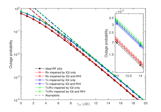
Fig 1: $P_{\text{out}}$ versus the normalized SNR over $\alpha-\mu$ fading channel
with $\alpha=2.3$ and $\mu=2.$

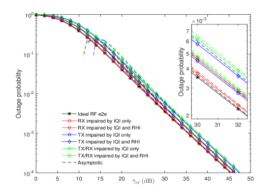
Fig 2: $P_{\text{out}}$ versus the normalized SNR over Málaga $\mathcal{M}$ turbulence channel
with $\alpha=2.296,\beta=2,\Omega=1,\rho=0.596,\Omega^{\prime}=1.3265$ and $\xi=3.85$.

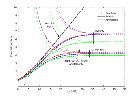
Fig 3: Channel capacity versus SNR over $\alpha-\mu$ fading channel
with $\alpha=3$ and $\mu=2.3$.

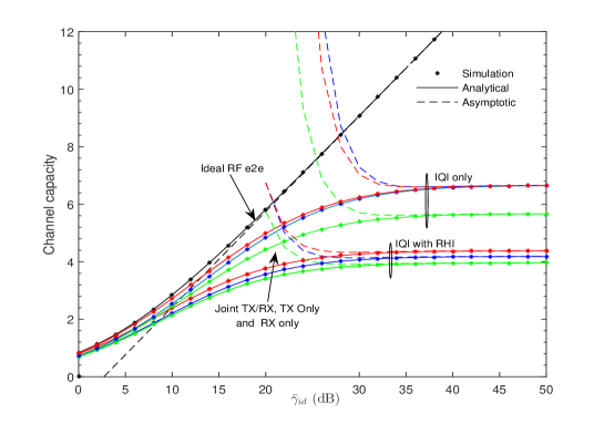
Fig 4: Channel capacity versus SNR over Málaga $\mathcal{M}$ turbulence channel
with $\alpha=2.296,\beta=2,\Omega=1,\rho=0.596,\Omega^{\prime}=1.3265$ and $\xi=3.85$.

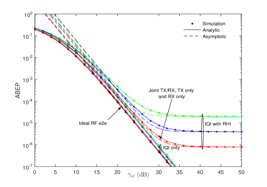
Fig 5: ASEP for GC-DQPSK over $\alpha-\mu$ fading channel with
$\alpha=2.3$ and $\mu=2$.

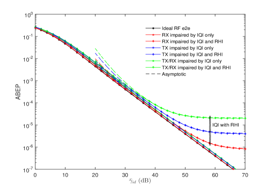
Fig 6: ASEP for GC-DQPSK over Málaga $\mathcal{M}$ turbulence channel with
$\alpha=2.296,\beta=2,\Omega=1,\rho=0.596,\Omega^{\prime}=1.3265$ and $\xi=3.85$.

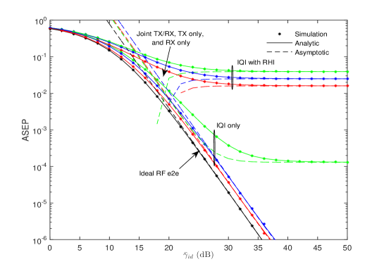
Fig 7: ASEP for $8-$PSK over $\alpha-\mu$ fading channel with
$\alpha=2.3$ and $\mu=2.$

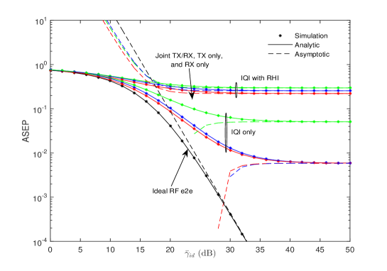
Fig 8: ASEP for $16-$PSK over $\alpha-\mu$ fading channel with
$\alpha=2.3$ and $\mu=2.$

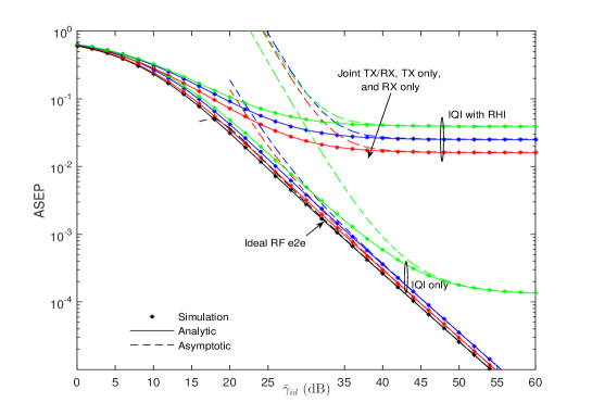
Fig 9: ASEP for $8-$PSK over Málaga $\mathcal{M}$ turbulence channel with
$\alpha=2.296,\beta=2,\Omega=1,\rho=0.596,\Omega^{\prime}=1.3265$ and $\xi=3.85$.

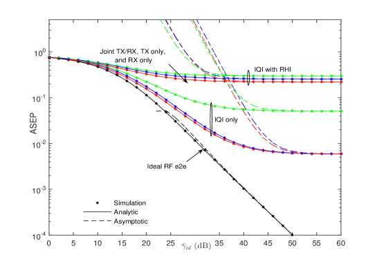
Fig 10: ASEP for $16-$PSK over Málaga $\mathcal{M}$ turbulence channel with
$\alpha=2.296,\beta=2,\Omega=1,\rho=0.596,\Omega^{\prime}=1.3265$ and $\xi=3.85$.

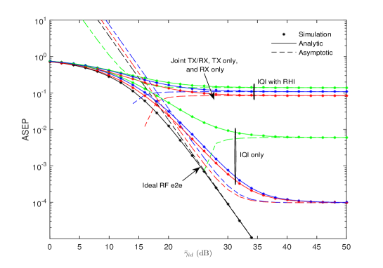
Fig 11: ASEP for $8-$DPSK over $\alpha-\mu$ fading channel with
$\alpha=2.3$ and $\mu=2.$

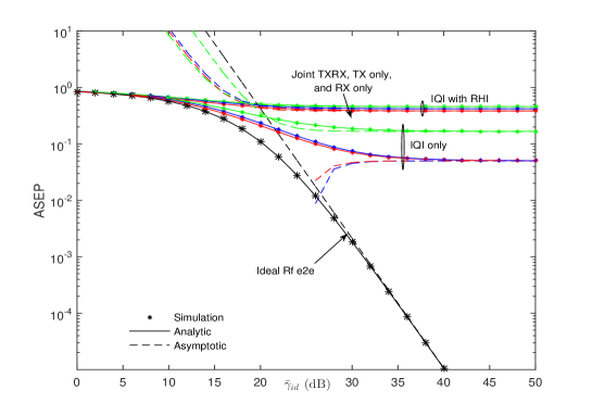
Fig 12: ASEP for $16-$DPSK over $\alpha-\mu$ fading channel with
$\alpha=2.3$ and $\mu=2.$

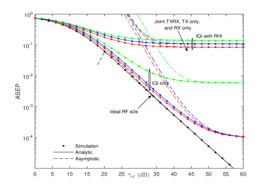
Fig 13: ASEP for $8-$DPSK over Málaga $\mathcal{M}$ turbulence channel with
$\alpha=2.296,\beta=2,\Omega=1,\rho=0.596,\Omega^{\prime}=1.3265$ and $\xi=3.85$.

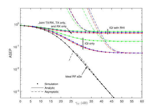
Fig 14: ASEP for $16-$DPSK over Málaga $\mathcal{M}$ turbulence channel with
$\alpha=2.296,\beta=2,\Omega=1,\rho=0.596,\Omega^{\prime}=1.3265$ and $\xi=3.85$.

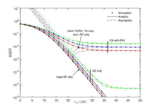
Fig 15: ASEP for $8-$QAM over $\alpha-\mu$ fading channel with
$\alpha=2.3$ and $\mu=2.$

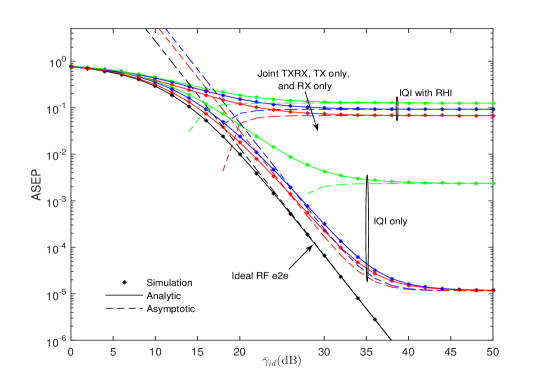
Fig 16: ASEP for $16-$QAM over $\alpha-\mu$ fading channel with
$\alpha=2.3$ and $\mu=2.$

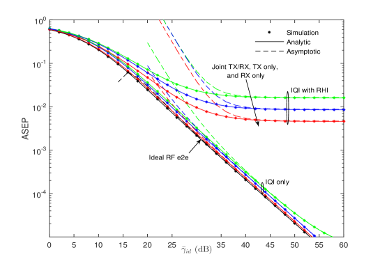
Fig 17: ASEP for $8-$QAM over Málaga $\mathcal{M}$ turbulence channel with
$\alpha=2.296,\beta=2,\Omega=1,\rho=0.596,\Omega^{\prime}=1.3265$ and $\xi=3.85$.

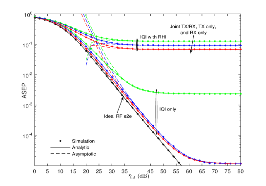
Fig 18: ASEP for $16-$QAM over Málaga $\mathcal{M}$ turbulence channel with
$\alpha=2.296,\beta=2,\Omega=1,\rho=0.596,\Omega^{\prime}=1.3265$ and $\xi=3.85$.

Appendix A: Proof of proposition 1

By setting $U^{\prime}=\frac{\partial F_{\gamma_{\varkappa}}\left(\gamma\right)}{\partial\gamma},$ $V=\log(1+\gamma)$, and using the integration by parts in $\left(\ref{ORAexpression}\right)$ with the help of $\left(\ref{CDFIQI}\right)$, one obtains

$$\mathcal{C}^{\left(\varkappa\right)} = \frac{1}{\log\left(2\right)}\sum_{\ell=1}^{L}\frac{\psi_{\ell}}{\phi_{\ell}}\int_{0}^{\frac{\omega_{\varkappa}}{\varrho_{\varkappa}}}\frac{1}{1+\gamma}{\small H}_{p+1{\small,q+1}}^{m+1{\small,n}}\left(\frac{\phi_{\ell}\tau_{\varkappa}\gamma}{\omega_{\varkappa}-\varrho_{\varkappa}\gamma}\left|\begin{array}[]{c}\Psi^{\left(\ell\right)}\\ \left(0,1\right),\Upsilon^{\left(\ell\right)}\end{array}\right.\right)d\gamma.$$ (88)

by plugging (6) into (88), we get

$$\mathcal{C}^{\left(\varkappa\right)} = \frac{1}{\log\left(2\right)}\frac{1}{2\pi j}\sum_{\ell=1}^{L}\frac{\psi_{\ell}}{\phi_{\ell}}\int_{\mathcal{L}_{v}^{\left(\ell\right)}}\frac{\prod\limits_{i=1}^{m}\Gamma\left(\mathcal{B}_{i}^{\left(\ell\right)}+B_{i}^{\left(\ell\right)}v\right)\prod\limits_{i=1}^{n}\Gamma\left(1-\mathcal{A}_{i}^{\left(\ell\right)}-A_{i}^{\left(\ell\right)}v\right)}{v\prod\limits_{i=n+1}^{p}\Gamma\left(\mathcal{A}_{i}^{\left(\ell\right)}+A_{i}^{\left(\ell\right)}v\right)\prod\limits_{i=m+1}^{q}\Gamma\left(1-\mathcal{B}_{i}^{\left(\ell\right)}-B_{i}^{\left(\ell\right)}v\right)}$$ (89)

$$\times\left(\frac{\phi_{\ell}\tau_{\varkappa}}{\varrho_{\varkappa}}\right)^{-v}\underbrace{\int_{0}^{\frac{\omega_{\varkappa}}{\varrho_{\varkappa}}}\gamma^{-v}\left(1+\gamma\right)^{-1}\left(\frac{\omega_{\varkappa}}{\varrho_{\varkappa}}-\gamma\right)^{v}d\gamma}_{\mathcal{I}_{\varkappa}}dv.$$

Further, the inner integral $\mathcal{I}_{\varkappa}$ can be evaluated using [35, Eq.(3.197.8)] as

$$\mathcal{I}_{\varkappa}\mathcal{=}\frac{\omega_{\varkappa}}{\varrho_{\varkappa}}\Gamma\left(1+v\right)\Gamma\left(1-v\right)\text{ }_{2}F_{1}\left(1,1-v;2;-\frac{\omega_{\varkappa}}{\varrho_{\varkappa}}\right),$$ (90)

where ${}_{2}F_{1}\left(.,.;.;.\right)$ denotes the Gauss hypergeometric function (GHF) [35, Eq. (9.100)].
Now plugging $\left(\ref{innerintegral}\right)$ into $\left(\ref{ORAdetail}\right)$ and using the integral Mellin-Barnes representation of the GHF [35, Eq. (9.113)], yields

$$\mathcal{C}^{\left(\varkappa\right)} = \frac{1}{\log(2)}\left(\frac{1}{2\pi j}\right)^{2}\sum_{\ell=1}^{L}\frac{\psi_{\ell}}{\phi_{\ell}}\int_{\mathcal{L}_{v}^{\left(\ell\right)}}\int_{\mathcal{L}_{w}^{\left(\ell\right)}}\frac{\Gamma\left({-v-w}\right)\Gamma\left(v\right)\prod\limits_{i=1}^{m}\Gamma\left(\mathcal{B}_{i}^{\left(\ell\right)}+B_{i}^{\left(\ell\right)}v\right)\prod\limits_{i=1}^{n}\Gamma\left(1-\mathcal{A}_{i}^{\left(\ell\right)}-A_{i}^{\left(\ell\right)}v\right)}{\prod\limits_{i=n+1}^{p}\Gamma\left(\mathcal{A}_{i}^{\left(\ell\right)}+A_{i}^{\left(\ell\right)}v\right)\prod\limits_{i=m+1}^{q}\Gamma\left(1-\mathcal{B}_{i}^{\left(\ell\right)}-A_{i}^{\left(\ell\right)}v\right)}$$ (91)

$$\times\frac{\Gamma\left(1+w\right)\Gamma\left({-w}\right)}{\Gamma\left(1-w\right)}\left(\frac{\phi_{\ell}\tau_{\varkappa}}{\varrho_{\varkappa}}\right)^{-v}\left(\frac{\omega_{\varkappa}}{\varrho_{\varkappa}}\right)^{-w}dvdw,$$

which concludes the proof of Proposition 1.

Appendix B: Proof of corollary 50

By replacing $\omega_{\varkappa}=\tau_{\varkappa}=1$ in $\left(\ref{ORRA}\right)$, the CC under ORA policy can be simplified to

$$\mathcal{C}^{\left(\varkappa\right)} = \frac{1}{\log(2)}\left(\frac{1}{2\pi j}\right)^{2}\sum_{\ell=1}^{L}\frac{\psi_{\ell}}{\phi_{\ell}}\int_{\mathcal{L}_{v}^{\left(\ell\right)}}\int_{\mathcal{L}_{w}^{\left(\ell\right)}}\frac{\Gamma\left(-v-w\right)\Gamma\left(v\right)\prod\limits_{i=1}^{m}\Gamma\left(\mathcal{B}_{i}^{\left(\ell\right)}+B_{i}^{\left(\ell\right)}v\right)}{\prod\limits_{i=n+1}^{p}\Gamma\left(\mathcal{A}_{i}^{\left(\ell\right)}+A_{i}^{\left(\ell\right)}v\right)}$$

$$\times\frac{\prod\limits_{i=1}^{n}\Gamma\left(1-\mathcal{A}_{i}^{\left(\ell\right)}-A_{i}^{\left(\ell\right)}v\right)}{\prod\limits_{i=m+1}^{q}\Gamma\left(1-\mathcal{B}_{i}^{\left(\ell\right)}-B_{i}^{\left(\ell\right)}v\right)}\frac{\Gamma\left(-w\right)\Gamma\left(1+w\right)}{\Gamma\left(1-w\right)}\phi_{\ell}^{-v}\left(\frac{1}{\varrho_{\varkappa}}\right)^{-w-v}dvdw.$$

Using the change of variable $s=$ $-w-v,$ we get

$$\mathcal{C}^{\left(\varkappa\right)} = \frac{1}{\log(2)}\frac{1}{2\pi j}\sum_{\ell=1}^{L}\frac{\psi_{\ell}}{\phi_{\ell}}\int_{\mathcal{L}_{v}^{\left(\ell\right)}}\frac{\Gamma\left(v\right)\prod\limits_{i=1}^{m}\Gamma\left(\mathcal{B}_{i}^{\left(\ell\right)}+B_{i}^{\left(\ell\right)}v\right)\prod\limits_{i=1}^{n}\Gamma\left(1-\mathcal{A}_{i}^{\left(\ell\right)}-A_{i}^{\left(\ell\right)}v\right)}{\prod\limits_{i=n+1}^{p}\Gamma\left(\mathcal{A}_{i}^{\left(\ell\right)}+A_{i}^{\left(\ell\right)}v\right)\prod\limits_{i=m+1}^{q}\Gamma\left(1-\mathcal{B}_{i}^{\left(\ell\right)}-B_{i}^{\left(\ell\right)}v\right)}\phi_{\ell}^{-v}$$ (92)

$$\times\underbrace{\frac{1}{2\pi j}\int_{\mathcal{L}_{s}^{\left(\ell\right)}}\frac{\Gamma\left(s+v\right)\Gamma\left(1-s-v\right)}{\Gamma\left(1+s+v\right)}\Gamma\left(s\right)\varrho_{\varkappa}^{-s}ds}_{\mathcal{K}_{\varkappa}}dv$$

For significantly smaller values of $\varrho_{\varkappa}$ (i.e., $\varrho_{\varkappa}<<1$), the condition [22, Eq. (1.2.15)] is satisfied. It follows that the inner integral $\mathcal{K}_{\varkappa}$ can be expressed as an infinite summation of the residues evaluated at the left poles. Subsequently, relying on [22, Theorem 1.3], $\mathcal{K}_{\varkappa}$ can be expressed as

$$\mathcal{K}_{\varkappa}\mathcal{=}\sum_{l=0}^{\infty}\frac{\left(-1\right)^{l}\Gamma\left(-l+v\right)\Gamma\left(1+l-v\right)}{l!\Gamma\left(1-l+v\right)}\varrho_{\varkappa}^{l}.$$ (93)

Particularly, for $\varrho_{\varkappa}=0$ (i.e., case of ideal RF e$2$e), $\left(\ref{K-residu}\right)$ is reduced to

$$\mathcal{K}_{\varkappa}\mathcal{=}\frac{\Gamma\left(v\right)\Gamma\left(1-v\right)}{\Gamma\left(1+v\right)}.$$ (94)

Thus, the CC under ORA policy and ideal RF e$2$e can be expressed as

$$\mathcal{C}^{\left(\varkappa\right)} = \frac{1}{\log(2)}\sum_{\ell=1}^{L}\frac{\psi_{\ell}}{\phi_{\ell}}\left(\frac{1}{2\pi j}\right)\int_{\mathcal{L}_{v}^{\left(\ell\right)}}\frac{\Gamma\left(v\right)\Gamma\left(v\right)\Gamma\left(1-v\right)}{\Gamma\left(1+v\right)}$$ (95)

$$\times\frac{\prod\limits_{i=1}^{m}\Gamma\left(\mathcal{B}_{i}^{\left(\ell\right)}+B_{i}^{\left(\ell\right)}v\right)\prod\limits_{i=1}^{n}\Gamma\left(1-\mathcal{A}_{i}^{\left(\ell\right)}-A_{i}^{\left(\ell\right)}v\right)}{\prod\limits_{i=n+1}^{p}\Gamma\left(\mathcal{A}_{i}^{\left(\ell\right)}+A_{i}^{\left(\ell\right)}v\right)\prod\limits_{i=m+1}^{q}\Gamma\left(1-\mathcal{B}_{i}^{\left(\ell\right)}-B_{i}^{\left(\ell\right)}v\right)}\phi_{\ell}^{-v}dv.$$

This concludes the proof.

Appendix C: Proof of proposition 3

By substituting $\left(\ref{SEPbin}\right)$ into the following equation

$$P_{s}^{\left(\varkappa\right)}=\int_{0}^{\frac{\omega_{\varkappa}}{\varrho_{\varkappa}}}\mathcal{H}\left(\gamma\right)\frac{\partial F_{\gamma_{\varkappa}}\left(\gamma\right)}{\partial\gamma}d\gamma,$$ (96)

one gets a tight approximate formula

$$P_{s}^{\left(\varkappa\right)}\simeq\sum_{n=0}^{N}\theta_{n}\mathcal{I}_{n}^{\left(\varkappa\right)},$$ (97)

with

$$\mathcal{I}_{n}^{\left(\varkappa\right)}=\int_{0}^{\frac{\omega_{\varkappa}}{\varrho_{\varkappa}}}\exp\left(-\delta_{n}\gamma\right)\frac{\partial F_{\gamma_{\varkappa}}\left(\gamma\right)}{\partial\gamma}d\gamma.$$ (98)

By setting $U^{\prime}=\frac{\partial F_{\gamma_{\varkappa}}\left(\gamma\right)}{\partial\gamma}$, $V=\exp\left(-\delta_{n}\gamma\right)$, and using $\left(\ref{CDFIQI}\right)$, one can obtain

$$\mathcal{I}_{n}^{\left(\varkappa\right)} = 1-\delta_{n}\sum_{\ell=1}^{L}\frac{\psi_{\ell}}{\phi_{\ell}}\int_{0}^{\frac{\omega_{\varkappa}}{\varrho_{\varkappa}}}\exp\left(-\delta_{n}\gamma\right)$$ (101)

$$\times{\small H}_{p+1{\small,q+1}}^{m+1{\small,n}}\left(\frac{\phi_{\ell}\tau_{\varkappa}\gamma}{\omega_{\varkappa}-\varrho_{\varkappa}\gamma}\left|\begin{array}[]{c}\left(\mathcal{A}_{i}^{\left(\ell\right)},A_{i}^{\left(\ell\right)}\right)_{i=1:p},\left(1,1\right)\\ \left(0,1\right),\left(\mathcal{B}_{i}^{\left(\ell\right)},B_{i}^{\left(\ell\right)}\right)_{i=1:q}\end{array}\right.\right)d\gamma.$$

Subsequently, $\left(\ref{EqIntegral-n}\right)$ can be rewritten with the help of $\left(\ref{Hffox}\right)$ as

$$\mathcal{I}_{n}^{\left(\varkappa\right)} = 1-\frac{\delta_{n}}{2\pi j}\sum_{\ell=1}^{L}\frac{\psi_{\ell}}{\phi_{\ell}}\int_{\mathcal{L}_{v}^{\left(\ell\right)}}\frac{\prod\limits_{i=1}^{m}\Gamma\left(\mathcal{B}_{i}^{\left(\ell\right)}+B_{i}^{\left(\ell\right)}v\right)\prod\limits_{i=1}^{n}\Gamma\left(1-\mathcal{A}_{i}^{\left(\ell\right)}-A_{i}^{\left(\ell\right)}v\right)}{v\prod\limits_{i=n+1}^{p}\Gamma\left(\mathcal{A}_{i}^{\left(\ell\right)}+A_{i}^{\left(\ell\right)}v\right)\prod\limits_{i=m+1}^{q}\Gamma\left(1-\mathcal{B}_{i}^{\left(\ell\right)}-B_{i}^{\left(\ell\right)}v\right)}$$ (103)

$$\times\left(\frac{\phi_{\ell}\tau_{\varkappa}}{\varrho_{\varkappa}}\right)^{-v}\underbrace{\int_{0}^{\frac{\omega_{\varkappa}}{\varrho_{\varkappa}}}\gamma^{-v}\left(\frac{\omega_{\varkappa}}{\varrho_{\varkappa}}-\gamma\right)^{v}\exp\left(-\delta_{n}\gamma\right)d\gamma}_{\mathcal{J}_{\varkappa}}dv.$$

whereas the inner integral $\mathcal{J}_{\varkappa}$ can be evaluated using [35, Eq. (3.383.1)] as

$$\mathcal{J}_{\varkappa}\mathcal{=}\Gamma\left(1+v\right)\frac{\omega_{\varkappa}}{\varrho_{\varkappa}}\text{ }_{1}F_{1}\left(1-v;2;-\frac{\delta_{n}\omega_{\varkappa}}{\varrho_{\varkappa}}\right),$$ (104)

where ${}_{1}F_{1}\left(.;.;.\right)$ denotes the confluent hypergeometric function [35, Eq. (9.21)]. Lastly, plugging $\left(\ref{J_integral}\right)$ into $\left(\ref{integ2}\right)$ and using [22, Eqs. (2.9.14)] along with (6), yields

$$\mathcal{I}_{n}^{\left(\varkappa\right)} = 1-\left(\frac{1}{2\pi j}\right)^{2}\sum_{\ell=1}^{L}\frac{\psi_{\ell}}{\phi_{\ell}}\int_{\mathcal{L}_{v}^{\left(\ell\right)}}\int_{\mathcal{L}_{s}^{\left(\ell\right)}}\Gamma\left(-v-s\right)\frac{\Gamma\left(v\right)\prod\limits_{i=1}^{m}\Gamma\left(\mathcal{B}_{i}^{\left(\ell\right)}+B_{i}^{\left(\ell\right)}v\right)}{\prod\limits_{i=n+1}^{p}\Gamma\left(\mathcal{A}_{i}^{\left(\ell\right)}+A_{i}^{\left(\ell\right)}v\right)}$$ (105)

$$\times\frac{\prod\limits_{i=1}^{n}\Gamma\left(1-\mathcal{A}_{i}^{\left(\ell\right)}-A_{i}^{\left(\ell\right)}v\right)}{\prod\limits_{i=m+1}^{q}\Gamma\left(1-\mathcal{B}_{i}^{\left(\ell\right)}-B_{i}^{\left(\ell\right)}v\right)}\frac{\Gamma\left(1+s\right)}{\Gamma\left(1-s\right)}\left(\frac{\phi_{\ell}\tau_{\varkappa}}{\varrho_{\varkappa}}\right)^{-v}\left(\frac{\delta_{n}\omega_{\varkappa}}{\varrho_{\varkappa}}\right)^{-s}dvds,$$

which concludes the proof.

Appendix D: Proof of corollary 2

By setting $\omega_{\varkappa}=\tau_{\varkappa}=1,\left(\ref{Integral_n}\right)$ can be rewritten using the change of variable $w=-s-v$ as

$$\mathcal{I}_{n}^{\left(\varkappa\right)} = 1-\frac{1}{2\pi j}\sum_{\ell=1}^{L}\frac{\psi_{\ell}}{\phi_{\ell}}\int_{\mathcal{L}_{v}^{\left(\ell\right)}}\frac{\Gamma\left(v\right)\prod\limits_{i=1}^{m}\Gamma\left(\mathcal{B}_{i}^{\left(\ell\right)}+B_{i}^{\left(\ell\right)}v\right)\prod\limits_{i=1}^{n}\Gamma\left(1-\mathcal{A}_{i}^{\left(\ell\right)}-A_{i}^{\left(\ell\right)}v\right)}{\prod\limits_{i=n+1}^{p}\Gamma\left(\mathcal{A}_{i}^{\left(\ell\right)}+A_{i}^{\left(\ell\right)}v\right)\prod\limits_{i=m+1}^{q}\Gamma\left(1-\mathcal{B}_{i}^{\left(\ell\right)}-B_{i}^{\left(\ell\right)}v\right)}$$ (106)

$$\times\left(\frac{\phi_{\ell}}{\delta_{n}}\right)^{-v}\underbrace{\frac{1}{2\pi j}\int_{\mathcal{L}_{w}^{\left(\ell\right)}}\Gamma\left(w\right)\frac{\Gamma\left(1-w-v\right)}{\Gamma\left(1+w+v\right)}\left(\frac{\varrho_{\varkappa}}{\delta_{n}}\right)^{w}dw}_{\mathcal{M}_{\varkappa}}dv.$$

Again, for significantly smaller values of $\varrho_{\varkappa}$ (i.e., $\varrho_{\varkappa}<<1$) and similarly to $\mathcal{K}_{\varkappa}$, the inner integral $\mathcal{M}_{\varkappa}$ can be expressed as

$$\mathcal{M}_{\varkappa}\mathcal{=}\sum_{l=0}^{\infty}\frac{\left(-1\right)^{l}\Gamma\left(1+l-v\right)}{l!\Gamma\left(1-l+v\right)}\left(\frac{\varrho_{\varkappa}}{\delta_{n}}\right)^{l}.$$ (107)

Specifically, for $\varrho_{\varkappa}=0$, $\left(\ref{M-residu}\right)$ is reduced to

$$\mathcal{M}_{\varkappa}\mathcal{=}\frac{\Gamma\left(1-v\right)}{\Gamma\left(1+v\right)}.$$ (108)

As a result, $\left(\ref{Integrall-n}\right)$ can be reexpressed by incorporating $\left(\ref{M-res2}\right)$ as

$$\mathcal{I}_{n}^{\left(\varkappa\right)} = 1-\frac{1}{2\pi j}\sum_{\ell=1}^{L}\frac{\psi_{\ell}}{\phi_{\ell}}\int_{\mathcal{L}_{v}^{\left(\ell\right)}}\frac{\Gamma\left(v\right)\prod\limits_{i=1}^{m}\Gamma\left(\mathcal{B}_{i}^{\left(\ell\right)}+B_{i}^{\left(\ell\right)}v\right)}{\Gamma\left(1+v\right)\prod\limits_{i=n+1}^{p}\Gamma\left(\mathcal{A}_{i}^{\left(\ell\right)}+A_{i}^{\left(\ell\right)}v\right)}$$ (109)

$$\times\frac{\Gamma\left(1-v\right)\prod\limits_{i=1}^{n}\Gamma\left(1-\mathcal{A}_{i}^{\left(\ell\right)}-A_{i}^{\left(\ell\right)}v\right)}{\prod\limits_{i=m+1}^{q}\Gamma\left(1-\mathcal{B}_{i}^{\left(\ell\right)}-B_{i}^{\left(\ell\right)}v\right)}\left(\frac{\phi_{\ell}}{\delta_{n}}\right)^{-v}dv.$$

Thus, the proof is concluded.

Appendix E: Proof of proposition 4

By plugging $\left(\ref{ApproFHF}\right)$ in $\left(\ref{EqIntegral-n}\right)$ and using [22, Eq. (2.9.4)], yields the following approximate expression in the high SNR regime

$$\mathcal{I}_{n}^{\left(\varkappa\right)} \sim 1-\sum_{\ell=1}^{L}\frac{\psi_{\ell}}{\phi_{\ell}}E_{\ell}\left[1-\exp\left(-\frac{\delta_{n}\omega_{\varkappa}}{\varrho_{\varkappa}}\right)\right]+\delta_{n}\sum_{\ell=1}^{L}\frac{\psi_{\ell}}{\phi_{\ell}}\sum_{i=1}^{m}\mathcal{F}_{\ell,i}\left(\frac{\phi_{\ell}\tau_{\varkappa}}{\omega_{\varkappa}}\right)^{\frac{\mathcal{B}_{i}^{\left(\ell\right)}}{B_{i}^{\left(\ell\right)}}}$$ (110)

$$\times\frac{1}{2\pi j}\int_{\mathcal{L}_{s}^{\left(\ell\right)}}\Gamma\left(s\right)\left(\delta_{n}\right)^{-s}\int_{0}^{\frac{\omega_{\varkappa}}{\varrho_{\varkappa}}}\gamma^{\frac{\mathcal{B}_{i}^{\left(\ell\right)}}{B_{i}^{\left(\ell\right)}}-s}\left(1-\frac{\varrho_{\varkappa}}{\omega_{\varkappa}}\gamma\right)^{\frac{\mathcal{B}_{i}^{\left(\ell\right)}}{B_{i}^{\left(\ell\right)}}}d\gamma ds.$$

Now, using $\left(\ref{Hffox}\right)$, [22, Eq. (2.9.15)], and [35, Eq. (1.3.194)], one obtains

$$\mathcal{I}_{n}^{\left(\varkappa\right)} \sim \exp\left(-\frac{\delta_{n}\omega_{\varkappa}}{\varrho_{\varkappa}}\right)+\delta_{n}\sum_{\ell=1}^{L}\frac{\psi_{\ell}\omega_{\varkappa}}{\phi_{\ell}\varrho_{\varkappa}}\sum_{i=1}^{m}\frac{\mathcal{F}_{\ell,i}\left(\frac{\phi_{\ell}\tau_{\varkappa}}{\omega_{\varkappa}}\right)^{\frac{\mathcal{B}_{i}^{\left(\ell\right)}}{B_{i}^{\left(\ell\right)}}}}{\Gamma\left(\frac{\mathcal{B}_{i}}{B_{i}}\right)}\left(\frac{1}{2\pi j}\right)^{2}\int_{\mathcal{L}_{s}^{\left(\ell\right)}}\int_{\mathcal{L}_{v}^{\left(\ell\right)}}\Gamma\left(s\right)\Gamma\left(v\right)$$ (111)

$$\times\frac{\Gamma\left(1+\frac{\mathcal{B}_{i}^{\left(\ell\right)}}{B_{i}^{\left(\ell\right)}}-s-v\right)}{\Gamma\left(2+\frac{\mathcal{B}_{i}^{\left(\ell\right)}}{B_{i}^{\left(\ell\right)}}-s-v\right)}\Gamma\left(\frac{\mathcal{B}_{i}^{\left(\ell\right)}}{B_{i}^{\left(\ell\right)}}-v\right)\left(\frac{\delta_{n}\omega_{\varkappa}}{\varrho_{\varkappa}}\right)^{-s}\left(-1\right)^{-v}dsdv.$$

Finally, substituting (111) into (97), yields (81), which concludes the proof.

References

• [1] S. Mirabbasi and K. Martin, “Classical and modern receiver architectures,” IEEE Commun. Mag., vol. 38, no. 11, pp. 132-139, Nov. 2000.
• [2] Crols, Jan, and Michiel Steyaert. CMOS wireless transceiver design. vol. 411. Springer Science and Business Media, 2013.
• [3] T. Schenk, RF imperfections in high-rate wireless systems: impact and digital compensation. Springer Science and Business Media, 2008.
• [4] T. H. Nguyen et al., “Blind transmitter I/Q imbalance compensation in $M$-QAM optical coherent systems,” J. Opt. Commun. Netw., vol. 9, no. 9, pp. 42-50, Sep. 2017.
• [5] B. Selim et al., “Performance analysis of single-carrier coherent and noncoherent modulation under I/Q imbalance,” in Proc. IEEE 87th Veh. Technolo. Conf. (VTC Spring), Jun. 2018, pp. 1-5.
• [6] J. Li, M. Matthaiou, and T. Svensson, “I/Q imbalance in AF dual-hop relaying: Performance analysis in Nakagami-$m$ fading,” IEEE Trans. Commun., vol. 62, no. 3, pp. 836-847, Mar. 2014.
• [7] A. E. Canbilen et al., “Impact of I/Q imbalance on amplify-and-forward relaying: Optimal detector design and error performance,” IEEE Trans. Commun., vol. 67, no. 5, pp. 3154-3166, May 2019.
• [8] P. Song, N. Zhang and F. Gong, “Blind estimation algorithms for I/Q imbalance in direct down-conversion receivers,” in Proc. 2018 IEEE 88th Veh. Technology Conf. (VTC-Fall), Chicago, IL, USA, Aug. 2018, pp. 1-5.
• [9] Q. Zhang et al., “Algorithms for blind separation and estimation of transmitter and receiver IQ imbalances,” Journal of Lightwave Technology, vol. 37, no. 10, pp. 2201-2208, May 2019.
• [10] ] M. Valkama, M. Renfors, and V. Koivune, “Advanced methods for I/Q imbalance compensation in communication receivers,” IEEE Trans. Signal Process., vol. 49, no. 10, pp. 2335-2344, Oct. 2001.
• [11] J. Luo, A. Kortke, W. Keusgen, and M. Valkama, “A novel adaptive calibration scheme for frequency-selective I/Q imbalance in broadband direct-conversion transmitters,” in IEEE Trans. Circuits and Systems II, Express Briefs, vol. 60, no. 2, pp. 61-65, Feb. 2013.
• [12] J. Kim et al., “A low-complexity I/Q imbalance calibration method for quadrature modulator,” IEEE Trans. On Very Large Scale Integration Systems, vol. 27, no. 4, pp. 974-977, Apr. 2019.
• [13] P. K. Sharma and P. K. Upadhyay, “Cognitive relaying with transceiver hardware impairments under interference constraints,” IEEE Commun. Lett., vol. 20, no. 4, pp. 820-823, Apr. 2016.
• [14] A. K. Mishra, D. Mallick, and P. Singh, “Combined effect of RF impairment and CEE on the performance of dual-hop fixed-gain AF relaying,” IEEE Trans. Lett., vol. 20, no. 9, pp. 1725-1728, Sep. 2016.
• [15] K. Guo, B. Zhang, Y. Huang, and D. Guo, “Outage analysis of multi-relay networks with hardware impairments using SECps scheduling scheme in shadowed-Rician channel,” IEEE Access, vol. 5, pp. 5113-5120, Mar. 2017.
• [16] F. Ding, H. Wang, S. Zhang, and M. Dai, “Impact of residual hardware impairments on non-orthogonal multiple access based amplify-and-forward relaying networks,” IEEE Access, vol. 6, pp. 15117-15131, Mar. 2018.
• [17] F. El Bouanani, Y. Mouchtak, and G. K. Karagiannidis, “New tight bounds for the Gaussian $Q$-function and applications,” IEEE Access, vol. 8, pp. 145037-145055, Sep. 2020.
• [18] C. D. Bodenschatz, Finding an H-function distribution for the sum of independent H-function variates. Ph.D. thesis, The University of Texas, Austin, Tx, May. 1992.
• [19] F. El Bouanani and D. B. da Costa, “Accurate closed-form approximations for the sum of correlated Weibull random variables,” IEEE Wireless Commun. Lett., vol. 7, no. 4, pp. 498-501, Aug. 2018.
• [20] E. Illi, F. El Bouanani, and F. Ayoub, “On the distribution of the sum of Málaga-$M$ random variables and applications,” IEEE Trans. Veh. Technol., vol. 69, no. 11, pp. 13996-14000, Oct. 2020.
• [21] F. El Bouanani, S. Muhaidat, P. C. Sofotasios, O. Dobre, and O. S. Bardaneh, “Performance analysis of intelligent reflecting surface aided wireless networks with wireless power transfer,” IEEE Commun. Lett., vol. 25, no. 3, pp. 793-797, Mar. 2021
• [22] A. Kilbas and M. Saigo, H-Transforms: Theory and Applications. Boca Raton, Florida, USA: CRC Press LLC, 2004.
• [23] L. Kong, G. Kaddoum, and H. Chergui, “On physical layer security over Fox’s $H$-Function wiretap fading channels,” IEEE Trans. Veh. Technol., vol. 68, no. 7, pp. 6608-6621, May 2019.
• [24] M. K. Simon and M.-S. Alouini, Digital communications over fading channels, 2nd edition, John Wiley & Sons, 2005.
• [25] A. Annamalai, and C. Tellambura, “Error rates for Nakagami-$m$ fading multichannel reception of binary and $M$-ary signals,” IEEE Trans. Commun., vol. 49, no. 1, pp. 58-68, Jan. 2001.
• [26] Y. Mouchtak and F. El Bouanani, “New Accurate Approximation for Average Error Probability,” IEEE Access, vol. 9, pp. 4388-4397, Dec. 2020.
• [27] M. Lupupa and J. Qi, “I/Q imbalance in generalized frequency division multiplexing under Weibull fading,” in Proc. IEEE PIMRC’15, Aug 2015, pp. 471-476.
• [28] B. Selim, P. C. Sofotasios, et al., “Performance of differential modulation under RF impairments,” in Proc. IEEE International Conf. on Commun. (ICC), May 2017, pp. 1-6.
• [29] A. A. Boulogeorgos et al., “Effects of RF impairments in communications over cascaded fading channels,” IEEE Trans. Veh. Technol., vol. 65, no. 11, pp. 8878-8894, Nov. 2016.
• [30] C. Zhu, J. Cheng, and N. Al-Dhahir, “Error rate analysis of subcarrier QPSK with receiver I/Q imbalances over Gamma-Gamma fading channels,” in Proc. Int. Conf. Comput., Netw. Commun. (ICNC), Jan. 2017, pp. 88-94.
• [31] J. Abouei, K. N. Plataniotis, and S. Pasupathy, “Green modulations in energy-constrained wireless sensor networks,” IET Commun., vol. 5, no. 2, pp. 240-251, Jan. 2011.
• [32] HK Gill, GK Walia and NS Grewal, “Performance analysis of mode division multiplexing IS-OWC system using Manchester, DPSK and DQPSK modulation techniques,” Optik., vol. 177, pp. 93-101, Jan. 2019.
• [33] A. Mathai, R. K. Saxena, and H. Haubold, The H Function: Theory and Applications. New York: Springer, 2010.
• [34] F. Yilmaz and M.-S. Alouini, “A novel unified expression for the capacity and bit error probability of wireless communication systems over generalized fading channels,” IEEE Trans. Commun., vol. 60, no.7, pp. 1862-1876, Jul. 2012.
• [35] A. Jeffrey and D. Zwillinger, Table of integrals, series, and products. Elsevier, 2007.
• [36] B. Razavi, RF microelectronics. vol. 2. New York: Prentice-Hall, 2012.
• [37] C. Studer, M. Wenk, and A. Burg, “MIMO transmission with residual transmit-RF impairments,” International ITG Workshop on Smart Antennas, Bremen, Germany, 2010, pp. 189-196.
• [38] M. Abramowitz and I. A. Stegun (Eds), Handbook of Mathematical Functions with Formulas, Graphs, and Mathematical Tables, National Bureau of Standards, Applied Mathematics Series 55, Washington, 1970.
• [39] E. Illi, F. El Bouanani, and F. Ayoub, “A performance study of a hybrid 5G RF/FSO transmission system,” in Proc. Con on Wireless Networks and Mobile Communications (WINCOM), Nov. 2017, pp. 1-7.