The VMC Survey - XLII. Near-infrared period-luminosity relations for RR Lyrae stars and the structure of the Large Magellanic Cloud.

Abstract

We present results from an analysis of $\sim$ 29,000 RR Lyrae stars located in the Large Magellanic Cloud (LMC). For these objects, near-infrared time-series photometry from the VISTA survey of the Magellanic Clouds system (VMC) and optical data from the OGLE (Optical Gravitational Lensing Experiment) IV survey and the Gaia Data Release 2 catalogue of confirmed RR Lyrae stars were exploited. Using VMC and OGLE IV magnitudes we derived period–luminosity (PL), period–luminosity–metallicity (PLZ), period–Wesenheit (PW) and period–Wesenheit–metallicity (PWZ) relations in all available bands. More that  7,000 RR Lyrae were discarded from the analysis because they appear to be overluminous with respect to the PL relations. The $PL_{K_{\mathrm{s}}}$ relation was used to derive individual distance to $\sim 22,000$ RR Lyrae stars, and study the three-dimensional structure of the LMC. The distribution of the LMC RR Lyrae stars is ellipsoidal with the three axis $S_{1}$=6.5 kpc, $S_{2}$=4.6 kpc and $S_{3}$=3.7 kpc, inclination i=$22\pm 4^{\circ}$ relative to the plane of the sky and position angle of the line of nodes $\theta=167\pm 7^{\circ}$ (measured from north to east). The north-eastern part of the ellipsoid is closer to us and no particular associated substructures are detected as well as any metallicity gradient.

1 Introduction

Among the oldest objects in the Universe ($t>10$ Gyr) RR Lyrae stars (RRLs) are pulsating variables with low masses (M$\leq$0.85 M_⊙) and helium-burning cores, which place them on the horizontal branch (HB) evolutionary sequence. RRLs are one of the most numerous type of pulsating stars, commonly found in globular clusters (GCs) and in galaxies hosting an old stellar component. The visual absolute magnitude of RRLs does not vary significantly with period, because these variables are found on the HB, but has been found and predicted to depend on metallicity according to a luminosity–metallicity relation (M_V–[Fe/H]) which is fundamental for the use of RRLs as primary distance indicators (van Albada & Baker 1971; Sandage 1981a, b). On the other hand, the dependence of the $V$–$K$ colour on effective temperature leads to the occurrence of a near-infrared (NIR) Period–Luminosity–Metallicity ($PLZ$) relation for RRLs, first empirically observed by Longmore et al. (1986). As comprehensively discussed by Nemec et al. (1994), the effect of reddening is significantly reduced in the NIR compared with optical wavelengths (A_Ks/A${}_{V}\sim 1/9$, Cardelli et al., 1989) and the amplitude of pulsation is smaller than in the optical (Amp_Ks/Amp${}_{V}\sim 1/4$, e. g. Braga et al., 2018), allowing the derivation of precise mean magnitudes even based on a limited number of observations. This makes the RRL $PLZ$ NIR relations an even more powerful tool to measure distances than its optical counterparts. Moreover, tighter relations are derived by introducing a colour term to the $PL$ relation. In particular the Wesenheit function (van den Bergh, 1975; Madore, 1982) includes a color term whose coefficient is equal to the ratio of the total-to-selective extinction in a filter pair [$W(X,Y)=X-R_{X}\times(X-Y)$]. As such the period-Wesenheit (PW) relation is reddening-free by definition.

The Large Magellanic Cloud (LMC) is a dwarf irregular galaxy hosting several different stellar populations from old, to intermediate, to young, as well as a number of star forming regions. It is one of the closest companions of the Milky Way and the first rung of the astronomical distance ladder. Along with the Small Magellanic Cloud (SMC), the LMC is part of the Magellanic System which also comprises the Bridge connecting the two Clouds and the Magellanic Stream. The RRLs trace the oldest stellar component and probe the structure of the LMC and SMC haloes, as opposed to Classical Cepheids (CCs), which trace regions of recent star formation like the LMC bar and spiral arms (Moretti et al., 2014).

The Magellanic RRLs have been observed in optical passbands and catalogued systematically by a number of different microlensing surveys: the Massive Compact Halo Objects survey (MACHO; Alcock et al. 1997), the Optical Gravitational Lensing Experiment (OGLE; Udalski et al. 1997; Soszyński et al. 2016, 2019), the Experiénce pour la Recherche d’Objets Sombres 2 survey (EROS-2; Tisserand et al. 2007) and, most recently, by the $Gaia$ mission (Gaia Collaboration, et al. 2016a, b, 2018a and references therein). $Gaia$ is repeatedly monitoring the whole sky down to a limiting magnitude $G\sim$ 20.7–21 mag. By fully mapping the Magellanic System $Gaia$ is increasing the census of RRLs, revealing the whole extension of the LMC and SMC haloes as well of the Bridge region (see, e.g. figs. 42 and 43 of Clementini et al. 2019). About 2000 new RRLs published in the Gaia Data Release 2 (DR2; Clementini et al. 2019) were discovered in the Magellanic System; about 850 are outside and the remaining 1150 are inside the OGLE footprint as described by Soszyński et al. (2019). Nevertheless, the RRL catalogues published by OGLE (e.g. Soszyński et al., 2009, 2012, 2016, 2019) still represent fundamental references for the Magellanic System RRLs, since they provide light curves in the standard Johnson–Cousins $V_{J},I_{C}$ passbands for about 48,000 of these variables, along with their pulsation period (P), mean magnitude and amplitude in the $I$ band, and the main Fourier parameters of their light curves.

At NIR wavelengths, an unprecedented step forward in our knowledge of the properties of the RRLs in the Magellanic System is being provided by the VISTA $Y,J,K_{\mathrm{s}}$ survey of the Magellanic Clouds system (VMC, Cioni et al. 2011). The survey aims at studying the star formation history (SFH) and the three-dimensional (3-D) structure of the LMC, the SMC, the Bridge and of a small section of the Magellanic Stream. The approach used to derive the SFH is based on a combination of model single-burst populations that best describes the observed colour–magnitude diagrams (CMDs; see e.g., Rubele et al. 2012, 2015, 2018). The 3-D geometry, instead, is inferred from different distance indicators such as the luminosity of red clump stars (RCs; see e.g. Subramanian et al., 2017) and the NIR $PL$ relations of pulsating variable stars. Results for Magellanic System pulsating stars, based on the VMC $K_{\mathrm{s}}$-band light curves, were presented by Ripepi et al. (2012a) and Muraveva et al. (2015, 2018b) for RRLs; by Ripepi et al. (2012b, 2016, 2017) and Moretti et al. (2016) for CCs; by Ripepi et al. (2014, 2015) for anomalous and Type II Cepheids; whereas results for contact eclipsing binaries observed by the VMC were presented by Muraveva et al. (2014). A first comparative analysis of the 3-D structure of the LMC and SMC, as traced by RRLs, CCs and binaries separately, was presented by Moretti et al. (2014). In the optical a complete reconstruction of the 3-D LMC was performed by Deb & Singh (2014) using RRLs and OGLE data.

NIR PL relations for RRLs in small regions of the LMC were obtained by a few authors before the present paper. Szewczyk et al. (2008) obtained deep NIR $J$ and $K$ band observations of six fields near the centre of the LMC. Borissova et al. (2009) investigated the metallicity dependence of the NIR PL in the $K$ band for 50 LMC RRLs. They found a very mild dependence of the PL relation on metallicity. Muraveva et al. (2015) presented results from the analysis of 70 RRLs located in the bar of the LMC. Combining spectroscopic metallicities and VMC $K_{\mathrm{s}}$ photometry, they derived a new NIR PLZ relation.

In this paper we present results from an analysis of VMC $Y$-, $J$-, $K_{\mathrm{s}}$- and OGLE $V$-, $I$-band light curves of $\sim$ 29,000 LMC RRLs. Optical and NIR data used in this study are presented in Section 2. Section 3 describes in detail all relevant steps in our analysis to derive the PL(Z) and PW(Z) relations for the LMC RRLs. Section 4 presents the 3-D structure of the LMC as traced by the RRLs. Finally, Section 5 summarises the results and our main conclusions.

2 data

The observations of the VMC survey are 100 per cent complete with a total number of 110 fully completed 1.77 deg² VMC tiles, except for a few small gaps, of which 68 cover the LMC, 13 are located in the Bridge, 27 cover the SMC, and two are in the Stream ( see Figure 1 in Cioni et al., 2017). The VMC survey was carried out with the VISTA telescope which is located at Paranal Observatory in Chile. VISTA has a primary mirror of 4.1 m diameter at whose focus is placed the VISTA InfraRed CAMera (VIRCAM) a wide-field infrared imager. For the VMC survey the $Y$, $J$ and $K_{s}$ filters were used. To specifically enable the study of variable stars the survey obtained $K_{\mathrm{s}}$ photometry in time-series mode with a minimum number of eleven deep epochs (each with 750 s exposure time per tile) and two shallow epochs (each with 375 s exposure time per tile), which allow an optimal sampling of the light curves for RRLs and for CCs with periods of up to around 20–30 days, thus providing the first comprehensive multi-epoch NIR catalogue of Magellanic System variables. Further details about the properties of the VMC data obtained for variable stars can be found in Moretti et al. (2014).

The VMC images were processed by the Cambridge Astronomical Survey Unit (CASU) through the VISTA Data Flow System (VDFS) pipeline. The reduced data were then sent to the Wide Field Astronomy Unit (WFAU) in Edinburgh where the single epochs were stacked and catalogued by the Vista Science Archive (VSA; Lewis, Irwin & Bunclark 2010; Cross et al. 2012). The VMC $K_{\mathrm{s}}$-band time-series reach a signal-to-noise ratio (S/N) of  5 at $K_{\mathrm{s}}\sim$19.3 mag. For comparison, the IRSF Near-Infrared Magellanic Clouds Survey (Kato et al., 2007) reaches $K_{\mathrm{s}}\sim$ 17.0 mag for the same S/N level. The sensitivity and limiting magnitude achieved by the VMC survey allow us to obtain $K_{\mathrm{s}}$ light curves for RRLs in both Magellanic Clouds (MCs). Furthermore, the large area coverage of the VMC enables, for the first time, to systematically study the NIR $PL$ relation of RRLs across the whole Magellanic System.

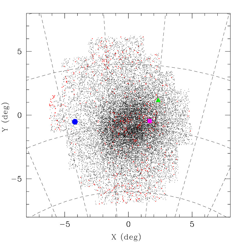
Figure 1: VMC coverage of the LMC. Black dots mark the $\sim 22,000$ RRLs analysed in this paper. Red dots are RRLs present in the $Gaia$ catalogue only. The centre of the map is $\alpha_{0}$=81.0 deg and $\delta_{0}$=$-$69.0 deg. The blue circle, magenta square and green triangle indicate the GCs NGC 2210, NGC 1835 and NGC 1786, respectively (see Section 4.3).

We cross-matched the VMC catalogue with the OGLE catalogue of RRLs in the LMC (Soszyński et al., 2016, 2019) and with the catalogue of confirmed LMC RRLs published as part of $Gaia$ DR2 (Clementini et al., 2019). We used $Gaia$ DR2 as the more recent eDR3 (Gaia Collaboration, Brown et al., 2020) does not contain an updated list of variable sources. This will become available with DR3 in 2022. The total number of OGLE RRLs in the VMC footprint is $\sim 35,000$, but in our analysis we considered only the OGLE fundamental-mode (RRab) and first-overtone pulsators (RRc): (i) for which both $V$ and $I$ light curves are available, (ii) without flags in the OGLE catalogue such as: uncertain, secondary period, possible Anomalous Cepheid, possible $\delta$ Scuti star, etc., and (iii) with a VMC counterpart found within 1 arcsec. Our total sample thus selected included 28,132 RRLs (21,152 RRab and 6,980 RRc). Furthermore, we cross-matched the Gaia catalogue of confirmed RRLs with the general catalogue of VMC sources in the LMC field of view. This allowed us to recover an additional 524 RRLs (357 RRab, and 167 RRc) which were missing in the OGLE catalogue of LMC RRLs. $Gaia$ has a smoother spatial sampling than OGLE thus allowing to recover additional RRLs in regions near to CCD edges and/or across inter-CCD gaps of the OGLE camera.

Figure 1 shows the spatial distribution of the full sample of RRLs analysed in this work. The X and Y coordinates are defined as in van der Marel & Cioni (2001) with $\alpha_{0}$=81.0 deg and $\delta_{0}$=$-$69.0 deg. Table 1 provides centre coordinates for the 68 VMC tiles covering the LMC and the number of RRLs contained in each tile.

Table 1: VMC tiles in the LMC analysed in the present study: (1) field and tile number; (2), (3) coordinates of the tile centre, J2000 epoch; (4) total number of RRLs in the tile, (5) extinction $E(V-I)$ and (6) absorption in the $K_{\mathrm{s}}$ band (see Section 3.3); (7) average period of the RRab stars in the tile and (8) dispersion of the average period of the RRab stars (see Section 2); (9), (10), (11), (12) and (13) coefficients of the $PL$ relations (in the form: $K_{\mathrm{s}_{0}}$=$a$ + $b$ $\times\log P$) for RRab and fundamentalised (by adding 0.127 to the logarithm of the first overtone period) RRc stars and their uncertainties (see Section 3.4).

Tile	R.A.	Dec	N	$\langle E(V-I)\rangle$	$\langle AK_{\mathrm{s}}\rangle$	$\langle Pab\rangle$	$\sigma_{\rm Pab}$	$a$	$b$	$\sigma_{a}$	$\sigma_{b}$	rms
	(h:m:s)	(∘:′:′′)		(mag)	(mag)	(d)	(d)	(mag)	(mag)	(mag)	(mag)
LMC 2_3	04:48:04	$-$74:54:11	84	0.121	0.035	0.577	0.067	17.45	$-$2.56	0.05	0.17	0.11
LMC 2_4	05:04:43	$-$75:04:45	111	0.134	0.039	0.586	0.061	17.50	$-$2.34	0.04	0.15	0.11
LMC 2_5	05:21:39	$-$75:10:50	125	0.158	0.046	0.575	0.066	17.44	$-$2.41	0.04	0.17	0.12
LMC 2_6	05:38:43	$-$75:12:21	107	0.128	0.037	0.596	0.082	17.38	$-$2.68	0.04	0.17	0.13
LMC 2_7	05:55:46	$-$75:09:17	82	0.145	0.042	0.577	0.066	17.43	$-$2.35	0.06	0.21	0.12
LMC 3_2	04:37:05	$-$73:14:30	114	0.105	0.031	0.594	0.064	17.46	$-$2.53	0.04	0.14	0.10
LMC 3_3	04:52:00	$-$73:28:09	170	0.111	0.032	0.587	0.069	17.43	$-$2.65	0.03	0.11	0.11
LMC 3_4	05:07:14	$-$73:37:50	216	0.127	0.037	0.580	0.063	17.45	$-$2.55	0.03	0.11	0.11
LMC 3_5	05:22:43	$-$73:43:25	250	0.121	0.035	0.589	0.072	17.42	$-$2.59	0.03	0.10	0.12
LMC 3_6	05:38:18	$-$73:44:51	218	0.133	0.038	0.578	0.064	17.42	$-$2.54	0.03	0.12	0.12
LMC 3_7	05:53:52	$-$73:42:06	160	0.115	0.033	0.579	0.082	17.45	$-$2.39	0.03	0.12	0.12
LMC 3_8	06:09:17	$-$73:35:12	138	0.118	0.034	0.573	0.059	17.38	$-$2.51	0.04	0.16	0.12
LMC 4_2	04:41:31	$-$71:49:16	232	0.139	0.040	0.581	0.062	17.46	$-$2.52	0.03	0.11	0.11
LMC 4_3	04:55:19	$-$72:01:53	311	0.110	0.032	0.584	0.068	17.45	$-$2.62	0.02	0.09	0.10
LMC 4_4	05:09:24	$-$72:10:50	485	0.080	0.023	0.578	0.067	17.47	$-$2.46	0.02	0.08	0.12
LMC 4_5	05:23:40	$-$-72:16:00	522	0.082	0.024	0.582	0.077	17.42	$-$2.60	0.02	0.07	0.12
LMC 4_6	05:38:00	$-$72:17:20	431	0.097	0.028	0.576	0.066	17.44	$-$2.46	0.02	0.09	0.13
LMC 4_7	05:52:20	$-$72:14:50	262	0.105	0.031	0.578	0.066	17.43	$-$2.43	0.03	0.11	0.12
LMC 4_8	06:06:33	$-$72:08:31	143	0.102	0.030	0.581	0.070	17.37	$-$2.67	0.04	0.14	0.11
LMC 4_9	06:20:33	$-$71:58:27	122	0.078	0.023	0.589	0.076	17.27	$-$2.90	0.04	0.15	0.12
LMC 5_1	04:32:44	$-$70:08:40	154	0.109	0.032	0.593	0.068	17.42	$-$2.71	0.03	0.10	0.10
LMC 5_2	04:45:19	$-$70:23:44	288	0.149	0.043	0.584	0.071	17.50	$-$2.35	0.03	0.10	0.12
LMC 5_3	04:58:12	$-$70:35:28	618	0.086	0.025	0.583	0.067	17.46	$-$2.57	0.02	0.07	0.13
LMC 5_4	05:11:17	$-$70:43:46	1138	0.082	0.02	0.582	0.069	17.44	$-$2.60	0.02	0.06	0.15
LMC 5_5	05:24:30	$-$70:48:34	1349	0.085	0.024	0.578	0.070	17.47	$-$2.42	0.02	0.06	0.16
LMC 5_6	05:37:48	$-$70:49:49	946	0.136	0.039	0.575	0.072	17.43	$-$2.52	0.02	0.08	0.17
LMC 5_7	05:51:05	$-$70:47:31	512	0.133	0.039	0.574	0.067	17.41	$-$2.53	0.02	0.09	0.14
LMC 5_8	06:04:16	$-$70:41:40	190	0.084	0.024	0.580	0.065	17.41	$-$2.48	0.03	0.10	0.11
LMC 5_9	06:17:18	$-$70:32:21	151	0.088	0.025	0.585	0.066	17.42	$-$2.43	0.03	0.12	0.10
LMC 6_1	04:36:49	$-$68:43:51	213	0.084	0.024	0.576	0.069	17.43	$-$2.59	0.03	0.11	0.13
LMC 6_2	04:48:39	$-$68:57:56	352	0.137	0.040	0.577	0.070	17.45	$-$2.54	0.03	0.09	0.13
LMC 6_3	05:00:42	$-$69:08:54	776	0.090	0.026	0.578	0.072	17.47	$-$2.53	0.02	0.08	0.17
LMC 6_4	05:12:56	$-$69:16:39	1305	0.094	0.027	0.581	0.074	17.47	$-$2.47	0.02	0.07	0.19
LMC 6_5	05:25:16	$-$69:21:08	1294	0.100	0.029	0.580	0.071	17.52	$-$2.35	0.02	0.07	0.20
LMC 6_6	05:37:40	$-$69:22:18	978	0.197	0.057	0.575	0.071	17.41	$-$2.68	0.02	0.08	0.18
LMC 6_7	05:50:03	$-$69:20:09	436	0.194	0.056	0.581	0.075	17.36	$-$2.64	0.02	0.09	0.14
LMC 6_8	06:02:21	$-$69:14:42	190	0.059	0.017	0.585	0.064	17.37	$-$2.55	0.03	0.11	0.11
LMC 6_9	06:14:33	$-$69:06:00	129	0.057	0.017	0.580	0.067	17.33	$-$2.54	0.03	0.12	0.10
LMC 6_10	06:26:32	$-$68:54:06	103	0.073	0.021	0.585	0.066	17.30	$-$2.68	0.04	0.14	0.10
LMC 7_1	04:40:09	$-$67:18:20	125	0.070	0.020	0.585	0.077	17.45	$-$2.52	0.04	0.15	0.12
LMC 7_2	04:51:35	$-$67:31:57	291	0.097	0.028	0.584	0.072	17.44	$-$2.57	0.03	0.10	0.13
LMC 7_3	05:02:55	$-$67:42:15	477	0.089	0.026	0.572	0.072	17.43	$-$2.62	0.02	0.08	0.14
LMC 7_4	05:14:24	$-$67:49:31	749	0.102	0.030	0.577	0.072	17.47	$-$2.43	0.02	0.07	0.14
LMC 7_5	05:25:58	$-$67:53:42	709	0.137	0.040	0.579	0.073	17.44	$-$2.50	0.02	0.07	0.13
LMC 7_6	05:37:35	$-$67:54:47	440	0.116	0.034	0.582	0.069	17.42	$-$2.46	0.02	0.08	0.13
LMC 7_7	05:49:12	$-$67:52:45	265	0.113	0.033	0.581	0.064	17.35	$-$2.57	0.03	0.10	0.12
LMC 7_8	06:00:45	$-$67:47:38	162	0.056	0.016	0.598	0.074	17.38	$-$2.38	0.03	0.11	0.11
LMC 7_9	06:12:12	$-$67:39:26	100	0.051	0.015	0.579	0.075	17.32	$-$2.65	0.03	0.12	0.10
LMC 7_10	06:23:29	$-$67:28:15	48	0.061	0.018	0.599	0.078	17.40	$-$2.23	0.06	0.22	0.11
LMC 8_2	04:54:12	$-$66:05:48	186	0.104	0.030	0.593	0.071	17.43	$-$2.58	0.03	0.12	0.12
LMC 8_3	05:04:54	$-$66:15:30	238	0.071	0.020	0.580	0.071	17.38	$-$2.62	0.03	0.12	0.13
LMC 8_4	05:15:43	$-$66:22:20	301	0.095	0.028	0.582	0.071	17.42	$-$2.45	0.03	0.10	0.13
LMC 8_5	05:26:38	$-$66:26:16	287	0.086	0.025	0.585	0.075	17.38	$-$2.56	0.03	0.10	0.12
LMC 8_6	05:37:34	$-$66:27:16	255	0.082	0.024	0.586	0.067	17.37	$-$2.50	0.03	0.11	0.13
LMC 8_7	05:48:30	$-$66:25:20	172	0.073	0.021	0.575	0.066	17.34	$-$2.54	0.04	0.14	0.13
LMC 8_8	05:59:23	$-$66:20:29	145	0.040	0.012	0.596	0.077	17.36	$-$2.52	0.03	0.11	0.10
LMC 8_9	06:10:11	$-$66:12:44	101	0.062	0.018	0.582	0.071	17.30	$-$2.54	0.04	0.16	0.11
LMC 9_3	05:06:41	$-$64:48:40	111	0.052	0.015	0.594	0.067	17.45	$-$2.30	0.04	0.15	0.12
LMC 9_4	05:16:55	$-$64:55:08	178	0.061	0.018	0.581	0.067	17.38	$-$2.46	0.03	0.11	0.11
LMC 9_5	05:27:14	$-$64:58:49	209	0.072	0.021	0.582	0.063	17.38	$-$2.40	0.03	0.10	0.11
LMC 9_6	05:37:35	$-$64:59:44	163	0.059	0.017	0.582	0.063	17.28	$-$2.67	0.03	0.12	0.11
LMC 9_7	05:47:55	$-$64:57:53	117	0.068	0.020	0.589	0.065	17.35	$-$2.37	0.04	0.14	0.11
LMC 9_8	05:58:13	$-$64:53:15	114	0.047	0.014	0.588	0.071	17.31	$-$2.49	0.04	0.14	0.10
LMC 9_9	06:08:26	$-$64:45:53	61	0.083	0.024	0.568	0.062	17.23	$-$2.81	0.06	0.20	0.12
LMC 10_4	05:18:01	$-$63:27:54	107	0.045	0.013	0.583	0.070	17.37	$-$2.49	0.03	0.12	0.09
LMC 10_5	05:27:49	$-$63:31:23	116	0.061	0.018	0.587	0.065	17.33	$-$2.59	0.04	0.14	0.11
LMC 10_6	05:37:38	$-$63:32:13	105	0.077	0.022	0.585	0.066	17.36	$-$2.38	0.04	0.14	0.11
LMC 10_7	05:47:26	$-$63:30:25	91	0.050	0.015	0.581	0.070	17.32	$-$2.53	0.05	0.19	0.12

Time-series $Y$, $J$ and $K_{\mathrm{s}}$ photometry for the RRLs observed by the VMC survey is provided in Table 2. The table contains the Heliocentric Julian Date (HJD) of the observations inferred from the VSA (column 1), the $Y$, $J$ and $K_{\mathrm{s}}$ magnitudes obtained using an aperture photometry diameter of 2.0 arcsec (column 2), and the error on the magnitudes (column 3). The light curves contain only epoch data observed within pre-defined constraints, that is with conditions of seeing $<1^{\prime\prime}$ for $K_{\mathrm{s}}$, $<1.2^{\prime\prime}$ for $Y$ and, $<1.1^{\prime\prime}$ for $J$, airmass $<$1.7 and moon distance $>70^{o}$ (Cioni et al., 2011). The full catalogue of light curves is available in the electronic version of the paper.

Table 2: $Y$, $J$ and $K_{\mathrm{s}}$ time-series photometry for the RRLs analysed in this paper. The table is published in its entirety as Supporting Information with the electronic version of the article. A portion is shown here for guidance regarding its format and content.

VMC-558396536162
HJD$-$2400000	$Y$	errY
55583.680443	18.24	0.02
55597.606813	18.42	0.03
55878.818319	18.39	0.03
55983.600130	18.30	0.02
56004.513472	18.51	0.03
HJD$-$2400000	$J$	errJ
55589.666983	18.07	0.02
55615.569205	18.13	0.03
55980.563227	18.10	0.03
56004.533138	18.22	0.04
HJD$-$2400000	$K_{\mathrm{s}}$	errKs
55979.576519	17.73	0.05
55980.586298	17.78	0.08
55981.562849	17.71	0.05
55983.620398	17.78	0.07
55986.562678	17.83	0.06
55992.575373	17.80	0.07
56009.519064	17.76	0.07
56178.854539	17.78	0.05
56197.794262	17.86	0.06
56214.835096	17.89	0.06
56232.750233	17.77	0.05
56232.792530	17.76	0.05
56255.668172	17.89	0.06
57044.537788	18.05	0.13

The $K_{\mathrm{s}}$ photometry of the VISTA system is tied to the Two Micron All Sky Survey (2MASS; Skrutskie et al. 2006) photometry. The complete set of transformation relations from one system to the other is available on the CASU web site or in the work by Gonzalez-Fernandez et al. (2018). We used the photometry in the VISTA system v1.5. The periods provided by the OGLE catalogue were used to fold the $Y,J$ and $K_{\mathrm{s}}$ light curves of the RRLs observed by OGLE, whereas we used the periods provided in the Gaia DR2 RRL vari_table for the sources observed only by Gaia as the eDR3 release does not contain update information for variable stars like period, epoch of maximum light and photometry. Examples of the $Y$, $J$ and $K_{\mathrm{s}}$ light curves for an RRab and an RRc star are shown in Figure 2. A complete atlas of light curves is provided in electronic form. The $K_{\mathrm{s}}$ light curves are very well sampled, with on average, 13–14 sampling points, confirming the soundness of the VMC observing strategy for RRLs. Typical errors for the individual $K_{\mathrm{s}}$ data points are in the range of 0.06 – 0.1 mag. The light curves in the $Y$ and $J$ bands have on average four phase points. Average errors for the individual $Y$ and $J$ observations are 0.03 and 0.04 mag, respectively.

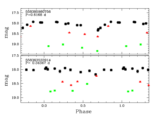
Figure 2: $Y$ (green squares), $J$ (red triangles) and $K_{\mathrm{s}}$ (black dots) light curves for an RRab (top panel) and an RRc (bottom panel) star in the LMC field. The VMC ID and the period are provided in the top left-hand corner. Typical errors for individual $K_{\mathrm{s}}$ epochs are about 0.06 mag and 0.1 mag for RRab and RRc stars, respectively. For $Y$- and $J$-bands typical errors are 0.03 and 0.07 mag for RRab and RRc stars, respectively.

Table 3: List of LMC RRLs analysed in the paper: OGLE IV ID (5 digit number $-$OGLE-LMC-RRLYR-) or Gaia DR2 ID ($>$9 digit number) column (1), VMC ID is column (2), J2000 coordinates R.A. and Dec. from the VMC catalog are columns (3) and (4), pulsation mode (column 5), period (column 6) and epoch of maximum light ($-$2456000 for OGLE sources, $-$ 2455197.5 for Gaia DR2 sources) column (7), metallicity is column (8), absorption in the $K_{\mathrm{s}}$-band (column 9), number of epochs in the $K_{\mathrm{s}}$-band (column 10), Y (column 11) and J band (column 12), columns (13), (14), and (15) are average VMC magnitudes: $\langle Y\rangle$, $\langle J\rangle$ and $\langle K_{\mathrm{s}}\rangle$. The table is published in its entirety as Supporting Information with the electronic version of the article. A portion is shown here for guidance regarding its form and content.

ID	ID(VMC)	R.A.	Dec.	Type	$P$	$T_{0}$	[Fe/H]	$A_{K_{\mathrm{s}}}$	$N_{K_{\mathrm{s}}}$	$N_{Y}$	$N_{J}$	$\langle K_{\mathrm{s}}\rangle$	$\langle Y\rangle$	$\langle J\rangle$
		deg	deg		(d)	(d)	dex	(mag)				(mag)	(mag)	(mag)
34314	558346514686	84.202208	–74.490389	ab	0.7040914	0.46883		0.028	26	8	8	18.12	18.64	18.50
33596	558346517950	82.979042	–74.501333	ab	0.6610381	0.29199	$-$1.424	0.035	13	4	4	17.94	18.39	18.21
35139	558346518034	85.807625	–74.498722	ab	0.4889976	0.25714	$-$1.592	0.036	13	4	4	18.20	18.88	18.66
34860	558346519807	85.190208	–74.510083	c	0.3114614	0.24308	$-$1.507	0.082	13	4	4	18.45	18.88	18.77
34267	558346526561	84.127458	–74.540444	ab	0.53476	0.08816		0.037	13	4	4	18.10	18.53	18.32
34756	558346526744	85.008125	–74.538944	ab	0.55045	0.16538		0.082	12	3	4	17.95	18.37	18.25
34635	558346527385	84.747875	–74.543194	c	0.34962	0.01419	$-$1.527	0.043	13	4	4	18.41	18.82	18.60

3 Period–Luminosity and Period–Wesenheit relations

3.1 Average NIR magnitudes

Mean $Y,J$ and $K_{\mathrm{s}}$ magnitudes for the LMC RRLs were derived as a simple mean of magnitudes expressed in flux units, without modelling the light curves.

For RRLs observed in the optical, integrating the modelled light curve over the whole pulsation cycle is the correct procedure to derive the mean magnitude. However, in the NIR, amplitudes are so small that the difference between intensity-averaged mean magnitudes of the modelled light curves and the simple mean of the magnitudes in flux units is negligible. A comparison of the two mean values, where the former were computed by modelling the light curves with a Fourier series using the Graphical Analyzer of Time Series package (GRaTIS; custom software developed at the Bologna Observatory by P. Montegriffo, see e.g. Clementini et al. 2000), for a sample of 170 LMC RRLs showed that the differences between the two procedures are less than 0.02 mag, that is, smaller than the average errors of the two methods. Table 3 lists the $Y$, $J$ and $K_{\mathrm{s}}$ mean magnitudes obtained as simple means of the magnitudes (in flux units) along with the main properties of the stars, namely, OGLE IV or Gaia DR2 ID, period, pulsation mode, epoch of maximum light, VMC ID and number of observations in the $K_{\mathrm{s}}$, $Y$ and $J$ bands.

The average magnitudes were used to place the RRLs in the $J-K_{\mathrm{s}}$ vs $K_{\mathrm{s}}$ CMD, shown in Figure 3. The RRLs are marked with small green dots.

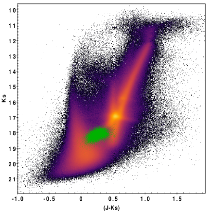
Figure 3: CMD of all VMC sources matching the Gaia eDR3 catalogue using the criteria defined in the text. A total of  6.9 million sources are shown in this diagram. The RRLs analysed in this paper are marked by small green dots.

To construct the CMD we selected from the Gaia eDR3 catalogue (Gaia Collaboration, Brown et al., 2020) an area of 8.8 degrees in radius around the centre of the LMC ($\alpha_{0}$=80.8 deg, $\delta_{0}$=$-$69.7 deg) which contained more than 25 million objects. We chose this area in order to fully cover the LMC regions tiled by the VMC observations as well as the whole footprint of the OGLE-IV survey. We assumed as bona fide LMC members only sources in the selected area with parallaxes ($\varpi$) and proper motions ($\mu_{\alpha}^{*},\mu_{\delta}$) satisfying the following criterion:

$$\begin{split}\sqrt{(}(\varpi-\varpi_{\rm LMC})^{2}+(\mu_{\alpha}^{*}-{\mu_{\alpha}^{*}}_{\rm LMC})^{2}+\\ (\mu_{\delta}-{\mu_{\delta}}_{\rm LMC})^{2})<1,\end{split}$$ (1)

where $\varpi_{\rm LMC}=-0.0040\pm 0.3346$ mas , ${\mu_{\alpha}^{*}}_{\rm LMC}=1.7608\pm 0.4472$ mas yr^-1 and ${\mu_{\delta}}_{\rm LMC}=0.3038\pm 0.6375$ mas yr^-1 are the mean LMC parallax and proper motions from Gaia Collaboration et al. (2020c). We then cross-matched the sources satisfying the above condition with the VMC general catalogue, thus obtaining a final sample of $\sim 6.9\times 10^{6}$ sources shown in Figure 3. The proper motions and parallaxes of the CMD stars are from $Gaia$ eDR3 which contains the most recent and accurate astrometry and photometry available from $Gaia$.

Figure 4: K_s band absorption map derived from the RRab stars. The position of each RRL was re-binned to a circle of 30 arcsec in diameter.

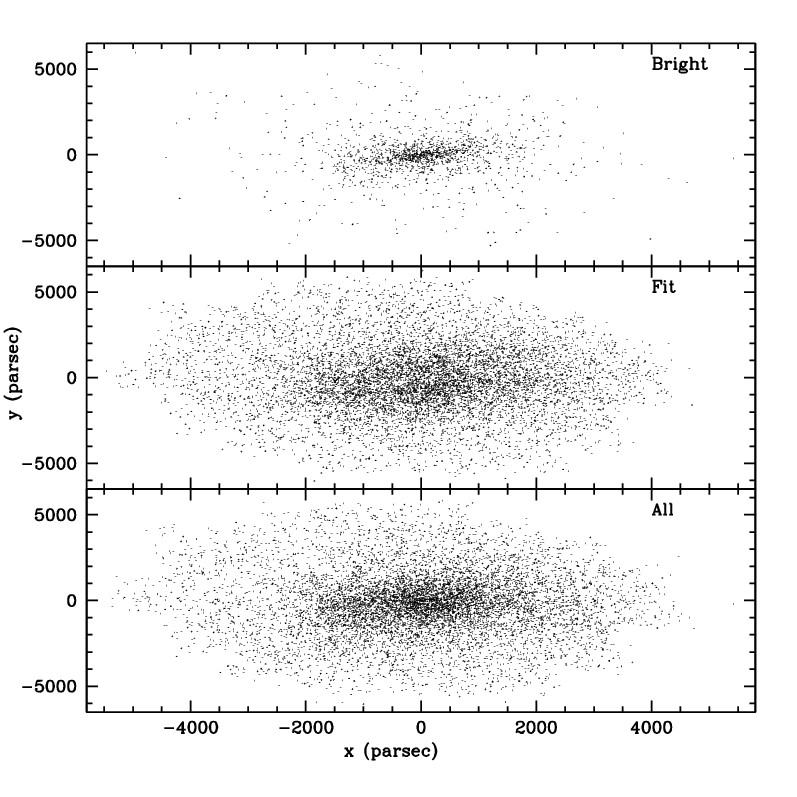
Figure 5: Bottom: Spatial distribution of the whole sample of RRLs ($\sim 29,000$) considered in the paper; Middle: distribution of the RRLs which were actually used to fit the $PL_{K_{\mathrm{s}}}$ relation ($\sim 22,000$); Top: distribution of the RRLs which appear to be overluminous in the $PL_{K_{\mathrm{s}}}$ relation ($\sim 7,000$), hence were discarded. They are mainly located along the LMC bar, thus explaining the gap seen in that region in the middle panel.

3.2 Reddening from the RR Lyrae stars

For each RRL pulsating in the fundamental mode a reddening estimate was obtained using the relation derived by Piersimoni et al. (2002) which provides the intrinsic $V-I$ colour of fundamental-mode RRLs as a function of the star’s period and amplitude in the $V$ band:

$${(V-I)_{0}=0.65(\pm 0.02)-0.07(\pm 0.01){\rm AmpV}+}$$

$${+0.36(\pm 0.06)\log P~{}~{}~{}~{}~{}~{}\sigma=0.02}.$$ (2)

where periods and amplitudes (in the $I$-band) for the RRLs were taken from the OGLE IV catalogue (Soszyński et al., 2016), and the $I$-band amplitudes were transformed to $V$-band amplitudes by adopting a fixed amplitude scaling factor of AmpV$/$AmpI=1.58. This value was derived from a statistically significant (75) data set of RRLs in Galactic GCs (see Di Criscienzo et al. 2011). The intrinsic $V-I$ colours were then used to derive individual $E(V-I)$ reddening values for each RRL. These $E(V-I)$ values were then converted to extinction in the $Y$, $J$ and $K_{\mathrm{s}}$ passbands using the coefficients : $A_{Y}$ = 0.385A_V, $A_{J}$ = 0.283$A_{V}$, and $A_{K}$ = 0.114A_V with $A_{V}$= 2.4$E(V-I)$ from Kerber et al. (2009), which were derived from the Cardelli et al. (1989) extinction curve. The RRL absorption map in the K_s band derived from the RRab stars is shown in Figure 4. This map was used to estimate by interpolation the absorption for the RRLs in the $Gaia$ sample which lack $V$ and $I$ magnitudes and for the RRc stars for which Equation 3.2 is not applicable. The complete set of $A_{K_{\mathrm{s}}}$ values is given in the ninth column of table 3. It is interesting to note how the most active star forming regions in the LMC like 30 Doradus pop up in the map. All over the LMC the average extinction is small and its value in the $K_{\mathrm{s}}$ band is: $A_{K_{\mathrm{s}}}$=0.03 mag with $\sigma=0.02$ mag. A comparison of the reddening values derived from RC stars (Tatton et al., 2013) and the values estimated from RRLs using the Piersimoni et al. (2002) formula shows that there is a qualitative agreement between the two methods. However, this agreement should be taken with some caution as Tatton et al. (2013)’s work is based on stars in a limited area of the LMC, surrounding the 30 Doradus region. Indeed, substantial differences between the reddening maps derived from RCs, background galaxies and RRLs were found for example in the SMC by Bell et al. (2020). These differences most likely arise from RCs, RRLs and background galaxies sampling regions at different depths. In fact, RCs are expected to be embedded in the dust layers, RRLs probably are half in front and half in the background, and galaxies are definitely in the far field. One can thus expect some spatial correlations in the mean extinction values, but not identical values from these different indicators.

3.3 Blended sources

Our first attempt to derive the $PL_{K_{\mathrm{s}}}$ relation has revealed a number of RRLs brighter than the main relation. We investigated their spatial distribution and found that they are mainly located in the central part of the LMC. This is shown in Figure 5 which presents in the bottom panel the spatial distribution of the whole sample of RRLs considered in this paper ($\sim 29,000$), in the top panel the distribution of the RRLs which appear to be overluminous in the $PL_{K_{\mathrm{s}}}$ relation and, in the middle panel, the distribution of the RRLs which were actually used to fit our final $PL_{K_{\mathrm{s}}}$ relation. Further investigations, performed using the Fourier parameters ($\phi_{31},\phi_{21},R_{21}$ and $R_{31}$) of the light curves available in the OGLE IV catalogue did not show any particular properties of the overluminous RRLs. On the other hand, in the period–amplitude diagram based on the $I$ amplitudes available in the OGLE IV catalogue, the bright RRLs all show small, in some cases near-zero amplitudes, compared with regular RRLs of the same period. The decrease in amplitude at a given period can be owing to these RRLs being blended with non-variable stars. We expect the centroid of a blended source to be determined with poor accuracy (see e.g. Ripepi et al., 2014, 2015). For this reason as a further test we plotted the distribution of distances in arcsec of the VMC sources cross-matched with the OGLE IV RRLs. A clear separation is now seen in the two samples, for 94% of the RRLs lying on the $PL/PW$ relations the cross-match radius is less than 0.2 arcsec, whereas for 68% of the overluminous RRLs the cross-match radius is larger than 0.2 arcsec. The average accuracy of the VMC astrometry is on the order of 0.080 arcsec both in R.A. and in Dec. (Cioni et al., 2011). We therefore discarded the RRLs with a cross-match radius larger than 0.2 arcsec. A total of 3252 objects were discarded. This procedure allowed us to significantly reduce the scatter on the $PL/PW$ relations. We visually inspected the VMC images of some of the discarded RRLs, confirming that they all are clearly blended with stars and/or background galaxies. Similar investigations were performed in the past and the same effects were noted, e.g. by Ripepi et al. (2015) for Type II Cepheids. The final sample of LMC RRLs after this cleaning procedure contains 25,795 objects. This is the sample that was used as a starting point to investigate the $PL$ and $PW$ relations presented in the following sections. Additional RRLs were later discarded from the final fit based on a 3-$\sigma$ clipping procedure leading to $PL_{K_{\mathrm{s}}}$ relations using a clean sample of $\sim 22,000$ RRLs.

3.4 Metallicity of the RR Lyrae stars

Knowledge of the metallicity ($Z$) is needed to construct $PLZ$ and $PWZ$ relations for RRLs. However, spectroscopic metallicities are available only for a very limited number of LMC RRLs (e.g. Gratton et al. 2004; Borissova et al. 2004, 2006 and references therein). Jurcsik & Kovács (1996) and Morgan et al. (2007) showed that it is possible to derive a “photometric” estimate of the metal abundance ([Fe/H]) of an RRL of known pulsation period from the $\phi_{31}$ Fourier parameter of the $V$-band light curve decomposition. A new calibration of the $\phi_{31}$–[Fe/H] relation for fundamental-mode and first-overtone RRLs was published by Nemec et al. (2013), based on excellent accuracy RRL light curves obtained with the Kepler space telescope, and metallicities derived from high resolution spectroscopy. This new calibration provides metal abundances directly tied to the metallicity scale of Carretta et al. (2009) which is based on high dispersion spectroscopy and holds for the metallicity range from [Fe/H]$\sim$ 0.0 to $\sim-$2.6 dex.

Skowron et al. (2016) applied the calibration of Nemec et al. (2013) to the OGLE-IV fundamental mode RRLs, obtaining a median metallicity value of [Fe/H]=$-1.59\pm 0.31$ dex for the LMC on the Zinn & West (1984) scale. Metallicities from Skowron et al. (2016) are available for 16,570 LMC RRab stars in our sample. This sample was used to compute a metallicity map of the LMC. Through the interpolation of this map it was possible to give a metallicity estimate also to the RRc stars. The single [Fe/H] values in Skowron et al. (2016) and the ones derived from the metallicity map, were used to compute the metallicity-dependent relations listed in Tables 4 and 5. A non-linear least-squares Marquardt–Levenberg algorithm (e.g. Mighell 1999) was used to fit the $PLZ$ and $PWZ$ relations along with a 3 $\sigma$ clipping procedure to clean from outliers. Our final $PLZ$ and $PWZ$ relations are based on a sample $\sim 13,000$ RRab and $\sim 5,000$ RRc stars (see Tables 4 and 5).

3.5 Derivation of the $PL(Z)$ and $PW(Z)$ relations

$PL_{K_{\mathrm{s}}}$(Z) relations were computed using the periods, $\langle K_{\mathrm{s}}\rangle$ mean magnitudes, absorption values and metallicity for the RRLs listed in Table 3. We fitted a linear least-squares relation of the form: $m_{X0}=a+b\times\log P+c\times$[Fe/H]. For the global relation (Glob), which includes RRab plus RRc stars, the periods of the RRc stars were fundamentalised using the classical relation $\log P_{FU}{\rm(RRc)}$ = $\log P_{\rm RRc}$ + 0.127 (Iben, 1974). Only stars with $E(V-I)>0$ mag were considered and an unweighted least-squares fit with 3 $\sigma$ clipping was applied, hence reducing the sample of RRLs actually used to construct the $PL$ relations to around 22,100 sources ($\sim$16,900 RRab and $\sim$5,200 RRc). The same procedure was used to obtain $PL$ relations in the $Y$ and $J$ bands. There are on average only 3–4 phase points for each RRL in the VMC data available in the $Y$ and $J$ bands (see Table 2). Hence, the resulting average magnitudes have larger errors and the $PL$ relations in $Y$ and $J$ have larger rms values than for the $K_{\mathrm{s}}$  band. In the optical we obtained a $PL$ relation in the $I$ band using the OGLE IV data. The $PL$ and $PLZ$ relations derived using this procedure are summarised in Table 4. In the case of the $PL_{K_{\mathrm{s}}}$ we also derived individual relations for each VMC tile and their parameters are given in Table 1. Figure 6 shows the $PL$ relations in the $I$, $Y$, $J$ and ${K_{\mathrm{s}}}$ bands obtained for RRab (FU), RRc (FO) on the left and for RRab plus fundamentalised RRc stars (Glob) on the right.

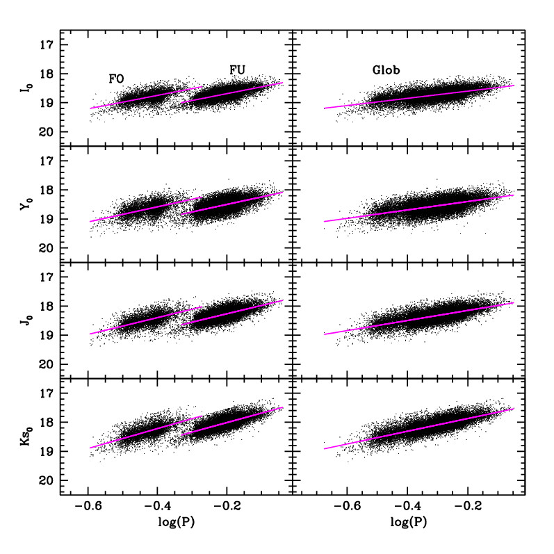
Figure 6: De-reddened mean magnitudes versus $\log P$, for RRLs in the LMC. Black points are stars retained for the final $PL$ computation. The left-hand panels show RRc (first overtone, FO) and RRab stars (fundamental mode, FU) separately. The right-hand panels show all RRLs after the $\log P$ of the RRc stars was fundamentalised. The magenta lines show the $PL$ relations derived using these data (see Table 4).

Reddening-independent $PW$ relations can be obtained by combining magnitudes and colours in different bands. These reddening free magnitudes were introduced by Madore & van den Bergh (1975) and Madore (1982). They are defined as: $W(X,Y)=m_{X}$ – $R(m_{Y}$–$m_{X}$) where $X$ and $Y$ are two different passbands and $R$ is the ratio between selective absorption in the $X$ band and colour excess in the adopted colour. These coefficients are fixed according to the Cardelli et al. (1989) law. A set of $PW$ and $PWZ$ relations was obtained fitting the VMC $Y$, $J$ and $K_{\mathrm{s}}$ and OGLE IV $V$, $I$ photometry to the equation $m_{X}-R\times(m_{Y}-m_{X})=a+b\times\log P+c\times$[Fe/H]. The parameters obtained are summarised in Table 5. The PW relations in different bands are presented in Figure 7.

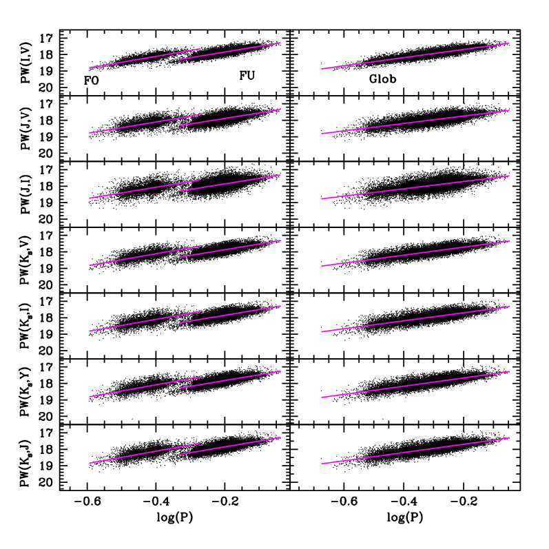
Figure 7: As in Figure 6 but for Wesenheit magnitudes. The magenta lines show the $PW$ relations presented in Table 5.

3.6 Gaia Proper Motions for the LMC RR Lyrae stars

The recently released Gaia eDR3 catalogue (Gaia Collaboration, Brown et al., 2020) includes proper motions for 21,801 RRLs in our catalogue, with average errors of $\sigma_{\mu_{\alpha}^{*}}\sim 0.30$ and $\sigma_{\mu_{\delta}}\sim 0.32$ mas yr^-1, respectively. We selected RRL stars in the LMC retaining only sources with proper motions within 1$\sigma$ from the average proper motions in R.A. and Dec. of the whole sample of 21,801 RRLs, that are $\langle{\mu_{\alpha}^{*}}\rangle=1.85$ and $\langle{\mu_{\delta}}\rangle=0.36$ mas yr^-1, respectively. This resulted in a subsample of 4690 RRLs. A fit of the PL_Ks relation using only this Gaia proper motion-selected sample of RRLs provides: $a$= 17.44 mag, $b=-$2.55 mag, $\sigma_{a}=0.01$ mag, $\sigma_{b}=0.03$ mag, rms= 0.14. This is consistent with the global relation (Glob) presented in Table 4. A similar analysis was performed for the other PL(Z) and PW(Z) relations presented in table 4 and 5 obtaining always consistent results. This gives us confidence that the $PL$ and $PW$ relations derived in this paper are based on samples of RRLs which are bona fide LMC members.

3.7 Comparison with theory and other papers

As a final step of our analysis of the RRL $PL$ relations we have compared the $PLZ$ and $PWZ$ relations obtained here with the theoretical results of Marconi et al. (2015).

Three of our $PLZ$ and six of our $PWZ$ relations have a counterpart in Marconi et al. (2015). A comparison of the matching relations shows that the slopes in period and metallicity are different, with an average difference of 0.53($\pm 0.05$) dex units in the $\log P$ term and 0.07($\pm 0.01$) dex units in the metallicity term. This is clearly seen in Figure 8 where the parameters of some PWZ relations derived in this work are compared with those in the corresponding relations by Marconi et al. (2015).

These differences most likely arise from the larger dependence on metallicity of the theoretical relations, which predict metallicity terms on the order of 0.2 mag dex^-1. Further comparisons with the theoretical pulsation scenario will be discussed in a future paper (M. I. Moretti et al., in preparation). Such a large metallicity dependence is not observed for several empirical RRL $PLZ$ relations in the literature (e.g. Del Principe et al., 2006; Sollima et al., 2008; Borissova et al., 2009). However, using literature data for Milky Way (MW) field RRLs, Muraveva et al. (2018a) derived an empirical absolute $PLZ(K)$ relation calibrated using Gaia DR2 parallaxes, which shows a non-negligible dependence on metallicity, in the same direction as that found by the theoretical $PLZ$ relations. Similarly, Sesar et al. (2017b) and then Neeley et al. (2019) using Gaia DR2 parallaxes found for the metallicity slopes of the PLZ relations values between 0.17 and 0.20 mag dex^-1. A possible explanation for the differences in the metallicity term (and, in turn, also for the $\log P$ term) is that the RRLs considered by the Marconi et al. (2015), Muraveva et al. (2018a), Neeley et al. (2019) and Sesar et al. (2017b) span a range in metallicity from $Z$ = 0.0001 to $Z$ = 0.02, while the metallicity of the LMC RRLs covers a much smaller range from $Z$=0.0001 to $Z$=0.001 (Carrera et al., 2008), hence lacking the more metal-rich component observed in the MW. A comparison between the coefficients of the PLZ relations for RRab + fundamentalised RRc stars derived in this paper and in those cited above is shown in Figure 9. The fit parameters differences range from an almost consistency in 1 $\sigma$ in the $J$ band b parameters to a 6 $\sigma$ difference for c parameters in the same band. Consistently larger differences arise in the $Y$,$J$ and $K_{\mathrm{s}}$ bands for the c parameters. While for the b parameters the largest difference are seen especially for the $K_{\mathrm{s}}$ band.

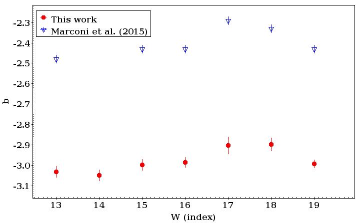
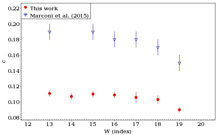
Figure 8: Comparison of the coefficients of the PWZ relations for RRab stars derived in this paper with those of the corresponding relations of Marconi et al. (2015). In the left-hand panel are shown the period slopes, while the right-hand panel shows the metallicty slopes. The $W$ indices are labelled as follows: $13=PW(K_{\mathrm{s}},J),14=PW(K_{\mathrm{s}},Y),15=PW(K_{\mathrm{s}},I),16=PW(K_{\mathrm{s}},V),17=PW(J,I),18=PW(J,V)$ and $19=PW(I,V)$.

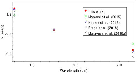
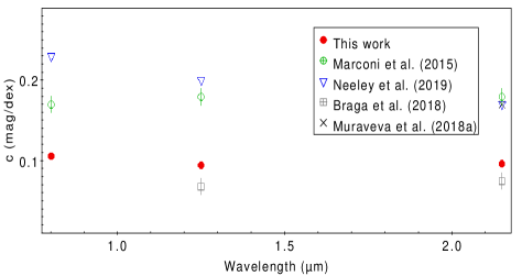
Figure 9: Comparison of the coefficients of the PLZ relations for RRab + fundamentalised RRc stars derived in this paper with those indicated in the legend. The period slopes are shown in the left-hand panel and the metallicity slopes in the right-hand panel. The errors of Neeley et al. (2019) and Muraveva et al. (2018a) are not reported to avoid confusion.

4 Structure of the LMC

4.1 Individual distances to RR Lyrae stars

The $PL$ and $PW$ relations derived in the previous sections can be used to infer the distance to each RRL in our LMC sample once a zero point is adopted. For this analysis we do not rely on the PLZ relations as they are based on a smaller sample than the PL relationships. We assumed as distance to the LMC centre the estimate of Pietrzyński et al. (2013) which corresponds to $d_{0}=49.97\pm 1.12$ kpc or to a distance modulus of $(m-M)_{0}$ =18.49 mag. However, this choice does not affect our study of the LMC’s structure, for which we rely on differential distances.

We measured the distance to each RRL using the $PL_{K_{\mathrm{s}}}$ relation and two different versions of the $PWZ$s. Results obtained from the three different relations were then compared. Since the $PWZ$s include a metallicity term, their application is limited to the RRab and RRc sample for which we have metallicities. We chose to adopt the $K_{\mathrm{s}}$, $J-K_{\mathrm{s}}$ and the $K_{\mathrm{s}}$, $V-K_{\mathrm{s}}$ $PWZ$ relations. We adopted the former because the $K_{\mathrm{s}}$ and $J$ bands are less sensitive to possible deviations from the colour correction, and the latter because it is weakly dependent on the colour term ($R$=0.13). We opted for the $PL_{K_{\mathrm{s}}}$ relation because it is less affected by reddening, and used the global version, which allowed us to determine the distances to 22,122 RRLs of both RRab and RRc types. The average error in the distance estimate for each RRL is of the order of $\sim 3.5$ kpc ( $\sim 0.15$ mag). The mean difference between the distances measured using the two $PWZ$ relations is 0.45 pc, whereas the mean difference between distances from the $PW(K_{\mathrm{s}}$, $V-K_{\mathrm{s}}$) and the $PL_{K_{\mathrm{s}}}$ relations is 23 pc ($\sim 0.001$ mag), which is very small compared with the average individual error of each RRL. In the following analysis we rely on the distances derived using the $PL_{K_{\mathrm{s}}}$ since it is based on a larger sample of RRLs, it has the smaller rms between the PL relations derived here and the ${K_{\mathrm{s}}}$ band is the one that is less effect by reddening.

4.2 3-D geometry of the LMC

Once the distance to each RRL is determined, it is possible to derive the Cartesian distribution of the RRLs from the R.A., Dec coordinates and the individual distances using the method described by van der Marel & Cioni (2001) and Weinberg & Nikolaev (2001):

$$x =-d~{}{\rm sin}(\alpha-\alpha_{0}){\rm cos}\delta$$

$$y =d~{}{\rm sin}\delta{\rm cos}\delta_{0}-d~{}{\rm sin}\delta_{0}{\rm cos}(\alpha-\alpha_{0}){\rm cos}\delta$$ (3)

$$z =d_{0}-d~{}{\rm sin}\delta{\rm sin}\delta_{0}-d~{}{\rm cos}\delta_{0}{\rm cos}(\alpha-\alpha_{0}){\rm cos}\delta,$$

where $d$ is the individual distance to each RRL, $d_{0}$ is the distance to the LMC centre and ($\alpha_{0}$, $\delta_{0}$) are the R.A. and Dec. coordinates of the LMC centre. We assume as reference system ($x,y,z$) one that has the origin in the LMC centre at ($\alpha_{0},\delta_{0}$ and $d_{0}$), the $x$-axis anti-parallel to the R.A.-axis, the $y$-axis parallel to the Dec. axis and the $z$-axis pointing towards the observer. The $\alpha_{0}$, $\delta_{0}$ coordinates of the LMC centre were derived from the average position of the RRLs ($\alpha_{0}=80^{\circ}.6147,\delta_{0}=-69^{\circ}.5799$). Our centre is offset by $\sim 0.8^{\circ}$ from the LMC centre of El Youssoufi et al. (2019, $\alpha_{0}=81^{\circ}.24,\delta_{0}=-69^{\circ}.73$), which was obtained using stellar density maps of all the stellar populations in the LMC.

As a first approach we divided the LMC into ($x,y$) planes by considering different intervals in distance. Figure 10 shows the distribution of the LMC RRLs in Cartesian coordinates divided into bins of distance. The bins were of the same order as the average distance standard deviation, $\sim 3.5$ kpc. Going clockwise from the top right-hand panel the RRLs are mapped for increasing distance values. A quick look shows that there are two extreme cases, with the RRLs closest (top right-hand panel) and most distant to us (top left-hand panel) showing different spatial distributions. A fraction of the RRLs in the top right-hand panel of Figure 10 appear to be spread all over the field and are likely RRLs belonging to the MW halo. This view is corroborated by the proper motions of the RRLs in this sample of which 43% are outside of 1 $\sigma$ the average $\mu_{\alpha}^{*}$ and $\mu_{\delta}$ values. These stars are placed mainly in the central region of this plot. On the other hand, it is also possible that this sample of RRLs belong to the outer most region of the elongated LMC halo, which is distorted by tidal forces owing to the interaction with the MW. This would explain why the proper motions are different from the average values in the main body of the LMC. In the same direction El Youssoufi et al. (submitted, see sect. 2.3) finds that the centre of the stellar proper motions for stars in the outer regions of the SMC is shifted from that of the inner regions, suggesting that these stars are probably associated to the LMC. In the same sample a concentration of RRLs likely belonging to the LMC shows up right and south of the centre. That is the part of the LMC which points towards the MW. The average coordinates of the RRLs in this panel are $\langle(x,y)\rangle=(-309,241)$ pc and they represent 5.1% of the whole sample. In the middle right-hand panel are shown RRLs with distances between 44 and 47 kpc and it is still possible to notice a protrusion of stars in the same region as in the previous panel. The centre coordinates in this case are $\langle(x,y)\rangle=(-667,491)$ pc, for 12.5% of RRLs. Between 47 and 53 kpc (bottom two panels) there are RRLs that belong with good confidence to the LMC and its halo. In the bottom right-hand panel (47 $<d<$ 50 kpc) the RRLs are distributed in what is reminiscent of a regular, spherical shape and no particular structures are seen. The centre of the distribution is at $\langle(x,y)\rangle=(-374,51)$ pc for 31.2% of the RRLs. In the bottom left-hand panel ($50<d<53$ kpc) a lack of RRLs along the central part of the LMC bar is visible (see also the middle panel of Figure 5). This is the region of the highest crowding where many RRLs although recovered in the VMC catalogue, are found to be located above the $PL$ relations owing to contamination by close sources, and which hence were discarded (see Sect. 3.3). A similar feature was detected using the OGLE IV catalogue by Jacyszyn-Dobrzeniecka et al. (2017), who likewise concluded that it is probably caused by source crowding and blending. The distribution peaks at $\langle(x,y)\rangle=(241,-401)$ pc for 34.1% of the total sample. In the middle left-hand panel there are stars with distances between $53<d<56$ kpc, they represent 12.5% of the total with centre coordinates at $\langle(x,y)\rangle=(435,-343)$ pc. The top left-hand panel shows the most distant RRLs, corresponding to 4.6% of the total sample. Their distribution peaks at $\langle(x,y)\rangle=(338,-234)$ pc. We thus conclude that the LMC has a regular shape similar to an ellipsoid with the north-eastern stars closer to us than the south-western component.

No particular structures other than that of an ellipsoid are seen. To derive the parameters of the ellipsoid we used a similar approach as that used by Deb & Singh (2014) and which is described in section 5.2 of their paper. The three axes of the ellipsoid that we derived are $S_{1}$=6.5 kpc, $S_{2}$=4.6 kpc and $S_{3}$=3.7 kpc. We found an inclination relative to the plane of the sky and a position angle of the line of nodes (measured from north to east) of $i=22\pm 4^{\circ}$ and $\theta=167\pm 7^{\circ}$, respectively. These results are in agreement with Deb & Singh (2014) who found $i=24.02^{\circ}$ and $\theta=176.01^{\circ}$. Our result for the inclination also compares well with other papers in the literature: for example, Nikolaev et al. (2004) found $i=30.7\pm 1.1^{\circ}$ using CCs. The small difference in the values can be attributed to the different stellar populations used as RRLs trace old stars which should be more smoothly distributed, while young stars such Cepheids are found in star forming regions located mainly in the disc of the galaxy.

Combining the results described above we can now visualize the 3-D shape of the LMC as traced by its RRLs. This is shown in Figure 11 for different viewing angles. The overall LMC structure is that of an elongated ellipsoid with a protrusion of stars more distant and closer to us extending from the centre of the LMC. This singular feature, also found by other studies based on OGLE IV RRLs (see e.g. Jacyszyn-Dobrzeniecka et al., 2017), is not a real physical structure and is mainly due to blended sources in the centre of the LMC. However we can not completely exclude that the innermost regions, which are at present significantly influenced by crowding, may harbour additional substructures. The regions of the ellipsoid extending to the north-eastern direction are closer to us than those in the opposite south-western direction. The difference in heliocentric distance between these two regions is on the order of  2 kpc.

The analysis was repeated by slicing the LMC into bins of metallicity. Results are shown in Figure 12. We used the metallicities derived by Skowron et al. (2016) for 13,016 RRab stars with a VMC counterpart and for 4742 RRc stars we used the metallicities derived by our LMC metallicity map. No particular structures are seen in Figure 12, except for the extreme cases of metal-rich ([Fe/H]$>-0.5$ dex) and metal-poor ([Fe/H] $<-2.1$ dex) RRLs which appear to be uniformly distributed across the field of view, and which may belong to the MW. Like Deb & Singh (2014) we do not find any metallicity gradient or particular substructures related to large differences in metallicity.

The same procedure was applied to construct a scan map using the proper motions of the LMC RRLs available in Gaia eDR3. As described in Sect. 3.6, the Gaia eDR3 catalogue includes proper motions for 21,801 RRLs in our VMC catalogue, with average uncertainties of $\sigma_{\mu_{\alpha}^{*}}\sim 0.30$ mas yr^-1 and $\sigma_{\mu_{\delta}}\sim 0.32$ mas yr^-1. Mean proper motion values for the LMC RRLs are $\mu_{\alpha}^{*}$ = $1.87\pm 0.54$ mas yr^-1 and $\mu_{\delta}$ = $0.36\pm 0.80$ mas yr^-1, in R.A. and Dec, respectively. The RRLs scan map we constructed around these values is shown in Figure 13. Going clockwise from the top right-hand panel the RRLs are mapped by increasing the values in proper motion in the declination coordinate. A gradient of $\mu_{\delta}$ with position is clearly seen. The two top panels of Figure 13 show the extreme cases: the spatial distribution of the RRLs is very different with average positions of $\langle(x,y)\rangle=(-762,-152)$ pc and $\langle(x,y)\rangle=(677,-64)$ pc for $\mu_{\delta}$ $>$ 1.4 mas yr^-1 and $\mu_{\delta}$ $<$ –0.7 mas yr^-1. This is probably owing to the rotation of the LMC as also found by Gaia Collaboration et al. (2018b). We performed a similar analysis using $\mu_{\alpha}^{*}$ obtaining a less evident gradient, but with a detectable difference between the south-western part and the north-eastern component of $\sim 0.25$ mas yr^-1.

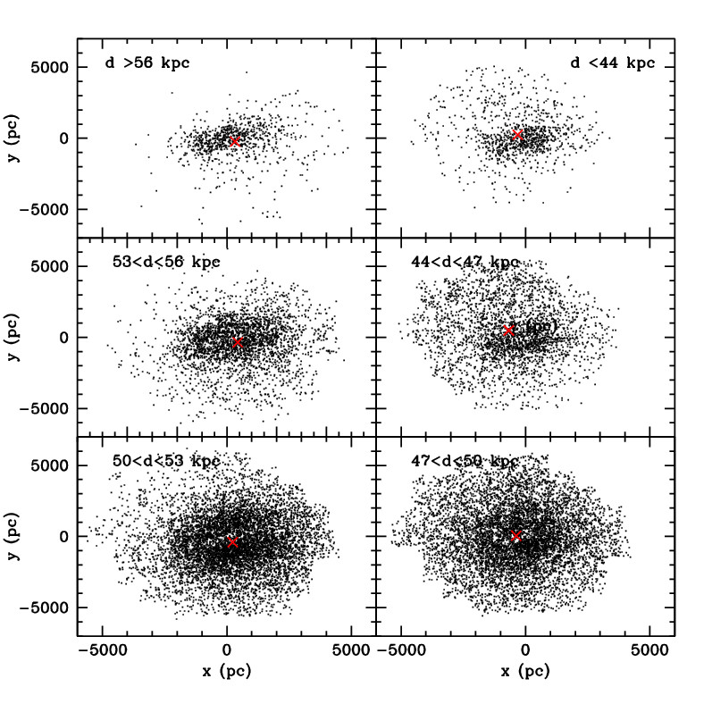
Figure 10: LMC RRLs divided into bins of heliocentric distance, as indicated by the labels. The average centre of the distribution in each panel is marked with a red cross.

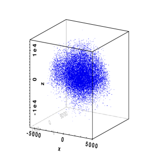
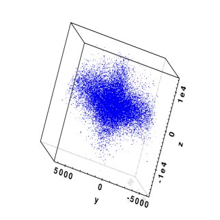
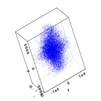
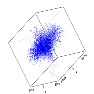
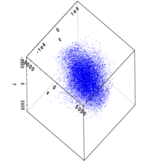
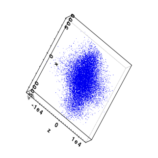
Figure 11: 3-D shape of the LMC inferred from the RRLs, as seen from different viewing angles. The protrusion of sources extending from the LMC centre could be due to crowding effects. Units along the axes are parsecs.

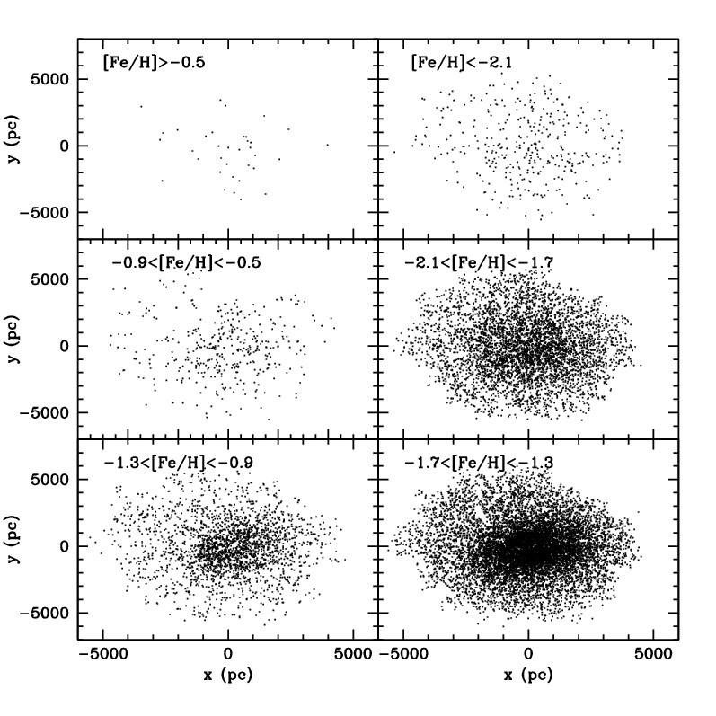
Figure 12: LMC RRLs divided into bins of metallicity, as indicated by the labels.

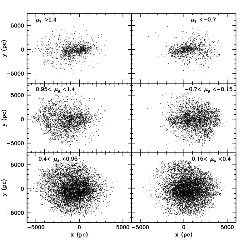
Figure 13: LMC RRLs divided into bins of proper motion in declination, as indicated in the labels.

4.3 Globular Cluster distances

Although neither OGLE IV nor VMC were designed to resolve stars in clusters given their limited spatial resolution, they detected a number of variable stars also in the LMC star clusters. In order to test the 3-D structure of the LMC found in our study, we therefore analysed the RRLs in 3 LMC GCs, namely, NGC 1835, NGC 2210 and NGC 1786, whose RRLs have been observed by OGLE IV (Soszyński et al. 2016). Those stars are mostly found in the periphery of the GCs in less crowded regions. These three GCs were selected because they are located in different regions of the LMC and observed by the VMC survey (see Figure 1). For NGC 1835 (the magenta square in Figure 1), which is located at the western edge of the LMC, there are 9 RRLs (4 RRab and 5 RRc pulsators) in common between the OGLE IV catalogue and our VMC RRL sample. We computed a very tight $PW(K_{\mathrm{s}}$, $J-K_{\mathrm{s}}$) relation from these RRLs, with a scatter of only 0.10 mag. This confirms that the stars are all at the same distance with similar reddening and metallicity, as expected for a GC. The distance to NGC 1835 we found using the RRL $PW(K_{\mathrm{s}}$, $J-K_{\mathrm{s}}$) relation is $d_{\rm NGC1835}$=$52.4\pm 2.3$ kpc. Three of the four RRab stars also have an estimate of the metallicity from Skowron et al. (2016). Their average value is [Fe/H]$\sim-$1.84 dex, in agreement with literature values (see e.g. Walker, 1993; Olsen et al., 1998). We applied the same procedure to NGC 2210 (the blue circle in Figure 1) which is located at the eastern edge of the VMC footprint. The $PW(K_{\mathrm{s}}$, $J-K_{\mathrm{s}}$) relation, based on 8 RRLs in the cluster, is also very tight with a scatter of 0.09 mag which leads to a distance to NGC 2210 of $d_{\rm NGC2210}$= $47.6\pm 2.3$ kpc. Located $\sim$ 1.5 degrees to the north of NGC 1835 the GC NGC 1786 (the green triangle in Figure 1) has 5 RRLs in common between the VMC and OGLE catalogues which leads to a $PW$ relation with a scatter of only 0.08 mag. The average distance to these stars is $d_{\rm NGC1786}$=$49.9\pm 2.4$ kpc. Although the distances of the three clusters are consistent within one sigma there is a hint that, as found in the previous section, the eastern part of the LMC is closer to us than the western part.

5 Discussion and Conclusions

We have obtained new NIR ($K_{\mathrm{s}}$-, $J$- and $Y$-band) and optical ($I$-band) $PL$, $PW$, $PLZ$ and $PWZ$ relations from a sample of $\sim 22,000$ RRLs in the LMC using the VMC, OGLE IV and Gaia data sets. Our starting sample comprised more than $\sim 29,000$ RRLs with a counterpart in the VMC catalogue. However, about $\sim 7,000$ RRLs located in the central, very crowded regions of the LMC were discarded using a 3-$\sigma$ clipping procedure and the matching radius criterion, since they were overluminous with respect to the $PL/PW$ relations. A similar effect was found in the OGLE IV data by Jacyszyn-Dobrzeniecka et al. (2017), who started with an original sample of 27,500 RRab stars and ended up with their final fit being based on a subset of about $\sim 19,500$ of them. Our sample of $\sim 22,000$ RRLs is the largest sample of RRLs used to date to obtain NIR $PL$s. Previous NIR-PL relations available in the literature were based on limited samples (see e.g. Borissova et al., 2009, based on $\sim$40 RRLs) and small fields of view (e.g. Sollima et al., 2006). Moreover, this is the first set of $PLZ$ and $PWZ$ relations in the $Y$-band for RRLs in the LMC. Future facilities like James Webb Space Telescope (JWST) and The Extremely Large Telescope (ELT) will allow the detection of RRLs in galaxies in the Virgo cluster $\sim 20$ Mpc away from us. The rms of the relations we have obtained is good enough that RRLs with just one phase point on their NIR light curves will be sufficient to get an estimate of distance moduli accurate up to $\sim 0.15$ mag. Along with future observations of RRLs in galaxies outside the Local Group, our relations can thus be used to improve the calibration of the cosmic distance ladder.

The comparison of our $PLZ$ relations with the theoretical relations of Marconi et al. (2015) and with observed $PLZ$ in the literature (Muraveva et al., 2018a; Neeley et al., 2019; Braga et al., 2018) indicates that the dependence on metallicity is more significant for high metallicities. However, the LMC lacks such metal-rich RRLs, hence biasing the comparison between theoretical and empirical relations.

Applying the relation of Piersimoni et al. (2002) we derived individual reddening estimates for the RRab stars and obtained a reddening map for the whole LMC. This map was used to provide a reddening estimate for all RRLs in our sample.

R.A. and Dec. coordinates of the LMC centre were derived from the average position of the RRLs and found to be at $\alpha_{0}=80^{\circ}.6147,\delta_{0}=-69^{\circ}.5799$. This agrees within 2^∘ of almost all centre estimates available in the literature (e.g. Nikolaev et al., 2004, based on CCs; van der Marel & Kallivayalil 2014, for other tracers). The same authors also showed that the choice of the centre influences the 3D-shape reconstruction of the LMC, but that differences are rather small and change the determination of the inclination and position angle by only a few degrees.

We used our $PL_{K_{\mathrm{s}}}$ relation to estimate individual distances to $\sim 22,000$ RRLs and from them we reconstructed the 3-D structure of the LMC, as traced by these Population II stars. The LMC resembles a regular ellipsoid with an axes ratio of 1:1.2:1.8, where the north-eastern part of the ellipsoid is closer to us. The position angle and orientation of the bar identified by El Youssoufi et al. (2019) (see Figure 5 in their paper), resembles the band devoid of RRLs seen in our Figure 10 ($50<d<53$ kpc panel). A lack of RRLs in this region is likely caused by the significant crowding conditions in the bar, which prevents the determination of good centroids for the RRLs as well as a proper estimate of their magnitudes. Therefore, we did not directly detect the LMC bar using the RRLs, in agreement with a previous study based on OGLE IV data and optical $PW$ relations (Jacyszyn-Dobrzeniecka et al., 2017).

A protrusion of stars extending on both sides from the centre of the LMC might be the result of blended sources which are still present in our sample notwithstanding the selection steps we performed. These blended sources are very difficult to eliminate since they mix together in every parameter space. However, it is very unlikely that this structure represents a real streaming of RRLs caused by the SMC/LMC interaction. Besla et al. (2012) presented two models of possible past interactions between the SMC and LMC, of which one is a direct collision. These models allow a good reproduction of different peculiar features of both galaxies, but in neither simulations there is a hint of a stellar component projected from the centre of the LMC along the $|z|$ direction.

Using metallicities from Skowron et al. (2016) for a subsample of $\sim$ 13,000 LMC RRab stars and for $\sim$ 5,000 RRc stars using metal abundances derived from our metallicity map we determined $PLZ$ and $PWZ$ relations in the VMC ($Y$, $J$ and $K_{\mathrm{s}}$) and optical ($I$) OGLE IV passbands. We also studied the 3-D spatial distribution of the RRLs based on their metallicities and we did not detect any metallicity gradient or substructure, confirming previous findings (e.g. Deb & Singh, 2014).

Gaia eDR3 proper motions are available for a sample of $\sim 21,000$ RRLs in the VMC catalogue. We used the proper motions to select RRLs which are bona fide members of the LMC and derived a $PL_{K_{\mathrm{s}}}$ which is fully consistent with the relation derived from the full RRL sample. Using the Gaia eDR3 proper motions we also detected the rotation of the LMC as traced by its $>$ 10 Gyr old stars, in full agreement with Gaia Collaboration et al. (2018b) and Gaia Collaboration et al. (2020c) which used a larger sample ($\sim 8$ million) of LMC stars. Some of the RRLs that possess large proper motions, compared with the average value, and are located on the side closer to us, can also be attributed to tidal stream components pointing towards the MW.

Table 4: Parameters of the $PL$ and $PLZ$ relations in different passbands. The coefficients are for the fits in the form: $m_{X0}=a+b\times\log P+c\times$[Fe/H]

Mode	Band	$a$	$\sigma_{a}$	$b$	$\sigma_{b}$	$c$	$\sigma_{c}$	rms	$N_{\rm star}$
FU	$K_{\mathrm{s0}}$	17.360	0.005	$-$2.84	0.02			0.14	16897
FO	$K_{\mathrm{s}0}$	16.860	0.023	$-$2.98	0.05			0.17	5236
Glob	$K_{\mathrm{s}0}$	17.430	0.004	$-$2.53	0.01			0.15	22122
FU	$K_{\mathrm{s}0}$	17.547	0.008	$-$2.80	0.02	0.114	0.004	0.13	13081
FO	$K_{\mathrm{s}0}$	16.850	0.026	$-$2.99	0.05	0.011	0.012	0.17	5132
Glob	$K_{\mathrm{s}0}$	17.603	0.007	$-$2.41	0.01	0.096	0.004	0.15	17698
FU	$J_{0}$	17.699	0.005	$-$2.50	0.02			0.15	16868
FO	$J_{0}$	17.241	0.022	$-$2.53	0.04			0.17	5225
Glob	$J_{0}$	17.800	0.004	$-$2.00	0.01			0.16	22087
FU	$J_{0}$	17.888	0.008	$-$2.45	0.02	0.121	0.004	0.14	13081
FO	$J_{0}$	17.225	0.030	$-$2.53	0.05	-0.010	0.012	0.17	4946
Glob	$J_{0}$	17.962	0.007	$-$1.91	0.01	0.095	0.004	0.15	17757
FU	$Y_{0}$	17.990	0.006	$-$2.25	0.02			0.17	16866
FO	$Y_{0}$	17.550	0.025	$-$2.26	0.05			0.20	5211
Glob	$Y_{0}$	18.110	0.046	$-$1.66	0.02			0.18	22071
FU	$Y_{0}$	18.207	0.009	$-$2.18	0.03	0.135	0.005	0.16	13081
FO	$Y_{0}$	17.553	0.033	$-$2.27	0.05	0.003	0.014	0.19	4946
Glob	$Y_{0}$	18.297	0.008	$-$1.55	0.02	0.108	0.004	0.17	17783
FU	$I_{0}$	18.220	0.005	$-$2.06	0.02			0.13	16696
FO	$I_{0}$	17.830	0.023	$-$1.99	0.05			0.18	5142
Glob	$I_{0}$	18.350	0.004	$-$1.42	0.01			0.15	21838
FU	$I_{0}$	18.439	0.006	$-$1.98	0.02	0.136	0.003	0.11	13081
FO	$I_{0}$	18.439	0.006	$-$1.98	0.02	0.136	0.003	0.11	13081
Glob	$I_{0}$	18.521	0.006	$-$1.36	0.01	0.106	0.003	0.13	17757

Table 5: Parameters of the $PW$ and $PWZ$ relations in different passbands. The parameters are for the fits given in the form: $m_{X}-R\times(m_{Y}-m_{X})=a+b\times\log P+c\times$[Fe/H]

Mode	Band	$R$	$a$	$\sigma_{a}$	$b$	$\sigma_{b}$	$c$	$\sigma_{c}$	rms	$N_{\rm star}$
FU	$K_{\mathrm{s}}$, $J-K_{\mathrm{s}}$	0.69	17.150	0.006	$-$3.075	0.025			0.17	16911
FO	$K_{\mathrm{s}}$, $J-K_{\mathrm{s}}$	0.69	16.600	0.055	$-$3.289	0.027			0.21	5274
Glob	$K_{\mathrm{s}}$, $J-K_{\mathrm{s}}$	0.69	17.190	0.004	$-$2.888	0.016			0.18	22185
FU	$K_{\mathrm{s}}$, J-$K_{\mathrm{s}}$	0.69	17.330	0.009	$-$3.033	0.027	0.111	0.004	0.16	13081
FO	$K_{\mathrm{s}}$, J-$K_{\mathrm{s}}$	0.69	16.619	0.033	$-$3.280	0.052	0.008	0.013	0.19	4945
Glob	$K_{\mathrm{s}}$, J-$K_{\mathrm{s}}$	0.69	17.348	0.008	$-$2.810	0.016	0.094	0.004	0.17	17670
FU	$K_{\mathrm{s}}$, $Y-K_{\mathrm{s}}$	0.42	17.110	0.006	$-$3.086	0.024			0.16	16911
FO	$K_{\mathrm{s}}$, $Y-K_{\mathrm{s}}$	0.42	16.580	0.026	$-$3.276	0.053			0.20	5274
Glob	$K_{\mathrm{s}}$, $Y-K_{\mathrm{s}}$	0.42	17.150	0.004	$-$2.888	0.015			0.17	22185
FU	$K_{\mathrm{s}}$, $Y-K_{\mathrm{s}}$	0.42	17.298	0.009	$-$3.049	0.026	0.107	0.004	0.15	13081
FO	$K_{\mathrm{s}}$, $Y-K_{\mathrm{s}}$	0.42	16.591	0.031	$-$3.270	0.050	0.008	0.013	0.18	4946
Glob	$K_{\mathrm{s}}$, $Y-K_{\mathrm{s}}$	0.42	17.306	0.007	$-$2.813	0.016	0.088	0.004	0.16	17757
FU	$K_{\mathrm{s}}$, I-$K_{\mathrm{s}}$	0.25	17.160	0.006	$-$3.036	0.023			0.16	16686
FO	$K_{\mathrm{s}}$, I-$K_{\mathrm{s}}$	0.25	16.610	0.026	$-$3.243	0.052			0.20	5142
Glob	$K_{\mathrm{s}}$, I-$K_{\mathrm{s}}$	0.25	17.210	0.004	$-$2.800	0.015			0.17	21543
FU	$K_{\mathrm{s}}$, I-$K_{\mathrm{s}}$	0.25	17.337	0.009	$-$2.999	0.027	0.110	0.004	0.15	13081
FO	$K_{\mathrm{s}}$, I-$K_{\mathrm{s}}$	0.25	16.629	0.033	$-$3.217	0.052	0.004	0.013	0.19	4937
Glob	$K_{\mathrm{s}}$, I-$K_{\mathrm{s}}$	0.25	17.368	0.008	$-$2.711	0.016	0.091	0.004	0.16	17567
FU	$K_{\mathrm{s}}$, $V-K_{\mathrm{s}}$	0.13	17.170	0.005	$-$3.021	0.022			0.15	16686
FO	$K_{\mathrm{s}}$, $V-K_{\mathrm{s}}$	0.13	16.630	0.024	$-$3.216	0.048			0.18	5142
Glob	$K_{\mathrm{s}}$, $V-K_{\mathrm{s}}$	0.13	17.220	0.004	$-$2.787	0.014			0.16	21828
FU	$K_{\mathrm{s}}$, $V-K_{\mathrm{s}}$	0.13	17.349	0.008	$-$2.985	0.025	0.109	0.004	0.14	13081
FO	$K_{\mathrm{s}}$, $V-K_{\mathrm{s}}$	0.13	16.650	0.031	$-$3.193	0.049	0.004	0.013	0.18	4957
Glob	$K_{\mathrm{s}}$, $V-K_{\mathrm{s}}$	0.13	17.380	0.007	$-$2.701	0.015	0.090	0.004	0.15	17230
FU	$J$, $I-J$	0.96	17.190	0.008	$-$2.921	0.035			0.23	16686
FO	$J$, $I-J$	0.96	16.660	0.033	$-$3.056	0.066			0.25	5142
Glob	$J$, $I-J$	0.96	17.270	0.006	$-$2.549	0.022			0.24	21828
FU	$J$, $I-J$	0.96	17.358	0.014	$-$2.903	0.041	0.106	0.007	0.23	13081
FO	$J$, $I-J$	0.96	16.658	0.043	$-$3.040	0.068	-0.007	0.017	0.25	13081
Glob	$J$, $I-J$	0.96	17.425	0.011	$-$2.431	0.023	0.085	0.006	0.23	17757
FU	$J$, $V-J$	0.40	17.220	0.006	$-$2.920	0.027			0.18	16686
FO	$J$, $V-J$	0.40	16.700	0.025	$-$3.038	0.051			0.20	5142
Glob	$J$, $V-J$	0.40	17.280	0.005	$-$2.593	0.017			0.18	21828
FU	$J$, $V-J$	0.40	17.377	0.010	$-$2.897	0.031	0.103	0.005	0.17	13081
FO	$J$, $V-J$	0.40	16.697	0.033	$-$3.027	0.052	$-$0.007	0.013	0.20	4946
FU	$J$, $V-J$	0.40	17.433	0.009	$-$2.493	0.017	0.084	0.005	0.18	17546
FU	$I$, $V-I$	1.55	17.160	0.004	$-$3.016	0.018			0.12	16686
FO	$I$, $V-I$	1.55	16.690	0.018	$-$3.101	0.037			0.14	5142
Glob	$I$, $V-I$	1.55	17.190	0.003	$-$2.843	0.011			0.13	21828
FU	$I$, $V-I$	1.55	17.299	0.006	$-$2.994	0.019	0.090	0.003	0.11	13081
FO	$I$, $V-I$	1.55	16.712	0.024	$-$3.105	0.037	0.018	0.010	0.11	4954
Glob	$I$, $V-I$	1.55	17.323	0.006	$-$2.790	0.012	0.076	0.003	0.12	17456

Data availability

The data underlying this article are available in the article and in its online supplementary material or will be shared on reasonable request to the corresponding author.

References

- Alcock et al. (1997) Alcock C., et al. 1997, AJ, 114, 326
- Bell et al. (2020) Bell C. P. M., Cioni M.-R. L., Wright A. H., et al., 2020, MNRAS.tmp, 2691
- Besla et al. (2012) Besla, G., Kallivayalil, N., Hernquist, L. et al. 2012, MNRAS, 421, 2109
- Borissova et al. (2004) Borissova J., Minniti D., Rejkuba M., et al. 2004, A&A, 423, 97
- Borissova et al. (2006) Borissova J., Minniti D., Rejkuba M., Alves D. 2006, A&A, 460, 459
- Borissova et al. (2009) Borissova J., Rejkuba M., Minniti D., Catelan M., Ivanov V. D. 2009, A&A, 502, 505
- Braga et al. (2018) Braga, V. F., Stetson, P. B., Bono, G. et al. 2018, AJ, 155, 137
- Cardelli et al. (1989) Cardelli J. A., Clayton G. C., Mathis J. S. 1989, ApJ, 345, 245
- Carrera et al. (2008) Carrera R., Gallart C., Hardy E. et al. 2008, AJ, 135, 836
- Carretta et al. (2009) Carretta E., Bragaglia A., Gratton R. G., et al. 2009, A&A, 505, 117
- Cioni et al. (2017) Cioni, M.-R., Ripepi, V., Clementini, G. et al. 2017, EPJWC, 15201008
- Cioni et al. (2011) Cioni M.-R. L., Clementini G., Girardi L., et al. 2011, A&A, 527, A116
- Clementini et al. (2000) Clementini G., Di Tomaso S., Di Fabrizio L., et al. 2000, AJ, 120, 2054
- Clementini et al. (2003) Clementini G., Gratton R., Bragaglia A., et al. 2003, AJ, 125, 1309
- Clementini et al. (2019) Clementini G., Ripepi V., Molinaro R., et al. 2019, A&A, 662, A60
- Dalton et al. (2006) Dalton G. B., Caldwell M., Ward A. K., et al. 2006, Proc. SPIE, 6269, id. 62690X
- Deb & Singh (2014) Deb S., Singh H. P. 2014, MNRAS, 438, 2440
- Del Principe et al. (2006) Del Principe M., Piersimoni A. M., Storm J., et al. 2006, ApJ, 652, 362
- Di Criscienzo et al. (2011) Di Criscienzo M., Greco C., Ripepi V., et al. 2011, AJ, 141, 81
- El Youssoufi et al. (2019) El Youssoufi, D., Cioni, M.-R. L.; Bell, C. P. M. et al. 2019, MNRAS, 490, 1076
- Gaia Collaboration, et al. (2016a) Gaia Collaboration, et al., 2016a, A&A, 595, A1
- Gaia Collaboration, et al. (2016b) Gaia Collaboration, et al., 2016b, A&A, 595, A2
- Gaia Collaboration, et al. (2018a) Gaia Collaboration, et al., 2018a, A&A, 616, A1
- Gaia Collaboration et al. (2018b) Gaia Collaboration, et al., 2018b, A&A, 616, A12
- Gaia Collaboration, Brown et al. (2020) Gaia Collaboration, Brown A. G. A. et al. 2020, arXiv:2012.01533
- Gaia Collaboration et al. (2020c) Gaia Collaboration, Luri X., et al. 2020, arXiv:2012.01771
- Gonzalez-Fernandez et al. (2018) González-Fernández, C., Hodgkin, S. T., Irwin, M. J. et al. 2018, MNRAS, 474, 5459
- Gratton et al. (2004) Gratton R. G., Bragaglia A., Clementini G., Carretta E., Di Fabrizio L., Maio M., Taribello E. 2004, A&A, 421, 937
- Iben (1974) Iben I., Jr. 1974, ARA&A 12, 215
- Jacyszyn-Dobrzeniecka et al. (2017) Jacyszyn-Dobrzeniecka A. M., Skowron D. M., Mróz P., et al. 2017, Acta Astron., 67, 1
- Jurcsik & Kovács (1996) Jurcsik J., Kovacs G. 1996, A&A, 312, 111
- Kato et al. (2007) Kato D., Nagashima C., Nagayama T., et al. 2007, PASJ, 59, 615
- Kerber et al. (2009) Kerber L. O., Girardi L., Rubele S., Cioni M.-R. L. 2009, A&A, 499, 697
- Longmore et al. (1986) Longmore A. J., Fernley J. A., Jameson R. F. 1986, MNRAS, 220, 279
- Madore (1982) Madore B. F. 1982, ApJ, 253, 575
- Madore & van den Bergh (1975) Madore B. F., van den Bergh S. 1975, ApJ, 197, 55
- Marconi et al. (2015) Marconi M., Coppola G., Bono G., et al. 2015, ApJ, 808, 50
- Mighell (1999) Mighell K. J. 1999, ApJ, 518, 380
- Morgan et al. (2007) Morgan S. M., Wahl J. N., Wieckhorst R. M. 2007, MNRAS, 374, 1421
- Moretti et al. (2014) Moretti M. I., Clementini G., Muraveva T., et al. 2014, MNRAS, 437, 2702
- Moretti et al. (2016) Moretti M. I., Clementini G., Ripepi V., et al. 2016, MNRAS, 459, 1687
- Muraveva et al. (2014) Muraveva T., Clementini G., Maceroni C., et al. 2014, MNRAS, 443, 432
- Muraveva et al. (2015) Muraveva T., Palmer M., Clementini G., et al. 2015, ApJ, 807, 127
- Muraveva et al. (2018a) Muraveva T., Delgado H. E., Clementini G. et al. 2018a, MNRAS, 481, 1195
- Muraveva et al. (2018b) Muraveva T., Subramanian S., Clementini G., et al. 2018b, MNRAS, 473, 3131
- Neeley et al. (2019) Neeley J. R., Marengo M., Freedman W. L. et al. 2019, MNRAS, 490, 4254
- Nemec et al. (1994) Nemec J. M., Nemec A. F. L., Lutz T. E. 1994, AJ, 108, 222
- Nemec et al. (2013) Nemec J. M., Cohen J. G., Ripepi V., et al. 2013, ApJ, 773, 181
- Nikolaev et al. (2004) Nikolaev, S., Drake, A. J., Keller, S. C. et al. 2004, ApJ, 601, 260
- Olsen et al. (1998) Olsen K. A. G., Hodge P. W., Mateo M., et al. 1998, MNRAS, 300, 665
- Piersimoni et al. (2002) Piersimoni A. M., Bono G., Ripepi V. 2002, AJ, 124, 1528
- Pietrzyński et al. (2013) Pietrzyński G., Graczyk D., Gieren W., et al. 2013, Nature, 495, 76
- Ripepi et al. (2012a) Ripepi V., Moretti M. I., Clementini G., et al. 2012a, Ap&SS, 69
- Ripepi et al. (2012b) Ripepi V., Moretti M. I., Marconi M., et al. 2012b, MNRAS, 424, 1807
- Ripepi et al. (2014) Ripepi V., Marconi M., Moretti M. I., et al. 2014, MNRAS, 437, 2307
- Ripepi et al. (2015) Ripepi V., Moretti M. I., Marconi M., et al. 2015, MNRAS, 446, 3034
- Ripepi et al. (2016) Ripepi V., Marconi M., Moretti M. I., et al. 2016, ApJS, 224, 21
- Ripepi et al. (2017) Ripepi V., Cioni M.-R. L., Moretti M. I., et al. 2017, MNRAS, 472, 808
- Rubele et al. (2012) Rubele S., Kerber L., Girardi L., et al. 2012, A&A, 537, A106
- Rubele et al. (2015) Rubele S., Girardi L., Kerber L., et al. 2015, MNRAS, 449, 639
- Rubele et al. (2018) Rubele S., Pastorelli G., Girardi L., et al. 2018, MNRAS, 478, 5017
- Sandage (1981a) Sandage A. 1981, ApJL, 244, L23
- Sandage (1981b) Sandage A. 1981, ApJ, 248, 161
- Sesar et al. (2017b) Sesar B., Fouesneau M., Price-Whelan A. M., Bailer-Jones C. A. L., Gould A., Rix H.-W., 2017b, ApJ, 838, 107
- Skillen et al. (1993) Skillen I., Fernley J. A., Stobie R. S., Jameson R. F. 1993, MNRAS, 265, 301
- Skowron et al. (2016) Skowron D. M., Soszyński I., Udalski A., et al. 2016, Acta Astron., 66, 269
- Skrutskie et al. (2006) Skrutskie M. F., Cutri R. M., Stiening R., et al. 2006, AJ, 131, 1163
- Sollima et al. (2006) Sollima A., Cacciari C., Valenti, E., 2006, MNRAS, 372, 1675
- Sollima et al. (2008) Sollima A., Cacciari C., Arkharov A. A. H., et al. 2008, MNRAS, 384, 1583
- Soszyński et al. (2009) Soszyński I., Udalski A., Szymański M. K., et al. 2009, Acta Astron., 59, 1
- Soszyński et al. (2012) Soszyński I., Udalski A., Poleski R., et al. 2012, Acta Astron., 62, 219
- Soszyński et al. (2016) Soszyński I., Udalski A., Szymański M. K., et al. 2016, Acta Astron., 66, 131
- Soszyński et al. (2019) Soszyński I., Udalski A., Szymański M. K., et al. 2019, Acta Astron., 69, 87
- Subramanian et al. (2017) Subramanian, S., Rubele, S., Sun, N.-C. et al. 2017, MNRAS, 467, 2980
- Szewczyk et al. (2008) Szewczyk O., et al. 2008, AJ , 136, 272
- Tatton et al. (2013) Tatton B. L., van Loon, J. T. Cioni, M.-R. L., et al. 2013, A&A, 554, A33
- Tisserand et al. (2007) Tisserand P., et al. 2007, A&A, 469, 387
- Udalski et al. (1997) Udalski, A. Kubiak M., Szymanski M. 1997, Acta Astron., 47, 319
- van Albada & Baker (1971) van Albada T. S., Baker N. 1971, ApJ, 169, 311
- van den Bergh (1975) van den Bergh, S. 1993, MNRAS, 262, 588
- van der Marel & Cioni (2001) van der Marel R. P., Cioni M.-R. L. 2001, AJ, 122, 1807
- van der Marel & Cioni (2001) van der Marel R. P., Kallivayalil N. 2014, ApJ, 781, 121
- Walker (1993) Walker A. R. 1993, AJ, 105, 527
- Weinberg & Nikolaev (2001) Weinberg M. D., Nikolaev S., 2001, ApJ, 548, 712
- Zinn & West (1984) Zinn R., West M. J., 1984, ApJS, 55, 45