Abstract

We present a novel method for single image depth estimation using surface normal constraints. Existing depth estimation methods either suffer from the lack of geometric constraints, or are limited to the difficulty of reliably capturing geometric context, which leads to a bottleneck of depth estimation quality. We therefore introduce a simple yet effective method, named Adaptive Surface Normal (ASN) constraint, to effectively correlate the depth estimation with geometric consistency. Our key idea is to adaptively determine the reliable local geometry from a set of randomly sampled candidates to derive surface normal constraint, for which we measure the consistency of the geometric contextual features. As a result, our method can faithfully reconstruct the 3D geometry and is robust to local shape variations, such as boundaries, sharp corners and noises. We conduct extensive evaluations and comparisons using public datasets. The experimental results demonstrate our method outperforms the state-of-the-art methods and has superior efficiency and robustness .

1 Introduction

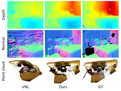
Figure 1: Example results of ground truth, ours and VNL [46]. By enforcing our proposed Adaptive Surface Normal (ASN) constraint, our reconstructed point cloud preserves both global structural information and local geometric features. The recovered surface normal is more accurate and less noisy than that of VNL.

Estimating depth from a single RGB image, one of the most fundamental computer vision tasks, has been extensively researched for decades. With the recent advances of deep learning, depth estimation using neural networks has drawn increasing attention. Earlier works [6, 22, 9, 34, 31] in this field directly minimize the pixel-wise depth errors, of which results cannot faithfully capture the 3D geometric features. Therefore, the latest efforts incorporate geometric constraints into the network and show promising results.

Among various geometric attributes, surface normal is predominantly adopted due to the following two reasons. First, surface normal can be estimated by the 3D points converted from depth. Second, surface normal is determined by a surface tangent plane, which inherently encodes the local geometric context. Consequently, to extract normals from depth maps as geometric constraints, previous works propose various strategies, including random sampling [46], Sobel-like operator [13, 16] and differentiable least square [28, 26].

Despite the improvements brought about by the existing efforts, a critical issue remains unsolved, i.e., how to determine the reliable local geometry to correlate the normal constraint with the depth estimation. For example, at shape boundaries or corners, the neighboring pixels for a point could belong to different geometries, where the local plane assumption is not satisfied. Due to this challenge, these methods either struggle to capture the local features [46], or sensitive to local geometric variations (noises or boundaries) [13, 16], or computationally expensive [28, 26].

Given the significance of local context constraints, there is a multitude of works on how to incorporate shape-ware regularization in monocular reconstruction tasks, ranging from sophisticated variational approaches for optical flow [33, 41, 32, 1] to edge-aware filtering in stereo [36] and monocular reconstruction [14, 29]. However, these methods have complex formulations and only focus on 2D feature edges derived from image intensity variation, without considering geometric structures of shapes in 3D space.

In this paper, we introduce a simple yet effective method to correlate depth estimation with surface normal constraint. Our formulation is much simpler than any of the aforementioned approaches, but significantly improves the depth prediction quality, as shown in Fig. 1. Our key idea is to adaptively determine the faithful local geometry from a set of randomly sampled candidates to support the normal estimation. For a target point on the image, first, we randomly sample a set of point triplets in its neighborhood to define the candidates of normals. Then, we determine the confidence score of each normal candidate by measuring the consistency of the learned latent geometric features between the candidate and the target point. Finally, the normal is adaptively estimated as a weighted sum of all the candidates.

Our simple strategy has some unique advantages: 1) the random sampling captures sufficient information from the neighborhood of the target point, which is not only highly efficient for computation, but also accommodates various geometric context; 2) the confidence scores adapatively determine the reliable candidates, making the normal estimation robust to local variations, e.g., noises, boundaries and sharp changes; 3) we measure the confidence using the learned contextual features, of which representational capacity is applicable to complex structures and informative to correlate the normal constraint with the estimated depth. More importantly, our method achieves superior results on the public datasets and considerably outperforms the state-of-the-art methods.

Our main contributions are summarized as follows:

• We introduce a novel formulation to derive geometric constraint for depth estimation, i.e., adaptive surface normal.

• Our method is simple, fast and effective. It is robust to noises and local variations and able to consistently capture faithful geometry.

• Our method outperforms the state-of-the-art method on the public datasets by a large margin.

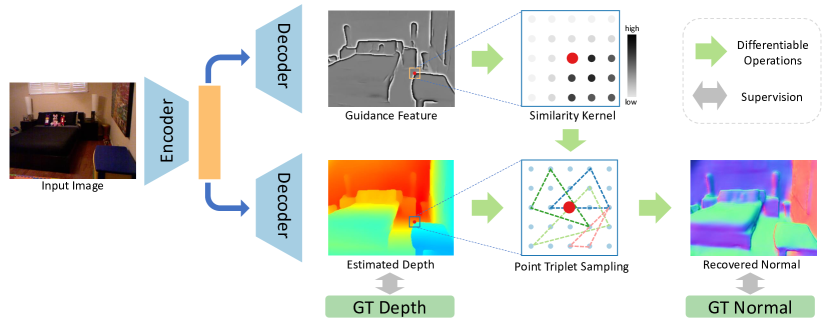
Figure 2: Overview of our method. Taking a single image as input, our model produces estimated depth and guidance feature from two decoders, respectively. We recover surface normal from the estimated depth map with our proposed Adaptive Surface Normal (ASN) computation method. The similarity kernels computed from guidance feature enable our surface normal calculation to be local geometry aware, like shape boundaries and corners. Finally, pixel-wise depth supervision is enforced on the estimated depth, while the geometric supervision is enforced on the recovered surface normal.

2 Related Work

Monocular depth estimation

As an ill-posed problem, monocular depth estimation is challenging, given that minimal geometric information can be extracted from a single image. Recently, benefiting from the prior structural information learned by the neural network, many learning-based works [6, 22, 43, 9, 34, 31, 11, 10, 24, 23] have achieved promising results. Eigen et al. [6] directly estimate depth maps by feeding images into a multi-scale neural network. Laina et al. [18] propose a deeper residual network and further improve the accuracy of depth estimation. Liu et al. [22] utilize a continuous conditional random field (CRF) to smooth super-pixel depth estimation. Xu et al. [43] propose a sequential network based on multi-scale CRFs to estimate depth. Fu et al. [9] design a novel ordinal loss function to recover the ordinal information from a single image. Unfortunately, the estimated depth maps of these methods always fail to recover important 3D geometric features when converted to point clouds, since these methods do not consider any geometric constraints.

Joint depth and normal estimation

Since the depth and surface normal are closely related in terms of 3D geometry, there has been growing interests in joint depth and normal estimation using neural networks to improve the performance. Several works [5, 47, 42, 20] jointly estimate depth and surface normal using multiple branches and propagate the latent features of each other. Nevertheless, since there are no explicit geometric constraints enforced on the depth estimation, the predicted geometry of these methods is still barely satisfactory.

Consequently, methods [44, 45, 30, 13, 28, 26, 16] are proposed to explicitly enforce geometric constraints on estimated depth maps.. Hu et al. [13] and Kusupati etal [16] utilize a Sobel-like operator to calculate surface normals from estimated depths, and then enforce them to be consistent with the ground truth. Nonetheless, the Sobel-like operator can be considered as a fixed filter kernel that indiscriminately acts on the whole image (see Fig. 3), leading to unacceptable inaccuracy and sensitivity to noises. To constrain surface normal more reliably, Qi et al. [28] and Long et al. [26] propose to utilize a differentiable least square module for surface normal estimation. These methods optimize the geometric consistency, of which solution is more accurate and robust to noises but limited to expensive computation. Yin et al. [46] introduce virtual normal, which is a global geometric constraint derived from the randomly sampled point triplets from estimated depth. However, this constraint struggles to capture local geometric features, given that the point triplets are randomly sampled from the whole image.

Edge preserving methods

Out of the statistical relations between shape boundaries and image intensity edges, many works leverage this statistic prior to benefit many vision tasks. Anisotropic diffusion [27, 2, 40] is a well-known technique for image denoising without removing important details of image content, typically edges. Works [33, 41, 32, 1] propose variational approaches with anisotropic diffusion to model local edge structures for optical flow estimation. Some stereo/monocular depth estimation works rely on pretrained edge detection network [36] or Canny edge detector [14, 29], to extract image edges to improve depth estimation. However, only a small fraction of the intensity edges keep consistent with true geometric shape boundaries. Our method could detect the true shape boundaries where 3D geometry changes instead of image intensity edges.

3 Method

Given a single color image $I$ as input, we use an encoder-decoder neural network to output its depth map $D_{pred}$. Our approach aims to not only estimate accurate depth but also recover high-quality 3D geometry. For this purpose, we correlate surface normal constraint with depth estimating. Overall, we enforce two types of supervision for training the network. First, like most of depth estimation works, we employ a pixel-wise depth supervision like $L_{1}$ loss over the predicted depth $D_{pred}$ and ground truth depth $D_{gt}$. Moreover, we compute the surface normal $N_{pred}$ from $D_{pred}$ using an adaptive strategy, and enforce consistency between $N_{pred}$ with the ground truth surface normal $N_{gt}$, named as Adaptive Surface Normal (ASN) constraint. The method is overviewed in Fig. 2.

Local plane assumption.

To correlate surface normal constraint with depth estimation, we adopt the local plane assumption following  [28, 26]. That is, a small set of neighborhoods of a point forms a local plane, of which normal vector approximates the surface normal. Hence, for a pixel on the depth map, its surface normal can be estimated by the local patch formed by its neighboring points. In theory, the local patch could have arbitrary shapes and sizes. In practice, however, square local patches are widely adopted with sizes $(2m+1)\times(2m+1),m=1,2,...,n$, due to its simplicity and efficiency.

Normal candidates sampling.

To compute the surface normal, unlike prior works utilize least square fitting  [28, 26] or Sobel-like kernel approximation  [13, 16], we propose a randomly sampling based strategy.

For a target point $P_{i}\in\mathbb{R}^{3}$, we first extract all the points $\mathbb{P}_{i}=\left\{P_{j}\mid P_{j}\in\mathbb{R}^{3},\ j=0,\ldots,r^{2}-1\right\}$ within a local patch of size $r\times r$. Then, we randomly sample $K$ point triplets in $\mathbb{P}_{i}$. All sampled point triplets for the target point $P_{i}$ are denoted as $\mathbb{T}_{i}=\left\{\left(P_{k}^{A},P_{k}^{B},P_{k}^{C}\right)\mid P\in\mathbb{R}^{3},\ k=0,\ldots,K-1\right\}$. If the three points are not colinear, the normal vector of the sampled local plane can be directly computed by the cross-product:

$$\vec{n}_{k}=\frac{\overrightarrow{P_{k}^{A}P_{k}^{B}}\times\overrightarrow{P_{k}^{A}P_{k}^{C}}}{\mid\overrightarrow{P_{k}^{A}P_{k}^{B}}\times\overrightarrow{P_{k}^{A}P_{k}^{C}}\mid}.$$ (1)

A normal vector will be flipped according to the viewing direction if it does not match the camera orientation. In this way, for each target point, we obtain $K$ normal candidates corresponding to $K$ sampled local planes. Next, we adaptively determine the confidence of each candidate to derive the final normal estimation result.

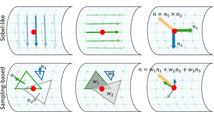
Figure 3: Sobel-like operator versus ours for surface normal estimation. The Sobel-like operator first calculates two principle vectors along up-down and left-right directions, and then use their cross product to estimate the normal. Ours first computes the normal vectors of the randomly sampled triplets, and then adaptively combines them together to obtain the final estimation.

Geometric context adaption.

We observe that the neighbors of a target point may not lie in the same tangent plane, especially at a region where the geometry changes, e.g., shape boundaries or sharp corners. Thus, we propose to learn a guidance feature map that is context aware to reflect the geometric variation. Therefore, the network can determine the confidence of the neighboring geometry by measuring the learned context features.

Given the learned guidance feature map, we measure the $L_{2}$ distance of the features of a sampled point $P_{j}$ and the target point $P_{i}$, and then use a normalized Gaussian kernel function to encode their latent distance into $[0,1]$:

$$\mathcal{L}\left(P_{i},P_{j}\right) =e^{-0.5\left\|f\left(P_{i}\right)-f\left(P_{j}\right)\right\|_{2}}$$ (2)

$$\overline{\mathcal{L}}\left(P_{i},P_{j}\right) =\frac{\mathcal{L}\left(P_{i},P_{j}\right)}{\sum_{P_{n}\in\mathbb{P}_{i}}\mathcal{L}\left(P_{i},P_{n}\right)},$$

where $f(\cdot)$ is the guidance feature map, $\left\|\cdot\right\|_{2}$ is $L_{2}$ distance, and $\mathbb{P}_{i}$ is the neighboring point set in the local patch of $P_{i}$ as aforementioned. E.q. 2 gives a confidence score, where the higher the confidence is, the more likely the two is to locate in the same tangent plane with target pixel. Accordingly, the confidence score of a local plane $(P_{k}^{A},P_{k}^{B},P_{k}^{C})$ to the center point $P_{i}$ given by the geometric adaption is defined by:

$$g_{k}=\prod_{t=A,B,C}\overline{\mathcal{L}}\left(P_{i},P_{k}^{t}\right).$$ (3)

This is the multiplication of three independent probabilistic scores of the three sampled points, which measures the reliability of a sampled local plane.

Area adaption.

The area of a sampled local plane (triangle) is an important reference to determine the reliability of the candidate. A larger triangle captures more information and thus would be more robust to local noise, as shown in  [46]. For a triangle $T_{k}$, we simply consider its projected area $s_{k}$ on the image as a measurement of confidence score. Note that the area is calculated on the 2D image, since the sampled triangles in the 3D space could be very large due to depth variation, leading to unreasonable overestimation.

Finally, the normal for a point $P_{i}$ is determined by a weighted combination of all the $K$ sampled candidates, where the weights represent the confidence given by our adaptive strategy:

$$\vec{n}_{i}=\frac{\sum_{k=0}^{K-1}s_{k}\cdot g_{k}\cdot\vec{n}_{k}}{\sum_{k=0}^{K-1}s_{k}\cdot g_{k}},$$ (4)

where $K$ is the number of sampled triplets, $s_{k}$ is the projected area of three sampled point $(P_{k}^{A},P_{k}^{B},P_{k}^{C})$ on the 2D image, and $n_{k}$ is its normal vector.

4 Implementation

Network architecture

Our network adopts a multi-scale structure, which consists of one encoder and two decoders. We use HRNet-48 [37] as our backbone. Taking one image as input, one encoder produces coarse-to-fine estimated depths in four scales, and the other decoder is used to generate the guidance feature map that captures geometric context. The depth estimation decoder consists of four blocks in different scales, each of which is constituted by two ResNet [12] basic blocks with a feature reducing convolution layer. The appending convolution layers are used to produce one-channel output for depth estimation. The guidance feature encoder adopts a nearly identical structure with the depth encoder but without any feature reducing layers.

Loss functions

Our training loss has two types of terms: depth loss term and surface normal loss term. For the depth term, we use the $L_{1}$ loss for our multi-scale estimation:

$$l_{d}=\sum_{s=0}^{3}\lambda^{s-3}\left\|D_{pred}^{s}-D_{gt}\right\|_{1},$$ (5)

where $D_{pred}^{s}$ means the estimated depth map at $s^{th}$ scale, $D_{gt}$ is the ground truth depth map, and $\lambda$ is a factor for balancing different scales. Here we set $\lambda=0.8$.

To enforce geometric constraint on the estimated depth map, using our proposed adaptive strategy, we compute the surface normals only based on the finest estimated depth map. To regularize the consistency of the computed surface normals with ground truth, we adopt a cosine embedding loss:

$$l_{n}=1-cos(N_{pred},N_{gt}),$$ (6)

where $N_{pred}$ is the surface normal map calculated from the finest estimated depth map, and $N_{gt}$ is the ground truth surface normal. Therefore, the overall loss is defined as:

$$l=l_{d}+\alpha l_{n},$$ (7)

where $\alpha$ is set to 5 in all experiments, which is a trade-off parameter to make the two types of terms roughly of the same scale.

Training details

Our model is implemented by Pytorch with Adam optimizer ($init\_lr=0.0001$, $\beta_{1}=0.9$, $\beta_{2}=0.999$, $weight\_decay=0.00001$). The learning rate is polynomially decayed with polynomial power 0.9. The model is trained with only depth loss term in the first 20 epochs, and then with depth and surface normal loss terms in the last 20 epochs. The whole training is completed with 8 batches on four GeForce RTX 2080 Ti GPUs. We adopt $5\times 5$ local patch and 40 sampling triplets in all experiments.

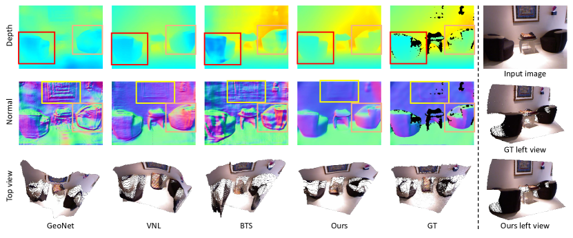
Figure 4: Qualitative comparisons with SOTAs on NYUD-V2. Compared with other methods, our estimated depth is more accurate and contain less noises. The recovered surface normal maps and point clouds demonstrate that our estimated depth faithfully preserve important geometric features. The black regions are the invalid regions lacking ground truth.

5 Experiments

5.1 Dataset

NYUD-V2

Our model is trained on NYUD-V2 dataset. NYUD-V2 is a widely used indoor dataset and contains 464 scenes, of which 249 scenes are for training and 215 for testing. We directly adopt the collected training data provided by Qi et al. [28], which has 30,816 frames sampled from the raw training scenes with precomputed ground truth surface normals. The precomputed surface normals are generated following the procedure of  [7]. Note that DORN [9], Eigen et al. [5], Xu et al. [43], Laina et al. [18], and Hu et al. [13] use 407k, 120k, 90k, 95k and 51k images for training, which are all significantly larger than ours. For testing, we utilize the official test set that is the same as the competitive methods, which contains 654 images.

ScanNet

We also evaluate our method on a recently proposed indoor dataset, ScanNet [4], which has more than 1600 scenes. Its official test split contains 100 scenes, and we uniformly select 2167 images from them for cross-dataset evaluation.

Table 1: Depth evaluation on NYUD-V2 dataset.

Method	rel ($\downarrow$)	log10 ($\downarrow$)	rms ($\downarrow$)	$\boldsymbol{\delta_{1}}$ ($\uparrow$)	$\boldsymbol{\delta_{2}}$ ($\uparrow$)	$\boldsymbol{\delta_{3}}$ ($\uparrow$)
Saxena et al. [35]	0.349	-	1.214	0.447	0.745	0.897
Karsch et al. [15]	0.349	0.131	1.21	-	-	-
Liu et al. [25]	0.335	0.127	1.06	-	-	-
Ladicky et al. [17]	-	-	-	0.542	0.829	0.941
Li et al. [20]	0.232	0.094	0.821	0.621	0.886	0.968
Roy et al. [34]	0.187	0.078	0.744	-	-	-
Liu et al. [22]	0.213	0.087	0.759	0.650	0.906	0.974
Wang et al. [38]	0.220	0.094	0.745	0.605	0.890	0.970
Eigen et al. [5]	0.158	-	0.641	0.769	0.950	0.988
Chakrabarti et al. [3]	0.149	-	0.620	0.806	0.958	0.987
Li et al. [21]	0.143	0.063	0.635	0.788	0.958	0.991
Laina et al. [18]	0.127	0.055	0.573	0.811	0.953	0.988
Hu et al. [13]	0.115	0.050	0.530	0.866	0.975	0.993
DORN [9]	0.115	0.051	0.509	0.828	0.965	0.992
GeoNet [28]	0.128	0.057	0.569	0.834	0.960	0.990
VNL [46]	0.108	0.048	0.416	0.875	0.976	0.994
BTS [19]	0.113	0.049	0.407	0.871	0.977	0.995
Ours	0.101	0.044	0.377	0.890	0.982	0.996

5.2 Evaluation metrics

To evaluate our method, we compare our method with state-of-the-arts in three aspects: accuracy of depth estimation, accuracy of recovered surface normal, and quality of recovered point cloud.

Depth

Following the previous method [6], we adopt the following metrics: mean absolute relative error (rel), mean log10 error (log10), root mean squared error (rms), and the accuracy under threshold ($\delta<{1.25}^{i}\text{ where }i\in\{1,2,3\}$).

Surface normal

Like prior works [5, 28], we evaluate surface normal with the following metrics: the mean of angle error (mean), the median of the angle error (median), and the accuracy below threshold $t\text{ where }t\in\left[11.25^{\circ},22.5^{\circ},30^{\circ}\right]$.

Point cloud

For quantitatively evaluate the point clouds converted from estimated depth maps, we utilize the following metrics: mean Euclidean distance (dist), root mean squared Euclidean distance (rms), and the accuracy below threshold $t\text{ where }t\in\left[0.1m,0.3m,0.5m\right]$.

5.3 Evaluations

Depth estimation accuracy

We compare our method with other state-of-the-art methods on NYUD-V2 dataset. As shown in Table 1, our method significantly outperforms the other SOTA methods across all evaluation metrics. Moreover, to further evaluate the generalization of our method, we compare our method with some strong SOTAs on unseen ScanNet dataset. As shown in Table 2, our method still shows better performance than others.

Besides the quantitative comparison, we show some qualitative results for several SOTA methods that also use geometric constraints, including i) GeoNet [28] (least square normal); ii)VNL [46] (virtual normal constraint); iii) BTS [19] (predict local plane equations not directly predict depth). As shown in Fig. 4, the proposed method faithfully recovers the original geometry. For the regions with high curvatures, such as the sofas, our results obtain cleaner and smoother surfaces; our predicted depth map also yields high-quality shape boundaries, which leads to better accuracy compared to the ground truth depth map. Also, note even for the texture-less walls and floors, our estimated depth is still satisfactory.

Table 2: Depth evaluation on ScanNet dataset.

Method	rel ($\downarrow$)	log10 ($\downarrow$)	rms ($\downarrow$)	$\boldsymbol{\delta_{1}}$ ($\uparrow$)	$\boldsymbol{\delta_{2}}$ ($\uparrow$)	$\boldsymbol{\delta_{3}}$ ($\uparrow$)
GeoNet [28]	0.255	0.106	0.519	0.561	0.855	0.958
VNL [46]	0.238	0.105	0.505	0.565	0.856	0.957
BTS [19]	0.246	0.104	0.506	0.583	0.858	0.951
Ours	0.233	0.100	0.484	0.609	0.861	0.955

Table 3: Point cloud evaluation on NYUD-V2 dataset.

Method	dist ($\downarrow$)	rms ($\downarrow$)	$\boldsymbol{0.1m}$ ($\uparrow$)	$\boldsymbol{0.3m}$ ($\uparrow$)	$\boldsymbol{0.5m}$ ($\uparrow$)
VNL [46]	0.515	0.686	0.181	0.469	0.644
GeoNet [28]	0.392	0.608	0.220	0.558	0.747
BTS [19]	0.317	0.544	0.278	0.653	0.822
Hu et al. [13]	0.311	0.537	0.288	0.666	0.831
Ours	0.266	0.497	0.332	0.727	0.869

Point cloud

From the Table 3, in terms of the quality of point cloud, our method outperforms other methods by a large margin. Surprisingly, although VNL [46] has better performance than GeoNet [28] in terms of depth evaluation errors, its mean Eucleadian distance is worse than GeoNet, which demonstrates the necessity of evaluation specially designed for point clouds. As shown in Fig. 4 (the third row), our point cloud has fewer distortions and much more accurate than others. The point clouds generated from the depth maps of other methods suffer from severe distortions and struggle to preserve prominent geometric features, such as planes (e.g., walls) and surfaces with high curvatures (e.g., sofas). Besides, we also show a qualitative comparison between our point cloud and the ground truth from a different view in Fig. 4. The highly consistent result further demonstrates our method’s superior performance in terms of the quality of 3D geometry.

Surface Normal

As shown in Table 4, our recovered surface normals have considerably better quality than that of the other methods. For reference, we also report the results generated by the methods that directly output normal maps in the network. Surprisingly, the accuracy of our recovered surface normals is even higher than this kind of methods that can explicitly predict normals. Also, we present qualitative comparisons in Fig. 4. It can be seen that our surface normal is smoother and more accurate than the others, which indicates that our strategy is effective for correlating normal constraints with depth estimation, resulting in not only accurate depth estimation, but also reliable surface normals and 3D geometry.

Table 4: Surface normal evaluation on NYUD-V2 dataset.

Method	Mean ($\downarrow$)	Median ($\downarrow$)	$\boldsymbol{11.25^{\circ}}$ ($\uparrow$)	$\boldsymbol{22.5^{\circ}}$ ($\uparrow$)	$\boldsymbol{30^{\circ}}$ ($\uparrow$)
Predicted Surface Normal from the Network
3DP [7]	33.0	28.3	18.8	40.7	52.4
Ladicky et al. [17]	35.5	25.5	24.0	45.6	55.9
Fouhey et al. [8]	35.2	17.9	40.5	54.1	58.9
Wang et al. [39]	28.8	17.9	35.2	57.1	65.5
Eigen et al. [5]	23.7	15.5	39.2	62.0	71.1
Calculated Surface Normal from the Point cloud
BTS [19]	44.0	35.4	14.4	32.5	43.2
GeoNet [28]	36.8	32.1	15.0	34.5	46.7
DORN [9]	36.6	31.1	15.7	36.5	49.4
Hu et al. [13]	32.1	23.5	24.7	48.4	59.9
VNL [46]	24.6	17.9	34.1	60.7	71.7
Ours	20.0	13.4	43.5	69.1	78.6

5.4 Discussions

In this section, we further conduct a series of evaluations with an HRNet-18 [37] backbone to give more insights into the proposed method.

Effectiveness of ASN

To validate the effectiveness of our proposed adaptive surface normal constraint, we train models with different constraints: a) only $L_{1}$ depth constraint; b) depth and Sobel-like operator surface normal constraints (SOSN); c) depth and least square surface normal constraints (LSSN); d) depth and virtual normal constraints (VN); e) depth and our adaptive surface normal constraints (ASN).

As shown in Table 5, the model with our adaptive surface normal constraint outperforms (ASN) all the others. Although the models with Sobel-like operator (SOSN) and least square normal constraint (LSSN) shows better recovered surface normal, their depth estimation accuracy drops off compared with the model without geometric constraint. The model with virtual normal (VN) [46] constraint shows the worst quality of recovered surface normal among the four types of geometric constraints, given that virtual normal is derived from global sampling on the estimated depth map, which inevitably loses local geometric information.

Furthermore, we give a set of qualitative comparisons in Fig. 5. The results clearly show our ASN constraint achieves better surface normal estimation results and captures detailed geometric features, even for the thin structures like the legs of chairs.

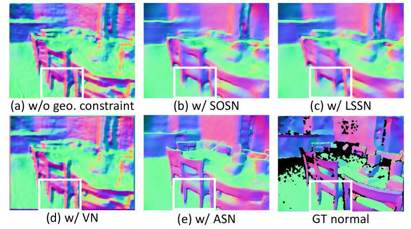
Figure 5: Comparisons of models with different geometric constraints. Model with our ASN constraint achieves better surface normal estimation, even accurately capture detailed geometries, like the legs of chairs (see white boxes).

Table 5: Comparisons of models with different geometric constraints on NYUD-V2 dataset.

Constraints	rel ($\downarrow$)	log10 ($\downarrow$)	$\boldsymbol{\delta_{1}}$ ($\uparrow$)	Mean ($\downarrow$)	Median ($\downarrow$)	$\boldsymbol{11.25^{\circ}}$ ($\uparrow$)
	Depth			Recovered normal
L1	0.113	0.047	0.875	31.3	23.2	24.9
L1 + SOSN	0.118	0.049	0.867	22.8	16.1	36.2
L1 + LSSN	0.119	0.050	0.862	23.5	16.3	35.7
L1 + VN	0.111	0.047	0.876	31.7	21.4	28.4
L1 + ASN	0.111	0.047	0.876	22.2	15.8	36.9

Ablation study of adaptive modules

To evaluate the effect of the proposed two adaptive modules, i.e., geometric context adaption and area adaption, we conduct an ablation study. We train models with different adaptive modules: only Geometric Context (GC) adaption, only Area adaption, and both. From Table 6, we can see the model with both adaptive modules achieves the best performance, which verifies the necessity of each adaptive module.

Table 6: Ablation study of the proposed adaptive modules on NYUD-V2 dataset. We evaluate the accuracy of the recovered surface normals.

Module	Mean ($\downarrow$)	Median ($\downarrow$)	$\boldsymbol{11.25^{\circ}}$ ($\uparrow$)	$\boldsymbol{22.5^{\circ}}$ ($\uparrow$)	$\boldsymbol{30^{\circ}}$ ($\uparrow$)
only Area	22.6	16.0	36.4	63.6	74.4
only GC	22.3	15.8	36.9	64.1	74.8
Area+GC	22.2	15.8	36.9	64.2	74.9

Visualization of guidance features

The geometric adaptive module is the key to our adaptive surface normal constraint method. To better understand what the network learns, we visualize the learned features of the guidance map. We plot one from the multiple channels of the guidance feature map, which is shown in Fig. 6. It can be seen that the learned guidance map captures the shape context and geometric variations, giving informative boundaries.

For comparison, we use the Canny operator to detect the edges of the input image by image intensity variance. As we can see, our guidance feature map is not simply coincident with the Canny edges. For example, in Fig. 6, the Canny operator detects fragmented edges based on the texture of wall painting and sofas, while our guidance feature map indicates the true shape boundaries where the 3D geometry changes.

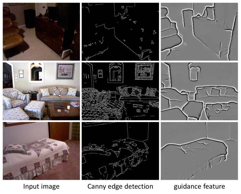
Figure 6: Our guidance feature maps versus edge maps detected by Canny operator. Although shape boundaries have high statistic correlations with image edges, they are not always coincident. Our feature map captures the true geometric boundaries, while the Canny operator detects edges with significant intensity variances.

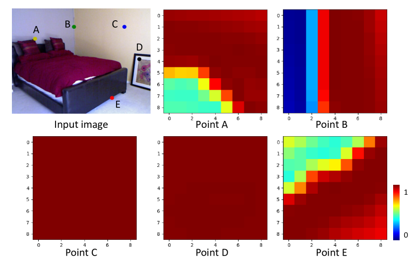
Figure 7: The visualization of similarity kernels. The similarity kernels of Point A, B, and E demonstrate that our method could successfully distinguish different geometries. The similarity kernels of Point C and D further show that our method captures the 3D geometry variances of the shapes in the 3D world, instead of the image color distinctions.

Visualization of similarity kernels

To validate whether our model can capture the true geometric boundaries of shapes, we select five points on the image and visualize their color coded similarity kernels in Fig. 7. The similarity kernels of Point A, B, and E indicate that our method could successfully distinguish different geometries, such as shape boundaries and corners. Furthermore, the similarity kernels of Point C and D show that our approach captures the 3D geometry variances of the shapes in the real world, instead of the color distinctions of the image. For example, Point D has large color variances in the image, but its similarity kernel has constant values indicating the unchanged geometry.

Number of sampled triplets.

To quantitatively analyze the influence of the number of sampled triplets, we recover surface normals from our estimated depth maps using our adaptive surface normal computation method with $5\times 5$ local patch. Based on Fig. 8, it is not surprised that more sampled triplets will contribute to more accurate surface normals. The accuracy increases dramatically from $10\sim 20$ sampled triplets and gradually saturates with more triplets sampled. To balance efficiency and accuracy, the number of sampled triplets is recommended to be $40\sim 60$.

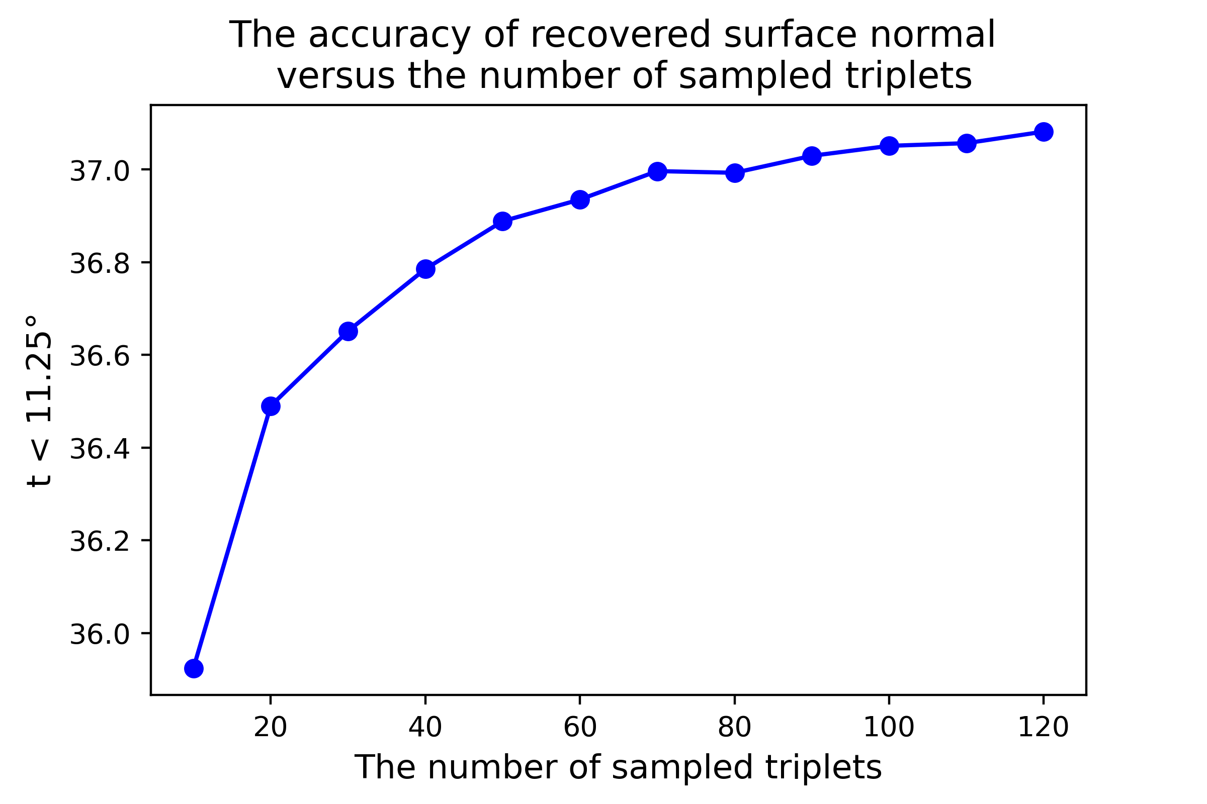
Figure 8: The accuracy of recovered surface normal versus the number of sampled triplets. The more triplets are sampled, the more accurate the recovered surface normal is.

Size of local patch.

We evaluate the effect of the size of local patch to our method by training the network with different local patch sizes. As illustrated in Table 7, a larger local patch could improve the performance, especially for the surface normal, but the improvements are not significant. The reason behind is, our ASN constraint is an adaptive strategy that can automatically determine the reliability of the sampled points given different local patches; therefore, our method is robust to the choice of local patch size.

Table 7: The influence of local patch size.

Size	rel ($\downarrow$)	log10 ($\downarrow$)	$\boldsymbol{\delta_{1}}$ ($\uparrow$)	Mean ($\downarrow$)	Median ($\downarrow$)	$\boldsymbol{11.25^{\circ}}$ ($\uparrow$)
	Depth			Recovered Normal
3	0.112	0.047	0.877	22.5	15.8	36.9
5	0.111	0.047	0.876	22.4	15.8	37.1
7	0.112	0.047	0.877	22.2	15.7	37.1
9	0.111	0.047	0.875	22.4	15.8	37.0

Area-based adaption

We use the area of a sampled triangle as the combinational weight for adaption. To evaluate the effectiveness of the area-based adaption, we conduct an experiment with a comparison to the simple average strategy. We create a unit semi-sphere surface as noise-free data and then add Gaussian noises to simulate real noisy data (see Fig. 9 (a)). We compare the mean of angle errors of the normals estimated by these two methods with the increase of noises, and the results are given in Fig. 9 (b). We can see that our area-based adaption gives lower estimation error with the increase of noise level, demonstrating the robustness of the use of area for adaption.

Time complexity

Here, we discuss the time complexity of different normal computation methods, including our sampling based method, Sobel-like operator [13, 16] and least square based method [28, 26] . Ours and the Sobel-like operator only involve matrix addition and vector dot/cross production operations; thus it is easy to show the time complexity is $O\left(n\right)$, while our time complexity will increase linearly with more samples. However, the least square module [28, 26] directly calculates the closed form solution of least square equations, which involves matrix multiplication, inversion and determinant, leading to the time complexity of $O\left(n^{3}\right)$. Therefore, our method effectively balances the accuracy and computational efficiency.

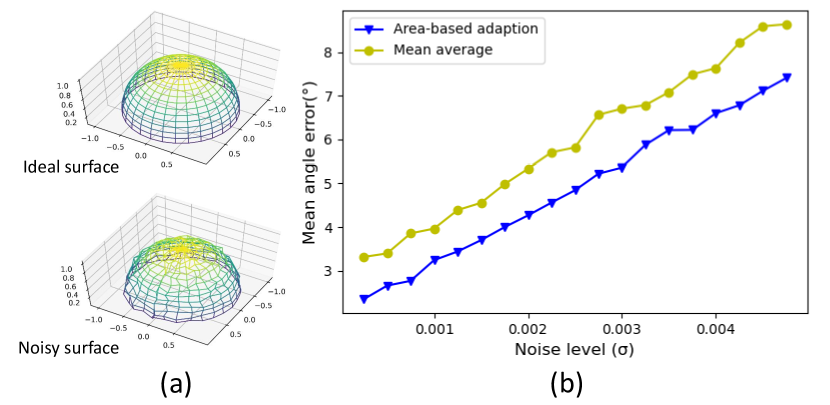
Figure 9: Effectiveness of the area-based adaption. (a) The ideal and noisy surface. (b) We employ the mean angle error to evaluate surface normals estimated by the simple average strategy and our area-based adaption. Compared with the simple average strategy, our area-based adaption is more robust to noises.

6 Conclusion

In this paper, we present a simple but effective Adaptive Surface Normal (ASN) constraint for monocular depth estimation. Compared with other surface normal constraints, our constraint could adaptively determine the reliable local geometry for normal calculation, by jointly leveraging the latent image features and explicit geometry properties. With the geometric constraint, our model not only estimates accurate depth maps but also faithfully preserves important 3D geometric features so that high-quality 3D point clouds and surface normal maps can be recovered from the estimated depth maps.

We thank the anonymous reviewers for their valuable feedback. Wenping Wang acknowledges support from AIR@InnoHK – Center for Transformative Garment Production (TransGP). Christian Theobalt acknowledges support from ERC Consolidator Grant 4DReply (770784). Lingjie Liu acknowledges support from Lise Meitner Postdoctoral Fellowship.

References

- [1] Linchao Bao, Qingxiong Yang, and Hailin Jin. Fast edge-preserving patchmatch for large displacement optical flow. In Proceedings of the IEEE Conference on Computer Vision and Pattern Recognition, pages 3534–3541, 2014.
- [2] Michael J Black, Guillermo Sapiro, David H Marimont, and David Heeger. Robust anisotropic diffusion. IEEE Transactions on image processing, 7(3):421–432, 1998.
- [3] Ayan Chakrabarti, Jingyu Shao, and Gregory Shakhnarovich. Depth from a single image by harmonizing overcomplete local network predictions. arXiv preprint arXiv:1605.07081, 2016.
- [4] Angela Dai, Angel X Chang, Manolis Savva, Maciej Halber, Thomas Funkhouser, and Matthias Nießner. Scannet: Richly-annotated 3d reconstructions of indoor scenes. In Proceedings of the IEEE Conference on Computer Vision and Pattern Recognition, pages 5828–5839, 2017.
- [5] David Eigen and Rob Fergus. Predicting depth, surface normals and semantic labels with a common multi-scale convolutional architecture. In Proceedings of the IEEE international conference on computer vision, pages 2650–2658, 2015.
- [6] David Eigen, Christian Puhrsch, and Rob Fergus. Depth map prediction from a single image using a multi-scale deep network. arXiv preprint arXiv:1406.2283, 2014.
- [7] David F Fouhey, Abhinav Gupta, and Martial Hebert. Data-driven 3d primitives for single image understanding. In Proceedings of the IEEE International Conference on Computer Vision, pages 3392–3399, 2013.
- [8] David Ford Fouhey, Abhinav Gupta, and Martial Hebert. Unfolding an indoor origami world. In European Conference on Computer Vision, pages 687–702. Springer, 2014.
- [9] Huan Fu, Mingming Gong, Chaohui Wang, Kayhan Batmanghelich, and Dacheng Tao. Deep ordinal regression network for monocular depth estimation. In Proceedings of the IEEE Conference on Computer Vision and Pattern Recognition, pages 2002–2011, 2018.
- [10] Clément Godard, Oisin Mac Aodha, and Gabriel J Brostow. Unsupervised monocular depth estimation with left-right consistency. In Proceedings of the IEEE Conference on Computer Vision and Pattern Recognition, pages 270–279, 2017.
- [11] Clément Godard, Oisin Mac Aodha, Michael Firman, and Gabriel J Brostow. Digging into self-supervised monocular depth estimation. In Proceedings of the IEEE/CVF International Conference on Computer Vision, pages 3828–3838, 2019.
- [12] Kaiming He, Xiangyu Zhang, Shaoqing Ren, and Jian Sun. Deep residual learning for image recognition. In Proceedings of the IEEE conference on computer vision and pattern recognition, pages 770–778, 2016.
- [13] Junjie Hu, Mete Ozay, Yan Zhang, and Takayuki Okatani. Revisiting single image depth estimation: Toward higher resolution maps with accurate object boundaries. In 2019 IEEE Winter Conference on Applications of Computer Vision (WACV), pages 1043–1051. IEEE, 2019.
- [14] Jianbo Jiao, Ronggang Wang, Wenmin Wang, Shengfu Dong, Zhenyu Wang, and Wen Gao. Local stereo matching with improved matching cost and disparity refinement. IEEE MultiMedia, 21(4):16–27, 2014.
- [15] Kevin Karsch, Ce Liu, and Sing Bing Kang. Depth extraction from video using non-parametric sampling. In European Conference on Computer Vision, pages 775–788. Springer, 2012.
- [16] Uday Kusupati, Shuo Cheng, Rui Chen, and Hao Su. Normal assisted stereo depth estimation. In Proceedings of the IEEE/CVF Conference on Computer Vision and Pattern Recognition, pages 2189–2199, 2020.
- [17] Lubor Ladicky, Jianbo Shi, and Marc Pollefeys. Pulling things out of perspective. In Proceedings of the IEEE conference on computer vision and pattern recognition, pages 89–96, 2014.
- [18] Iro Laina, Christian Rupprecht, Vasileios Belagiannis, Federico Tombari, and Nassir Navab. Deeper depth prediction with fully convolutional residual networks. In 2016 Fourth international conference on 3D vision (3DV), pages 239–248. IEEE, 2016.
- [19] Jin Han Lee, Myung-Kyu Han, Dong Wook Ko, and Il Hong Suh. From big to small: Multi-scale local planar guidance for monocular depth estimation. arXiv preprint arXiv:1907.10326, 2019.
- [20] Bo Li, Chunhua Shen, Yuchao Dai, Anton Van Den Hengel, and Mingyi He. Depth and surface normal estimation from monocular images using regression on deep features and hierarchical crfs. In Proceedings of the IEEE conference on computer vision and pattern recognition, pages 1119–1127, 2015.
- [21] Jun Li, Reinhard Klein, and Angela Yao. A two-streamed network for estimating fine-scaled depth maps from single rgb images. In Proceedings of the IEEE International Conference on Computer Vision, pages 3372–3380, 2017.
- [22] Fayao Liu, Chunhua Shen, Guosheng Lin, and Ian Reid. Learning depth from single monocular images using deep convolutional neural fields. IEEE transactions on pattern analysis and machine intelligence, 38(10):2024–2039, 2015.
- [23] Lina Liu, Yiyi Liao, Yue Wang, Andreas Geiger, and Yong Liu. Learning steering kernels for guided depth completion. IEEE Transactions on Image Processing, 30:2850–2861, 2021.
- [24] Lina Liu, Xibin Song, Xiaoyang Lyu, Junwei Diao, Mengmeng Wang, Yong Liu, and Liangjun Zhang. Fcfr-net: Feature fusion based coarse-to-fine residual learning for monocular depth completion. arXiv preprint arXiv:2012.08270, 2020.
- [25] Miaomiao Liu, Mathieu Salzmann, and Xuming He. Discrete-continuous depth estimation from a single image. In Proceedings of the IEEE Conference on Computer Vision and Pattern Recognition, pages 716–723, 2014.
- [26] Xiaoxiao Long, Lingjie Liu, Christian Theobalt, and Wenping Wang. Occlusion-aware depth estimation with adaptive normal constraints. In European Conference on Computer Vision, pages 640–657. Springer, 2020.
- [27] Pietro Perona and Jitendra Malik. Scale-space and edge detection using anisotropic diffusion. IEEE Transactions on pattern analysis and machine intelligence, 12(7):629–639, 1990.
- [28] Xiaojuan Qi, Renjie Liao, Zhengzhe Liu, Raquel Urtasun, and Jiaya Jia. Geonet: Geometric neural network for joint depth and surface normal estimation. In Proceedings of the IEEE Conference on Computer Vision and Pattern Recognition, pages 283–291, 2018.
- [29] Xiaojuan Qi, Zhengzhe Liu, Renjie Liao, Philip HS Torr, Raquel Urtasun, and Jiaya Jia. Geonet++: Iterative geometric neural network with edge-aware refinement for joint depth and surface normal estimation. arXiv preprint arXiv:2012.06980, 2020.
- [30] Jiaxiong Qiu, Zhaopeng Cui, Yinda Zhang, Xingdi Zhang, Shuaicheng Liu, Bing Zeng, and Marc Pollefeys. Deeplidar: Deep surface normal guided depth prediction for outdoor scene from sparse lidar data and single color image. In Proceedings of the IEEE/CVF Conference on Computer Vision and Pattern Recognition, pages 3313–3322, 2019.
- [31] Rene Ranftl, Vibhav Vineet, Qifeng Chen, and Vladlen Koltun. Dense monocular depth estimation in complex dynamic scenes. In Proceedings of the IEEE conference on computer vision and pattern recognition, pages 4058–4066, 2016.
- [32] Xiaofeng Ren. Local grouping for optical flow. In 2008 IEEE Conference on Computer Vision and Pattern Recognition, pages 1–8. IEEE, 2008.
- [33] Jerome Revaud, Philippe Weinzaepfel, Zaid Harchaoui, and Cordelia Schmid. Epicflow: Edge-preserving interpolation of correspondences for optical flow. In Proceedings of the IEEE conference on computer vision and pattern recognition, pages 1164–1172, 2015.
- [34] Anirban Roy and Sinisa Todorovic. Monocular depth estimation using neural regression forest. In Proceedings of the IEEE conference on computer vision and pattern recognition, pages 5506–5514, 2016.
- [35] Ashutosh Saxena, Min Sun, and Andrew Y Ng. Make3d: Learning 3d scene structure from a single still image. IEEE transactions on pattern analysis and machine intelligence, 31(5):824–840, 2008.
- [36] Xiao Song, Xu Zhao, Hanwen Hu, and Liangji Fang. Edgestereo: A context integrated residual pyramid network for stereo matching. In Asian Conference on Computer Vision, pages 20–35. Springer, 2018.
- [37] Jingdong Wang, Ke Sun, Tianheng Cheng, Borui Jiang, Chaorui Deng, Yang Zhao, Dong Liu, Yadong Mu, Mingkui Tan, Xinggang Wang, et al. Deep high-resolution representation learning for visual recognition. IEEE transactions on pattern analysis and machine intelligence, 2020.
- [38] Peng Wang, Xiaohui Shen, Zhe Lin, Scott Cohen, Brian Price, and Alan L Yuille. Towards unified depth and semantic prediction from a single image. In Proceedings of the IEEE conference on computer vision and pattern recognition, pages 2800–2809, 2015.
- [39] Xiaolong Wang, David Fouhey, and Abhinav Gupta. Designing deep networks for surface normal estimation. In Proceedings of the IEEE Conference on Computer Vision and Pattern Recognition, pages 539–547, 2015.
- [40] Joachim Weickert. Anisotropic diffusion in image processing, volume 1. Teubner Stuttgart, 1998.
- [41] Jiangjian Xiao, Hui Cheng, Harpreet Sawhney, Cen Rao, and Michael Isnardi. Bilateral filtering-based optical flow estimation with occlusion detection. In European conference on computer vision, pages 211–224. Springer, 2006.
- [42] Dan Xu, Wanli Ouyang, Xiaogang Wang, and Nicu Sebe. Pad-net: Multi-tasks guided prediction-and-distillation network for simultaneous depth estimation and scene parsing. In Proceedings of the IEEE Conference on Computer Vision and Pattern Recognition, pages 675–684, 2018.
- [43] Dan Xu, Elisa Ricci, Wanli Ouyang, Xiaogang Wang, and Nicu Sebe. Multi-scale continuous crfs as sequential deep networks for monocular depth estimation. In Proceedings of the IEEE Conference on Computer Vision and Pattern Recognition, pages 5354–5362, 2017.
- [44] Yan Xu, Xinge Zhu, Jianping Shi, Guofeng Zhang, Hujun Bao, and Hongsheng Li. Depth completion from sparse lidar data with depth-normal constraints. In Proceedings of the IEEE/CVF International Conference on Computer Vision, pages 2811–2820, 2019.
- [45] Zhenheng Yang, Peng Wang, Wei Xu, Liang Zhao, and Ramakant Nevatia. Unsupervised learning of geometry from videos with edge-aware depth-normal consistency. In Proceedings of the AAAI Conference on Artificial Intelligence, volume 32, 2018.
- [46] Wei Yin, Yifan Liu, Chunhua Shen, and Youliang Yan. Enforcing geometric constraints of virtual normal for depth prediction. In Proceedings of the IEEE/CVF International Conference on Computer Vision, pages 5684–5693, 2019.
- [47] Zhenyu Zhang, Zhen Cui, Chunyan Xu, Yan Yan, Nicu Sebe, and Jian Yang. Pattern-affinitive propagation across depth, surface normal and semantic segmentation. In Proceedings of the IEEE/CVF Conference on Computer Vision and Pattern Recognition, pages 4106–4115, 2019.