Self-triggered Stabilization of Discrete-time Linear Systems with Quantized State Measurements

Abstract

We study the self-triggered stabilization of discrete-time linear systems with quantized state measurements. In the networked control system we consider, sensors may be spatially distributed and be connected to a self-triggering mechanism through finite data-rate channels. Each sensor independently encodes its measurements and sends them to the self-triggering mechanism. The self-triggering mechanism integrates quantized measurement data and then computes sampling times. Assuming that the closed-loop system is stable in the absence of quantization and self-triggered sampling, we propose a joint design method of an encoding scheme and a self-triggering mechanism for stabilization. To deal with data inaccuracy due to quantization, the proposed self-triggering mechanism uses not only quantized data but also an upper bound of quantization errors, which is shared with a decoder.

I Introduction

The subject of this note is self-triggered control with quantized state measurements. Quantized control and self-triggered control have been extensively studied in the past few decades. In both research areas, many methods have been developed for control with limited information about plant measurements. However, a synergy between quantized control and self-triggered control has not been studied sufficiently. It is our aim to combine these two research areas. In particular, we construct a self-triggering mechanism that determines sampling times for stabilization from quantized measurements of possibly spatially distributed sensors.

Signal quantization is unavoidable for data transmission over digital communication channels. Coarse quantization may make feedback systems unstable. Moreover, asymptotic convergence to equilibrium points cannot be achieved by static finite-level quantizers in general. Time-varying quantizers for stabilization with finite data rates have been developed in [1, 2]. This class of time-varying quantizers has been introduced for linear time-invariant systems and then has been extended to more general classes of systems such as nonlinear systems [3, 4], switched linear systems [5, 6], and systems under DoS attacks [7]. Instability due to quantization errors raises also a theoretical question of how coarse quantization is allowed without compromising the closed-loop stability. From this motivation, data-rate limitation for stabilization has been extensively investigated; see the surveys [8, 9].

To reduce resource utilization, techniques for aperiodic data transmission have attracted considerable attention. Event-triggered control [10, 11] and self-triggered control [12] are the two major approaches of the aperiodic transmission techniques. In both event-triggered control systems and self-triggered control systems, the transmission of information occurs only when needed. In event-triggered control systems, triggering conditions are based on current measurements and are monitored continuously or periodically. Instead of such frequent monitoring, self-triggering mechanisms compute the next transmission time when they receive measurements. The advantage of self-triggered control systems is that the sensors can be deactivated between transmission times. Various triggering mechanisms, together with stability analysis, have been proposed; see, e.g., [13, 14, 15] for the event-triggered case and [16, 17, 18] for the self-triggered case. Moreover, joint design methods of feedback control laws and triggering mechanisms have been developed in [19, 20, 21, 22] and the references therein.

Quantized event-triggered control has become an active research topic in recent years; see, e.g., [23, 24, 25, 26, 27, 28, 29] and the references therein. However, there has been relatively little work on quantized self-triggered control. A consensus protocol with a quantized self-triggered communication policy has been proposed for multi-agent systems in [30, 31], but these systems differ significantly from the models we study. Sum-of-absolute-values optimization has been employed for self-triggered control with discrete-valued inputs in [32]. In [33], self-triggered and event-triggered control with input and output quantization has been studied. However, the self-triggering mechanisms proposed in [32, 33] need the non-quantized measurements, which would remove difficulties present in the computation of sampling times. Many technical tools are commonly used for quantized control and self-triggered control. This is because analyzing implementation-induced errors plays a crucial role in both research areas. Hence coupling these two research areas is quite natural.

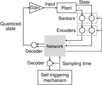
Figure 1: Networked control system. Since the encoding and decoding of sampling times is simple and not essential in our discrete-time setting, we omit it in the figure.

In this note, we consider the networked control system shown in Fig. 1 and assume that the system is stable when no quantization or self-triggering sampling is performed. Our main contribution is to develop a joint design method of an encoding scheme and a self-triggering mechanism for stabilization. The proposed encoding and self-triggering strategy has the following advantageous features:

• The proposed self-triggering mechanism determines sampling times from the quantized state, unlike the self-triggering mechanisms developed in [32, 33] that use the original (non-quantized) state. Due to this property, we do not need to install the self-triggering mechanism at the sensors. Therefore, the proposed encoding and self-triggering strategy is applicable to the scenario in which the sensors do not have computational resources enough to determine sampling times by self-triggering mechanisms; see also [34] for the computational issue of self-triggered control.

• In the proposed encoding scheme, an individual sensor encodes its measurement data without information from other sensors. In contrast, the existing scheme proposed in [33] has to collect measurement data from all sensors in one place. This issue does not arise in the previous study [32] because it considers only input quantization for single-input systems. The distributed architecture allows the proposed encoding scheme to be applied to systems with spatially distributed sensors.

In contrast with the distributed architecture of the encoding scheme, the self-triggering mechanism works in a centralized way, i.e., it integrates measurement data sent by all sensors in order to compute sampling times for stabilization. In this aspect, the use of quantized measurements in the self-triggering mechanism is also important when sensors are spatially distributed. In fact, even when the self-triggering mechanism is colocated with one sensor, it needs to receive measurement data from other distant sensors, which is done through digital channels in most cases.

The quantized self-triggered stabilization problem we study has two difficulties. First, sampling times are computed only from inaccurate information on the plant state. A key insight for solving this issue is that the self-triggering mechanism can share an upper bound of quantization errors with the decoder. To compensate for the inaccuracy of information on the state, the proposed triggering mechanism exploits not only the quantized state but also the upper bound of quantization errors. The second difficulty is that the self-triggered sampling makes the encoding and decoding scheme aperiodic. To deal with this aperiodicity, we introduce in the analysis a new norm with respect to which the closed-loop matrix is a strict contraction. The contraction property of the norm enables us to develop a simple update rule of the encoding and decoding scheme, which requires less computational resources in the encoders.

The remainder of this note is organized as follows. In Section II, the networked control system we consider is introduced. In Section III, we propose a joint design method of an encoding scheme and a self-triggering mechanism for stabilization. We illustrate the proposed method with a numerical example in Section IV and give concluding remarks in Section V.

Notation

The set of non-negative integers and the set of non-negative real numbers are denoted by $\mathbb{N}_{0}$ and $\mathbb{R}_{+}$, respectively. Let $A^{\top}$ be the transpose of a matrix $A\in\mathbb{R}^{m\times n}$. Let $I_{n}$ denote the identity matrix of order $n$. For a vector $v\in\mathbb{R}^{n}$ with $i$th element $v_{i}$, its maximum norm is $\|v\|_{\infty}:=\max\{|v_{i}|,\dots,|v_{n}|\}$. The corresponding induced norm of a matrix $A\in\mathbb{R}^{m\times n}$ with $(i,j)$th element $A_{ij}$ is given by $\|A\|_{\infty}=\max\{\sum_{j=1}^{n}|A_{ij}|:1\leq i\leq m\}$. We denote by $\varrho(P)$ the spectral radius of $P\in\mathbb{R}^{n\times n}$. For a matrix sequence $\{A_{k}\}_{k\in\mathbb{N}_{0}}\subset\mathbb{R}^{m\times n}$, the empty sum $\sum_{k=0}^{-1}A_{k}$ is set to $0$.

II Networked control system

In this section, the control system we consider and a basic encoding and decoding scheme are introduced. We also present the structure of the proposed self-triggering mechanism.

II-A Plant and controller

Consider the discrete-time linear time-invariant system

$$\left\{\begin{aligned} x(k+1)&=Ax(k)+Bu(k),&\qquad&k\in\mathbb{N}_{0},\\ u(k)&=Kq_{\ell},&&k_{\ell}\leq k<k_{\ell+1},\end{aligned}\right.$$ (1)

where $x(k)\in\mathbb{R}^{n}$ and $u(k)\in\mathbb{R}^{m}$ are the state and the input of the plant at time $k\in\mathbb{N}_{0}$, respectively. The time sequence $\{k_{\ell}\}_{\ell\in\mathbb{N}_{0}}$ with $k_{0}:=0$ is computed by a certain self-triggering mechanism, and $q_{\ell}$ is the quantized value of $x(k_{\ell})$.

Define the closed-loop matrix $A_{\text{cl}}$ by $A_{\text{cl}}:=A+BK$. We assume that the closed-loop system is stable in the situation where the state $x(k)$ is transmitted without quantization at all times $k\in\mathbb{N}_{0}$.

Assumption II.1

The feedback gain $K$ is chosen so that the closed-loop matrix $A_{\text{cl}}$ is Schur stable, that is, there exist constants $\Gamma\geq 1$ and $\gamma\in(0,1)$ such that

$$\big{\|}A_{\text{cl}}^{k}\big{\|}_{\infty}\leq\Gamma\gamma^{k}\qquad\forall k\in\mathbb{N}_{0}.$$ (2)

We also place an assumption that a bound of the initial state $x(0)$ is known. One can obtain an initial state bound from the standard zooming-out procedure developed in [2], where quantized signals are assumed to be transmitted at every time.

Assumption II.2

A constant $E_{0}>0$ satisfying $\|x(0)\|_{\infty}\leq E_{0}$ is known.

In this note, we study the following notion of the closed-loop stability.

Definition II.3

The discrete-time system (1) achieves exponential convergence under Assumption II.2 if there exist constants $\Omega\geq 1$ and $\omega\in(0,1)$, independent of $E_{0}$, such that

$$\|x(k)\|_{\infty}\leq\Omega E_{0}\omega^{k}\qquad\forall k\in\mathbb{N}_{0}$$ (3)

for every initial state $x(0)\in\mathbb{R}^{n}$ satisfying $\|x(0)\|_{\infty}\leq E_{0}$.

Remark II.4

Consider the continuous-time linear time-invariant system

$$\dot{x}_{\text{c}}(t)=A_{\text{c}}x_{\text{c}}(t)+B_{\text{c}}u_{\text{c}}(t),\quad t\geq 0,$$ (4)

where $x_{\text{c}}(t)\in\mathbb{R}^{n}$ and $u_{\text{c}}(t)\in\mathbb{R}^{m}$ are the state and the input of the plant at time $t\geq 0$, respectively. A standard self-triggered mechanism is given by

$$t_{\ell+1}:=t_{\ell}+\inf\{\tau>0:f(x(t_{\ell}),\tau)>0\},\quad\ell\in\mathbb{N}_{0}$$

for some function $f:\mathbb{R}^{n}\times\mathbb{R}_{+}\to\mathbb{R}$. However, this mechanism has two implementation issues. First, the next sampling time $t_{\ell+1}$ (or the inter-sampling time $t_{\ell+1}-t_{\ell}$) needs to be quantized when it is sent to the sensors over finite data-rate channels. Second, the triggering mechanism has to check the condition $f(x(k_{\ell}),\tau)>0$ continuously with respect to $\tau>0$. An easy way to circumvent these issues is to place a time-triggering condition $\{t_{\ell}\}_{\ell\in\mathbb{N}_{0}}\subset\{\ell h\}_{\ell\in\mathbb{N}_{0}}$ for some $h>0$ as in the self-triggering mechanism proposed in [18] and the periodic event-triggering mechanism (see, e.g., [15]). When the continuous-time system (4) is discretized with period $h$ under this time-triggering condition, the resulting discrete-time system is in the form (1), where the matrices $A$ and $B$ are given by

$$A=e^{A_{\text{c}}h},\quad B=\int^{h}_{0}e^{A_{\text{c}}\tau}d\tau B_{\text{c}}$$

and the state $x(k)$ and the input $u(k)$ are $x(k)=x_{\text{c}}(kh)$ and $u(k)=u_{\text{c}}(kh)$ for $k\in\mathbb{N}_{0}$.

II-B Basic encoding and decoding scheme

Let $\ell\in\mathbb{N}_{0}$, and assume that we have obtained $E_{\ell}>0$ satisfying $\|x(k_{\ell})\|_{\infty}\leq E_{\ell}$ at the $\ell$th sampling time $k=k_{\ell}$. In the next section, we will explain how to obtain such a bound $E_{\ell}$; see (11) and Lemma III.2 below for details.

Let $\eta\in\mathbb{N}$ be the number of sensors, and let $n_{1},\dots,n_{\eta}\in\mathbb{N}$ satisfy $n=n_{1}+\cdots+n_{\eta}$. We partition the state $x(k_{\ell})$ into

$$x(k_{\ell})=\begin{bmatrix}x^{\langle 1\rangle}(k_{\ell})\\ \vdots\\ x^{\langle\eta\rangle}(k_{\ell})\end{bmatrix},$$

where $x^{\langle i\rangle}(k_{\ell})\in\mathbb{R}^{n_{i}}$ is measured by the $i$th sensor for $i=1,\dots,\eta$. By assumption, $x^{\langle i\rangle}(k_{\ell})$ satisfies $\|x^{\langle i\rangle}(k_{\ell})\|_{\infty}\leq E_{\ell}$. Let $N\in\mathbb{N}$ be the number of quantization levels per dimension. The $i$th encoder divides the hypercube

$$\Big{\{}x^{\langle i\rangle}\in\mathbb{R}^{n_{i}}:\big{\|}x^{\langle i\rangle}\big{\|}_{\infty}\leq E_{\ell}\Big{\}}$$

into $N^{n_{i}}$ equal hypercubes. Indices $\{1,\dots,N^{n_{i}}\}$ are assigned to divided hypercubes by a certain one-to-one mapping. The $i$th encoder sends the index of the divided hypercube containing $x^{\langle i\rangle}(k_{\ell})$ to the decoders at the self-triggering mechanism and the feedback gain. If $x^{\langle i\rangle}(k_{\ell})$ lies on the boundary of several hypercubes, then either one of these hypercubes can be chosen. The decoders calculate the value of the center of the hybercube corresponding the received index, and the quantized value $q_{\ell}^{\langle i\rangle}$ of $x^{\langle i\rangle}(k_{\ell})$ is set to this value. By construction, we obtain

$$\big{\|}q_{\ell}^{\langle i\rangle}-x^{\langle i\rangle}(k_{\ell})\big{\|}_{\infty}\leq\frac{E_{\ell}}{N}.$$ (5)

Define

$$q_{\ell}:=\begin{bmatrix}q_{\ell}^{\langle 1\rangle}\\ \vdots\\ q_{\ell}^{\langle\eta\rangle}\end{bmatrix}\in\mathbb{R}^{n}.$$

Then (5) yields

$$\|q_{\ell}-x(k_{\ell})\|_{\infty}\leq\frac{E_{\ell}}{N}.$$ (6)

II-C Structure of self-triggering mechanism

The sampling times $\{k_{\ell}\}_{\ell\in\mathbb{N}_{0}}$ is generated by a self-triggering mechanism of the form

$$\left\{\begin{aligned} k_{\ell+1}&:=k_{\ell}+\min\{\tau_{\max},~{}\tau_{\ell}\},\quad k_{0}:=0,\\ \tau_{\ell}&:=\min\{\tau\in\mathbb{N}:g(q_{\ell},E_{\ell},\tau)>\sigma E_{\ell}\},\quad\ell\in\mathbb{N}_{0},\end{aligned}\right.$$ (7)

where $\sigma>0$ is a threshold parameter, $\tau_{\max}\in\mathbb{N}$ is an upper bound of inter-sampling times $k_{\ell+1}-k_{\ell}$, that is, $k_{\ell+1}-k_{\ell}\leq\tau_{\max}$ for every $\ell\in\mathbb{N}_{0}$, and $g:\mathbb{R}^{n}\times\mathbb{R}_{+}\times\mathbb{N}_{0}\to\mathbb{R}_{+}$ is a certain function. The details of $g$ will be given in the next section; see (10) below. The self-triggering mechanism (7) determines the next sampling time $k_{\ell+1}$ from the quantized state $q_{\ell}$ and the state bound $E_{\ell}$ without using the original state $x(k_{\ell})$. Therefore, it does not need to be installed at the sensors. Note that the self-triggering mechanism knows from the state bound $E_{\ell}$ that the quantization error does not exceed $E_{\ell}/N$ by (6).

The inter-sampling time $\min\{\tau_{\max},~{}\!\tau_{\ell}\}$ is transmitted to the sensors, and the sensors measure the state at $k_{\ell+1}=k_{\ell}+\min\{\tau_{\max},~{}\!\tau_{\ell}\}$. Setting the upper bound $\tau_{\max}$ allows the self-triggering mechanism to inform the sensors about the next sampling instant with a finite data rate. Since inter-sampling times can be transmitted by a simple encoding and decoding scheme, we omit the details.

In contrast to the distributed encoding scheme described in Section II-B, the sampling times $\{k_{\ell}\}_{\ell\in\mathbb{N}_{0}}$ are computed in a centralized manner, that is, the quantized data from all the sensors are collected in the self-triggering mechanism (7) for the computation of $\{k_{\ell}\}_{\ell\in\mathbb{N}_{0}}$. Individual sensors cannot determine the next sampling time by themselves due to the lack of information on other measurement data (and also of computational resources in some cases). To compute sampling times for stabilization, the centralized self-triggering mechanism (7) integrates measurement data.

III Quantized self-triggered stabilization

The encoding and self-triggering strategy presented in Sections II-B and II-C is completely determined if the following two components are given:

• the sequence $\{E_{\ell}\}_{\ell\in\mathbb{N}_{0}}$ of state bounds for the encoding and decoding scheme;

• the function $g$ in the self-triggering mechanism (7).

In this section, we first construct the function $g$, after analyzing errors due to quantization and self-triggered sampling. Next, we design the sequence $\{E_{\ell}\}_{\ell\in\mathbb{N}_{0}}$ of state bounds under sampling times computed by the self-triggering mechanism (7) with this function $g$. After these preparations, we provide a sufficient condition for the quantized self-triggered control system to achieve exponential convergence. Finally, we summarize the proposed joint design of an encoding scheme and a self-triggering mechanism for stabilization.

III-A Error analysis for self-triggered sampling

We construct the function $g$ in the self-triggering mechanism (7) so that the input error $\|Kq_{\ell}-Kx(k)\|_{\infty}$ satisfies

$$\|Kq_{\ell}-Kx(k)\|_{\infty}\leq\sigma E_{\ell}$$ (8)

for all $k_{\ell}+1\leq k<k_{\ell+1}$ and $\ell\in\mathbb{N}_{0}$. To this end, we first obtain an upper bound of the input error.

Lemma III.1

Let $\ell\in\mathbb{N}_{0}$ and suppose that the system (1) with the encoding and decoding scheme described in Section II-B satisfies $\|x(k_{\ell})\|_{\infty}\leq E_{\ell}$ for some $E_{\ell}>0$. Then the quantized state $q_{\ell}$ satisfies

$$\|Kq_{\ell}-Kx(k)\|_{\infty} \leq\left\|K\left(I_{n}-A^{k-k_{\ell}}-\sum_{\tau=0}^{k-k_{\ell}-1}A^{\tau}BK\right)q_{\ell}\right\|_{\infty}$$

$$\qquad+\big{\|}KA^{k-k_{\ell}}\big{\|}_{\infty}\frac{E_{\ell}}{N}$$ (9)

for all $k_{\ell}\leq k<k_{\ell+1}$.

Proof: Let $\ell\in\mathbb{N}_{0}$ and $k_{\ell}\leq k<k_{\ell+1}$. Since

$$x(k) =A^{k-k_{\ell}}x(k_{\ell})+\sum_{\tau=0}^{k-k_{\ell}-1}A^{\tau}BKq_{\ell}$$

$$=\left(A^{k-k_{\ell}}+\sum_{\tau=0}^{k-k_{\ell}-1}A^{\tau}BK\right)q_{\ell}-A^{k-k_{\ell}}\big{(}q_{\ell}-x(k_{\ell})\big{)},$$

it follows that

$$q_{\ell}-x(k) =\left(I_{n}-A^{k-k_{\ell}}-\sum_{\tau=0}^{k-k_{\ell}-1}A^{\tau}BK\right)q_{\ell}$$

$$\qquad+A^{k-k_{\ell}}\big{(}q_{\ell}-x(k_{\ell})\big{)}.$$

Thus, the inequality (9) follows from (6). $\Box$

We define the function $g$ in the self-triggering mechanism (7) by

$$g(q,E,\tau):=\left\|K\left(I_{n}-A^{\tau}-\sum_{p=0}^{\tau-1}A^{p}BK\right)q\right\|_{\infty}+\big{\|}KA^{\tau}\big{\|}_{\infty}\frac{E}{N}$$ (10)

for $q\in\mathbb{R}^{n}$, $E\geq 0$, and $\tau\in\mathbb{N}_{0}$. Lemma III.1 shows that if $E_{\ell}>0$ satisfies $\|x(k_{\ell})\|_{\infty}\leq E_{\ell}$, then

$$\|Kq_{\ell}-Kx(k)\|_{\infty}\leq g(q_{\ell},E_{\ell},k-k_{\ell})$$

for all $k_{\ell}\leq k<k_{\ell+1}$. Combining this and the triggering condition given in (7), we obtain the desired inequality (8) for all $k_{\ell}+1\leq k<k_{\ell+1}$ and $\ell\in\mathbb{N}_{0}$.

III-B Generating state bounds for encoding-decoding scheme

To complete the design of the encoding and decoding scheme described in Section II-B, we next construct a sequence $\{E_{\ell}\}_{\ell\in\mathbb{N}_{0}}$ satisfying $\|x(k_{\ell})\|_{\infty}\leq E_{\ell}$ for all $\ell\in\mathbb{N}_{0}$. Note that the sampling times $\{k_{\ell}\}_{k\in\mathbb{N}_{0}}$ are computed by the self-triggering mechanism (7) with the function $g$ in (10).

Using the constants $\Gamma\geq 1$ and $\gamma\in(0,1)$ satisfying (2), we define $\{E_{\ell}\}_{\ell\in\mathbb{N}_{0}}$ by

$$\left\{\begin{aligned} E_{\ell}&:=\widetilde{E}_{\ell},\quad\ell\in\mathbb{N},\\ \widetilde{E}_{0}&:=\Gamma E_{0},\\ \widetilde{E}_{\ell+1}&:=\big{(}\gamma^{k_{\ell+1}-k_{\ell}}(1-\delta\sigma)+\delta\sigma\big{)}\widetilde{E}_{\ell},\quad\ell\in\mathbb{N}_{0},\end{aligned}\right.$$ (11)

where

$$\delta:=\frac{\Gamma\|B\|_{\infty}}{1-\gamma}.$$

In the periodic sampling case such as [2, 4, 5, 7], the decay rate of $\{E_{\ell}\}_{\ell\in\mathbb{N}_{0}}$ depends on the number $N$ of quantization levels. However, the update rule (11) uses only the threshold parameter $\sigma$ and the inter-sampling time $k_{\ell+1}-k_{\ell}$. The self-triggering mechanism exploits the advantage of small quantization errors for reducing the number of data transmissions. Consequently, the number $N$ of quantization levels does not directly affect the decay rate of $\{E_{\ell}\}_{\ell\in\mathbb{N}_{0}}$.

The following result provides a simple condition for the hypercube $\{x\in\mathbb{R}^{n}:\|x\|_{\infty}\leq E_{\ell}\}$ to contain the state $x(k_{\ell})$.

Lemma III.2

Suppose that Assumption II.2 hold. Let the time sequence $\{k_{\ell}\}_{\ell\in\mathbb{N}_{0}}$ be as in (7), where the function $g$ is defined by (10). Take a number $N\in\mathbb{N}$ of quantization levels and a thereshold parameter $\sigma>0$ such that

$$\frac{\|K\|_{\infty}}{N}\leq\sigma.$$ (12)

Then the state $x$ of the system (1) satisfies

$$\|x(k_{\ell})\|_{\infty}\leq E_{\ell}\qquad\forall\ell\in\mathbb{N}_{0},$$ (13)

where the sequence $\{E_{\ell}\}_{\ell\in\mathbb{N}_{0}}$ is defined by (11).

To prove this lemma, we use a norm $\|\cdot\|_{\text{cl}}$ with respect to which the closed-loop matrix $A_{\text{cl}}$ is a strict contraction, i.e., $\|A_{\text{cl}}\xi\|_{\text{cl}}<\|\xi\|_{\text{cl}}$ for all nonzero $\xi\in\mathbb{R}^{n}$, under Assumption II.1. Such a norm was constructed for infinite-dimensional systems in [35, Lemma II.1.5] and [36] without detailed proof. We state the finite-dimensional version in the following lemma and include the proof in Appendix for completeness.

Lemma III.3

Let $F\in\mathbb{R}^{n\times n}$, $\Gamma\geq 1$, and $\gamma>0$ satisfy

$$\big{\|}F^{k}\big{\|}_{\infty}\leq\Gamma\gamma^{k}\qquad\forall k\in\mathbb{N}_{0}.$$

Then the function

$${|\kern-1.07639pt|\kern-1.07639pt|\cdot|\kern-1.07639pt|\kern-1.07639pt|} :\mathbb{R}^{n}\to\mathbb{R}$$

$$:\xi\mapsto{|\kern-1.07639pt|\kern-1.07639pt|\xi|\kern-1.07639pt|\kern-1.07639pt|}:=\sup_{k\in\mathbb{N}_{0}}\big{\|}\gamma^{-k}F^{k}\xi\big{\|}_{\infty}$$

is a norm on $\mathbb{R}^{n}$. Moreover, the norm ${|\kern-1.07639pt|\kern-1.07639pt|\cdot|\kern-1.07639pt|\kern-1.07639pt|}$ satisfies

$$\|\xi\|_{\infty}\leq{|\kern-1.07639pt|\kern-1.07639pt|\xi|\kern-1.07639pt|\kern-1.07639pt|}\leq\Gamma\|\xi\|_{\infty}\qquad\forall\xi\in\mathbb{R}^{n}$$ (14)

and

$${\big{|}\kern-1.50696pt\big{|}\kern-1.50696pt\big{|}F^{k}\xi\big{|}\kern-1.50696pt\big{|}\kern-1.50696pt\big{|}}\leq\gamma^{k}{|\kern-1.07639pt|\kern-1.07639pt|\xi|\kern-1.07639pt|\kern-1.07639pt|}\qquad\forall\xi\in\mathbb{R}^{n},~{}\forall k\in\mathbb{N}_{0}.$$ (15)

Under Assumption II.1, there exist constants $\Gamma\geq 1$ and $\gamma\in(0,1)$ such that $\|A_{\text{cl}}^{k}\|_{\infty}\leq\Gamma\gamma^{k}$ for all $k\in\mathbb{N}_{0}$. Using the constants $\Gamma$ and $\gamma$, we define a new norm on $\mathbb{R}^{n}$ by

$$\|\xi\|_{\text{cl}}:=\sup_{k\in\mathbb{N}_{0}}\big{\|}\gamma^{-k}A_{\text{cl}}^{k}\xi\big{\|}_{\infty},\quad\xi\in\mathbb{R}^{n}.$$ (16)

Lemma III.3 shows that the matrix $A_{\text{cl}}$ is a strict contraction with respect to the norm $\|\cdot\|_{\text{cl}}$.

Proof of Lemma III.2: By Lemma III.3, the norm $\|\cdot\|_{\text{cl}}$ defined as in (16) satisfies

$$\|\xi\|_{\infty}\leq\|\xi\|_{\text{cl}}\leq\Gamma\|\xi\|_{\infty}\qquad\forall\xi\in\mathbb{R}^{n}$$ (17)

and

$$\big{\|}A_{\text{cl}}^{k}\xi\big{\|}_{\text{cl}}\leq\gamma^{k}\|\xi\|_{\text{cl}}\qquad\forall\xi\in\mathbb{R}^{n},~{}\forall k\in\mathbb{N}_{0}.$$ (18)

By the property (17), we obtain the desired inequality (13) if

$$\|x(k_{\ell})\|_{\text{cl}}\leq\widetilde{E}_{\ell}\qquad\forall\ell\in\mathbb{N}_{0}.$$ (19)

Using the property (17) and Assumption II.2, we obtain

$$\|x(0)\|_{\text{cl}}\leq\Gamma\|x(0)\|_{\infty}\leq\Gamma E_{0}=\widetilde{E}_{0}.$$

Hence (19) is true for $\ell=0$. We now proceed by induction and assume (19) to be true for some $\ell\in\mathbb{N}_{0}$. Define $e(k):=q_{\ell}-x(k)$ for $k_{\ell}\leq k<k_{\ell+1}$, and set $p_{\ell}:=k_{\ell+1}-k_{\ell}$. Then

$$x(k_{\ell+1})=A_{\text{cl}}^{p_{\ell}}x(k_{\ell})+\sum_{\tau=0}^{p_{\ell}-1}A_{\text{cl}}^{p_{\ell}-\tau-1}BKe(k_{\ell}+\tau).$$ (20)

By (12),

$$g(q_{\ell},E_{\ell},0)=\|K\|_{\infty}\frac{E_{\ell}}{N}\leq\sigma E_{\ell}.$$ (21)

Under the self-triggering mechanism (7), we obtain

$$g(q_{\ell},E_{\ell},\tau)\leq\sigma E_{\ell}$$ (22)

for all $1\leq\tau<p_{\ell}$. By definition, $E_{\ell}=\widetilde{E}_{\ell}$ for all $\ell\in\mathbb{N}$ and $E_{\ell}\leq\Gamma E_{\ell}=\widetilde{E}_{\ell}$ for $\ell=0$. Since $\|x(k_{\ell})\|_{\infty}\leq E_{\ell}$ by assumption, Lemma III.1 in the combination with the inequalities (21) and (22) yields

$$\|Ke(k_{\ell}+\tau)\|_{\infty}\leq g(q_{\ell},E_{\ell},\tau)\leq\sigma E_{\ell}\leq\sigma\widetilde{E}_{\ell}$$

for all $0\leq\tau<p_{\ell}$. Applying the properties (17) and (18) to (20), we obtain

$$\|x(k_{\ell+1})\|_{\text{cl}}$$

$$\quad\leq\gamma^{p_{\ell}}\|x(k_{\ell})\|_{\text{cl}}+\Gamma\sum_{\tau=0}^{p_{\ell}-1}\gamma^{p_{\ell}-\tau-1}\|B\|_{\infty}\|Ke(k_{\ell}+\tau)\|_{\infty}$$

$$\quad\leq\gamma^{p_{\ell}}\widetilde{E}_{\ell}+\sigma\Gamma\|B\|_{\infty}\sum_{\tau=0}^{p_{\ell}-1}\gamma^{\tau}\widetilde{E}_{\ell}$$

$$\quad\leq\big{(}\gamma^{p_{\ell}}(1-\delta\sigma)+\delta\sigma\big{)}\widetilde{E}_{\ell}=\widetilde{E}_{\ell+1}.$$ (23)

Thus, (19) holds for $\ell+1$. $\blacksquare$

III-C Sufficient condition for exponential convergence

The following theorem gives a sufficient condition for the closed-loop system to achieve exponential convergence.

Theorem III.4

Suppose that Assumptions II.1 and II.2 hold. Construct the components $g$ and $\{E_{\ell}\}_{\ell\in\mathbb{N}_{0}}$ of the encoding and self-triggering strategy by (10) and (11), respectively. If the number $N\in\mathbb{N}$ of quantization levels and the thereshold parameter $\sigma>0$ satisfy

$$\frac{\|K\|_{\infty}}{N}\leq\sigma<\frac{1}{\delta}=\frac{1-\gamma}{\Gamma\|B\|_{\infty}},$$ (24)

then the system (1) with the encoding and self-triggering strategy described in Sections II-B and II-C achieves exponential convergence. Moreover, the constant $\omega$ given by

$$\omega:=\big{(}\gamma^{\tau_{\max}}(1-\delta\sigma)+\delta\sigma\big{)}^{1/\tau_{\max}}$$ (25)

satisfies (3) for some $\Omega\geq 1$.

Before proceeding to the proof of this theorem, we provide some remarks on the obtained sufficient condition (24). The condition $\|K\|_{\infty}/N\leq\sigma$ is used to avoid $g(q_{\ell},E_{\ell},0)>\sigma E_{\ell}$ for $\ell\in\mathbb{N}_{0}$ as shown in the proof of Lemma III.2; see (21). Without this condition, the input error due to quantization may be larger than the threshold $\sigma E_{\ell}$ even at the sampling time $k=k_{\ell}$. On the other hand, the condition $\sigma<1/\delta$ is used to guarantee exponential convergence. In fact, we see from the definition (11) of $\{E_{\ell}\}_{\ell\in\mathbb{N}_{0}}$ that the condition $\sigma<1/\delta$ is satisfied if and only if $\{E_{\ell}\}_{\ell\in\mathbb{N}_{0}}$ is a decreasing sequence. Combing this fact with the bound of the state obtained in (13), we prove that the closed-loop system achieves exponential convergence.

Proof of Theorem III.4: Since $\delta\sigma<1$ by (24), it follows that

$$\gamma^{\tau}(1-\delta\sigma)+\delta\sigma<\gamma^{0}(1-\delta\sigma)+\delta\sigma=1\qquad\forall\tau\in\mathbb{N}.$$

Define

$$\omega:=\max_{1\leq\tau\leq\tau_{\max}}\big{(}\gamma^{\tau}(1-\delta\sigma)+\delta\sigma\big{)}^{1/\tau}<1.$$

By the definition (11) of $\{E_{\ell}\}_{\ell\in\mathbb{N}_{0}}$,

$$\widetilde{E}_{\ell+1}\leq\widetilde{E}_{\ell}\omega^{k_{\ell+1}-k_{\ell}}\qquad\forall\ell\in\mathbb{N}_{0}.$$

Therefore

$$E_{\ell}\leq\widetilde{E}_{\ell}\leq\widetilde{E}_{0}\omega^{k_{\ell}}=\Gamma E_{0}\omega^{k_{\ell}}\qquad\forall\ell\in\mathbb{N}_{0}.$$ (26)

For all $k_{\ell}\leq k<k_{\ell+1}$ and $\ell\in\mathbb{N}_{0}$,

$$x(k)=A^{k-k_{\ell}}x(k_{\ell})+\sum_{\tau=0}^{k-k_{\ell}-1}A^{\tau}BKq_{\ell}.$$

Lemma III.2 gives

$$\|x(k_{\ell})\|_{\infty}\leq E_{\ell}\qquad\forall\ell\in\mathbb{N}_{0},$$

and by construction, the quantized value $q_{\ell}$ also satisfies

$$\|q_{\ell}\|_{\infty}\leq E_{\ell}\qquad\forall\ell\in\mathbb{N}_{0}.$$

Therefore, there exists $M\geq 1$ such that for all $k_{\ell}\leq k<k_{\ell+1}$ and $\ell\in\mathbb{N}_{0}$,

$$\|x(k)\|_{\infty}\leq ME_{\ell}.$$

Combining this with (26), we obtain

$$\|x(k)\|_{\infty} \leq(M\Gamma)E_{0}\omega^{k_{\ell}}$$

$$\leq\big{(}\omega^{-\tau_{\max}}M\Gamma\big{)}E_{0}\omega^{k}$$

for all $k_{\ell}\leq k<k_{\ell+1}$ and $\ell\in\mathbb{N}_{0}$. Thus, the system (1) achieves exponential convergence.

It remains to show that

$$\tau_{\max}=\mathop{\rm arg\hskip 2.0ptmax}_{1\leq\tau\leq\tau_{\max}}\big{(}\gamma^{\tau}(1-\delta\sigma)+\delta\sigma\big{)}^{1/\tau}.$$ (27)

This fact was used in Theorem 5.8 of [36] without proof. Here we give all details for the sake of completeness.

We prove that

$$\phi(\tau):=\big{(}\gamma^{\tau}(1-\delta\sigma)+\delta\sigma\big{)}^{1/\tau}$$

is strictly increasing on $[1,\infty)$. It suffices to show that

$$\Phi(\tau):=\log\phi(\tau)=\frac{\log(\gamma^{\tau}(1-\delta\sigma)+\delta\sigma)}{\tau}$$

satisfies $\Phi^{\prime}(\tau)>0$ for every $\tau>0$. Define

$$\nu(\tau):=\gamma^{\tau}(1-\delta\sigma)+\delta\sigma.$$

Since

$$\Phi^{\prime}(\tau)=\frac{\frac{\nu^{\prime}(\tau)}{\nu(\tau)}\tau-\log\nu(\tau)}{\tau^{2}},$$

it follows that $\Phi^{\prime}(\tau)>0$ if and only if

$$\psi(\tau):=\frac{\nu^{\prime}(\tau)}{\nu(\tau)}\tau-\log\nu(\tau)>0.$$

We have that

$$\psi^{\prime}(\tau)=\frac{\tau\big{(}\nu(\tau)\nu^{\prime\prime}(\tau)-\nu^{\prime}(\tau)^{2}\big{)}}{\nu(\tau)^{2}}$$

for all $\tau>0$. Therefore, $\psi^{\prime}(\tau)>0$ if and only if

$$\ \nu(\tau)\nu^{\prime\prime}(\tau)-\nu^{\prime}(\tau)^{2}>0.$$

Since

$$\nu^{\prime}(\tau) =\gamma^{\tau}(1-\delta\sigma)\log\gamma$$

$$\nu^{\prime\prime}(\tau) =\gamma^{\tau}(1-\delta\sigma)(\log\gamma)^{2},$$

it follows from $0<\delta\sigma<1$ that

$$\nu(\tau)\nu^{\prime\prime}(\tau)-\nu^{\prime}(\tau)^{2}=\gamma^{\tau}\delta\sigma(1-\delta\sigma)(\log\gamma)^{2}>0$$

for all $\tau>0$. Therefore, $\psi^{\prime}(\tau)>0$. Since $\psi(0)=0$, we obtain $\psi(\tau)>0$ and hence $\Phi^{\prime}(\tau)>0$ for all $\tau>0$. Thus, (27) holds. $\blacksquare$

III-D Design of encoding and self-triggering strategy

Based on Theorem III.4, we design an encoding and self-triggering strategy for stabilization. Before doing so, we explain how to compute constants $\Gamma\geq 1$ and $\gamma\in(0,1)$ satisfying (2). First, we set a constant $\gamma\in(0,1)$. Next, we numerically compute a constant $\Gamma\geq 1$ corresponding to $\gamma$ as

$$\Gamma=\sup_{k\in\mathbb{N}_{0}}\big{\|}\gamma^{-k}A_{\text{cl}}^{k}\big{\|}_{\infty}.$$ (28)

Let $\varrho(A_{\text{cl}})$ be the spectral radius of $A_{\text{cl}}$. Every $\gamma>\varrho(A_{\text{cl}})$ satisfies (2) for some $\Gamma\geq 1$. On the other hand, if $\gamma<\varrho(A_{\text{cl}})$, there does not exist a constant $\Gamma\geq 0$ such that (2) holds. Note that a smaller $\gamma$ does not always allow a larger threshold parameter $\sigma$, because the constant $\Gamma$ given by (28) becomes larger as $\gamma$ decreases.

We summarize the proposed joint design of an encoding scheme and a self-triggering mechanism for exponential convergence.

Encoding and self-triggering strategy

• Take an upper bound $\tau_{\max}$ of inter-sampling times and a decay parameter $\gamma\in(\varrho(A_{\text{cl}}),1)$. Set $\Gamma:=\sup_{k\in\mathbb{N}_{0}}\|\gamma^{-k}A_{\text{cl}}^{k}\|_{\infty}$, and choose a number $N\in\mathbb{N}$ of quantization levels and a threshold parameter $\sigma>0$ so that

  $$\frac{\|K\|_{\infty}}{N}\leq\sigma<\frac{1-\gamma}{\Gamma\|B\|_{\infty}}.$$ (29)

At each sampling time $k_{\ell}$, the following information flow and computation occur.

• The encoders generate the indices corresponding to the state $x(k_{\ell})$ by the scheme described in Section II-B and then transmit them to the self-triggering mechanism and the feedback gain. At both components, the indices are decoded to the quantized value $q_{\ell}$ of $x(k_{\ell})$.

• The inter-sampling time $k_{\ell+1}-k_{\ell}\in\{1,\dots,\tau_{\max}\}$ is computed by the self-triggering mechanism (7), where the function $g$ is given by (10), and then is sent to the sensors, the encoders, and the decoders.

• The encoders at the sensors calculate the next state bound $E_{\ell+1}$ by the update rule (11). The decoders at the self-triggering mechanism and the feedback gain also perform the same calculation.

We make some comments on the above strategy. First, in Step 2, the inter-sample time $k_{\ell+1}-k_{\ell}$ is transmitted to the encoders and the decoders. This is because they also utilize inter-sampling times in Step 3 for the computation of the next state bound $E_{\ell+1}$. Second, the distributed architecture described in Section II-B and the update rule (11) of $\{E_{\ell}\}_{\ell\in\mathbb{N}_{0}}$ allow each sensor to encode its own measurements without using the measurements of the other sensors. Hence, the proposed strategy can be applied to the system whose sensors are spatially distributed.

We immediately see that the condition (29) holds for every sufficiently large number $N\in\mathbb{N}$ of quantization levels and every sufficiently small threshold parameter $\sigma>0$. In other words, the closed-loop system achieves exponential convergence under sufficiently fine quantization and fast self-triggered sampling. Whether exponential convergence is achieved does not depend on the upper bound $\tau_{\max}$ of inter-sampling times, but the upper bound $\omega$ of the decay rate of the state given in (25) becomes smaller as $\tau_{\max}$ increases. Note that $\omega$ depends on $\sigma$ but not on $N$. Fine quantization reduces the number of data transmissions in the proposed encoding and self-triggering strategy, but $\omega$ is determined only by the parameters of self-triggered sampling.

Remark III.5

Proposition 3.13 of [7] provides another method to construct a norm with respect to which $A_{\text{cl}}$ is a strict contraction under Assumption II.1. In this method, an invertible matrix is a design parameter for the encoding and decoding scheme. Since a decay parameter $\gamma$ is easier to tune than an invertible matrix, we here use Lemma III.3 for the construction of a new norm.

IV Numerical Example

We discretize the linearized model of the unstable batch reactor studied in [37] with sampling period $h=0.01$. Then the matrices $A$ and $B$ in the state equation (1) are given by

$$A =\begin{bmatrix}1.0142&-0.0018&0.0651&-0.0546\\ -0.0057&0.9582&-0.0001&0.0067\\ 0.0103&0.0417&0.9363&0.0563\\ 0.0004&0.0417&0.0129&0.9797\end{bmatrix}$$

$$B =10^{-2}\times\begin{bmatrix}0.0005&-0.1034\\ 5.5629&0.0002\\ 1.2511&-3.0444\\ 1.2511&-0.0205\end{bmatrix}.$$

For this discretized system, we compute the linear quadratic regulator whose state weighting matrix and input weighting matrix are the diagonal matrices $I_{4}$ and $0.05\times I_{2}$, respectively. The resulting feedback gain $K$ is given by

$$K=\begin{bmatrix}1.3565&-3.3445&-0.5501&-3.8646\\ 5.8856&-0.0462&4.5150&-2.4334\end{bmatrix}.$$

The closed-loop matrix $A_{\text{cl}}=A+BK$ is Schur stable, and Assumption II.1 is satisfied. For the computation of time responses, we take the initial state

$$x(0)=\begin{bmatrix}-1&-1&-1&1\end{bmatrix}^{\top}.$$

The initial state bound $E_{0}$ in Assumption II.2 is set to $1.1$.

The spectral radius of the closed-loop matrix $A_{\text{cl}}$ is given by $\varrho(A_{\text{cl}})=0.9402$, and we set $\gamma=1.01\times\varrho(A_{\text{cl}})=0.9496$. Then $\Gamma$ defined by (28) is $\Gamma=2.6012$. By Theorem III.4, if the number $N$ of quantization levels and the threshold parameter $\sigma$ satisfy

$$\frac{12.8803}{N}\leq\sigma<0.3482,$$ (30)

then the closed-loop system achieves exponential convergence. The parameters of the self-triggering mechanism are given by $\sigma=0.28$ and $\tau_{\max}=20$, and we consider two cases $N=61$ and $N=101$. The condition (30) is satisfied in both cases. In what follows, we compare the time responses between the cases $N=61$ and $N=101$.

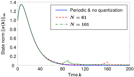
Figure 2: State norm $\|x(k)\|_{\infty}$.

Fig. 2 shows the time responses of the state norm $\|x(k)\|_{\infty}$. The blue solid line shows the ideal case where the state $x(k)$ is transmitted at every $k\in\mathbb{N}_{0}$ without quantization. The red dashed line and the green dotted line indicate the cases $N=61$ and $N=101$, respectively. We see from Fig. 2 that the state norm converges to zero in both cases. The convergence speeds have little difference between the cases $N=61$ and $N=101$, although quantization errors become smaller as $N$ increases. This is because $N$ is related to the number of data transmissions rather than the convergence speed.

To see this, we plot the inter-sampling times $k_{\ell+1}-k_{\ell}$ for the cases $N=61$ and $N=101$ in Figs. 3(a) and 3(b), respectively. We see from these figures that the inter-sampling times in the case $N=101$ are larger than those in the case $N=61$. In particular, the number of data transmissions for $k\geq 40$ is significantly reduced by the self-triggering mechanism in the case $N=101$. The total numbers of data transmissions in the time-interval $[0,200]$ are $62$ for the case $N=61$ and $37$ for the case $N=101$. The amount of data per transmission in the case $N=101$ is $(101/61)^{4}=7.5156$ times larger than that in the case $N=61$. Hence the total amount of transmitted data in the time-interval $[0,200]$ for the case $N=61$ is smaller than that for the case $N=101$. Note, however, that an important benefit to be gained from fine quantization is that the sensors can save energy and extend their lifetime, by reducing the number of sampling.

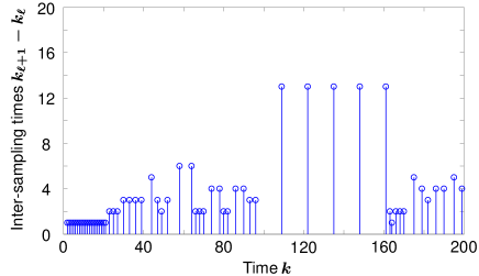
(a) Case $N=61$.

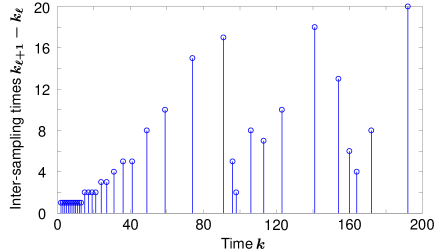
(b) Case $N=101$.

Figure 3: Inter-sampling times $k_{\ell+1}-k_{\ell}$.

Fig. 4 plots the sequence $\{E_{\ell}\}_{\ell\in\mathbb{N}_{0}}$ of state bounds used for the encoding and decoding scheme. The blue circles and the red squares indicate the cases $N=61$ and $N=101$, respectively. In both cases, $\{E_{\ell}\}_{\ell\in\mathbb{N}_{0}}$ converges to zero; see also (26). We have shown in the proof of Theorem III.4 that the decay rate

$$\big{(}\gamma^{k_{\ell+1}-k_{\ell}}(1-\delta\sigma)+\delta\sigma\big{)}^{\frac{1}{k_{\ell+1}-k_{\ell}}}$$

in the update rule (11) becomes smaller as the inter-sampling time $k_{\ell+1}-k_{\ell}$ increases. Since the inter-sampling times in the case $N=101$ are large compared with those in the case $N=61$ as seen in Figs. 3(a) and 3(b), the convergence speed of the red squires ($N=101$) is slightly slower than that of the blue circles ($N=61$) in Fig. 4.

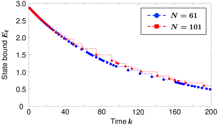
Figure 4: State bound $E_{\ell}$.

Figs. 5(a) and 5(b) show the time responses of the first element $x^{\langle 1\rangle}(k)\in\mathbb{R}$ of the state $x(k)$ and its quantized value $q^{\langle 1\rangle}_{\ell}$ in the cases $N=61$ and $N=101$, respectively. The average values of the quantization errors are given by $1.2523\times 10^{-2}$ in the case $N=61$ and $9.6675\times 10^{-3}$ in the case $N=101$. As expected, the quantization errors in the case $N=101$ are smaller on average than those in the case $N=61$. We see from Figs. 5(a) and 5(b) that the accurate information on the state due to fine quantization is utilized to reduce the number of data transmissions.

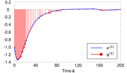
(a) Case $N=61$.

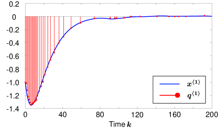
(b) Case $N=101$.

Figure 5: State $x^{\langle 1\rangle}$ and quantized value $q^{\langle 1\rangle}$.

V Conclusion

We have developed a joint strategy of encoding and self-triggered sampling for the stabilization of discrete-time linear systems. The encoding method is distributed in the sense that an individual sensor encodes its measurements without knowing measurement data of other sensors. To compute sampling times, the centralized self-triggering mechanism integrates quantized measurement data sent from possibly spatially distributed sensors and then estimates input errors due to quantization and self-triggered sampling. We have provided a sufficient condition for the stabilization of the quantized self-triggered control system. This sufficient condition is described by inequalities on the number of quantization levels and the threshold parameter of the self-triggering mechanism. Future work involves extending the proposed method to output feedback stabilization in the presence of disturbances and guaranteed cost control.

Appendix

Proof of Lemma III.3

First we show that the map ${|\kern-1.07639pt|\kern-1.07639pt|\cdot|\kern-1.07639pt|\kern-1.07639pt|}$ is a norm on $\mathbb{R}^{n}$. Since

$$\big{\|}\gamma^{-k}F^{k}\xi\big{\|}_{\infty}\leq\gamma^{-k}\Gamma\gamma^{k}\|\xi\|_{\infty}\leq\Gamma\|\xi\|_{\infty}$$ (31)

for all $k\in\mathbb{N}_{0}$ and $\xi\in\mathbb{R}^{n}$, it follows that ${|\kern-1.07639pt|\kern-1.07639pt|\xi|\kern-1.07639pt|\kern-1.07639pt|}<\infty$ for all $\xi\in\mathbb{R}^{n}$.

By definition, ${|\kern-1.07639pt|\kern-1.07639pt|\xi|\kern-1.07639pt|\kern-1.07639pt|}\geq 0$ for every $\xi\in\mathbb{R}^{n}$ and ${|\kern-1.07639pt|\kern-1.07639pt|0|\kern-1.07639pt|\kern-1.07639pt|}=0$. Since

$$\|\xi\|_{\infty}=\big{\|}\gamma^{-0}F^{0}\xi\big{\|}_{\infty}\leq\sup_{k\in\mathbb{N}_{0}}\big{\|}\gamma^{-k}F^{k}\xi\big{\|}={|\kern-1.07639pt|\kern-1.07639pt|\xi|\kern-1.07639pt|\kern-1.07639pt|}$$ (32)

for every $\xi\in\mathbb{R}^{n}$, it follows that ${|\kern-1.07639pt|\kern-1.07639pt|\xi|\kern-1.07639pt|\kern-1.07639pt|}=0$ implies $\xi=0$. For all $a\in\mathbb{R}$ and $\xi\in\mathbb{R}^{n}$,

$${|\kern-1.07639pt|\kern-1.07639pt|a\xi|\kern-1.07639pt|\kern-1.07639pt|} =\sup_{k\in\mathbb{N}_{0}}\big{\|}\gamma^{-k}F^{k}(a\xi)\big{\|}_{\infty}$$

$$=|a|\sup_{k\in\mathbb{N}_{0}}\big{\|}\gamma^{-k}F^{k}\xi\big{\|}_{\infty}$$

$$=|a|~{}\!{|\kern-1.07639pt|\kern-1.07639pt|\xi|\kern-1.07639pt|\kern-1.07639pt|}.$$

For every $\xi,\zeta\in\mathbb{R}^{n}$,

$${|\kern-1.07639pt|\kern-1.07639pt|\xi+\zeta|\kern-1.07639pt|\kern-1.07639pt|} =\sup_{k\in\mathbb{N}_{0}}\big{\|}\gamma^{-k}F^{k}(\xi+\zeta)\big{\|}_{\infty}$$

$$\leq\sup_{k\in\mathbb{N}_{0}}\big{(}\big{\|}\gamma^{-k}F^{k}\xi\big{\|}_{\infty}+\big{\|}\gamma^{-k}F^{k}\zeta\big{\|}_{\infty}\big{)}$$

$$\leq\sup_{k\in\mathbb{N}_{0}}\big{\|}\gamma^{-k}F^{k}\xi\big{\|}_{\infty}+\sup_{k\in\mathbb{N}_{0}}\big{\|}\gamma^{-k}F^{k}\zeta\big{\|}_{\infty}$$

$$={|\kern-1.07639pt|\kern-1.07639pt|\xi|\kern-1.07639pt|\kern-1.07639pt|}+{|\kern-1.07639pt|\kern-1.07639pt|\zeta|\kern-1.07639pt|\kern-1.07639pt|}.$$

Thus, ${|\kern-1.07639pt|\kern-1.07639pt|\cdot|\kern-1.07639pt|\kern-1.07639pt|}$ is a norm on $\mathbb{R}^{n}$.

Next we prove that the norm ${|\kern-1.07639pt|\kern-1.07639pt|\cdot|\kern-1.07639pt|\kern-1.07639pt|}$ has the properties (14) and (15). Take $\xi\in\mathbb{R}^{n}$. We have already shown in (32) that $\|\xi\|_{\infty}\leq{|\kern-1.07639pt|\kern-1.07639pt|\xi|\kern-1.07639pt|\kern-1.07639pt|}$. On the other hand, (31) yields

$${|\kern-1.07639pt|\kern-1.07639pt|\xi|\kern-1.07639pt|\kern-1.07639pt|}=\sup_{k\in\mathbb{N}_{0}}\big{\|}\gamma^{-k}F^{k}\xi\big{\|}\leq\Gamma\|\xi\|_{\infty}.$$

Therefore, (14) holds. The remaining assertion (15) follows by

$${\big{|}\kern-1.50696pt\big{|}\kern-1.50696pt\big{|}F^{k}\xi\big{|}\kern-1.50696pt\big{|}\kern-1.50696pt\big{|}} =\sup_{\ell\in\mathbb{N}_{0}}\big{\|}\gamma^{-\ell}F^{k+\ell}\xi\big{\|}$$

$$=\gamma^{k}\sup_{\ell\in\mathbb{N}_{0}}\big{\|}\gamma^{-(k+\ell)}F^{k+\ell}\xi\big{\|}$$

$$\leq\gamma^{k}{|\kern-1.07639pt|\kern-1.07639pt|\xi|\kern-1.07639pt|\kern-1.07639pt|}\qquad\forall k\in\mathbb{N}_{0}.$$

This completes the proof. $\blacksquare$

References

- [1] R. W. Brockett and D. Liberzon, “Quantized feedback stabilization of linear systems,” IEEE Trans. Automat. Control, vol. 45, pp. 1279–1289, 2000.
- [2] D. Liberzon, “On stabilization of linear systems with limited information,” IEEE Trans. Automat. Control, vol. 48, pp. 304–307, 2003.
- [3] ——, “Hybrid feedback stabilization of systems with quantized signals,” Automatica, vol. 39, pp. 1543–1554, 2003.
- [4] D. Liberzon and J. P. Hespanha, “Stabilization of nonlinear systems with limited information feedback,” IEEE Trans. Automat. Control, vol. 50, pp. 910–915, 2005.
- [5] D. Liberzon, “Finite data-rate feedback stabilization of switched and hybrid linear systems,” Automatica, vol. 50, pp. 409–420, 2014.
- [6] M. Wakaiki and Y. Yamamoto, “Stabilization of switched linear systems with quantized output and switching delays,” IEEE Trans. Automat. Control, vol. 62, pp. 2958–2964, 2017.
- [7] M. Wakaiki, A. Cetinkaya, and H. Ishii, “Stabilization of networked control systems under DoS attacks and output quantization,” IEEE Trans. Automat. Control, vol. 65, pp. 3560–3575, 2020.
- [8] G. N. Nair, F. Fagnani, S. Zampieri, and R. J. Evans, “Feedback control under data rate constraints: An overview,” Proc. IEEE, vol. 95, pp. 108–137, 2007.
- [9] H. Ishii and K. Tsumura, “Data rate limitations in feedback control over networks,” IEICE Trans. Fundamentals, vol. E95-A, pp. 680–690, 2012.
- [10] K.-E. Årzén, “A simple event-based PID controller,” in Proc. 14th IFAC WC, 1999.
- [11] K. J. Åström and B. M. Bernhardsson, “Comparison of Riemann and Lebesgue sampling for first order stochastic systems,” in Proc. 41st CDC, 2002.
- [12] M. Velasco, J. Fuertes, and P. Marti, “The self triggered task model for real-time control systems,” in Proc. 24th IEEE Real-Time Systems Symposium, Work-in-Progress Session, 2003.
- [13] P. Tabuada, “Event-triggered real-time scheduling of stabilizing control tasks,” IEEE Trans. Automat. Control, vol. 52, pp. 1680–1685, 2007.
- [14] W. P. M. H. Heemels, J. Sandee, and P. van den Bosch, “Analysis of event-driven controllers for linear systems,” Int. J. Control, vol. 81, pp. 571–590, 2008.
- [15] W. P. M. H. Heemels, M. C. F. Donkers, and A. R. Teel, “Periodic event-triggered control for linear systems,” IEEE Trans. Automat. Control, vol. 58, pp. 847–861, 2013.
- [16] X. Wang and M. D. Lemmon, “Self-triggered feedback control systems with finite-gain stability,” IEEE Trans. Automat. Control, vol. 54, pp. 452–467, 2009.
- [17] A. Anta and P. Tabuada, “To sample or not to sample: Self-triggered control for nonlinear systems,” IEEE Trans. Automat. Control, vol. 55, pp. 2030–2042, 2010.
- [18] M. Mazo, A. Anta, and P. Tabuada, “An ISS self-triggered implementation of linear controllers,” Automatica, vol. 46, pp. 1310–1314, 2010.
- [19] M. Ghodrat and H. J. Marquez, “On the event-triggered controller design,” IEEE Trans. Automat. Control, vol. 65, pp. 4122–4137, 2020.
- [20] M. Xue, H. Yan, H. Zhang, Z. Li, S. Chen, and C. Chen, “Event-triggered guaranteed cost controller design for T-S fuzzy Markovian jump systems with partly unknown transition probabilities,” IEEE Trans. Fuzzy Systems, vol. 29, pp. 1052–1064, 2021.
- [21] L. Lu and J. M. Maciejowski, “Self-triggered MPC with performance guarantee using relaxed dynamic programming,” Automatica, vol. 114, Art. no. 108803, 2020.
- [22] H. Wan, X. Luan, H. R. Karimi, and F. Liu, “Dynamic self-triggered controller codesign for Markov jump systems,” IEEE Trans. Automat. Control, vol. 66, pp. 1353–1360, 2021.
- [23] E. Garcia and P. J. Antsaklis, “Model-based event-triggered control for systems with quantization and time-varying network delays,” IEEE Trans. Automat. Control, vol. 58, pp. 422–434, 2013.
- [24] L. Li, X. Wang, and M. D. Lemmon, “Efficiently attentive event-triggered systems with limited bandwidth,” IEEE Trans. Automat. Control, vol. 62, pp. 1491–1497, 2016.
- [25] A. Tanwani, C. Prieur, and M. Fiacchini, “Observer-based feedback stabilization of linear systems with event-triggered sampling and dynamic quantization,” Systems Control Lett., vol. 94, pp. 46–56, 2016.
- [26] D. Du, B. Qi, M. Fei, and Z. Wang, “Quantized control of distributed event-triggered networked control systems with hybrid wired–wireless networks communication constraints,” Inf. Sci., vol. 380, pp. 74–91, 2017.
- [27] T. Liu and Z.-P. Jiang, “Event-triggered control of nonlinear systems with state quantization,” IEEE Trans. Automat. Control, vol. 64, pp. 797–803, 2018.
- [28] M. Abdelrahim, V. S. Dolk, and W. P. M. H. Heemels, “Event-triggered quantized control for input-to-state stabilization of linear systems with distributed output sensors,” IEEE Trans. Automat. Control, vol. 64, pp. 4952–4967, 2019.
- [29] G. Wang, “Event-triggered scheduling control for linear systems with quantization and time-delay,” Eur. J. Control, vol. 58, pp. 168–173, 2021.
- [30] C. De Persis and P. Frasca, “Robust self-triggered coordination with ternary controllers,” IEEE Trans. Automat. Control, vol. 58, pp. 3024–3038, 2013.
- [31] H. Matsume, Y. Wang, and H. Ishii, “Resilient self/event-triggered consensus based on ternary control,” Nonlinear Anal.: Hybrid Systems, vol. 42, Art. no. 101091, 2021.
- [32] T. Ikeda, M. Nagahara, and D. E. Quevedo, “Quantized self-triggered control by sum-of-absolute-values optimization,” in Proc. MTNS 2016, 2016.
- [33] T. Zhou, Z. Zuo, and Y. Wang, “Self-triggered and event-triggered control for linear systems with quantization,” IEEE Trans. System, Man, Cybern.: Systems, vol. 50, pp. 3136–3144, 2018.
- [34] S. Akashi, H. Ishii, and A. Cetinkaya, “Self-triggered control with tradeoffs in communication and computation,” Automatica, vol. 94, pp. 373–380, 2018.
- [35] T. Eisner, Stability of Operators and Operator Semigroups. Basel: Birkhäuser, 2010.
- [36] M. Wakaiki and H. Sano, “Event-triggered control of infinite-dimensional systems,” SIAM J. Control Optim., vol. 58, pp. 605–635, 2020.
- [37] H. H. Rosenbrock, Computer-Aided Control System Design. New York: Academic Press, 1974.