Sharp quantitative estimates of Struwe’s Decomposition

Abstract.

Suppose $u\in\dot{H}^{1}(\mathbb{R}^{n})$. In a seminal work, Struwe proved that if $u\geq 0$ and $\|\Delta u+u^{\frac{n+2}{n-2}}\|_{H^{-1}}:=\Gamma(u)\to 0$ then $dist(u,\mathcal{T})\to 0$, where $dist(u,\mathcal{T})$ denotes the $\dot{H}^{1}(\mathbb{R}^{n})$-distance of $u$ from the manifold of sums of Talenti bubbles. Ciraolo, Figalli and Maggi obtained the first quantitative version of Struwe’s decomposition with one bubble in all dimensions, namely $\delta(u)\leq C\Gamma(u)$. For Struwe’s decomposition with two or more bubbles, Figalli and Glaudo showed a striking dimensional dependent quantitative estimate, namely $\delta(u)\leq C\Gamma(u)$ when $3\leq n\leq 5$ while this is false for $n\geq 6$. In this paper, we show that

$$dist(u,\mathcal{T})\leq C\begin{cases}\Gamma(u)\left|\log\Gamma(u)\right|^{\frac{1}{2}}\quad&\text{if }n=6,\\ |\Gamma(u)|^{\frac{n+2}{2(n-2)}}\quad&\text{if }n\geq 7.\end{cases}$$

Furthermore, we show that this inequality is sharp.

1. Introduction

1.1. Motivation and main results

The Sobolev inequality with exponent 2 states that, for any $n\geq 3$ and any $u\in\dot{H}^{1}\left(\mathbb{R}^{n}\right):=D^{1,2}\left(\mathbb{R}^{n}\right)$, it holds that

$$S\|u\|_{L^{2^{*}}}\leq\|\nabla u\|_{L^{2}},$$ (1.1)

where $2^{*}=\frac{2n}{n-2}$ and $S=S(n)$ is a dimensional constant.

It is well-known that the Euler-Lagrange equation of (1.1), i.e., critical points of Sobolev inequality, up to scaling, is given by

$$\Delta u+|u|^{p-1}u=0\ \ \ \ \ \ \mbox{in}\ \mathbb{R}^{n}.$$ (1.2)

Throughout this paper, we denote $p=\frac{n+2}{n-2}$. By Caffarelli et al. [6] and Gidas et al. [18], it is known that all the positive solutions are Talenti bubbles [23], i.e.

$$U[z,\lambda](x):=(n(n-2))^{\frac{n-2}{4}}\left(\frac{\lambda}{1+\lambda^{2}|x-z|^{2}}\right)^{\frac{n-2}{2}}.$$ (1.3)

These are all the minimizers of the Sobolev inequality, up to scaling. There are many interests regarding to the stability of (1.1). From the perspective of discrepancy in the Sobolev inequality, Bianchi and Egnell [3] gave a quantitative estimate near the minimizers, that is

$$\inf_{z\in\mathbb{R}^{n},\lambda>0,\alpha\in\mathbb{R}}\|\nabla(u-\alpha U[z,\lambda])\|_{L^{2}}^{2}\leq C(n)\left(\|\nabla u\|_{L^{2}}^{2}-S^{2}\|u\|^{2}_{L^{2^{*}}}\right).$$ (1.4)

A natural and more challenging perspective is through Euler-Lagrange equation, that is, whether a function $u$ that almost solves (1.2) must be quantitatively close to Talenti bubbles. There are many obstacles to address this question. First, (1.2) has many other sign-changing solutions [12, 14]. Second, $u$ could be the sum of many weakly interacting Talenti bubbles even if we restrict to the non-negative functions. In fact, a seminal work of Struwe [22] showed this is always the case, at least for non-negative functions.

Theorem 1.1 (Struwe [22]).

Let $n\geq 3$ and $\nu\geq 1$ be positive integers. Let $\left(u_{k}\right)_{k\in\mathbb{N}}\subseteq\dot{H}^{1}\left(\mathbb{R}^{n}\right)$ be a sequence of non-negative functions such that $\left(\nu-\frac{1}{2}\right)S^{n}\leq\int_{\mathbb{R}^{n}}\left|\nabla u_{k}\right|^{2}\leq\left(\nu+\frac{1}{2}\right)S^{n}$ with $S=S(n)$ as in (1.1), and assume that

$$\left\|\Delta u_{k}+u_{k}^{2^{*}-1}\right\|_{H^{-1}}\rightarrow 0\quad\text{ as }k\rightarrow\infty.$$

Then there exist a sequence $(z_{1}^{(k)},\ldots,z_{\nu}^{(k)})_{k\in\mathbb{N}}$ of $\nu$-tuples of points in $\mathbb{R}^{n}$ and a sequence $(\lambda_{1}^{(k)},\ldots,\lambda_{\nu}^{(k)})_{k\in\mathbb{N}}$ of $\nu$-tuples of positive real numbers such that

$$\left\|\nabla\left(u_{k}-\sum_{i=1}^{\nu}U[z_{i}^{(k)},\lambda_{i}^{(k)}]\right)\right\|_{L^{2}}\rightarrow 0\quad\text{ as }k\rightarrow\infty.$$

One can also show that the family of $U[z_{i}^{(k)},\lambda_{i}^{(k)}]$ has the so-called weak interaction.

Definition 1.2 (Interaction of Talenti bubbles).

Let $U[z_{i},\lambda_{i}]$ and $U[z_{j},\lambda_{j}]$ be two bubbles. Define the interaction of them by

$$q(z_{i},z_{j},\lambda_{i},\lambda_{j})=\left(\frac{\lambda_{i}}{\lambda_{j}}+\frac{\lambda_{j}}{\lambda_{i}}+\lambda_{i}\lambda_{j}|z_{i}-z_{j}|^{2}\right)^{-\frac{n-2}{2}}.$$ (1.5)

We shall write $q_{ij}=q(z_{i},z_{j},\lambda_{i},\lambda_{j})$ if there is no confusion. Let $\left(U_{i}=U\left[z_{i},\lambda_{i}\right]\right)_{1\leq i\leq\nu}$ be a family of Talenti bubbles. We say that the family is $\delta$-interacting if

$$Q:=\max\{q_{ij}:i,j=1,\cdots,\nu\}<\delta.$$ (1.6)

Despite the difficulty of non-negativity issue, one can still investigate the problem locally. That is, if $u$ is already near to a sum of weakly-interacting Talenti bubbles in $\dot{H}^{1}$-norm, then $\|\Delta u+u|u|^{p-1}\|_{H^{-1}}$ should control the distance from $\mathcal{T}$, the manifold of sums of weakly-interacting Talenti bubbles. Along this direction, Ciraolo et al. [8] obtained the first quantitative estimate $dist(u,\mathcal{T})\leq C\|\Delta u+u|u|^{p-1}\|_{L^{\frac{2n}{n+2}}}$ for all $n\geq 3$ when $\nu=1$, i.e., when only one bubble is present. Later, Figalli and Glaudo [15] established the following theorem for any finite number of bubbles.

Theorem 1.3 (Figalli and Glaudo [15]).

For any dimension $3\leq n\leq 5$ and $\nu\in\mathbb{N},$ there exist a small constant $\delta=\delta(n,\nu)>0$ and a large constant $C=C(n,\nu)>0$ such that the following statement holds. Let $u\in\dot{H}^{1}\left(\mathbb{R}^{n}\right)$ be a function such that

$$\left\|\nabla u-\sum_{i=1}^{\nu}\nabla\tilde{U}_{i}\right\|_{L^{2}}\leq\delta,$$

where $(\tilde{U}_{i})_{1\leq i\leq\nu}$ is a $\delta$-interacting family of Talenti bubbles. Then there exist $\nu$ Talenti bubbles $U_{1},U_{2},\ldots,U_{\nu}$ such that

$$\left\|\nabla u-\sum_{i=1}^{\nu}\nabla U_{i}\right\|_{L^{2}}\leq C\left\|\Delta u+u|u|^{p-1}\right\|_{H^{-1}}.$$ (1.7)

However, Figalli and Glaudo constructed some counter examples that (1.7) does not work in $n\geq 6$ if $\nu>1$. They conjectured that one needs to modify the RHS of (1.7) to $\Gamma|\log\Gamma|$ when $n=6$ and to $|\Gamma|^{\gamma}$ for some $\gamma<1$ when $n\geq 7$, where $\Gamma=\left\|\Delta u+u|u|^{p-1}\right\|_{H^{-1}}$. However, the exact value of $\gamma$ is not known.

In this paper, we give affirmative answers to both of them.

Theorem 1.4.

Suppose $n\geq 6$. There exist a small enough $\delta=\delta(n,\nu)>0$ and a large constant $C=C(n,\nu)>0$ such that the following statement holds. Let $u\in\dot{H}^{1}\left(\mathbb{R}^{n}\right)$ be a function such that

$$\left\|\nabla u-\sum_{i=1}^{\nu}\nabla\tilde{U}_{i}\right\|_{L^{2}}\leq\delta,$$ (1.8)

where $(\tilde{U}_{i})_{1\leq i\leq\nu}$ is a $\delta$-interacting family of Talenti bubbles. Then there exist $\nu$ Talenti bubbles $U_{1},U_{2},\ldots,U_{\nu}$ such that

$$\left\|\nabla u-\sum_{i=1}^{\nu}\nabla U_{i}\right\|_{L^{2}}\leq C\begin{cases}\Gamma|\log\Gamma|^{\frac{1}{2}}&\quad\text{if }\ n=6,\\ \Gamma^{\frac{p}{2}}&\quad\text{if }\ n\geq 7,\end{cases}$$ (1.9)

for $\Gamma=\left\|\Delta u+u|u|^{p-1}\right\|_{H^{-1}}$.

Note that our theorem completely solves the remaining cases in higher dimensions $n\geq 6$. Moreover, we improve the conjecture of [15] when $n=6$. After finding out this intriguing power $\frac{p}{2}$, we went back to check the counter examples in [15]. Their examples show that there exists $u\in\dot{H}^{1}(\mathbb{R}^{n})$ when $n=7$ such that

$$\inf_{\begin{subarray}{c}z_{1},\cdots,z_{\nu}\in\mathbb{R}^{n}\\ \lambda_{1},\cdots,\lambda_{\nu}>0\end{subarray}}\|\nabla u-\sum_{i}\nabla U_{i}\|_{L^{2}}\gtrsim\Gamma^{\frac{9}{10}}.$$

Notice the fact that $\frac{9}{10}=\frac{p}{2}$ when $n=7$ exactly implies that (1.9) is sharp in this case. Indeed, we can prove that our result (1.9) is sharp for all $n\geq 6$.

Theorem 1.5.

For sufficiently large $R>0$, there exists some $\rho$ such that if $u=U[-Re_{1},1]+U[Re_{1},1]+\rho$, then

$$\inf_{\begin{subarray}{c}z_{1},z_{2}\in\mathbb{R}^{n}\\ \lambda_{1},\lambda_{2}>0\end{subarray}}\|\nabla u-\sum_{i=1}^{2}\nabla U[z_{i},\lambda_{i}]\|_{L^{2}}\gtrsim\begin{cases}\Gamma|\log\Gamma|^{\frac{1}{2}}&\quad\text{if }\ n=6,\\ \Gamma^{\frac{p}{2}}&\quad\text{if }\ n\geq 7.\end{cases}$$ (1.10)

As a consequence of Theorem 1.4, we obtain the following sharp quantitative estimates of Struwe’s decomposition.

Corollary 1.6.

Suppose $n\geq 6$. There exist a small enough $\delta=\delta(n,\nu)>0$ and a large constant $C=C(n,\nu)>0$ such that the following statement holds. For any non-negative function $u\in\dot{H}^{1}\left(\mathbb{R}^{n}\right)$ such that

$$\left(\nu-\frac{1}{2}\right)S^{n}\leq\int_{\mathbb{R}^{n}}|\nabla u|^{2}\leq\left(\nu+\frac{1}{2}\right)S^{n},$$

there exist $\nu$ Talenti bubbles $U_{1},U_{2},\ldots,U_{\nu}$ such that

$$\left\|\nabla u-\sum_{i=1}^{\nu}\nabla U_{i}\right\|_{L^{2}}\leq C\begin{cases}\Gamma|\log\Gamma|^{\frac{1}{2}}&\quad\text{if }\ n=6,\\ \Gamma^{\frac{p}{2}}&\quad\text{if }\ n\geq 7,\end{cases}$$ (1.11)

for $\Gamma=\left\|\Delta u+u|u|^{p-1}\right\|_{H^{-1}}$. Furthermore, for any $i\neq j$, the interaction between the bubbles can be estimated as

$$\int_{\mathbb{R}^{n}}U_{i}^{p}U_{j}\leq C\left\|\Delta u+u^{p}\right\|_{H^{-1}}.$$

Finally we remark that recently there has been a growing interest in understanding quantitative stability for functional and geometric inequalities, due to important applications to problems in the calculus of variations and PDEs. For extension of (1.4) to Sobolev inequality with general exponents we refer to Figalli and Neumayer [16] and the references therein. Stability results on Sobolev inequality can be used to obtain quantitative rates of convergence for fast diffusion equations. We refer to Bonforte and Figalli [4], del Pino and Sáez [9] and the references therein. There is also a rich literature on the study of quantitative versions of the isoperimetric inequality and other geometric inequalities analogous to the Sobolev inequality. (A nice description of comparison between Sobolev inequality and isoperimetric inequality can be found in Figalli and Glaudo [15].) We refer to Brasco et al. [5], Cavalletti et al. [7], Delgadino et al. [13], Figalli and Glaudo [15], Fusco et al. [17], Maggi [19] and the references therein.

1.2. Sketch of the proof

We briefly explain the ideas of our proof. Throughout this paper, we shall write that $a\lesssim b$ (resp. $a\gtrsim b)$ if $a\leq Cb$ (resp. $Ca\geq b)$ where $C$ is a constant depending only on the dimension $n$ and on the number of bubbles $\nu$. The constant $C$ may change line by line. Also, we say that $a\approx b$ if $a\lesssim b$ and $a\gtrsim b$. The integral $\int$ always means $\int_{\mathbb{R}^{n}}$ unless specified. We always denote with $o(1)$ any quantity that goes to 0 when $\delta$ goes to 0. The common notion $o(Q)$ means $o(Q)/Q$ goes to 0 when $Q$ goes to 0.

Suppose $u$ satisfies (1.8) with a family of $\delta$-interacting bubbles. Consider the following variational problem

$$\delta(u):=\inf_{\begin{subarray}{c}z_{1},\cdots,z_{\nu}\in\mathbb{R}^{n}\\ \lambda_{1},\cdots,\lambda_{\nu}>0\end{subarray}}\left\|\nabla u-\nabla\left(\sum_{i=1}^{\nu}U\left[\bar{z}_{i},\bar{\lambda}_{i}\right]\right)\right\|_{L^{2}}.$$

It is easy to know that (for instance, see [1, Appendix A]) if $\delta$ is small enough then such an infimum is achieved by some

$$\sigma:=\sum_{i=1}^{\nu}U\left[z_{i},\lambda_{i}\right].$$ (1.12)

Let us denote $U_{i}:=U\left[z_{i},\lambda_{i}\right]$. Since the bubbles $\tilde{U}_{i}$ are $\delta$-interacting, the family $\left(U_{i}\right)_{1\leq i\leq\nu}$ is $\delta^{\prime}$-interacting for some $\delta^{\prime}$ that goes to 0 as $\delta$ goes to 0.

Let $\rho:=u-\sigma$ be the difference between the original function and the best approximation. Then $\rho$ satisfies the equation

$$\Delta\rho+[(\sigma+\rho)^{p}-\sigma^{p}]+\sigma^{p}-\sum_{i=1}^{\nu}U_{i}^{p}+f=0,$$ (1.13)

where $f=-\Delta u-u|u|^{p-1}$. Moreover, $\rho$ also satisfies the following orthogonal conditions

$$\begin{split}\int_{\mathbb{R}^{n}}\nabla\rho\cdot\nabla Z_{i}^{a}=0~{}\text{ for any }1\leq i\leq\nu,1\leq a\leq n+1,\end{split}$$ (1.14)

where $Z_{i}^{a}$ are the (rescaled) derivatives of $U[z_{i},\lambda_{i}]$ with respect to $a$-th component of $z_{i}$ and $\lambda_{i}$ (defined in (3.1)).

The linearized operator of (2.3) at $0$ is $\Delta+p\sigma^{p-1}$, which will have kernels when $\sigma$ is the sum of a family of weakly-interacting bubbles. The non-homogeneous term $\sigma^{p}-\sum_{i}U_{i}^{p}$ is the main data which encodes the interaction of bubbles. Since the linearized operator have kernels, $f$ should be interpreted as some Lagrange multiplier. The key idea of this paper is to obtain a precise behavior of the first approximation of $\rho$.

To illustrate the main idea, we start with the easiest case. Assume $U_{i}=U[z_{i},1]$ is a family of $\delta$-interacting bubbles with the same height. Since $\delta$ is very small, $z_{i}$ are far from each other. Define $R=\min\{\frac{1}{2}|z_{i}-z_{j}|:i\neq j\}$ and then $Q\thickapprox R^{2-n}$.

By some standard finite-dimensional reduction method (see for example [11, 25]), given a family of $\left(U_{i}\right)_{1\leq i\leq\nu}$ which is $\delta^{\prime}$-interacting, we can find a function $\rho_{0}$ (in an appropriate space) and a family of scalars $\left(c_{a}^{i}\right)$ such that we can solve

$$\begin{cases}\Delta\rho_{0}+\left[\left(\sigma+\rho_{0}\right)^{p}-\sigma^{p}\right]=-(\sigma^{p}-\sum_{j}U_{j}^{p})+\sum\limits_{i=1}^{\nu}\sum\limits_{a=1}^{n+1}c_{a}^{i}U_{i}^{p-1}Z_{i}^{a},\\ \int\nabla\rho_{0}\cdot\nabla Z_{i}^{a}=0,\quad i=1,\cdots,\nu;\ a=1,\cdots,n+1.\end{cases}$$ (1.15)

In the core of each bubble $U_{j}$, i.e. $\{x:|x-z_{j}|<R\}$, we have $U_{j}\gg U_{k}$ for $k\neq j$. Then

$$\left|\sigma^{p}-\sum_{k=1}^{\nu}U_{k}^{p}\right|\lesssim\sum_{k=1,k\neq j}^{\nu}U_{j}^{p-1}U_{k}\lesssim\frac{R^{2-n}}{1+|x-z_{j}|^{4}}=R^{2-n}\langle x-z_{i}\rangle^{-4}.$$ (1.16)

Here $\langle y\rangle=\sqrt{1+|y|^{2}}$. In the outer region $\Omega=\{x:|x-z_{j}|>R,\forall\,j=1,\cdots,\nu\}$, one has

$$\left|\sigma^{p}-\sum_{k=1}^{\nu}U_{k}^{p}\right|(x)\lesssim\sum_{j=1}^{\nu}U_{j}^{p}(x)\lesssim\sum_{j=1}^{\nu}\frac{1}{1+|x-z_{j}|^{n+2}}\lesssim\sum_{j=1}^{\nu}R^{-4}\langle x-z_{j}\rangle^{2-n}.$$

Thus the solution $\rho_{0}$ to (1.15) should have the following control

$$|\rho_{0}(x)|\lesssim\sum_{j=1}^{\nu}R^{2-n}\langle x-z_{j}\rangle^{-2}\chi_{\left\{|x-z_{j}|<R\right\}}+R^{-4}\langle x-z_{j}\rangle^{4-n}\chi_{\Omega}.$$ (1.17)

Here $\chi_{\Omega}$ is the characteristic function for a set $\Omega$. This type of point-wise estimate is the key to our proof. Notice that $\rho_{0}$ decay very slow in the core of each bubble. Next, we shall multiply $\rho_{0}$ to (1.15), and integrate it to find the following estimate

$$\|\nabla\rho_{0}\|_{L^{2}}\lesssim\begin{cases}R^{-4}|\log R|^{\frac{1}{2}}\approx Q|\log Q|^{\frac{1}{2}},\quad&n=6,\\ R^{2-n}R^{\frac{n-6}{2}}\approx Q^{\frac{p}{2}},\quad&n\geq 7.\end{cases}$$ (1.18)

Here the dimension of the space plays an important role in the integration. Estimates (1.17)-(1.18) show that the contributions to $dist(u,\mathcal{T})$ also come from the far away behavior of $u$. This is one of the main difficulties in obtaining the sharp quantitative estimates for Struwe’s decomposition.

Now let $\rho=\rho_{0}+\rho_{1}$. Then (1.13) and (1.15) implies $\rho_{1}$ will satisfy

$$\begin{cases}\Delta\rho_{1}+\left[\left(\sigma+\rho_{0}+\rho_{1}\right)^{p}-\left(\sigma+\rho_{0}\right)^{p}\right]+\sum\limits_{i=1}^{\nu}\sum\limits_{a=1}^{n+1}c_{a}^{j}U_{j}^{p-1}Z_{j}^{a}+f=0,\\ \int\nabla\rho_{1}\cdot\nabla Z_{j}^{a}=0,\quad i=1,\cdots,\nu;\ a=1,\cdots,n+1.\end{cases}$$ (1.19)

Observe the equation of $\rho_{1}$ does not contain the interaction term $\sigma^{p}-\sum_{i=1}^{\nu}U_{i}^{p}$. Therefore, $\rho_{1}$ should depend on a higher order of $Q$. Indeed, Proposition 3.12 proves that $\|\nabla\rho_{1}\|\lesssim Q^{2}+\|f\|_{H^{-1}}$. Combining with previous estimate of $\nabla\rho_{0}$, we get

$$\|\nabla\rho\|_{L^{2}}\leq\|\nabla\rho_{0}\|_{L^{2}}+\|\nabla\rho_{1}\|_{L^{2}}\lesssim\|f\|_{H^{-1}}+\begin{cases}Q^{\frac{p}{2}},&n\geq 7,\\ Q|\log Q|^{\frac{1}{2}},&n=6.\end{cases}$$

On the other hand, we shall multiply (1.13) by some appropriate $Z_{k}^{n+1}$ and integrate it to arrive (cf. Lemma 2.1)

$$Q\lesssim\|f\|_{H^{-1}}+\left|\int\sigma^{p-1}\rho U_{k}\right|+\int|\rho|^{p}U_{k}.$$

To establish the above estimates, unlike [15], we did not use cut-off functions. Using the point-wise estimate (1.17) of $\rho_{0}$, we can show that the last two terms are higher order in $Q$ and then $Q\lesssim\|f\|_{H^{-1}}$. Consequently, $\|\nabla\rho\|_{L^{2}}\leq\|f\|_{H^{-1}}^{\frac{p}{2}}$ if $n\geq 7$ and $\|\nabla\rho\|_{L^{2}}\leq\|f\|_{H^{-1}}|\log\|f\|_{H^{-1}}|^{\frac{1}{2}}$ if $n=6$. Thus one can establish Theorem 1.4 in this setting.

For a general family of bubbles $\sigma=\sum_{i}U[z_{i},\lambda_{i}]$, things are much more complicate. Since we can not a priori assume that $\lambda_{i}\sim\lambda_{j}$ or $|z_{i}-z_{j}|<<\min(\lambda_{i}^{-1},\lambda_{j}^{-1})$, we may have bubble towers, bubble clusters, and these two may be mixed. (We remark that there are many papers in the literature concerning the construction of bubbling clusters or bubbling towers solutions. For bubbling towers we refer to Del Pino et al. [10], Musso and Pistoia [20], Pistoia and Vétois [21] and the references therein. For bubbling clusters we refer to Wei and Yan [24, 25] and the references therein.) For instance, if $\sigma$ contains bubble towers (that is $\max\{\lambda_{i}/\lambda_{j},\lambda_{j}/\lambda_{i}\}\gg\lambda_{i}\lambda_{j}|z_{i}-z_{j}|^{2}$), one neither knows the existence of $\rho_{0}$ satisfying (1.15), nor has a simple control of the interaction as (1.16). These two difficulties are deeply related. The strategy is to design a “good” space for the interaction term $|\sigma^{p}-\sum_{i}U_{i}^{p}|$ so that (1.15) has a solution $\rho_{0}$ with the desired control. Choosing the right norm is a very delicate process. We start with just two bubbles and examine the magnitude of the interaction term $(U_{i}+U_{j})^{p}-U_{i}^{p}-U_{j}^{p}$ on different regions of $\mathbb{R}^{n}$. Fortunately, we obtain a uniform norm $\|\cdot\|_{**}$ (cf. (3.15)) to handle the bubble tower and bubble cluster at the same time, which reduces the amount of work significantly. Then $\|\sigma^{p}-\sum_{k}U_{k}^{p}\|_{**}\leq C(n,\nu)$ follows from the bounds of all pairs by a simple inequality.

The existence of $\rho_{0}$ satisfying $\eqref{rho0}$ is based on some a prior estimates (cf. Lemma 3.5). To establish such estimates, we used blow-up argument and divide $\mathbb{R}^{n}$ into three types of region: inner, neck, and exterior ones. We manage to prove the leading parts of $W(x)$ is a supersolution on the neck and exterior regions. This is the most crucial and technical part of the proof. After establishing the a prior estimate, we get the existence of $\rho_{0}$ from standard contraction mapping theorem. Consequently $\|\rho_{0}\|_{*}\leq C(n,\nu)$, which plays the corresponding role as (1.17). Then the rest of proof is almost the same.

We also construct an example which shows the exponents in (1.9) are sharp. Suppose $\sigma=\tilde{U}_{1}+\tilde{U}_{2}$ where $\tilde{U}_{1}:=U[-Re_{1},1]$ and $\tilde{U}_{2}=U[Re_{1},1]$. By reduction theorem (see [25]), one can prove the existence of $\tilde{\rho}$ such that

$$\begin{cases}\Delta\tilde{\rho}+[(\sigma+\tilde{\rho})^{p}-\sigma^{p}]+\sigma^{p}-\sum_{i=1,2}\tilde{U}_{i}^{p}+\sum_{i,a}\tilde{c}_{a}^{i}\tilde{U}_{i}^{p-1}\tilde{Z}_{i}^{a}=0,\\ \int\tilde{U}_{i}^{p-1}\tilde{Z}_{i}^{a}\tilde{\rho}=0,\quad i=1,\cdots,\nu;\ a=1,\cdots,n+1.\end{cases}$$ (1.20)

Choose $u=\sigma+\tilde{\rho}$. Then $\Delta u+|u|^{p-1}u=-\sum_{i,a}\tilde{c}_{a}^{i}\tilde{U}_{i}^{p-1}\tilde{Z}_{i}^{a}$. We manage to find a good approximation of $\tilde{\rho}$ in the interior and exterior region which shows that $\|\nabla\tilde{\rho}\|_{L^{2}}$ in the interior part is already no less than $Q^{\frac{p}{2}}$ when $n=7$ and $Q|\log Q|^{\frac{1}{2}}$ when $n=6$.

The organization of the paper is as follows. In Section 2, we prove the main result assuming several crucial estimates on $\rho$ and $\nabla\rho$. Section 3 contains two subsections. The first one proves the existence of the first expansion of $\rho$ and its point-wise estimates. We use it to establish the estimates used in the proof of main result in the second subsection. In Section 4, we devote to constructing some example to show that Theorem 1.4 is sharp. The appendix consists of various integral estimates between bubbles and their derivatives.

2. Proof of the main theorem

In this section, we will prove the main Theorem 1.4 based on some crucial estimates, whose proofs are deferred to the next section.

Suppose $u=\sigma+\rho$ where $\sigma=\sum_{i=1}^{\nu}U_{i}$ is the best approximation (see (1.12)). Then

$$\begin{split}\Delta u+u|u|^{p-1}=\Delta(\sigma+\rho)+(\sigma+\rho)|\sigma+\rho|^{p-1}=\Delta\rho+p\sigma^{p-1}\rho+I_{1}+I_{2},\end{split}$$ (2.1)

where

$$I_{1}= \sigma^{p}-\sum_{i=1}^{\nu}U_{i}^{p},\quad I_{2}=(\sigma+\rho)|\sigma+\rho|^{p-1}-\sigma^{p}-p\sigma^{p-1}\rho.$$ (2.2)

Let $f=-\Delta u-u|u|^{p-1}$. Then (2.1) can be reorganized to

$$\Delta\rho+p\sigma^{p-1}\rho+I_{1}+I_{2}+f=0.$$ (2.3)

If $n\geq 6$, then $p\in(1,2]$. We have the following elementary inequality

$$\left|(\sigma+\rho)|\sigma+\left.\rho\right|^{p-1}-\sigma^{p}-\left.p\sigma^{p-1}\rho\right|\lesssim|\rho\right|^{p}.$$

Thus

$$|I_{2}|\leq|\rho|^{p}.$$

Multiplying $Z^{n+1}_{k}$ (defined in (3.1)) to (2.3) and integrating over $\mathbb{R}^{n}$ give

$$\left|\int I_{1}Z^{n+1}_{k}\right|\leq\int|fZ^{n+1}_{k}|+\left|\int p\sigma^{p-1}\rho Z^{n+1}_{k}\right|+\int|\rho|^{p}|Z^{n+1}_{k}|.$$

Here we have used the orthogonal conditions (1.14). Using $|Z_{k}^{n+1}|\lesssim U_{k}$ and $||U_{k}||_{H^{-1}}\leq C(n)$, we can apply Hölder inequality

$$\begin{split}&\left|\int I_{1}Z^{n+1}_{k}\right|\lesssim\|f\|_{H^{-1}}+\left|\int\sigma^{p-1}\rho Z_{k}^{n+1}\right|+\int|\rho|^{p}|Z_{k}^{n+1}|.\end{split}$$ (2.4)

Lemma 2.1.

Suppose $u$ satisfies (1.8) with $\delta$ small enough. Then

$$\int I_{1}Z_{k}^{n+1}=\int I_{1}\lambda_{k}\partial_{\lambda_{k}}U_{k}=\sum_{i=1,i\neq k}^{\nu}\int U_{i}^{p}\lambda_{k}\partial_{\lambda_{k}}U_{k}+o(Q).$$ (2.5)

Proof.

The first identity follows from the definition $Z_{k}^{n+1}=\lambda_{k}\partial_{\lambda_{k}}U_{k}$. Denote $\sigma=\sigma_{k}+U_{k}$ where $\sigma_{k}=\sum_{i=1,i\neq k}^{\nu}U_{i}$. We make the following decomposition

$$\int I_{1}\lambda_{k}\partial_{\lambda_{k}}U_{k}= \int(\sigma^{p}-\sum_{i=1}^{\nu}U_{i}^{p})\lambda_{k}\partial_{\lambda_{k}}U_{k}=J_{1}+J_{2}+J_{3}+J_{4},$$

where

$$J_{1}= \int_{\{\nu U_{k}\geq\sigma_{k}\}}(pU_{k}^{p-1}\sigma_{k}-\sum_{i=1,i\neq k}^{\nu}U_{i}^{p})\lambda_{k}\partial_{\lambda_{k}}U_{k},$$

$$J_{2}= \int_{\{\nu U_{k}\geq\sigma_{k}\}}(\sigma^{p}-U_{k}^{p}-pU_{k}^{p-1}\sigma_{k})\lambda_{k}\partial_{\lambda_{k}}U_{k},$$

$$J_{3}= \int_{\{\sigma_{k}>\nu U_{k}\}}(p\sigma_{k}^{p-1}U_{k}+\sigma_{k}^{p}-\sum_{i=1}^{\nu}U_{i}^{p})\lambda_{k}\partial_{\lambda_{k}}U_{k},$$

$$J_{4}= \int_{\{\sigma_{k}>\nu U_{k}\}}(\sigma^{p}-\sigma_{k}^{p}-p\sigma_{k}^{p-1}U_{k})\lambda_{k}\partial_{\lambda_{k}}U_{k}.$$

Notice $|\lambda_{k}\partial_{\lambda_{k}}U_{k}|\lesssim U_{k}$. Based on the inequality

$$|(a+b)^{p}-a^{p}-pa^{p-1}b|\lesssim a^{p-2}b^{2}\quad\text{if }a\geq b>0,$$ (2.6)

we have

$$|J_{2}|\lesssim\int_{\{\nu U_{k}>\sigma_{k}\}}U_{k}^{p-1}\sigma_{k}^{2}\lesssim\int U_{k}^{p-\epsilon}\sigma_{k}^{1+\epsilon}\approx Q^{1+\epsilon}.$$ (2.7)

Here $\epsilon>0$ is very small, such that $1+\epsilon<p-\epsilon$, and in the last step we have used Lemma A.3. Similarly $|J_{4}|\lesssim Q^{1+\epsilon}$. For $J_{3}$,

$$|J_{3}|= \left|\int_{\{\sigma_{k}\geq\nu U_{k}\}}(p\sigma_{k}^{p-1}U_{k}+\sigma_{k}^{p}-\sum_{i=1}^{\nu}U_{i}^{p})\lambda_{k}\partial_{\lambda_{k}}U_{k}\right|$$

$$\lesssim \int_{\{\sigma_{k}\geq\nu U_{k}\}}p\sigma_{k}^{p-\epsilon}U_{k}^{1+\epsilon}+\int\left|\sigma_{k}^{p}-\sum_{i=1,i\neq k}^{\nu}U_{i}^{p}\right|U_{k}+\int_{\{\sigma_{k}\geq\nu U_{k}\}}U_{k}^{p+1}.$$

Using an elementary inequality

$$\left|\sigma_{k}^{p}-\sum_{i=1,i\neq k}^{\nu}U_{i}^{p}\right|\lesssim\sum_{\begin{subarray}{c}1\leq i<j\leq\nu\\ i\neq k,j\neq k\end{subarray}}U_{i}^{p-1}U_{j}$$

and the triple integral estimate in Lemma A.4, we have

$$|J_{3}|\lesssim Q^{1+\epsilon}+\int_{\{\sigma_{k}\geq\nu U_{k}\}}U_{k}^{p+1}.$$

Consider the second term on the RHS. Lemma A.1 implies

$$\int_{\{U_{i}\geq U_{k}\}}U_{k}^{p+1}\leq\int U_{k}^{p-\epsilon}\inf(U_{i}^{1+\epsilon},U_{k}^{1+\epsilon})=O(q_{ik}^{\frac{n}{n-2}}|\log q_{ik}|)=o(Q),$$

therefore

$$\int_{\{\sigma_{k}\geq\nu U_{k}\}}U_{k}^{p+1}\leq\sum_{i=1,i\neq k}^{\nu}\int_{\{U_{i}>U_{k}\}}U_{k}^{p+1}=o(Q).$$

Therefore $|J_{3}|=o(Q)$. Now consider $J_{1}$,

$$J_{1}-\sum_{i=1,i\neq k}^{\nu}p\int U_{k}^{p-1}U_{i}\lambda_{k}\partial_{\lambda_{k}}U_{k}$$

$$=\int_{\{\nu U_{k}<\sigma_{k}\}}pU_{k}^{p-1}\sigma_{k}\lambda_{k}\partial_{k}U_{k}-\int_{\{\nu U_{k}>\sigma_{k}\}}\sum_{i=1,i\neq k}^{\nu}U_{i}^{p}\lambda_{k}\partial_{\lambda_{k}}U_{k}=o(Q).$$

Here we applied the same trick in (2.7) to obtain $o(Q)$. With the above estimates of $J_{i}$, $i=1,2,3,4$, we can get

$$\int I_{1}\lambda_{k}\partial_{\lambda_{k}}U_{k}=\sum_{i=1,i\neq k}^{\nu}p\int U_{k}^{p-1}U_{i}\lambda_{k}\partial_{\lambda_{k}}U_{k}+o(Q).$$ (2.8)

Simple integration by parts shows that

$$p\int U_{k}^{p-1}U_{i}\lambda_{k}\partial_{\lambda_{k}}U_{k}=\int U_{i}^{p}\lambda_{k}\partial_{\lambda_{k}}U_{k}.$$

Thus (2.5) holds. ∎

Now let us go back to (2.4). In the next section, we will prove two important estimates

$$\left|\int\sigma^{p-1}\rho Z_{k}^{n+1}\right|=o(Q)+\|f\|_{H^{-1}},\quad\int|\rho|^{p}|Z_{k}^{n+1}|=o(Q)+\|f\|_{H^{-1}},$$ (2.9)

in Lemma 3.13.

Remark 2.2.

These two terms have rough bounds easily by Hölder inequality and Sobolev inequality. Indeed, for instance, when $n\geq 7$, as did in [15, (3.31) and footnote 1],

$$\left|\int\sigma^{p-1}\rho Z_{k}^{n+1}\right|\lesssim\|\nabla\rho\|_{L^{2}}Q^{p-1}$$

$$\int|\rho|^{p}|Z_{k}^{n+1}|\lesssim\|\nabla\rho\|_{L^{2}}^{p}.$$

By Lemma 2.1 and the above two estimates, one can achieve

$$Q\lesssim\|\nabla\rho\|_{L^{2}}Q^{p-1}+\|\nabla\rho\|_{L^{2}}^{p}+\|f\|_{H^{-1}}.$$ (2.10)

Multiplying (2.3) by $\rho$, the approach in [15] would induce $\|\nabla\rho\|_{L^{2}}\lesssim Q^{p-1}+\|f\|_{H^{-1}}$. Plugging in this fact to (2.10), we obtain $Q\lesssim Q^{2(p-1)}+\|f\|_{H^{-1}}$, one fails to conclude anything when $2(p-1)\leq 1$ (equivalent to $n\geq 10$). This obstacle actually motivates us to have a better control of $\rho$ instead of simply using Hölder inequality and Sobolev inequality.

Using (2.9), we can prove the following important lemma.

Lemma 2.3.

Suppose $u$ satisfies (1.8) with $\delta$ small enough, then

$$Q\lesssim\|f\|_{H^{-1}}.$$ (2.11)

Proof.

Lemma A.3 implies $\int U_{i}^{p}U_{j}\approx q_{ij}$ for $i\neq j$. Notice that if $q_{ij}\ll Q$, then

$$\left|\int U_{i}^{p}\lambda_{j}\partial_{\lambda_{j}}U_{j}\right|\lesssim\int U_{i}^{p}U_{j}\lesssim q_{ij}\ll Q.$$

We shall collect all the $q_{ij}$ such that $q_{ij}\approx Q$ and choose $k$ such that $\lambda_{k}$ is the largest one among them. Notice Lemma A.2 implies $\int U_{i}^{p}\lambda_{k}\partial_{\lambda_{k}}U_{k}\approx-q_{ik}\approx-Q$. Since they have the same sign, Lemma 2.1 yields

$$\left|\int I_{1}\lambda_{k}\partial_{\lambda_{k}}U_{k}\right|\approx Q.$$ (2.12)

Plugging in this fact and (2.9) to (2.4) to obtain

$$Q\lesssim\|f\|_{H^{-1}}.$$

∎

Now we can prove our main result Theorem 1.4.

Proof of Theorem 1.4.

In the next section, we shall prove $\rho=\rho_{0}+\rho_{1}$. By Proposition 3.9, we have

$$\|\nabla\rho_{0}\|_{L^{2}}\lesssim\begin{cases}Q|\log Q|^{\frac{1}{2}}&\text{if }n=6,\\ Q^{\frac{p}{2}}&\text{if }n\geq 7.\end{cases}$$ (2.13)

By Proposition 3.12, we have

$$\|\nabla\rho_{1}\|\lesssim Q^{2}+\|f\|_{H^{-1}}.$$

Since we have shown $Q\lesssim\|f\|_{H^{-1}}$ in the previous lemma, then

$$\|\nabla\rho\|_{L^{2}}\leq\|\nabla\rho_{0}\|_{L^{2}}+\|\nabla\rho_{1}\|_{L^{2}}\lesssim\begin{cases}\|f\|_{H^{-1}}\left|\log\|f\|_{H^{-1}}\right|^{\frac{1}{2}},&n=6,\\ \|f\|_{H^{-1}}^{\frac{p}{2}},&n\geq 7.\end{cases}$$

Here we have used the fact that $x|\log x|^{\frac{1}{2}}$ is increasing near 0. Therefore (1.9) holds. ∎

Proof of Corollary 1.6.

The proof is identical to that of Corollary 3.4 in [15].

∎

It remains to establish Lemma 3.13, Proposition 3.9 and Proposition 3.12. As we have discussed in the introduction, these depend crucially on a point-wise estimate of $\rho_{0}$.

3. Expansion of the error

In this section we will prove the estimates required in Section 2, the most important two parts are a point-wise estimate of $\rho_{0}$ and a global $L^{2}$ estimate of $\nabla\rho_{0}$. We divide the proof of them into two subsections.

3.1. Existence of the first approximation.

Let us consider the equation (2.3) of $\rho$. The linearized operator is $\Delta+p\sigma^{p-1}$, $I_{1}+I_{2}+f$ is the non-homogeneous term and $\rho$ is the solution. $I_{1}$ is the main data which encodes the interaction of bubbles. $I_{2}$ is a higher order term in $\rho$ and negligible. Since the linearized operator have kernels, $f$ should be interpreted as some Lagrange multiplier. Therefore, an approximation of $\rho$ can be obtained from studying the linear equation $\Delta\rho_{0}+p\sigma^{p-1}\rho_{0}=I_{1}+I_{2}$.

For $i=1,\cdots,\nu$, define

$$Z_{i}^{a}=\frac{1}{\lambda_{i}}\left.\frac{\partial U[z,\lambda_{i}]}{\partial z^{a}}\right|_{z=z_{i}},\quad Z_{i}^{n+1}=\lambda_{i}\left.\frac{\partial U[z_{i},\lambda]}{\partial\lambda}\right|_{\lambda=\lambda_{i}},$$ (3.1)

here $z^{a}$ is $a$-th component of $z$ for $a=1,\cdots,n$. Notice $\{Z_{i}^{a}:i=1,\cdots,\nu\}$ is the kernel of $\Delta+pU_{i}^{p-1}$. It is easy to verify $|Z_{i}^{a}|\lesssim U_{i}$ for any $i$ and $1\leq a\leq n+1$.

Consider the following linear equation

$$\begin{cases}\Delta\phi+p\sigma^{p-1}\phi=h+\sum\limits_{i=1}^{\nu}\sum\limits_{a=1}^{n+1}c_{a}^{i}U_{i}^{p-1}Z_{i}^{a},\\ \int U_{i}^{p-1}\phi Z_{i}^{a}=0,\quad i=1,\cdots,\nu;\ a=1,\cdots,n+1,\end{cases}$$ (3.2)

where $\sigma=\sum_{i=1}^{\nu}U[z_{i},\lambda_{i}]$ is a family of $\delta$-interacting bubbles. We always assume $\delta$ is very small. We shall use finite-dimensional reduction to prove the solvability of $\phi$ given a reasonable $h$ in Lemma 3.5. To that end, we need to set up the norms and spaces.

Let $I=\{1,2,\cdots,\nu\}$, throughout this paper we denote $y_{i}=\lambda_{i}(x-z_{i})$, $i\in I$, and

$$R_{ij}=\max\left\{\sqrt{\lambda_{i}/\lambda_{j}},\sqrt{\lambda_{j}/\lambda_{i}},\sqrt{\lambda_{i}\lambda_{j}}|z_{i}-z_{j}|\right\}=\varepsilon_{ij}^{-1}\quad\text{if}\quad i\neq j\in I.$$ (3.3)

Definition 3.1.

For any two bubbles $U_{i},U_{j}$, if $R_{ij}=\sqrt{\lambda_{i}\lambda_{j}}|z_{i}-z_{j}|$, then we call them a bubble cluster, otherwise call them a bubble tower.

Let us define

$$R:=\frac{1}{2}\min_{i\neq j\in I}R_{ij}.$$ (3.4)

Now we can define $\|\cdot\|_{**}$ and $\|\cdot\|_{*}$ norms as

$$\|h\|_{**}=\sup_{x\in\mathbb{R}^{n}}|h(x)|V^{-1}(x),\quad\|\phi\|_{*}=\sup_{x\in\mathbb{R}^{n}}|\phi(x)|W^{-1}(x)$$ (3.5)

with

$$\begin{split}V(x)=&\ \sum_{i=1}^{\nu}\left(\frac{\lambda_{i}^{\frac{n+2}{2}}R^{2-n}}{\langle y_{i}\rangle^{4}}\chi_{\{|y_{i}|\leq R\}}+\frac{\lambda_{i}^{\frac{n+2}{2}}R^{-4}}{\langle y_{i}\rangle^{n-2}}\chi_{\{|y_{i}|\geq R/2\}}\right),\end{split}$$ (3.6)

$$\begin{split}W(x)=&\ \sum_{i=1}^{\nu}\left(\frac{\lambda_{i}^{\frac{n-2}{2}}R^{2-n}}{\langle y_{i}\rangle^{2}}\chi_{\{|y_{i}|\leq R\}}+\frac{\lambda_{i}^{\frac{n-2}{2}}R^{-4}}{\langle y_{i}\rangle^{n-4}}\chi_{\{|y_{i}|\geq R/2\}}\right).\end{split}$$ (3.7)

Remark 3.2.

The ad hoc weight $V$ is used to capture the behavior of the error term $h=\sigma^{p}-\sum_{i=1}^{\nu}U_{i}^{p}$. Since $\Delta_{x}\phi(x)\sim h(x)$, it is natural to define $W\sim\lambda^{-2}\langle y\rangle^{2}V$.

Proposition 3.3.

There exists a small constant $\delta_{0}=\delta_{0}(n,\nu)$ and large constant $C(n,\nu)$ such that if $\delta<\delta_{0}$, then

$$\|\sigma^{p}-\sum_{i=1}^{\nu}U_{i}^{p}\|_{**}\leq C(n,\nu).$$ (3.8)

Proof.

To make the proof more transparent, we will start with two bubbles. Consider $U_{1}=U[z_{1},\lambda_{1}]$, $U_{2}=U[z_{2},\lambda_{2}]$, and $h=(U_{1}+U_{2})^{p}-U_{1}^{p}-U_{2}^{p}$. Because of weak interaction, $U_{1}$ and $U_{2}$ must be a bubble tower or bubble cluster. Notice that $h$ is always positive.

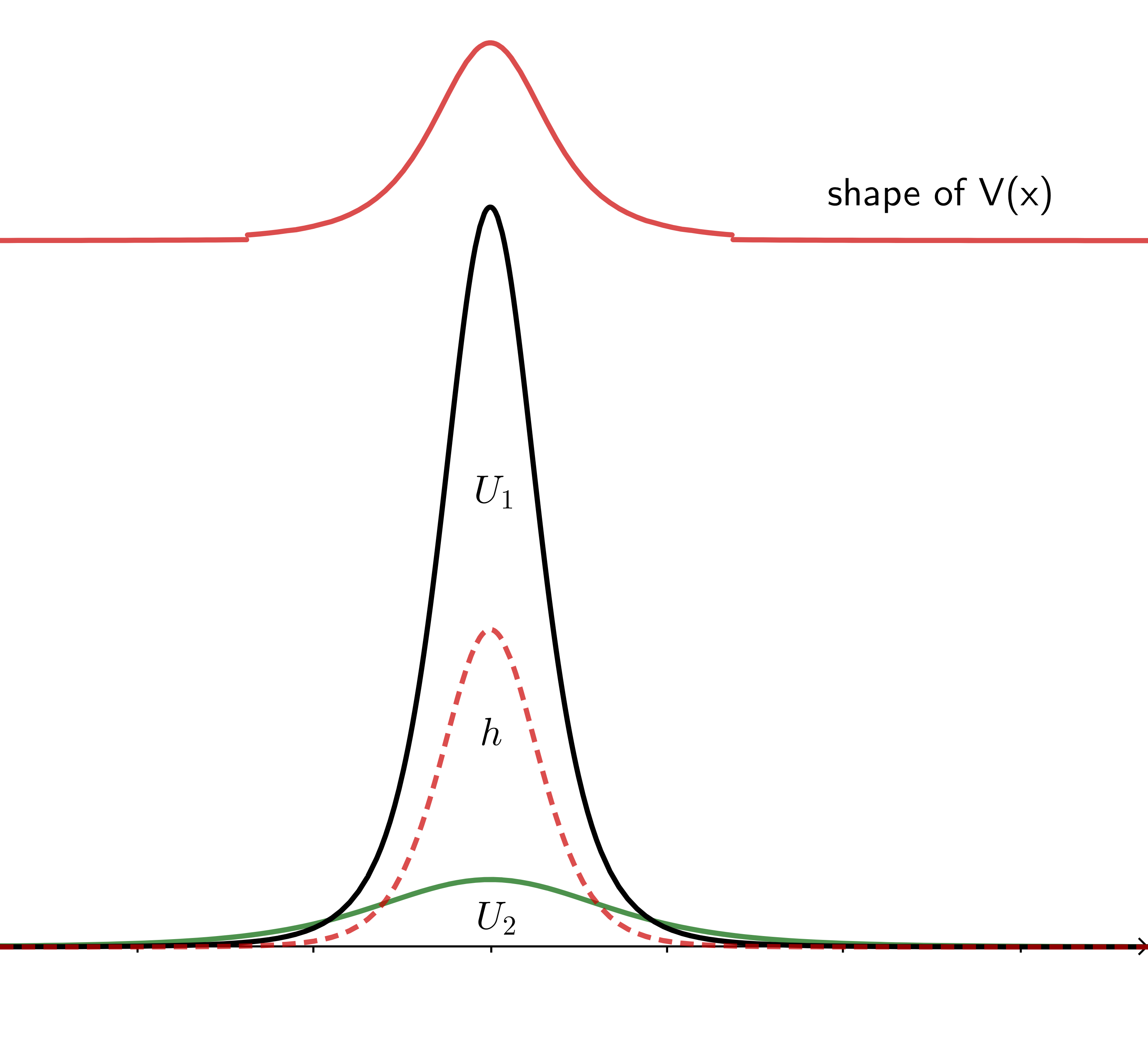
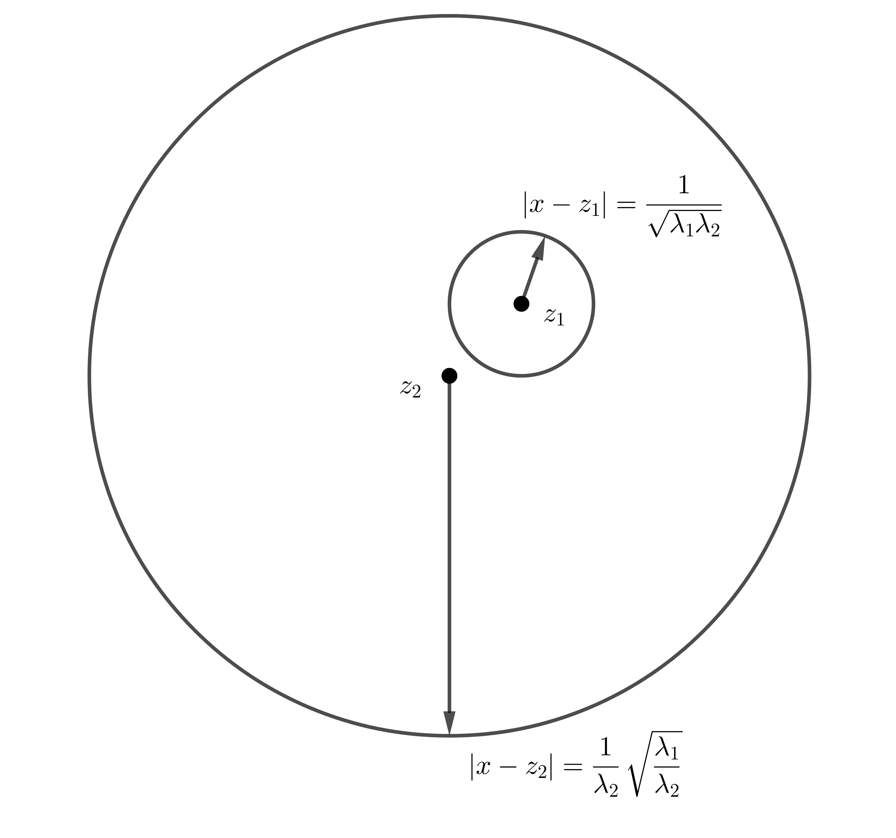
Figure 1. $U_{1}$ and $U_{2}$ form a bubble tower with $\lambda_{1}\gg\lambda_{2}$. The dotted line denotes the $h$. The right picture shows that the core region of $U_{2}$ (i.e. $\{|y_{2}|\leq R_{12}\}$) contains that of $U_{1}$ (i.e. $\{|y_{1}|\leq R_{12}\}$).

Bubble tower (see Figure 1): Without loss of generality (WLOG), we can assume $\lambda_{1}>\lambda_{2}$ and $R_{12}=\sqrt{\lambda_{1}/\lambda_{2}}=\varepsilon_{12}^{-1}\gg 1$. In the rescaled $z_{1}$-centered coordinate $y_{1}=\lambda_{1}(x-z_{1})$, we see that $U_{1}(x)=\lambda_{1}^{(n-2)/2}U(y_{1})$, where $U(y)=U[0,1](y)$, and

$$U_{2}(x)=\frac{\lambda_{1}^{(n-2)/2}R_{12}^{2-n}}{(1+\varepsilon_{12}^{4}|y_{1}-\xi_{2}|^{2})^{(n-2)/2}},$$ (3.9)

with $|\xi_{2}|=|\lambda_{1}(z_{2}-z_{1})|\leq R_{12}^{2}$. If $|y_{1}|\leq R_{12}/2$, then $U_{2}\lesssim U_{1}$,

$$h\lesssim U_{1}^{p-1}U_{2}\thickapprox\frac{\lambda_{1}^{(n+2)/2}R_{12}^{2-n}}{\langle y_{1}\rangle^{4}}.$$ (3.10)

If $R_{12}/3\leq|y_{1}|\leq 2R_{12}^{2}$, then $U_{1}\thickapprox\lambda_{1}^{(n-2)/2}|y_{1}|^{2-n}$ and $U_{2}\thickapprox\lambda_{1}^{(n-2)/2}R_{12}^{2-n}$. Setting $\hat{y}=y_{1}/R_{12}$, then

$$\begin{split}h\lesssim&\ \lambda_{1}^{(n+2)/2}R_{12}^{-(n+2)}\left|\left(1+\frac{1}{|\hat{y}|^{n-2}}\right)^{p}-1-\frac{1}{|\hat{y}|^{p(n-2)}}\right|\\ \lesssim&\ \frac{\lambda_{1}^{(n+2)/2}R_{12}^{-(n+2)}}{|\hat{y}|^{n-2}}\thickapprox\frac{\lambda_{1}^{(n+2)/2}R_{12}^{-4}}{\langle y_{1}\rangle^{n-2}}.\end{split}$$ (3.11)

On the other hand, in the rescaling $z_{2}$-centered coordinate $y_{2}=\lambda_{2}(x-z_{2})$, we see that $U_{2}(x)=\lambda_{2}^{(n-2)/2}U(y_{2})$ and

$$U_{1}(x)=\frac{\lambda_{2}^{(n-2)/2}R_{12}^{2-n}}{(\varepsilon_{12}^{4}+|y_{2}-\xi_{1}|^{2})^{(n-2)/2}},$$ (3.12)

where $\xi_{1}=\lambda_{2}(z_{1}-z_{2})$ with $|\xi_{1}|<1$. Keep in mind that $y_{2}-\xi_{1}=\varepsilon_{12}^{2}y_{1}$. Thus, if $1\leq|y_{2}-\xi_{1}|\leq R_{12}/2$, it means $R_{12}^{2}\leq|y_{1}|\leq R_{12}^{3}/2$. In this region, we have $U_{1}\lesssim U_{2}$,

$$h\lesssim U_{2}^{p-1}U_{1}\thickapprox\frac{\lambda_{2}^{(n+2)/2}R_{12}^{2-n}}{\langle y_{2}\rangle^{4}}.$$ (3.13)

In the outer region $|y_{2}-\xi_{2}|\geq R_{12}/3$, it is easy to see that

$$h\lesssim U_{2}^{p}\thickapprox\frac{\lambda_{1}^{(n+2)/2}R_{12}^{-2}}{\langle y_{1}\rangle^{n}}\lesssim\frac{\lambda_{1}^{(n+2)/2}R_{12}^{-4}}{\langle y_{1}\rangle^{n-2}}.$$ (3.14)

From (3.10), (3.11), (3.13) and (3.14), we conclude

$$\begin{split}h\lesssim&\ \sum_{i=1}^{2}\left(\frac{\lambda_{i}^{\frac{n+2}{2}}R_{12}^{2-n}}{\langle y_{i}\rangle^{4}}\chi_{\{|y_{i}|\leq R_{12}/2\}}+\frac{\lambda_{i}^{\frac{n+2}{2}}R_{12}^{-4}}{\langle y_{i}\rangle^{n-2}}\chi_{\{|y_{i}|\geq R_{12}/3\}}\right)\\ \leq&\ \sum_{i=1}^{2}\left(\frac{\lambda_{i}^{\frac{n+2}{2}}R^{2-n}}{\langle y_{i}\rangle^{4}}\chi_{\{|y_{i}|\leq R/2\}}+\frac{\lambda_{i}^{\frac{n+2}{2}}R^{-4}}{\langle y_{i}\rangle^{n-2}}\chi_{\{|y_{i}|\geq R/3\}}\right),\end{split}$$ (3.15)

for any $0<R\leq R_{12}$.

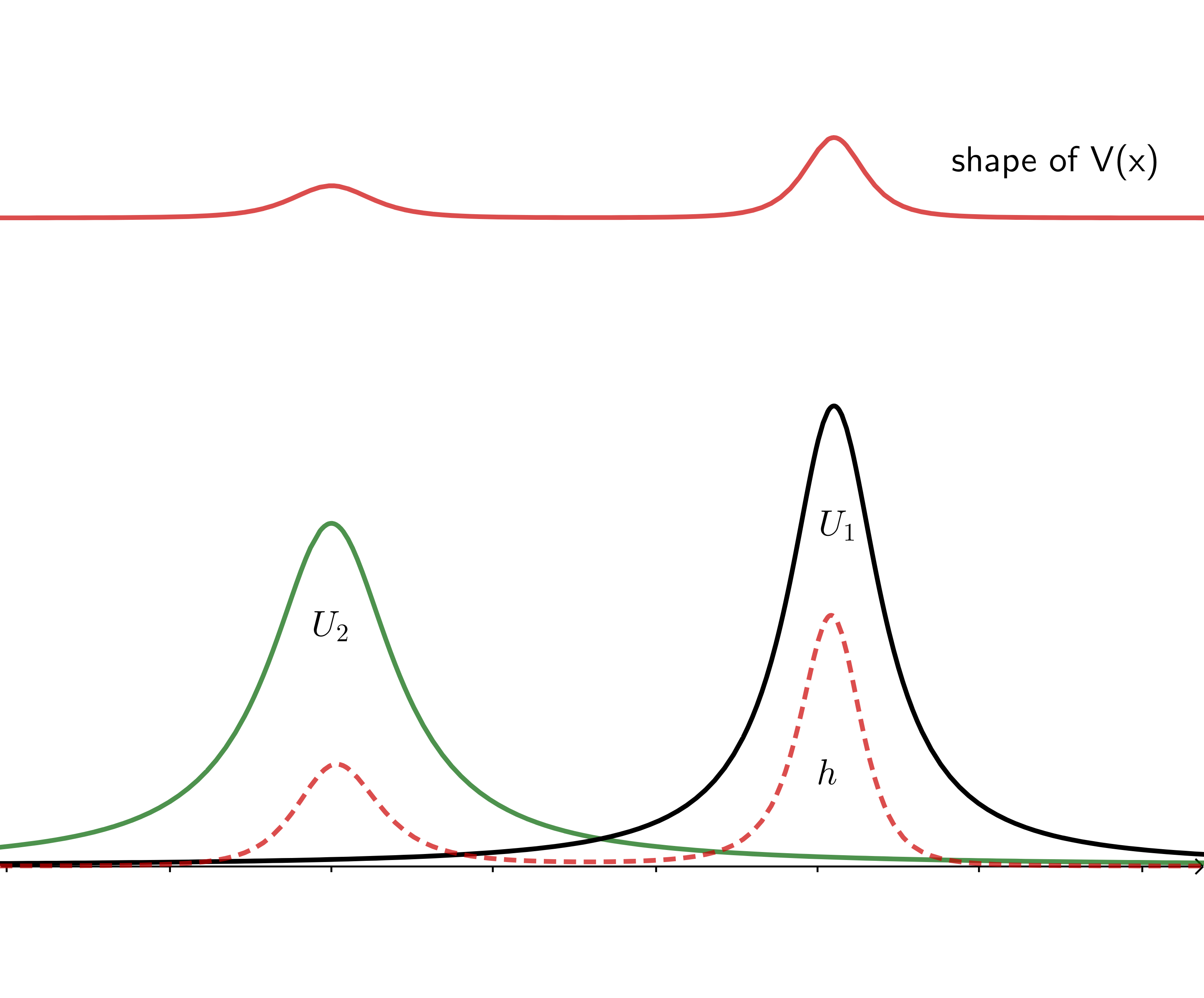
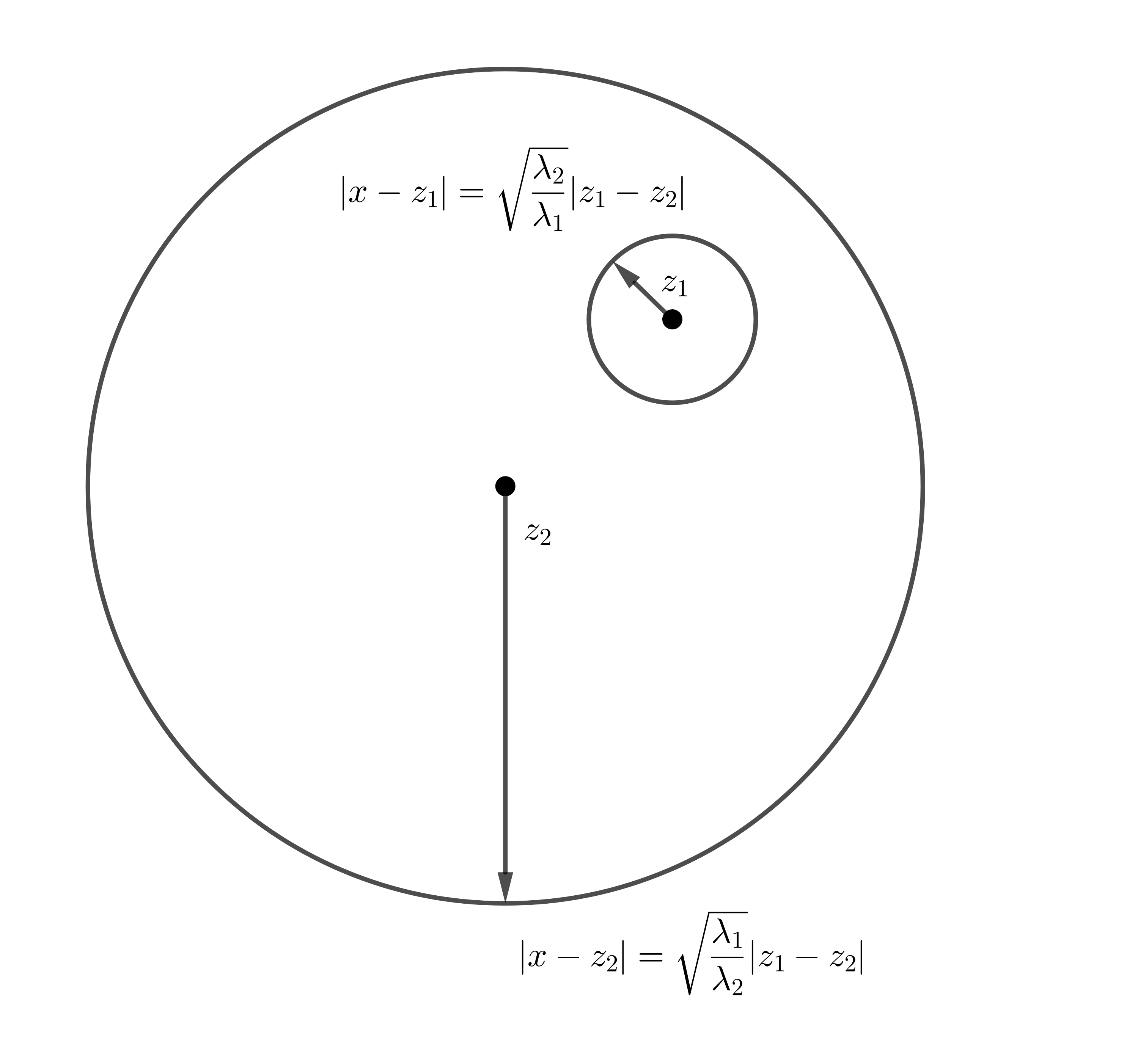
Figure 2. $U_{1}$ and $U_{2}$ form a bubble cluster. The right picture shows that the influence region of $U_{2}$ contains that of $U_{1}$ like bubble tower when $\lambda_{1}\gg\lambda_{2}$. However, if $\lambda_{1}\approx\lambda_{2}$, the core region of them shall be disjoint.

Bubble cluster (see Figure 2): WLOG, we can assume $\lambda_{1}\geq\lambda_{2}$ and $R_{12}=\sqrt{\lambda_{1}\lambda_{2}}|z_{1}-z_{2}|=\varepsilon_{12}^{-1}\gg 1$. In the rescaling $z_{1}$-centered coordinate $y_{1}=\lambda_{1}(x-z_{1})$, $U_{1}(x)=\lambda_{1}^{(n-2)/2}U(y_{1})$ and

$$U_{2}(x)=\frac{\lambda_{1}^{(n-2)/2}R_{12}^{2-n}}{(\frac{1}{\lambda_{2}^{2}|z_{1}-z_{2}|^{2}}+|\frac{y_{1}}{\lambda_{1}|z_{1}-z_{2}|}-e|^{2})^{(n-2)/2}},$$ (3.16)

with $e=(z_{2}-z_{1})/|z_{2}-z_{1}|$. Since $R_{12}\leq\lambda_{1}|z_{1}-z_{2}|$, if $|y_{1}|\leq R_{12}/2$, we have $U_{2}\lesssim U_{1}$,

$$h\lesssim U_{1}^{p-1}U_{2}\lesssim\frac{\lambda_{1}^{(n+2)/2}R_{12}^{2-n}}{\langle y_{1}\rangle^{4}}.$$ (3.17)

If $R_{12}/3\leq|y_{1}|\leq\lambda_{1}|z_{1}-z_{2}|/2$, then $U_{1}\thickapprox\lambda_{1}^{(n-2)/2}|y_{1}|^{2-n}$ and $U_{2}\thickapprox\lambda_{1}^{(n-2)/2}R_{12}^{2-n}$. Setting $\hat{y}=y_{1}/R_{12}$, then

$$\begin{split}h\lesssim&\ \lambda_{1}^{(n+2)/2}R_{12}^{-(n+2)}\left|\left(1+\frac{1}{|\hat{y}|^{n-2}}\right)^{p}-1-\frac{1}{|\hat{y}|^{p(n-2)}}\right|\\ \lesssim&\ \frac{\lambda_{1}^{(n+2)/2}R_{12}^{-(n+2)}}{|\hat{y}|^{n-2}}\thickapprox\frac{\lambda_{1}^{(n+2)/2}R_{12}^{-4}}{\langle y_{1}\rangle^{n-2}}.\end{split}$$ (3.18)

In the rescaling $z_{2}$-centered coordinate $y_{2}=\lambda_{2}(x-z_{2})$, $U_{2}(x)=\lambda_{2}^{(n-2)/2}U(y_{2})$ and

$$U_{1}(x)=\frac{\lambda_{2}^{(n-2)/2}R_{12}^{2-n}}{(\frac{1}{\lambda_{1}^{2}|z_{1}-z_{2}|^{2}}+|\frac{y_{2}}{\lambda_{2}|z_{1}-z_{2}|}+e|^{2})^{(n-2)/2}}.$$ (3.19)

If $|y_{2}|\leq R_{12}/2$ and $|y_{1}|\geq\lambda_{1}|z_{1}-z_{2}|/3$, it means $|\frac{y_{2}}{\lambda_{2}|z_{1}-z_{2}|}+e|\geq 1/3$, then

$$h\lesssim U_{2}^{p-1}U_{1}\lesssim\frac{\lambda_{2}^{(n+2)/2}R_{12}^{2-n}}{\langle y_{2}\rangle^{4}}.$$ (3.20)

In the outer region $|y_{2}|\geq R_{12}/3$ and $|y_{1}|\geq\lambda_{1}|z_{1}-z_{2}|/3\geq R_{12}/3$, we have

$$h\lesssim U_{1}^{p}+U_{2}^{p}\lesssim\frac{\lambda_{1}^{(n+2)/2}R_{12}^{-4}}{\langle y_{1}\rangle^{n-2}}+\frac{\lambda_{2}^{(n+2)/2}R_{12}^{-4}}{\langle y_{2}\rangle^{n-2}}.$$ (3.21)

From (3.17), (3.18), (3.20) and (3.21), we also have (3.15).

For any finite number of bubbles, we shall use a simple inequality (see Lemma A.6)

$$h=\sigma^{p}-\sum_{i=1}^{\nu}U_{i}^{p}\leq\sum_{i\neq j}[(U_{i}+U_{j})^{p}-U_{i}^{p}-U_{j}^{p}].$$

Each one on the RHS can be bounded by the above estimates of two bubbles, see (3.15). Summing them up, one can obtain $h\leq C(n,\nu)V(x)$. ∎

Remark 3.4.

In order to have a simple form of $V$, we bound $h$ just by $\langle y_{i}\rangle^{2-n}$ in (3.14) and (3.21). In fact, $h$ decays faster than $V$ at infinity. Such relaxation causes a minor problem for $n=6$ when estimating $\int_{|y_{i}|\geq R,|y_{j}|\geq R}VW$ in Proposition 3.9. Check the estimate (B.16) and (B.20) in Lemma B.2. Thanks to the fact that if $n=6$ then $p=2$ and $\sigma^{p}-\sum_{i=1}^{\nu}U_{i}^{p}=\sum_{i\neq j}U_{i}U_{j}$. We can get around this and directly estimate the integral $\int U_{i}U_{j}\rho_{0}$. Check the estimate (B.37) in Lemma B.3.

Lemma 3.5.

There exist a positive $\delta_{0}$ and a constant $C$, independent of $\delta$, such that for all $\delta\leqslant\delta_{0}$, if $\{U_{i}\}_{1\leq i\leq\nu}$ is a $\delta$-interacting bubble family and $\phi$ solves the equation

$$\begin{cases}\Delta\phi+p\sigma^{p-1}\phi=h,\\ \int U_{i}^{p-1}\phi Z_{i}^{a}=0,\quad i=1,\cdots,\nu;\ a=1,\cdots,n+1,\end{cases}$$ (3.22)

then

$$\|\phi\|_{*}\leq C\|h\|_{**}.$$ (3.23)

Proof.

We use blow-up arguments to prove (3.23). Suppose there are $k\to\infty$, $\frac{1}{k}$-interacting bubble families $\left\{U^{(k)}_{i}:=U[z^{(k)}_{i},\lambda^{(k)}_{i}]\right\}_{1\leq i\leq\nu}$, $h=h_{k}$ with $\|h_{k}\|_{**}\to 0$, and $\phi=\phi_{k}$ with $\|\phi_{k}\|_{*}=1$ solving the equation

$$\begin{cases}\Delta\phi_{k}+p\sigma_{k}^{p-1}\phi_{k}=h_{k},\quad&\text{in}\ \mathbb{R}^{n},\\ \int U_{i}^{p-1}Z_{i}^{a}\phi_{k}=0,\quad&i=1,\cdots,\nu;\,1\leq a\leq n+1.\end{cases}$$ (3.24)

For simplicity, here and after we denote $U_{i}:=U^{(k)}_{i}$ and $\sigma_{k}:=\sum_{i=1}^{\nu}U^{(k)}_{i}$.

In the beginning, let us introduce some notations. After finite steps of choosing subsequences, we can make the following assumptions. For each $i\in I=\{1,\cdots,\nu\}$, let $z^{(k)}_{ij}:=\lambda^{(k)}_{i}(z^{(k)}_{j}-z^{(k)}_{i})$, $j\in I\setminus\{i\}$, we can assume that $\lim_{k\to\infty}z^{(k)}_{ij}$ exists or $\lim_{k\to\infty}z^{(k)}_{ij}=\infty$. Then we divide indices $I\setminus\{i\}$ into two groups:

$$\begin{split}I_{i,1}&:=\{j\in I\setminus\{i\}\ |\ \lim_{k\to\infty}z^{(k)}_{ij}\ \text{exists and}\ \lim_{k\to\infty}|z^{(k)}_{ij}|<\infty\},\\ I_{i,2}&:=\{j\in I\setminus\{i\}\ |\ \lim_{k\to\infty}z^{(k)}_{ij}=\infty\}.\end{split}$$ (3.25)

Furthermore, we divide all bubbles into four groups: ones are higher (lower) than $U_{i}$ in tower relationship, ones are much higher (otherwise) than $U_{i}$ in cluster relationship.

$$\begin{split}T^{+}_{i}&:=\{j\in I\setminus\{i\}\ |\ \lambda^{(k)}_{j}\geq\lambda^{(k)}_{j},R^{(k)}_{ij}=\sqrt{\lambda^{(k)}_{j}/\lambda^{(k)}_{i}}\},\\ T^{-}_{i}&:=\{j\in I\setminus\{i\}\ |\ \lambda^{(k)}_{j}<\lambda^{(k)}_{i},R^{(k)}_{ij}=\sqrt{\lambda^{(k)}_{i}/\lambda^{(k)}_{j}}\},\\ C^{+}_{i}&:=\{j\in I\setminus\{i\}\ |\ \lim_{k\to\infty}\lambda^{(k)}_{j}/\lambda^{(k)}_{i}=\infty,R^{(k)}_{ij}=\sqrt{\lambda^{(k)}_{i}\lambda^{(k)}_{j}}|z^{(k)}_{i}-z^{(k)}_{j}|\},\\ C^{-}_{i}&:=\{j\in I\setminus\{i\}\ |\ \lim_{k\to\infty}\lambda^{(k)}_{j}/\lambda^{(k)}_{i}<\infty,R^{(k)}_{ij}=\sqrt{\lambda^{(k)}_{i}\lambda^{(k)}_{j}}|z^{(k)}_{i}-z^{(k)}_{j}|\}.\end{split}$$ (3.26)

Recall that $y^{(k)}_{i}=\lambda^{(k)}_{i}(x-z^{(k)}_{i})$. Let us define

$$\begin{split}\Omega^{(k)}&:=\bigcup_{i\in I}\{|y^{(k)}_{i}|\leq L\},\\ \Omega^{(k)}_{i}&:=\{|y^{(k)}_{i}|\leq L\}\bigcap\left(\bigcap_{j\in I,j\neq i}\{|y^{(k)}_{i}-z^{(k)}_{ij}|\geq\epsilon\}\right),\end{split}$$ (3.27)

with a large constant $L=L(n,\nu)$ and a small constant $\epsilon=\epsilon(n,\nu)$ to be determined later (see Figure 3 for an illustration of $\Omega_{1}$). It is easy to see that, for large $k$, we have

$$\begin{split}\Omega^{(k)}_{i}&:=\{|y^{(k)}_{i}|\leq L\}\bigcap\left(\bigcap_{j\in T^{+}_{i}\cup C^{+}_{i}}\{|y^{(k)}_{i}-z^{(k)}_{ij}|\geq\epsilon\}\right).\end{split}$$ (3.28)

For simplicity, here and after we drop the superscript if there is no confusion. It is convenient to denote $W=\sum_{i\in I}(w_{i,1}+w_{i,2})$ and $V=\sum_{i\in I}(v_{i,1}+v_{i,2})$ with

$$\begin{split}w_{i,1}(x)=\frac{\lambda_{i}^{\frac{n-2}{2}}R^{2-n}}{\langle y_{i}\rangle^{2}}\chi_{\{|y_{i}|\leq R\}},\quad w_{i,2}(x)=\frac{\lambda_{i}^{\frac{n-2}{2}}R^{-4}}{\langle y_{i}\rangle^{n-4}}\chi_{\{|y_{i}|\geq R/2\}},\\ v_{i,1}(x)=\frac{\lambda_{i}^{\frac{n+2}{2}}R^{2-n}}{\langle y_{i}\rangle^{4}}\chi_{\{|y_{i}|\leq R\}},\quad v_{i,2}(x)=\frac{\lambda_{i}^{\frac{n+2}{2}}R^{-4}}{\langle y_{i}\rangle^{n-2}}\chi_{\{|y_{i}|\geq R/2\}},\end{split}$$ (3.29)

where $R=R^{(k)}=\frac{1}{2}\min_{i\neq j}\{R^{(k)}_{ij}\}\to\infty$ as $k\to\infty$.

Since $\|\phi_{k}\|_{*}=1$, we have $|\phi_{k}|(x)\leq W(x)$ and there exists a sequence of points $\{x_{k}\}_{k\in\mathbb{N}}$ such that

$$|\phi_{k}|(x_{k})=W(x_{k}).$$ (3.30)

First, going to a subsequence if necessary, we consider the case that $\{x_{k}\}_{k\in\mathbb{N}}\subset\Omega$.

Case 1: $\{x_{k}\}_{k\in\mathbb{N}}\subset\Omega_{i_{0}}$ for some $i_{0}\in I$. Let $i_{0}=1$ and define

$$\begin{cases}\tilde{\phi}_{k}(y_{1}):=W^{-1}(x_{k})\phi_{k}(x)\quad\text{with}\ y_{1}=\lambda_{1}(x-z_{1}),\\ \tilde{h}_{k}(y_{1}):=\lambda_{1}^{-2}W^{-1}(x_{k})h_{k}(x),\quad\tilde{\sigma}_{k}(y_{1}):=\sigma_{k}(x).\end{cases}$$ (3.31)

Then $\tilde{\phi}_{k}$ satisfy

$$\begin{cases}\Delta\tilde{\phi}_{k}(y_{1})+p\lambda_{1}^{-2}\tilde{\sigma}_{k}^{p-1}(y_{1})\tilde{\phi}_{k}(y_{1})=\tilde{h}_{k}(y_{1})\quad&\text{in}\ \mathbb{R}^{n},\\ \int U^{p-1}Z^{a}\tilde{\phi}_{k}dy_{1}=0,\quad&1\leq a\leq n+1.\end{cases}$$ (3.32)

Here $U=U[0,1](y_{1})$ and $Z^{a}=Z^{a}(y_{1})=Z_{1}^{a}(x)$ defined in (3.1). Let $\tilde{z}_{j}=z^{(k)}_{1j}$ , $\bar{z}_{j}=\lim_{k\to\infty}\tilde{z}^{(k)}_{1j}$ and

$$E_{1}:=\bigcap_{j\in T^{+}_{1}\cap I_{1,1}}\{|y_{1}-\bar{z}_{j}|\geq 1/M\},\quad E_{2}:=\bigcap_{j\in C^{+}_{1}\cap I_{1,1}}\{|y_{1}-\bar{z}_{j}|\geq|\bar{z}_{j}|/M\}.$$

Let

$$\begin{split}K_{M}:=&\ \{|y_{1}|\leq M\}\cap E_{1}\cap E_{2}.\end{split}$$ (3.33)

Suppose $M\geq 2\max\{L,\epsilon^{-1}\}$, it is easy to see that $\Omega^{(k)}_{i}\subset\subset K_{M}$ for $k$ large.

Claim 1.

In each compact subset $K_{M}$, it holds that, as $k\to\infty$,

$$\begin{split}\lambda_{1}^{-2}\tilde{\sigma}_{k}^{p-1}\to\ U[0,1],\quad|\tilde{h}_{k}|\to\ 0,\end{split}$$ (3.34)

uniformly. Moreover, we have

$$|\tilde{\phi}_{k}|(y_{1})\lesssim|y_{1}-\tilde{z}_{j}|^{4-n},\quad j\in T^{+}_{1}\cup C^{+}_{1}.$$ (3.35)

We postpone the proof of Claim 1 and finish the blow-up argument in Case 1. By the standard elliptic regularity theorem, the Claim 1 shows that there exists a subsequence of $\tilde{\phi}_{k}$ uniformly converges in each $K_{M}$. Furthermore, by the diagonal arguments, let $M\to\infty$, we have a subsequence of $\tilde{\phi}_{k}$ weakly converges to $\tilde{\phi}$ with

$$\begin{cases}\Delta\tilde{\phi}+pU^{p-1}\tilde{\phi}=0,\quad&\text{in}\ \mathbb{R}^{n}\setminus\{\bar{z}_{j}\ |\ j\in(T^{+}_{1}\cup C^{+}_{1})\cap I_{1,1}\},\\ |\tilde{\phi}|(y_{1})\lesssim|y_{1}-\bar{z}_{j}|^{4-n},\quad&j\in(T^{+}_{1}\cup C^{+}_{1})\cap I_{1,1},\\ \int U^{p-1}Z^{a}\tilde{\phi}dy_{1}=0,\quad&1\leq a\leq n+1.\end{cases}$$ (3.36)

Notice that all singular $\bar{z}_{j}$ are removable. Together with the non-degeneracy of Talenti bubbles, we get $\tilde{\phi}\equiv 0$. However, since $|Y_{k}|\leq L$, going to a subsequence if necessary, then $\lim_{k\to\infty}Y_{k}=Y_{\infty}$ and consequently $\tilde{\phi}(Y_{\infty})=1$. This is a contradiction.

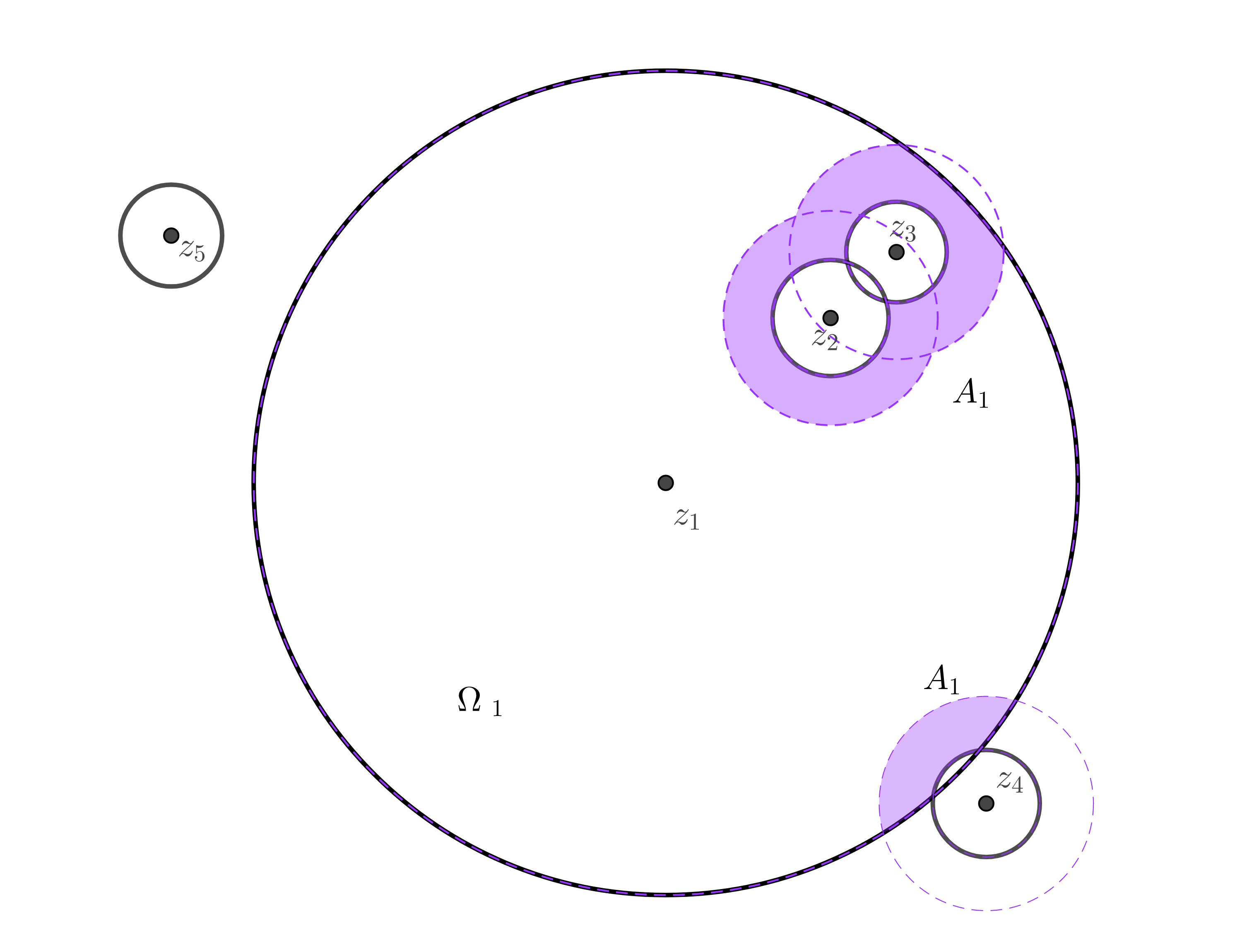
Figure 3. Illustration for the blow-up regions of a simple bubble configuration. The solid circles denote $\{y_{i}=L\}$ for $i=1,\cdots,5$. The dashed circles mean $\{|y_{1}-\tilde{z}_{1j}|=\epsilon\}$. The shaded regions constitute $A_{1}$.

Case 2: $\{x_{k}\}_{k\in\mathbb{N}}\subset\Omega\setminus\left(\cup_{i\in I}\Omega_{i}\right)$. There exist some $i\in I$ such that, choosing a subsequence if necessary, $\{x_{k}\}_{k\in\mathbb{N}}\subset A_{i}$ where

$$A_{i}:=\bigcup_{j\in J_{i}}\left\{|y_{i}|\leq L,\ |y_{i}-\tilde{z}_{ij}|\leq\epsilon,\ |y_{j}|\geq L\right\},\quad J_{i}=T^{+}_{i}\cup C^{+}_{i}.$$ (3.37)

We can choose the smallest $A_{i_{0}}$ such that, for each $A_{i}\supset\{x_{k}\}_{k\in\mathbb{N}}$, it holds that $\lambda_{i_{0}}\geq\lambda_{i}$. For simplicity, let $i_{0}=1$ and take notations as before. See Figure 3 for $A_{i}$ in a simple case. Define

$$\begin{split}\tilde{W}(x):=&\ \sum_{j\in J_{1}}(w_{j,1}(x)+w_{j,2}(x))+w_{1,1}(x),\\ \tilde{V}(x):=&\ \sum_{j\in J_{1}}(v_{j,1}(x)+v_{j,2}(x))+v_{1,1}(x).\end{split}$$ (3.38)

We will use the following two claims to show that $\tilde{W}(x)$ is a supersolution to our problem in the region $A_{1}$.

Claim 2.

For any two bubbles, say $U_{i}$ and $U_{j}$, suppose $k$ large enough, in the region $\{|y_{i}|\geq L,|y_{j}|\geq L\}$ it holds that

$$\sum_{m,l\in\{i,j\}}U_{m}^{p-1}(w_{l,1}+w_{l,2})\leq\epsilon_{1}\sum_{l\in\{i,j\}}(v_{l,1}+v_{l,2}),$$ (3.39)

with small $\epsilon_{1}=\max\{L^{\frac{-4}{n-2}},2^{n}L^{-\frac{1}{2}},2\epsilon^{2}\}$.

Claim 3.

Fix a bubble $U_{i}$, let $J_{i}=T^{+}_{i}\cup C^{+}_{i}$. In the region $A_{i}$, we have

$$U_{i}^{p-1}\sum_{j\in J_{i}}(w_{j,1}+w_{j,2})\leq \ \epsilon_{1}\sum_{j\in J_{i}}(v_{j,1}+v_{j,2}),$$ (3.40)

$$\sum_{j\in J_{i}}U_{j}^{p-1}w_{i,1}\leq \ \epsilon_{1}\sum_{j\in J_{i}}(v_{j,1}+v_{j,2})+\epsilon_{1}v_{i,1},$$ (3.41)

when $k$ large enough.

We also postpone the proofs of Claim 2 and Claim 3. By (3.29), it is easy to see $\Delta\tilde{W}\leq-2(n-4)\tilde{V}$. In the region $A_{1}$, it is easy to see $\sum_{j\in T^{-}_{1}\cup C^{-}_{1}}U_{j}\ll U_{1}$ for $k$ large. Therefore

$$\sigma_{k}^{p-1}=\left(\sum_{j\in J_{1}}U_{j}+U_{1}+\sum_{j\in T^{-}_{1}\cup C^{-}_{1}}U_{j}\right)^{p-1}\leq\sum_{j\in J_{1}}U_{j}^{p-1}+\frac{5}{4}U_{1}^{p-1}.$$

Consequently, it follows from Claim 2 and Claim 3 that

$$\begin{split}\sigma_{k}^{p-1}\tilde{W}=&\ \sum_{i,j\in J_{1}}U_{i}^{p-1}\left(w_{j,1}+w_{j,2}\right)+\frac{5}{4}U_{1}^{p-1}\sum_{j\in J_{1}}\left(w_{j,1}+w_{j,2}\right)\\ &\ +w_{1,1}\sum_{j\in J_{1}}U_{j}^{p-1}+\frac{5}{4}U_{1}^{p-1}w_{1,1}\\ \leq&\ (4\nu^{2}\epsilon_{1}+\frac{5}{4})\tilde{V}\quad\text{in}\ A_{1}.\end{split}$$ (3.42)

Then, by choosing $L$ large and $\epsilon$ small such that $(4\nu^{2}\epsilon_{1}+5/4)p\leq 3$,

$$\Delta\tilde{W}+p\sigma_{k}^{p-1}\tilde{W}\leq-\tilde{V}\quad\text{in}\ A_{1}.$$ (3.43)

From Case 1, we conclude that, for $k$ large,

$$|\phi_{k}|(x)\leq C\|h_{k}\|_{**}W(x)\quad\text{in}\ \cup_{i\in I}\Omega_{i},$$ (3.44)

with a constant $C=C(n,\nu)$. On the other hand, if $i\in T^{-}_{1}$, then $|y_{i}|=\frac{\lambda_{i}}{\lambda_{1}}|y_{1}-\tilde{z}_{i}|\leq L$. We have, for $k$ large,

$$\begin{split}\frac{w_{1,1}}{w_{i,1}}=&\ \left(\frac{\lambda_{1}}{\lambda_{i}}\right)^{\frac{n-2}{2}}\frac{\langle y_{i}\rangle^{2}}{\langle y_{1}\rangle^{2}}\geq L^{-2}\left(\frac{\lambda_{1}}{\lambda_{i}}\right)^{\frac{n-2}{2}}\gg 1,\\ \frac{v_{1,1}}{v_{i,1}}=&\ \left(\frac{\lambda_{1}}{\lambda_{i}}\right)^{\frac{n+2}{2}}\frac{\langle y_{i}\rangle^{4}}{\langle y_{1}\rangle^{4}}\geq L^{-4}\left(\frac{\lambda_{1}}{\lambda_{i}}\right)^{\frac{n+2}{2}}\gg 1.\end{split}$$ (3.45)

If $i\in C^{-}_{1}$, then $|y_{i}|=\frac{\lambda_{i}}{\lambda_{1}}|y_{1}-\tilde{z}_{i}|\geq\frac{\lambda_{i}|\tilde{z}_{i}|}{2\lambda_{1}}=\frac{\lambda_{i}|z_{1}-z_{i}|}{2}$. We have

$$\begin{split}\frac{w_{1,1}}{w_{i,2}}=&\ R^{6-n}\left(\frac{\lambda_{1}}{\lambda_{i}}\right)^{\frac{n-2}{2}}\frac{\langle y_{i}\rangle^{n-4}}{\langle y_{1}\rangle^{2}}\geq 2^{4-n}L^{-2}R^{2}\left(\frac{\lambda_{1}}{\lambda_{i}}\right)\gg 1,\\ \frac{v_{1,1}}{v_{i,2}}=&\ R^{6-n}\left(\frac{\lambda_{1}}{\lambda_{i}}\right)^{\frac{n+2}{2}}\frac{\langle y_{i}\rangle^{n-2}}{\langle y_{1}\rangle^{4}}\geq 2^{2-n}L^{-4}R^{4}\left(\frac{\lambda_{1}}{\lambda_{i}}\right)^{2}\gg 1.\end{split}$$ (3.46)

From (3.44), (3.45), and (3.46), we have

$$\begin{split}W=&\ \tilde{W}+\sum_{j\in T^{-}_{1}\cup C^{-}_{1}}(w_{j,1}+w_{j,2})\leq 2\tilde{W}\quad\text{in}\ A_{1},\\ V=&\ \tilde{V}+\sum_{j\in T^{-}_{1}\cup C^{-}_{1}}(v_{j,1}+v_{j,2})\leq 2\tilde{V}\quad\text{in}\ A_{1}.\end{split}$$ (3.47)

By (3.42), (3.44) and (3.47), it is easy to see that $\pm 10C\|h_{k}\|_{**}\tilde{W}$ is an upper (lower) barrier for $\phi_{k}$ in $A_{1}$. It follows that

$$|\phi_{k}|(x_{k})\tilde{W}^{-1}(x_{k})\leq 10C\|h_{k}\|_{**}\to 0.$$ (3.48)

It contradicts to (3.30) since $W(x_{k})\geq\tilde{W}(x_{k})$.

Case 3: $\{x_{k}\}_{k\in\mathbb{N}}\subset\Omega^{c}=\cup_{i\in I}\{|y_{i}|\geq L\}$. As before, it is easy to see that $\Delta W\leq-2(n-4)V$. From Claim 2, we also have

$$\begin{split}\sigma_{k}^{p-1}W\leq&\ \nu^{2}\epsilon_{1}V\quad\text{in}\ \Omega^{c}.\end{split}$$ (3.49)

Then,

$$\Delta W+p\sigma_{k}^{p-1}W\leq-V\quad\text{in}\ \Omega^{c}.$$ (3.50)

From Case 1 and Case 2, we conclude that, for $k$ large,

$$|\phi_{k}|(x)\leq C\|h_{k}\|_{**}W(x)\quad\text{in}\ \Omega.$$ (3.51)

In particular, we have

$$|\phi_{k}|(x)\leq C\|h_{k}\|_{**}W(x)\quad\text{on}\ \partial\Omega^{c}=\partial\Omega.$$ (3.52)

Thus $\pm C\|h_{k}\|_{**}W$ is an upper (lower) barrier for $\phi_{k}$ in $\Omega^{c}$. It follows that

$$|\phi_{k}|(x_{k})W^{-1}(x_{k})\leq C\|h_{k}\|_{**}\to 0.$$ (3.53)

It contradicts to (3.30).

To complete the proof of (3.23), it suffices to prove the three claims above.

Proof of Claim 1.

To prove the claim, we need to use a simple inequality

$$\frac{\sum_{i}a_{i}}{\sum_{i}b_{i}}\leq\max_{i}\{\frac{a_{i}}{b_{i}}\},$$ (3.54)

holds for any positive numbers $a_{i},b_{i}$. Thus by (3.32)

$$|\tilde{\phi}_{k}|(y_{1})=\frac{|\phi_{k}(x)|}{W(x_{k})}\leq\frac{W(x)}{W_{k}(x)}\leq\max_{j}\left\{\frac{w_{j,1}(x)+w_{j,2}(x)}{w_{j,1}(x_{k})+w_{j,2}(x_{k})}\right\},$$

$$|\tilde{h}_{k}|(x)=\frac{|h_{k}(x)|}{\lambda_{1}^{2}W(x_{k})}\leq\|h_{k}\|_{**}\frac{V(x)}{\lambda_{1}^{2}W(x_{k})}\leq\|h_{k}\|_{**}\max_{j}\left\{\frac{v_{j,1}(x)+v_{j,2}(x)}{\lambda_{1}^{2}w_{j,1}(x_{k})+\lambda_{1}^{2}w_{j,2}(x_{k})}\right\}.$$

We shall estimate the RHS of the above two equations on each compact subset $K_{M}$. They are divided into the following four cases.

The case $j\in T^{+}_{1}$. By (3.12), we have

$$U_{j}(x)\thickapprox\frac{\lambda_{j}^{\frac{n-2}{2}}}{\langle y_{j}\rangle^{n-2}}\thickapprox\frac{\lambda_{1}^{\frac{n-2}{2}}R_{1j}^{2-n}}{(\varepsilon_{1j}^{2}+|y_{1}-\tilde{z}_{j}|)^{n-2}}\lesssim M^{n-2}\lambda_{1}^{\frac{n-2}{2}}R_{1j}^{2-n}.$$ (3.55)

Let $Y_{k}=\lambda_{1}(x_{k}-z_{1})$. Since $|y_{j}|=R_{1j}^{2}|y_{1}-\tilde{z}_{j}|\geq R_{1j}^{2}/M\geq R$ for $k$ large, we only need to consider

$$\frac{w_{j,2}(x)}{w_{j,2}(x_{k})}\thickapprox \ \frac{(\varepsilon_{1j}^{2}+|Y_{k}-\tilde{z}_{j}|)^{n-4}}{(\varepsilon_{1j}^{2}+|y_{1}-\tilde{z}_{j}|)^{n-4}}\lesssim\frac{1}{|y_{1}-\tilde{z}_{j}|^{n-4}},$$ (3.56)

$$\frac{v_{j,2}(x)}{\lambda_{1}^{2}w_{j,2}(x_{k})}\thickapprox \ \frac{(\varepsilon_{1j}^{2}+|Y_{k}-\tilde{z}_{j}|)^{n-4}}{(\varepsilon_{1j}^{2}+|y_{1}-\tilde{z}_{j}|)^{n-2}}\lesssim M^{n-2}.$$ (3.57)

The case $j\in T^{-}_{1}$. By (3.9), we have

$$U_{j}(x)\thickapprox\frac{\lambda_{1}^{\frac{n-2}{2}}R_{1j}^{2-n}}{(1+\varepsilon_{1j}^{2}|y_{1}-\tilde{z}_{j}|)^{n-2}}\lesssim\lambda_{1}^{\frac{n-2}{2}}R_{1j}^{2-n}.$$ (3.58)

It holds that $|y_{j}|=R_{1j}^{-2}|y_{1}-\tilde{z}_{j}|\leq MR_{1j}^{-2}\leq R$ for $k$ large. Then we have

$$\frac{w_{j,1}(x)}{w_{j,1}(x_{k})}\thickapprox \ \frac{(1+\varepsilon_{1j}^{2}|Y_{k}-\tilde{z}_{j}|)^{2}}{(1+\varepsilon_{1j}^{2}|y_{1}-\tilde{z}_{j}|)^{2}}\lesssim 1,$$ (3.59)

$$\frac{v_{j,1}(x)}{\lambda_{1}^{2}w_{j,1}(x_{k})}\thickapprox \ R_{1j}^{-4}\frac{(1+\varepsilon_{1j}^{2}|Y_{k}-\tilde{z}_{j}|)^{2}}{(1+\varepsilon_{1j}^{2}|y_{1}-\tilde{z}_{j}|)^{4}}\lesssim R_{1j}^{-4}.$$ (3.60)

The case $j\in C^{+}_{1}$. Let $\lambda=\lambda_{j}/\lambda_{1}$, then $R_{1j}=\sqrt{\lambda}|\tilde{z}_{j}|$ and $|\tilde{z}_{j}|\geq 1$. It holds that, no matter $|\bar{z}_{j}|<\infty$ or $|\bar{z}_{j}|=\infty$, we have $|y_{j}|=\lambda|y_{1}-\tilde{z}_{j}|\geq\sqrt{\lambda}R_{1j}/M\geq R$ for $k$ large. Then

$$U_{j}(x)\thickapprox\frac{\lambda_{1}^{\frac{n-2}{2}}}{(\lambda^{-1/2}+\lambda^{1/2}|y_{1}-\tilde{z}_{j}|)^{n-2}}\lesssim\lambda_{1}^{\frac{n-2}{2}}M^{n-2}R_{1j}^{2-n}.$$ (3.61)

Then we have

$$\frac{w_{j,2}(x)}{w_{j,2}(x_{k})}\thickapprox \ \frac{(\lambda^{-1/2}+\lambda^{1/2}|Y_{k}-\tilde{z}_{j}|^{2})^{n-4}}{(\lambda^{-1/2}+\lambda^{1/2}|y_{1}-\tilde{z}_{j}|)^{n-4}}\lesssim\frac{1}{|y_{1}-\tilde{z}_{j}|^{n-4}},$$ (3.62)

$$\frac{v_{j,2}(x)}{\lambda_{1}^{2}w_{j,2}(x_{k})}\thickapprox \ \lambda R_{1j}^{-2}\frac{(\lambda^{-1/2}+\lambda^{1/2}|Y_{k}-\tilde{z}_{j}|)^{n-4}}{(\lambda^{-1/2}+\lambda^{1/2}|y_{1}-\tilde{z}_{j}|)^{n-2}}$$

$$\lesssim \ M^{n-2}R_{1j}^{-2}|\tilde{z}_{j}|^{-2}\leq M^{n-2}R_{1j}^{-2}.$$ (3.63)

The case $j\in C^{-}_{1}$. Let $\lambda=\lambda_{j}/\lambda_{1}$, then $R_{1j}=\sqrt{\lambda}|\tilde{z}_{j}|\leq(1+\theta_{j})|\tilde{z}_{j}|$ with $\theta_{j}=\lim_{k\to\infty}\lambda^{(k)}_{j}/\lambda^{(k)}_{1}$. It holds that $|y_{1}|\leq M\leq|\tilde{z}_{j}|/2$ for $k$ large. Then $|y_{1}-\tilde{z}_{j}|\geq|\tilde{z}_{j}|/2$,

$$U_{j}(x)\thickapprox\frac{\lambda_{1}^{\frac{n-2}{2}}}{(\lambda^{-1/2}+\lambda^{1/2}|y_{1}-\tilde{z}_{j}|)^{n-2}}\lesssim\lambda_{1}^{\frac{n-2}{2}}R_{1j}^{2-n}.$$ (3.64)

Furthermore, we have

$$\frac{w_{j,2}(x)}{w_{j,2}(x_{k})}\thickapprox \ \frac{(\lambda^{-1/2}+\lambda^{1/2}|Y_{k}-\tilde{z}_{j}|^{2})^{n-4}}{(\lambda^{-1/2}+\lambda^{1/2}|y_{1}-\tilde{z}_{j}|)^{n-4}}\lesssim R_{1j}^{4-n},$$ (3.65)

$$\frac{v_{j,2}(x)}{\lambda_{1}^{2}w_{j,2}(x_{k})}\thickapprox \ \lambda R_{1j}^{-2}\frac{(\lambda^{-1/2}+\lambda^{1/2}|Y_{k}-\tilde{z}_{j}|)^{n-4}}{(\lambda^{-1/2}+\lambda^{1/2}|y_{1}-\tilde{z}_{j}|)^{n-2}}\lesssim R_{1j}^{-n}.$$ (3.66)

It is easy to see that

$$U_{1}(x)=U(y_{1}),\quad\frac{w_{1,1}(x)}{w_{1,1}(x_{k})}\thickapprox \ \frac{\langle Y_{k}\rangle^{2}}{\langle y_{1}\rangle^{2}}\lesssim 1,\quad\frac{v_{1,1}(x)}{\lambda_{1}^{2}w_{1,1}(x_{k})}\thickapprox\frac{\langle Y_{k}\rangle^{2}}{\langle y_{1}\rangle^{4}}\lesssim 1.$$ (3.67)

From (3.55), (3.58), (3.61), (3.64) and (3.67), we get

$$\lambda_{1}^{-2}\tilde{\sigma}_{k}^{p-1}(y_{1})=U[0,1](y_{1})+o(1)\to U[0,1](y_{1}).$$ (3.68)

From (3.55), (3.58), (3.61), (3.64) and (3.67), we get

$$\begin{split}|\tilde{h}_{k}|\leq&\ \|h_{k}\|_{**}\frac{V(x)}{\lambda_{1}^{2}W(x_{k})}\lesssim M^{n-2}\|h_{k}\|_{**}\to 0.\end{split}$$ (3.69)

From (3.56), (3.59), (3.62), (3.65) and (3.67), we see that the singularities only happen for $j\in(T^{+}_{1}\cup C^{+}_{1})\cap I_{1,1}$ with

$$|\tilde{\phi}_{k}|(y_{1})\lesssim|y_{1}-\tilde{z}_{j}|^{4-n}.$$ (3.70)

∎

Proof of the Claim 2.

Here and after, we always assume $k$ is large enough. WLOG, we assume $i=1$ and $j=2$. It is easy to see the claim holds when $m=l$,

$$\sum_{l=1}^{2}U_{i}^{p-1}(w_{l,1}+w_{l,2})\leq\epsilon_{1}\sum_{l=1}^{2}(v_{l,1}+v_{l,2}).$$ (3.71)

It reduces to consider the case $m\neq l$. We divide it to the following two main cases.

(1) The case $\lambda_{1}\geq\lambda_{2}$ and $R_{12}=\sqrt{\lambda_{1}/\lambda_{2}}$. Let $\xi_{1}=\lambda_{2}(z_{1}-z_{2})$ and $\xi_{2}=\lambda_{1}(z_{2}-z_{1})$. It holds that $|\xi_{1}|\leq 1$ and $|\xi_{2}|\leq R_{12}^{2}$. Since $y_{1}=R_{12}^{2}(y_{2}-\xi_{1})$, then $\langle y_{1}\rangle\geq\frac{1}{2}R_{12}^{2}\langle y_{2}\rangle$ on the set $\{|y_{1}|\geq L,|y_{2}|\geq L\}$. We have

$$\begin{split}U_{1}^{p-1}(w_{2,1}+w_{2,2})=&\ \frac{\lambda_{1}^{2}}{\langle y_{1}\rangle^{4}}(w_{2,1}+w_{2,2})\leq\ 16\lambda_{2}^{2}\langle y_{2}\rangle^{-4}(w_{2,1}+w_{2,2})\\ \leq&\ 16\langle y_{2}\rangle^{-2}(v_{2,1}+v_{2,2})\leq\epsilon_{1}(v_{2,1}+v_{2,2}).\end{split}$$ (3.72)

Observe that $|y_{1}-\xi_{2}|=R_{12}^{2}|y_{2}|\geq LR_{12}^{2}$, then $|y_{1}|\geq(L-1)R_{12}^{2}$. In the region $\{|y_{1}|\geq L,|y_{2}|\geq L\}$, we get

$$\begin{split}U_{2}^{p-1}(w_{1,1}+w_{1,2})=&\ \frac{\lambda_{2}^{2}}{\langle y_{2}\rangle^{4}}\frac{\lambda_{1}^{\frac{n-2}{2}}R^{-4}}{\langle y_{1}\rangle^{n-4}}\chi_{\{|y_{1}|\geq(L-1)R_{12}^{2}\}}.\end{split}$$ (3.73)

First, we bound the above term on the set $\{L\leq|y_{2}|\leq LR_{12},|y_{1}|\geq(L-1)R_{12}^{2}\}$, that is

$$\begin{split}\frac{\lambda_{2}^{2}}{\langle y_{2}\rangle^{4}}\frac{\lambda_{1}^{\frac{n-2}{2}}R^{-4}}{\langle y_{1}\rangle^{n-4}}=&\ \frac{\lambda_{2}^{\frac{n+2}{2}}R^{-4}}{\langle y_{2}\rangle^{4}}\frac{R_{12}^{n-2}}{\langle y_{1}\rangle^{n-4}}\leq\ (L-1)^{4-n}\frac{\lambda_{2}^{\frac{n+2}{2}}R^{-4}}{\langle y_{2}\rangle^{4}}\frac{1}{R_{12}^{n-6}}\\ \leq&\ \frac{L^{n-6}}{(L-1)^{n-4}}\left(\frac{\lambda_{2}^{\frac{n+2}{2}}R^{2-n}}{\langle y_{2}\rangle^{4}}\chi_{\{|y_{2}|\leq R\}}+\frac{\lambda_{2}^{\frac{n+2}{2}}R^{-4}}{\langle y_{2}\rangle^{n-2}}\chi_{\{R\leq|y_{2}|\leq LR_{12}\}}\right)\\ \leq&\ \epsilon_{1}(v_{2,1}+v_{2,2}).\end{split}$$ (3.74)

Second, on $\{|y_{2}|\geq LR_{12},|y_{1}|\geq(L-1)R_{12}^{2}\}$, we have $\langle y_{1}\rangle=\langle R_{12}^{2}(y_{2}-\xi_{1})\rangle\geq\frac{1}{2}R_{12}^{2}\langle y_{2}\rangle$,

$$\begin{split}\frac{\lambda_{2}^{2}}{\langle y_{2}\rangle^{4}}\frac{\lambda_{1}^{\frac{n-2}{2}}R^{-4}}{\langle y_{1}\rangle^{n-4}}=&\ \frac{\lambda_{2}^{\frac{n+2}{2}}R^{-4}}{\langle y_{2}\rangle^{4}}\frac{R_{12}^{n-2}}{\langle y_{1}\rangle^{n-4}}\leq\ v_{2,2}\frac{\langle y_{2}\rangle^{n-6}R_{12}^{n-2}}{\langle y_{1}\rangle^{n-4}}\leq\epsilon_{1}v_{2,2}.\end{split}$$ (3.75)

(2) The case $\lambda_{1}\geq\lambda_{2}$ and $R_{12}=\sqrt{\lambda_{1}\lambda_{2}}|z_{1}-z_{2}|$. Notice that $|\xi_{2}|=\sqrt{\lambda_{1}/\lambda_{2}}R_{12}$ and $y_{2}=\lambda_{2}\lambda_{1}^{-1}(y_{1}-\xi_{2})$. Then on the set $\{L\leq|y_{1}|\leq\frac{1}{2}\sqrt{\lambda_{1}/\lambda_{2}}R_{12}\}$, we have $\langle y_{2}\rangle\geq\frac{1}{2}\sqrt{\lambda_{2}/\lambda_{1}}R_{12}$. Consequently

$$U_{2}^{p-1}w_{1,1}=\frac{\lambda_{2}^{2}}{\langle y_{2}\rangle^{4}}\frac{\lambda_{1}^{\frac{n-2}{2}}R^{2-n}}{\langle y_{1}\rangle^{2}}\chi_{\{L\leq|y_{1}|\leq R\}}\leq 16\lambda_{1}^{2}R_{12}^{-4}\frac{\lambda_{1}^{\frac{n-2}{2}}R^{2-n}}{\langle y_{1}\rangle^{2}}\leq\epsilon_{1}v_{1,1}.$$ (3.76)

Next consider $U_{2}^{p-1}w_{1,2}$. To bound it, we divide it into two cases. First, suppose $\lambda_{2}|z_{1}-z_{2}|\geq{L}^{\frac{1}{4}}$, then on the set $\{R<|y_{1}|<\frac{1}{2}\sqrt{\lambda_{1}/\lambda_{2}}R_{12}\}$

$$U_{2}^{p-1}w_{1,2}\leq 16\lambda_{1}^{2}R_{12}^{-4}\frac{\lambda_{1}^{\frac{n-2}{2}}R^{-4}}{\langle y_{1}\rangle^{n-4}}=16v_{1,2}\frac{\langle y_{1}\rangle^{2}}{R_{12}^{4}}<\frac{16}{\lambda_{2}^{2}|z_{1}-z_{2}|^{2}}v_{1,2}\leq\frac{16}{\sqrt{L}}v_{1,2}.$$ (3.77)

On the set $\{|y_{1}|>\frac{1}{2}\sqrt{\lambda_{1}/\lambda_{2}}R_{12}\}$, then

$$U_{2}^{p-1}w_{1,2}=\frac{\lambda_{2}^{2}}{\langle y_{2}\rangle^{4}}\frac{\lambda_{1}^{\frac{n-2}{2}}R^{-4}}{\langle y_{1}\rangle^{n-4}}=v_{2,1}\frac{(\lambda_{1}/\lambda_{2})^{\frac{n-2}{2}}R^{n-6}}{\langle y_{1}\rangle^{n-4}}<\frac{2^{n-4}}{\lambda_{2}^{2}|z_{1}-z_{2}|^{2}}v_{2,1}<\frac{2^{n-4}}{\sqrt{L}}v_{2,1}.$$

Second, suppose $|\xi_{1}|=\lambda_{2}|z_{1}-z_{2}|\leq L^{\frac{1}{4}}$. On the set $\{L\leq|y_{2}|\leq R\}$, since $y_{1}=\lambda_{1}\lambda_{2}^{-1}(y_{2}-\xi_{1})$, then $|y_{1}|\geq\frac{\lambda_{1}}{\lambda_{2}}\frac{L}{2}\geq\frac{\sqrt{L}}{2}R_{12}^{2}$ and

$$U_{2}^{p-1}w_{1,2}=\frac{\lambda_{2}^{2}}{\langle y_{2}\rangle^{4}}\frac{\lambda_{1}^{\frac{n-2}{2}}R^{-4}}{\langle y_{1}\rangle^{n-4}}\leq v_{2,1}\frac{(\lambda_{1}/\lambda_{2})^{\frac{n-2}{2}}R^{n-6}}{(\frac{1}{2}\sqrt{L}R_{12}^{2})^{n-4}}\leq(\frac{1}{2}\sqrt{L})^{4-n}v_{2,1}\leq\epsilon_{1}v_{2,1}.$$

On the set $\{|y_{2}|\geq R\}$,

$$U_{2}^{p-1}w_{1,2}=v_{2,2}\frac{(\frac{\lambda_{1}}{\lambda_{2}})^{\frac{n-2}{2}}\langle y_{2}\rangle^{n-6}}{\langle y_{1}\rangle^{n-4}}\leq v_{2,2}\frac{(\frac{\lambda_{1}}{\lambda_{2}})^{\frac{n-2}{2}}\langle y_{2}\rangle^{n-6}}{\langle\frac{1}{2}\frac{\lambda_{1}}{\lambda_{2}}y_{2}\rangle^{n-4}}\leq v_{2,2}\frac{2^{n-4}(\frac{\lambda_{1}}{\lambda_{2}})^{\frac{6-n}{2}}}{\langle y_{2}\rangle^{2}}\leq\epsilon_{1}v_{2,2}.$$

Let us consider the term $U_{1}^{p-1}w_{2,1}$. On the set $\{L<|y_{2}|<R,|y_{1}|<R\}$, one has $\langle y_{2}\rangle\geq\frac{1}{2}\sqrt{\lambda_{2}/\lambda_{1}}R_{12}$ and

$$U_{1}^{p-1}w_{2,1}=\frac{\lambda_{1}^{2}}{\langle y_{1}\rangle^{4}}\frac{\lambda_{2}^{\frac{n-2}{2}}R^{2-n}}{\langle y_{2}\rangle^{2}}\leq\frac{\lambda_{1}^{2}}{\langle y_{1}\rangle^{4}}\frac{\lambda_{2}^{\frac{n-2}{2}}R^{2-n}}{(\frac{1}{2}\sqrt{\lambda_{2}/\lambda_{1}}R_{12})^{2}}=4(\frac{\lambda_{2}}{\lambda_{1}})^{\frac{n-4}{2}}R_{12}^{-2}v_{1,1}\leq\epsilon v_{1,1}.$$

On the set $\{L<|y_{2}|<R,R<|y_{1}|\}\cap\{L(\lambda_{2}/\lambda_{1})^{2}v_{1,2}\geq v_{2,1}\}$, one has

$$U_{1}^{p-1}w_{2,1}=\frac{\lambda_{1}^{2}}{\langle y_{1}\rangle^{4}}\frac{\lambda_{2}^{\frac{n-2}{2}}R^{2-n}}{\langle y_{2}\rangle^{2}}=v_{2,1}\frac{\langle y_{2}\rangle^{2}}{\langle y_{1}\rangle^{4}}(\frac{\lambda_{1}}{\lambda_{2}})^{2}\leq\frac{L\langle y_{2}\rangle^{2}}{\langle y_{1}\rangle^{4}}v_{1,2}\leq LR^{-2}v_{1,2}.$$ (3.78)

On the set $\{L<|y_{2}|<R,R<|y_{1}|\}\cap\{L(\lambda_{2}/\lambda_{1})^{2}v_{1,2}\leq v_{2,1}\}$, one has $\langle y_{1}\rangle^{n-2}\geq L(\lambda_{1}/\lambda_{2})^{\frac{n-2}{2}}R^{n-6}\langle y_{2}\rangle^{4}$, then

$$U_{1}^{p-1}w_{2,1}=v_{2,1}\frac{\langle y_{2}\rangle^{2}}{\langle y_{1}\rangle^{4}}\left(\frac{\lambda_{1}}{\lambda_{2}}\right)^{2}\leq v_{2,1}L^{-\frac{4}{n-2}}R^{-\frac{4(n-6)}{n-2}}\langle y_{2}\rangle^{\frac{2n-20}{n-2}}\leq\epsilon_{1}v_{2,1}$$ (3.79)

here we have use $L\leq|y_{2}|\leq R$.

It remains to consider the term $U_{1}^{p-1}w_{2,2}$. First, on the set $\{|y_{2}|\geq R,|y_{1}|\leq R\}$, similar to (3.76), one has

$$U_{1}^{p-1}w_{2,2}=\frac{\lambda_{1}^{2}}{\langle y_{1}\rangle^{4}}\frac{\lambda_{2}^{\frac{n-2}{2}}R^{-4}}{\langle y_{2}\rangle^{n-4}}\leq\frac{\lambda_{1}^{2}}{\langle y_{1}\rangle^{4}}\frac{\lambda_{2}^{\frac{n-2}{2}}R^{2-n}}{\langle y_{2}\rangle^{2}}\leq\epsilon_{1}v_{1,1}$$ (3.80)

Second, on the set $\{|y_{2}|\geq R,|y_{1}|\geq R\}\cap\{v_{1,2}\geq v_{2,2}\}$, one has $\langle y_{1}\rangle/\langle y_{2}\rangle\leq(\frac{\lambda_{1}}{\lambda_{2}})^{\frac{n+2}{2(n-2)}}$,

$$U_{1}^{p-1}w_{2,2}=\frac{\lambda_{1}^{2}}{\langle y_{1}\rangle^{4}}\frac{\lambda_{2}^{\frac{n-2}{2}}R^{-4}}{\langle y_{2}\rangle^{n-4}}\leq v_{1,2}\frac{\langle y_{1}\rangle^{n-6}}{\langle y_{2}\rangle^{n-4}}\left(\frac{\lambda_{2}}{\lambda_{1}}\right)^{\frac{n-2}{2}}\leq v_{1,2}\frac{1}{\langle y_{2}\rangle^{2}}\left(\frac{\lambda_{2}}{\lambda_{1}}\right)^{\frac{8}{n-2}}\leq\epsilon_{1}v_{1,2}.$$

On the set $\{|y_{2}|\geq R,|y_{1}|\geq R\}\cap\{v_{1,2}\leq v_{2,2}\}$, one has $\langle y_{1}\rangle\geq\langle y_{2}\rangle(\lambda_{1}/\lambda_{2})^{\frac{n+2}{2(n-2)}}$

$$U_{1}^{p-1}w_{2,2}=\frac{\lambda_{1}^{2}}{\langle y_{1}\rangle^{4}}\frac{\lambda_{2}^{\frac{n-2}{2}}R^{-4}}{\langle y_{2}\rangle^{n-4}}=v_{2,2}\left(\frac{\lambda_{1}}{\lambda_{2}}\right)^{2}\frac{\langle y_{2}\rangle^{2}}{\langle y_{1}\rangle^{4}}\leq v_{2,2}\frac{(\lambda_{2}/\lambda_{1})^{\frac{8}{n-2}}}{\langle y_{2}\rangle^{2}}\leq\epsilon_{1}v_{2,2}.$$

∎

Proof of the Claim 3.

WLOG we assume $i=1$. By the definition (3.26), we have $\lambda_{j}\gg\lambda_{1}$. Let $\lambda=\lambda_{j}/\lambda_{1}$, $\xi_{1}=\lambda_{j}(z_{1}-z_{j})$ and $\xi_{j}=\tilde{z}_{j}=\lambda_{1}(z_{j}-z_{1})$. Observe that, if $j\in C^{+}_{1}$, $|y_{j}|\leq R\ll\sqrt{\lambda}R_{1j}=|\xi_{1}|$, then $|y_{j}-\xi_{1}|\geq|\xi_{1}|/2$. Thus, on the set $\{L\leq|y_{j}|\leq R\}$, no matter $j\in C_{1}^{+}$ or $T_{1}^{+}$,

$$\lambda\langle y_{1}\rangle^{2}=\lambda+\lambda^{-1}|y_{j}-\xi_{1}|^{2}\geq\frac{1}{2}R_{1j}^{2},\quad j\in T^{+}_{1}\cup C^{+}_{1}.$$ (3.81)

It follows from (3.81) that, on the set $\{L\leq|y_{j}|\leq R\}$,

$$\begin{split}U_{1}^{p-1}w_{j,1}=&\ \frac{\lambda_{1}^{2}}{\langle y_{1}\rangle^{4}}\frac{\lambda_{j}^{\frac{n-2}{2}}R^{2-n}}{\langle y_{j}\rangle^{2}}\leq\ 16R_{1j}^{-4}\frac{\lambda_{j}^{\frac{n+2}{2}}R^{2-n}}{\langle y_{j}\rangle^{2}}\leq\epsilon_{1}v_{j,1}.\end{split}$$ (3.82)

Moreover, on the set $\{|y_{j}|\geq R,|y_{1}-\xi_{j}|\leq\epsilon\}$, it holds that $\langle y_{j}\rangle^{2}=1+\lambda^{2}|y_{1}-\xi_{j}|^{2}\leq 2\lambda^{2}\epsilon^{2}$ and

$$\begin{split}U_{1}^{p-1}w_{j,2}=\ \frac{\lambda_{1}^{2}}{\langle y_{1}\rangle^{4}}\frac{\lambda_{j}^{\frac{n-2}{2}}R^{-4}}{\langle y_{j}\rangle^{n-4}}=\frac{\langle y_{j}\rangle^{2}}{\lambda^{2}\langle y_{1}\rangle^{4}}v_{j,2}\leq 2\epsilon^{2}v_{j,2}\leq\epsilon_{1}v_{j,2}.\end{split}$$ (3.83)

Together with (3.82) and (3.83), we prove the (3.40).

If $L\leq|y_{j}|\leq R$, it is easy to see that

$$\begin{split}U_{j}^{p-1}w_{1,1}=\frac{\lambda_{j}^{2}}{\langle y_{j}\rangle^{4}}\frac{\lambda_{1}^{\frac{n-2}{2}}R^{2-n}}{\langle y_{1}\rangle^{2}}=\ \frac{\lambda^{\frac{2-n}{2}}}{\langle y_{1}\rangle^{2}}v_{j,1}\leq\epsilon_{1}v_{j,1}.\end{split}$$ (3.84)

For $|y_{j}|>R$, one can use the same type of estimates (3.78) and (3.79) to prove

$$U_{j}^{p-1}w_{1,1}\leq\epsilon_{1}(v_{j,2}+v_{1,1}).$$

∎

Combining the above claims, we complete the proof. ∎

Next, we estimate the coefficients $c_{b}^{j}$ in (3.2).

Lemma 3.6.

Suppose $\sigma$ is the sum of a family of $\delta$-interacting bubbles. If $\phi$, $h$ and $c_{b}^{j}$ satisfy (3.2), then

$$|c_{b}^{j}|\lesssim Q\|h\|_{**}+Q^{p}\|\phi\|_{*},\quad 1\leq j\leq\nu,\ 1\leq b\leq n+1.$$

Proof.

We shall multiply (3.2) by $Z_{j}^{b}$. By the Lemma A.5, for $a,b\leq n+1$, there exist some constants $\gamma^{b}$ such that

$$\sum_{i,a}\int c_{a}^{i}U_{i}^{p-1}Z_{i}^{a}Z_{j}^{b}=c_{b}^{j}\gamma^{b}+\sum_{i\neq j}\sum_{a=1}^{n+1}c_{a}^{i}O(q_{ij}).$$

Fix $1\leq j\leq\nu$, $1\leq b\leq n+1$. By the orthogonal condition in (3.2) and $|Z_{j}^{b}|\lesssim U_{j}$

$$\begin{split}\left|\int p\sigma^{p-1}\phi Z_{j}^{b}\right|=&\ \left|\int p\left(\sigma^{p-1}-U_{j}^{p-1}\right)Z_{j}^{b}\phi\right|\\ \lesssim&\ \|\phi\|_{*}\int\left(\sigma^{p-1}-U_{j}^{p-1}\right)U_{j}Wdx.\end{split}$$ (3.85)

Now we use the fact that, $(\sigma^{p-1}-U_{i}^{p-1})U_{i}\geq 0$ for each $i$,

$$(\sigma^{p-1}-U_{j}^{p-1})U_{j}\leq\sum_{i}(\sigma^{p-1}-U_{i}^{p-1})U_{i}=\sigma^{p}-\sum_{i}U_{i}^{p}.$$

Then by Proposition (3.3),(3.85) can be bounded by

$$\begin{split}\left|\int p\sigma^{p-1}\phi Z_{j}^{b}\right|\lesssim&\ \|\phi\|_{*}\int(\sigma^{p}-\sum_{i=1}^{\nu}U_{i}^{p})Wdx\lesssim\|\phi\|_{*}\int V(x)W(x)dx\lesssim\ Q^{p}\|\phi\|_{*}.\end{split}$$

Here we have used Lemma B.2 in the last inequality (see similar estimates (3.107)) and (3.109)). Similarly, by Lemma B.4 we have

$$\begin{split}\left|\int hZ_{j}^{b}\right|\lesssim&\ \|h\|_{**}\sum_{i=1}^{\nu}\int VU_{j}dx\lesssim\ Q\|h\|_{**}.\end{split}$$ (3.86)

Multiplying (3.2) by $Z_{j}^{b}$ and integrating, we see that $\{c_{b}^{j}\}$ satisfy the linear system

$$c_{b}^{j}\gamma^{b}+\sum\limits_{i\neq j}\sum\limits_{a=1}^{n+1}c_{a}^{i}O(q_{ij})=\int p\sigma^{p-1}\phi Z_{j}^{b}+\int hZ_{j}^{b},\quad 1\leq j\leq\nu,\ 1\leq b\leq n+1.$$

Since $q_{ij}\leq Q\leq\delta$ the system is solvable and we prove the claim. ∎

From Lemma 3.5 and 3.6, using the same argument as in the proof of Proposition 4.1 in [11], we can prove the following result:

Proposition 3.7.

There exists positive $\delta_{0}$ and a constant $C>0$, independent of $\delta$, such that for all $\delta\leqslant\delta_{0}$ and all $h$ with $\|h\|_{**}<\infty$, problem (3.2) has a unique solution $\phi\equiv L_{\delta}(h).$ Besides,

$$\left\|L_{\delta}(h)\right\|_{*}\leqslant C\|h\|_{**},\quad\left|c_{a}^{i}\right|\leqslant C\delta\|h\|_{**}.$$

Proposition 3.8.

Suppose that $\delta$ is small enough. There exists a solution $\rho_{0}$ and a family of scalars $(c_{a}^{i})$ which solve

$$\Delta\phi+[(\sigma+\phi)^{p}-\sigma^{p}]+\sigma^{p}-\sum_{i=1}^{\nu}U_{i}^{p}=\sum_{i,a}c_{a}^{i}U_{i}^{p}Z_{i}^{a}$$ (3.87)

with

$$|\rho_{0}|(x)\leq CW(x).$$ (3.88)

Proof.

Let

$$N_{1}(\phi)= (\sigma+\phi)^{p}-\sigma^{p}-p\sigma^{p-1}\phi,$$ (3.89)

$$N_{2}= \sigma^{p}-\sum_{i=1}^{\nu}U_{i}^{p}.$$ (3.90)

Then, (3.87) is equivalent to

$$\phi=A(\phi)=:-L_{\delta}(N_{1}(\phi))-L_{\delta}(N_{2}),$$ (3.91)

where $L_{\delta}$ is defined in Proposition 3.7. We will show that $A$ is a contraction mapping.

First, it follows from Proposition 3.3 that there exists $C_{2}=C_{2}(n,\nu)$

$$\|N_{2}\|_{**}\leq C_{2}.$$ (3.92)

Next, we claim that $\|N_{1}(\phi)\|_{**}\leq C_{1}R^{-4(p-1)}\|\phi\|_{*}$. In fact, since $|N_{1}(\phi)|\leq C|\phi|^{p}\leq C\|\phi\|_{*}^{p}W^{p}$, then

$$\begin{split}\|N_{1}(\phi)\|_{**}\leq C\|\phi\|_{*}\sup_{\mathbb{R}^{n}}W^{p}(x)V^{-1}(x).\end{split}$$ (3.93)

Notice, for the first type weight function, say $|y_{i}|\leq R$, we have

$$\left(\frac{\lambda_{i}^{\frac{n-2}{2}}R^{2-n}}{\langle y_{i}\rangle^{2}}\right)^{p}\left(\frac{\langle y_{i}\rangle^{4}}{\lambda_{i}^{\frac{n+2}{2}}R^{2-n}}\right)=R^{-4}\langle y_{i}\rangle^{4-2p}\leq R^{-4}.$$ (3.94)

For the second type weight, say $R/2\leq|y_{i}|$, we have

$$\begin{split}\left(\frac{\lambda_{i}^{\frac{n-2}{2}}R^{-4}}{\langle y_{i}\rangle^{n-4}}\right)^{p}\left(\frac{\langle y_{i}\rangle^{n-2}}{\lambda_{i}^{\frac{n+2}{2}}R^{-4}}\right)=R^{-4(p-1)}\langle y_{i}\rangle^{n-2-p(n-4)}\leq R^{-4(p-1)},\end{split}$$ (3.95)

since $n-2-p(n-4)\leq 0$. By the inequality (3.54), we get

$$W^{p}V^{-1}\leq R^{-4(p-1)}.$$ (3.96)

Thus, there exists $C_{1}=C_{1}(n,\nu)$ such that

$$\begin{split}\|N_{1}(\phi)\|_{**}\leq C_{1}R^{-4(p-1)}\|\phi\|_{*}.\end{split}$$ (3.97)

Making $C_{1}$ possibly larger so that we also have $\|L_{\delta}(h)\|_{*}\leq C_{1}\|h\|_{**}$ in Proposition 3.7.

Now define the space

$$E=\{u:\ u\in C(\mathbb{R}^{n})\cap D^{1,2}(\mathbb{R}^{n}),\|u\|_{*}\leq C_{1}C_{2}+1\}.$$ (3.98)

We claim that $A$ is a contraction mapping from $E$ to $E$. In fact, choosing $\delta$ small, then $R$ large such that $R^{-4(p-1)}C_{1}^{2}(C_{1}C_{2}+1)\leq 1$, we have

$$\begin{split}\|A(\phi)\|_{*}\leq&\ C_{1}\|N_{1}(\phi)\|_{**}+C_{1}\|N_{2}\|_{**}\\ \leq&\ R^{-4(p-1)}C^{2}_{1}(C_{1}C_{2}+1)+C_{1}C_{2}\leq C_{1}C_{2}+1.\end{split}$$ (3.99)

Thus, $A(E)\subset E$. Furthermore,

$$\begin{split}\|A(\phi_{1})-A(\phi_{2})\|_{*}\leq&\ \|L_{\delta}(N_{1}(\phi_{1}))-L_{\delta}(N_{1}(\phi_{2}))\|_{**}\\ \leq&\ C_{1}\|N_{1}(\phi_{1})-N_{1}(\phi_{2})\|_{**}.\end{split}$$ (3.100)

If $n\geq 6$, then $N_{1}^{\prime}(t)\leq C|t|^{p-1}$. As a result,

$$\begin{split}|N_{1}(\phi_{1})-N_{1}(\phi_{2})|\leq&\ C\left(|\phi_{1}|^{p-1}+|\phi_{2}|^{p-1}\right)|\phi_{1}-\phi_{2}|\\ \leq&\ C\left(\|\phi_{1}\|_{*}^{p-1}+\|\phi_{2}\|_{*}^{p-1}\right)\|\phi_{1}-\phi_{2}\|_{*}W^{p}.\end{split}$$ (3.101)

Since $W^{p}V^{-1}\leq R^{-4(p-1)}\ll 1$ if $\delta$ small, we get

$$\|A(\phi_{1})-A(\phi_{2})\|_{*}\leq\frac{1}{2}\|\phi_{1}-\phi_{2}\|_{*}.$$ (3.102)

Thus, $A$ is a contraction. It follows from the contraction mapping theorem that there is a unique $\phi\in E$, such that $\phi=A(\phi)$. Moreover, it follows Proposition 3.7 that $\|\phi\|_{*}\leq C$. ∎

3.2. Some estimates of the error

In this subsection, we will establish $L^{2}$ estimates for the $\nabla\rho$, based on the point-wise estimates from the previous subsection.

Proposition 3.9.

Suppose $\delta$ is small enough. We have the gradient estimates

$$\|\nabla\rho_{0}\|_{L^{2}}\lesssim\begin{cases}Q|\log Q|^{\frac{1}{2}},&\text{if }n=6,\\ Q^{\frac{p}{2}},&\text{if }n\geq 7.\end{cases}$$ (3.103)

Proof.

Multiplying $\rho_{0}$ to (3.87) to get

$$\int|\nabla\rho_{0}|^{2}\lesssim\int\sigma^{p-1}\rho_{0}^{2}+\int|\rho_{0}|^{p+1}+\int(\sigma^{p}-\sum U_{i}^{p})\rho_{0}.$$ (3.104)

It follows from Proposition 3.8 that $|\rho_{0}(x)|\lesssim W(x)$. By the Lemma B.1, we have

$$\begin{split}\int\sigma^{p-1}\rho_{0}^{2}&\lesssim\ \sum_{i=1}^{\nu}\int U_{i}^{p-1}\rho_{0}^{2}\\ \lesssim&\ \sum_{i=1}^{\nu}\left(\int_{|y_{i}|\leq R}\frac{\lambda_{i}^{2}}{\langle y_{i}\rangle^{4}}\frac{\lambda_{i}^{n-2}R^{4-2n}}{\langle y_{i}\rangle^{4}}dx+\int_{|y_{i}|\geq R/2}\frac{\lambda_{i}^{2}}{\langle y_{i}\rangle^{4}}\frac{\lambda_{i}^{n-2}R^{-8}}{\langle y_{i}\rangle^{2n-8}}dx\right)\\ &\ +\sum_{i\neq j}\left(\int_{|y_{i}|\leq R}\frac{\lambda_{j}^{2}}{\langle y_{j}\rangle^{4}}\frac{\lambda_{i}^{n-2}R^{4-2n}}{\langle y_{i}\rangle^{4}}dx+\int_{|y_{i}|\geq R/2}\frac{\lambda_{j}^{2}}{\langle y_{j}\rangle^{4}}\frac{\lambda_{i}^{n-2}R^{-8}}{\langle y_{i}\rangle^{2n-8}}dx\right)\\ \lesssim&\ R^{-n-2}\thickapprox Q^{p}.\end{split}$$ (3.105)

By Sobolev inequality, we have

$$\int|\rho_{0}|^{p+1}\lesssim\|\nabla\rho_{0}\|_{L^{2}}^{p+1}.$$ (3.106)

Now consider the last term in (3.104). Proposition 3.3 says that $|\sigma^{p}-\sum_{i}U_{i}^{p}|\lesssim V(x)$.

$\bullet$ If $n\geq 7$, using (3.6) and (3.7), we obtain

$$\begin{split}&\left|\int(\sigma^{p}-\sum U_{i}^{p})\rho_{0}\right|\lesssim\int V(x)W(x)\\ &\leq\sum_{i,j=1}^{\nu}\int_{\begin{subarray}{c}|y_{i}|\leq R\\ |y_{j}|\leq R\end{subarray}}\frac{\lambda_{i}^{\frac{n+2}{2}}R^{2-n}}{\langle y_{i}\rangle^{4}}\frac{\lambda_{j}^{\frac{n-2}{2}}R^{2-n}}{\langle y_{j}\rangle^{2}}+\int_{\begin{subarray}{c}|y_{i}|\leq R\\ |y_{j}|\geq R/2\end{subarray}}\frac{\lambda_{i}^{\frac{n+2}{2}}R^{2-n}}{\langle y_{i}\rangle^{4}}\frac{\lambda_{j}^{\frac{n-2}{2}}R^{-4}}{\langle y_{j}\rangle^{n-4}}\\ &+\sum_{i,j=1}^{\nu}\int_{\begin{subarray}{c}|y_{i}|\geq R/2\\ |y_{j}|\leq R\end{subarray}}\frac{\lambda_{i}^{\frac{n+2}{2}}R^{-4}}{\langle y_{i}\rangle^{n-2}}\frac{\lambda_{j}^{\frac{n-2}{2}}R^{2-n}}{\langle y_{j}\rangle^{2}}+\int_{\begin{subarray}{c}|y_{i}|\geq R/2\\ |y_{j}|\geq R/2\end{subarray}}\frac{\lambda_{i}^{\frac{n+2}{2}}R^{-4}}{\langle y_{i}\rangle^{n-2}}\frac{\lambda_{j}^{\frac{n-2}{2}}R^{-4}}{\langle y_{j}\rangle^{n-4}}.\end{split}$$ (3.107)

By some tedious computations, Lemma B.2 shows

$$\int(\sigma^{p}-\sum U_{i}^{p})\rho_{0}\lesssim R^{-n-2}\approx Q^{p}.$$ (3.108)

$\bullet$ If $n=6$, then $p=2$. By Lemma B.3, we have

$$\left|\int(\sigma^{2}-\sum U_{i}^{2})\rho_{0}\right|\leq\sum_{i\neq j}\left|\int U_{i}U_{j}\rho_{0}\right|\lesssim R^{-8}\log R\thickapprox Q^{2}|\log Q|.$$ (3.109)

Plugging (3.105), (3.106), (3.108), (3.109) into (3.104), we get (3.103). ∎

Now consider $\rho_{1}=\rho-\rho_{0}$. Recall $\rho$ satisfies (2.3) and $\rho_{0}$ satisfies (3.87). Thus $\rho_{1}$ solves

$$\begin{cases}\Delta\rho_{1}+\left[\left(\sigma+\rho_{0}+\rho_{1}\right)^{p}-\left(\sigma+\rho_{0}\right)^{p}\right]+\sum_{i,a}c_{a}^{j}U_{j}^{p-1}Z_{j}^{a}+f=0.\\ \int\nabla\rho_{1}\cdot\nabla Z_{i}^{a}=0\quad i=1,\cdots,\nu;\ a=1,\cdots,n+1.\end{cases}$$ (3.110)

Now we decompose

$$\rho_{1}=\sum_{i=1}^{\nu}\beta^{i}U_{i}+\sum_{i=1}^{\nu}\sum_{a=1}^{n+1}\beta_{a}^{i}Z_{i}^{a}+\rho_{2},$$ (3.111)

such that for all $i=1,\cdots,\nu$ and $a=1,\cdots,n+1$

$$\int\nabla\rho_{2}\cdot\nabla U_{i}=0=\int\nabla\rho_{2}\cdot\nabla Z_{i}^{a}.$$ (3.112)

Lemma 3.10.

If $\delta$ is small enough, then $\rho_{2}$ satisfies

$$\|\nabla\rho_{2}\|_{L^{2}}\lesssim\sum_{i=1}^{\nu}|\beta^{i}|+\sum_{i=1}^{\nu}\sum_{a=1}^{n+1}|\beta_{a}^{i}|+\|f\|_{H^{-1}}.$$ (3.113)

Proof.

Multiply the (3.110) by $\rho_{2}$ and integrating, we get

$$\int|\nabla\rho_{2}|^{2}= \int[(\sigma+\rho_{0}+\rho_{1})^{p}-(\sigma+\rho_{0})^{p}]\rho_{2}+\int|\rho_{2}f|$$

Since the elementary inequality

$$|(\sigma+\rho_{0}+\rho_{1})^{p}-(\sigma+\rho_{0})^{p}-p(\sigma+\rho_{0})^{p-1}\rho_{1}|\lesssim|\rho_{1}|^{p}$$ (3.114)

then

$$\int|\nabla\rho_{2}|^{2}\leq p\int|\sigma+\rho_{0}|^{p-1}|\rho_{1}\rho_{2}|+\int|\rho_{1}|^{p}|\rho_{2}|+\int|\rho_{2}f|.$$ (3.115)

Notice the decomposition of $\rho_{1}$ in (3.111),

$$p\int|\sigma+\rho_{0}|^{p-1}|\rho_{1}\rho_{2}|\leq p\int|\sigma+\rho_{0}|^{p-1}\rho_{2}^{2}+\mathcal{B}\int|\sigma+\rho_{0}|^{p-1}U_{i}|\rho_{2}|$$

where $\mathcal{B}=\sum_{i}|\beta^{i}|+\sum_{i,a}|\beta_{a}^{i}|$. By Hölder inequality

$$\begin{split}&\int|\sigma+\rho_{0}|^{p-1}U_{i}|\rho_{2}|\lesssim\|\rho_{2}\|_{L^{2^{*}}}\||\sigma+\rho_{0}|^{p-1}U_{i}\|_{L^{(2^{*})^{\prime}}}\lesssim\|\nabla\rho_{2}\|_{L^{2}},\\ &\int|\rho_{1}|^{p}|\rho_{2}|\leq\|\rho_{1}\|_{L^{2^{*}}}^{p}\|\rho_{2}\|_{L^{2^{*}}}\lesssim(\mathcal{B}+\|\nabla\rho_{2}\|_{L^{2}})^{p}\|\nabla\rho_{2}\|_{L^{2}}.\end{split}$$ (3.116)

It follows from the second variation estimate (for instance, see [1, Prop 3.1] and [15, Prop 3.10]) and the orthogonal condition of $\rho_{2}$ that there exists constant $\tilde{c}<1$ such that

$$p\int\sigma^{p-1}\rho_{2}^{2}\leq\tilde{c}\int|\nabla\rho_{2}|^{2}.$$ (3.117)

Recall a simple inequality that if $x>0$ and $p\in(1,2]$ then $\left\|x+y|^{p-1}-|x|^{p-1}\right|\leq C|y|^{p-1}$ for any $y$. Consequently

$$p\int|\sigma+\rho_{0}|^{p-1}\rho_{2}^{2}\leq\tilde{c}\int|\nabla\rho_{2}|^{2}+C\int|\rho_{0}|^{p-1}\rho_{2}^{2}\leq(\tilde{c}+C\|\nabla\rho_{0}\|_{L^{2}}^{p-1})\|\nabla\rho_{2}\|_{L^{2}}^{2}.$$

Therefore,

$$p\int|\sigma+\rho_{0}|^{p-1}|\rho_{1}\rho_{2}|\leq(\tilde{c}+C\|\nabla\rho_{0}\|_{L^{2}}^{p-1})\|\nabla\rho_{2}\|_{L^{2}}^{2}+C\mathcal{B}\|\nabla\rho_{2}\|_{L^{2}}.$$ (3.118)

By Proposition 3.9, we can make $\|\nabla\rho_{0}\|_{L^{2}}\ll 1$. Plugging in (3.116) and (3.118) to (3.115),

$$\|\nabla\rho_{2}\|_{L^{2}}^{2}\lesssim\mathcal{B}\|\nabla\rho_{2}\|_{L^{2}}+(\mathcal{B}+\|\nabla\rho_{2}\|_{L^{2}})^{p}\|\nabla\rho_{2}\|_{L^{2}}+\|f\|_{H^{-1}}\|\nabla\rho_{2}\|_{L^{2}}.$$

Choosing $\delta$ small such that $\|\nabla\rho_{2}\|_{L^{2}}<1$ and $\mathcal{B}<1$, then

$$\|\nabla\rho_{2}\|_{L^{2}}\lesssim\mathcal{B}+\|f\|_{H^{-1}}.$$ (3.119)

∎

Lemma 3.11.

If $\delta$ is small, then

$$|\beta^{i}|+|\beta_{a}^{i}|\lesssim Q^{2}+\|f\|_{H^{-1}}.$$

Proof.

We shall multiply (3.110) by $U_{k}$ and integrate it. Before that, let us make some preparations. It follows from (3.114) and $|(\sigma+\rho_{0})^{p-1}-U_{k}^{p-1}|\lesssim\sum_{i\neq k}U_{i}^{p-1}+|\rho_{0}|^{p-1}$ that

$$\begin{split}&\left|\int[(\sigma+\rho_{0}+\rho_{1})^{p}-(\sigma+\rho_{0})^{p}]U_{k}-p\int U_{k}^{p}\rho_{1}\right|\\ &\hskip 28.45274pt\lesssim\sum_{i\neq k}\int U_{i}^{p-1}U_{k}|\rho_{1}|+\int|\rho_{1}|^{p}U_{k}+\int|\rho_{0}|^{p-1}\rho_{1}U_{k}.\end{split}$$ (3.120)

By Hölder inequality and Sobolev inequality,

$$\int|\rho_{1}|^{p}U_{k} \lesssim\mathcal{B}^{p}+\int\rho_{2}^{p}U_{k}\lesssim\mathcal{B}^{p}+\|f\|_{H^{-1}}^{p},$$

$$\int|\rho_{0}|^{p-1}\rho_{1}U_{k} \lesssim\|\nabla\rho_{0}\|_{L^{2}}^{p-1}\|\nabla\rho_{1}\|_{L^{2}}\|U_{k}\|_{L^{2^{*}}}\lesssim o(1)\left(\mathcal{B}+\|f\|_{H^{-1}}\right),$$

$$\int U_{i}^{p-1}|\rho_{1}|U_{k} \leq\|\rho_{1}\|_{L^{2^{*}}}\|U_{i}^{p-1}U_{k}\|_{L^{(2^{*})^{\prime}}}\lesssim o(1)\left(\mathcal{B}+\|f\|_{H^{-1}}\right),\quad i\neq k.$$

Here $o(1)$ denotes a quantity goes to $0$ when $\delta\to 0$. Multiplying (3.110) by $U_{k}$ and integrate it. The above estimates give

$$-\int\nabla\rho_{1}\nabla U_{k}+p\int U_{k}^{p}\rho_{1}\lesssim o(1)\left(\mathcal{B}+\|f\|_{H^{-1}}\right)+\sum_{j,a}|c_{a}^{j}|\left|\int U_{j}^{p-1}Z_{j}^{a}U_{k}\right|+\int|fU_{k}|.$$

We know that $\int U_{j}^{p-1}Z_{j}^{a}U_{k}=0$ if $j=k$ and $\int U_{j}^{p-1}Z_{j}^{a}U_{k}\lesssim\int U_{i}^{p}U_{k}\approx Q$ if $j\neq k$ by Lemma A.3. It follows from Proposition 3.3, Lemma 3.6 that $|c_{a}^{j}|\lesssim Q$. Inserting these estimates to the above equation,

$$(p-1)\left(\sum_{i}\beta^{i}\int U_{i}^{p}U_{k}+\sum_{i,a}\beta_{a}^{i}\int U_{k}^{p}Z_{i}^{a}\right)\lesssim o(1)\mathcal{B}+Q^{2}+\|f\|_{H^{-1}},$$

that is

$$(p-1)\beta^{k}+\sum_{i\neq k}\beta^{i}O(q_{ik})+\sum_{i,a}\beta^{i}_{a}O(q_{ik})\lesssim o(1)\mathcal{B}+Q^{2}+\|f\|_{H^{-1}}.$$ (3.121)

Since $\int\nabla\rho_{1}\cdot\nabla Z^{k}_{b}=0$, then (3.111) and (3.112) imply

$$\sum_{i=1}^{\nu}\beta^{i}\int\nabla U_{i}\cdot\nabla Z^{b}_{k}+\sum_{i=1}^{\nu}\sum_{a=1}^{n+1}\beta_{a}^{i}\int\nabla Z_{i}^{a}\cdot\nabla Z^{b}_{k}=0.$$

Using Lemma A.5, it is equivalent to

$$\sum_{i\neq k}\beta^{i}O(q_{ik})+\beta^{k}_{b}+\sum_{i\neq k,a\neq b}\beta^{i}_{a}O(q_{ik})=0.$$ (3.122)

Combining (3.121) and (3.122), we can get the conclusion.

∎

Proposition 3.12.

Suppose $\delta$ is small enough. We have

$$\|\nabla\rho_{1}\|_{L^{2}}\lesssim Q^{2}+\|f\|_{H^{-1}}.$$

Proof.

This just follows from Lemma 3.11 and Lemma 3.10 with

$$\|\nabla\rho_{1}\|_{L^{2}}\lesssim\sum_{i}|\beta^{i}|+\sum_{i,a}|\beta_{a}^{i}|+\|\nabla\rho_{2}\|_{L^{2}}.$$

∎

Finally, we can prove the estimates which are used in the proof of the main theorem.

Lemma 3.13.

Suppose $\delta$ is small enough. We have

$$\left|\int\sigma^{p-1}\rho Z_{k}^{n+1}\right|=o(Q)+\|f\|_{H^{-1}},\quad\left|\int|\rho|^{p}Z_{k}^{n+1}\right|=o(Q)+\|f\|_{H^{-1}}.$$

Proof.

Notice $\rho=\rho_{0}+\rho_{1}$. Then

$$\int\sigma^{p-1}\rho Z_{k}^{n+1}=\int\sigma^{p-1}\rho_{0}Z_{k}^{n+1}+\int\sigma^{p-1}\rho_{1}Z_{k}^{n+1}.$$ (3.123)

By Hölder inequality and Sobolev inequality

$$\left|\int\sigma^{p-1}\rho_{1}Z_{k}^{n+1}\right|\leq\|\rho_{1}\|_{L^{2^{*}}}\|\sigma^{p-1}Z_{k}^{n+1}\|_{L^{(2^{*})^{\prime}}}\lesssim\|\nabla\rho_{1}\|_{L^{2}}\lesssim Q^{2}+\|f\|_{H^{-1}}.$$

It remains to consider the first term on the RHS of (3.123). By the orthogonality condition of $\rho_{0}$, similar to (3.85), one has

$$\left|\int\sigma^{p-1}\rho_{0}Z_{k}^{n+1}\right|=\left|\int(\sigma^{p-1}-U_{k}^{p-1})\rho_{0}Z_{k}^{n+1}\right|=o(Q).$$ (3.124)

Finally, by Hölder inequality and Sobolev inequality

$$\left|\int|\rho|^{p}Z_{k}^{n+1}\right|\leq\|\rho\|_{L^{2^{*}}}^{p}\lesssim\|\nabla\rho\|_{L^{2}}^{p}\lesssim\|\nabla\rho_{0}\|_{L^{2}}^{p}+\|\nabla\rho_{1}\|_{L^{2}}^{p}\lesssim o(Q)+\|f\|_{H^{-1}}^{p}.$$ (3.125)

∎

4. Sharp example

Let us consider the two functions $\tilde{U}_{1}:=U\left[-Re_{1};1\right],\tilde{U}_{2}:=U\left[{Re}_{1};1\right]$ where $R\gg 1$. One can define $\tilde{\sigma}=\tilde{U}_{1}+\tilde{U}_{2}$ and construct norms $\|\cdot\|_{\tilde{*}}$ and $\|\cdot\|_{\widetilde{**}}$ as (3.5).

By Proposition 3.8, we can find a unique solution $\tilde{\rho}$ and a family of scalars $(c_{a}^{i})$ such that

$$\begin{cases}\Delta\left(\tilde{U}_{1}+\tilde{U}_{2}+\tilde{\rho}\right)+\left(\tilde{U}_{1}+\tilde{U}_{2}+\tilde{\rho}\right)^{p}+\sum_{j,a}\tilde{c}_{a}^{j}\tilde{U}_{j}^{p-1}\tilde{Z}_{j}^{a}=0,\\ \int\nabla\tilde{Z}_{j}^{a}\cdot\nabla\tilde{\rho}=0,\quad j=1,2,\,a=1,\cdots,n+1.\end{cases}$$ (4.1)

Here $\tilde{Z}^{a}_{j}$ are the corresponding ones in (3.1) for $\tilde{U}_{1}$ and $\tilde{U}_{2}$. It follows from Lemma 3.6, Proposition 3.8 and Proposition 3.9 that

$$\sum_{j,a}\left|\tilde{c}_{a}^{j}\right|\lesssim Q\approx R^{2-n},\quad\|\tilde{\rho}\|_{\tilde{*}}\leq C(n,\nu),\quad\left\|\nabla\tilde{\rho}\right\|_{L^{2}}\lesssim R^{-\frac{p}{2}(n-2)}.$$ (4.2)

Now let $u:=\tilde{U}_{1}+\tilde{U}_{2}+\tilde{\rho}$. Then

$$\Delta u+|u|^{p-1}u=-\sum_{a,j}\tilde{c}_{a}^{j}\tilde{U}_{j}^{p-1}\tilde{Z}_{j}^{a}=f.$$

It is easy to see that

$$\|f\|_{H^{-1}}\approx\sum_{j,k}\left|\tilde{c}_{a}^{j}\right|\lesssim R^{2-n}.$$ (4.3)

Consider

$$\inf_{\begin{subarray}{c}z_{1},z_{2}\in\mathbb{R}^{n}\\ \lambda_{1}>0,\lambda_{2}>0\end{subarray}}\left\|\nabla\left(u-\sum_{j=1,2}U\left[z_{j};\lambda_{j}\right]\right)\right\|_{L^{2}}$$ (4.4)

which can be attained by some

$$U_{1}:=U\left[z_{1};\lambda_{1}\right],\quad U_{2}:=U\left[z_{2};\lambda_{2}\right].$$

Necessary we should have

$$\left\|\nabla\left(u-U_{1}-U_{2}\right)\right\|_{L^{2}}\leq\left\|\nabla(u-\tilde{U}_{1}-\tilde{U}_{2})\right\|_{L^{2}}\lesssim R^{-\frac{p}{2}(n-2)}.$$

Hence

$$\left\|\nabla\left(\tilde{U}_{1}+\tilde{U}_{2}-U_{1}-U_{2}\right)\right\|_{L^{2}}\lesssim R^{-\frac{p}{2}(n-2)}.$$ (4.5)

This implies that: up to some reordering

$$\lambda_{j}=1+o_{R}(1),\quad z_{1}=-(R+o_{R}(1))e_{1},\quad z_{2}=(R+o_{R}(1))e_{1}.$$ (4.6)

Here $o_{R}(1)$ means a quantity goes to $0$ when $R\to\infty$. Denote $\rho=u-U_{1}-U_{2}$, then (4.1) means that $\rho$ satisfies

$$\begin{cases}\Delta\rho+\left({U}_{1}+{U}_{2}+{\rho}\right)^{p}-U_{1}^{p}-U_{2}^{p}+\sum_{j,a}\tilde{c}_{a}^{j}\tilde{U}_{j}^{p-1}\tilde{Z}_{j}^{a}=0\\ \int{U}_{j}^{p-1}{Z}_{j}^{a}{\rho}=0,\quad j=1,2,\,a=1,\cdots,n+1.\end{cases}$$ (4.7)

Denote $\sigma=U_{1}+U_{2}$, $y_{1}=x-z_{1}$ and $y_{2}=x-z_{2}$. Because of (4.6), the norm $\|\cdot\|_{\tilde{*}}\approx\|\cdot\|_{*}$ and $\|\cdot\|_{\widetilde{**}}\approx\|\cdot\|_{**}$ with $\|\cdot\|_{*}$ and $\|\cdot\|_{**}$ defined in (3.5). Then (4.2) implies

$$\|\rho\|_{*}\leq C(n,\nu),\quad\|\nabla\rho\|_{L^{2}}\lesssim R^{-\frac{p}{2}(n-2)}.$$

In order to get a lower bound of $\|\nabla\rho\|_{L^{2}}$, we need to obtain the precise first order term of $\rho$. The idea is to match the inner error with the outer error up to leading order.

Suppose $\phi_{1}(x)$ satisfies the following equation

$$\begin{cases}\Delta\phi+pU_{1}^{p-1}\phi+R^{n-2}{U_{1}^{p-1}}U_{2}\chi_{\{|x-z_{1}|<R\}}+R^{n-2}\sum_{i,a}\hat{c}_{a}^{i}U_{i}^{p-1}Z_{i}^{a}=0,\\ \int U_{i}^{p-1}Z_{i}^{a}\phi=0,\quad i=1,2;\,a=1,\cdots,n+1.\end{cases}$$ (4.8)

Similarly let $\phi_{2}(x)$ satisfy the following equation

$$\begin{cases}\Delta\phi+pU^{p-1}_{2}\phi+R^{n-2}{U_{2}^{p-1}}U_{1}\chi_{\{|x-z_{2}|<R\}}+R^{n-2}\sum_{a}\bar{c}_{a}^{i}U^{p-1}_{i}Z_{i}^{a}=0,\\ \int U_{i}^{p-1}Z_{i}^{a}\phi=0,\quad i=1,2;\,a=1,\cdots,n+1.\end{cases}$$ (4.9)

Since $R^{n-2}U_{1}^{p-1}U_{2}=\alpha_{n}^{p}R^{n-2}\langle 2R\rangle^{2-n}\langle x-z_{1}\rangle^{-4}$, then it is easy to show that

$$\phi_{1}(x)= A_{0}|x-z_{1}|^{-2}+o_{R}(|x-z_{1}|^{-2}),\quad 1\ll|x-z_{1}|\leq R,$$ (4.10)

$$\phi_{2}(x)= A_{0}|y-z_{2}|^{-2}+o_{R}(|x-z_{2}|^{-2}),\quad 1\ll|x-z_{2}|\leq R,$$ (4.11)

where

$$A_{0}=\frac{2^{1-n}\alpha_{n}^{p}}{n-4},\quad\alpha_{n}=[n(n-2)]^{\frac{n-2}{4}}.$$

Suppose $\phi_{3}$ satisfies

$$\Delta\phi+\left(\frac{\alpha_{n}}{|x-\hat{z}_{1}|^{n-2}}+\frac{\alpha_{n}}{|x-\hat{z}_{2}|^{n-2}}\right)^{p}-\frac{\alpha_{n}^{p}}{|x-\hat{z}_{1}|^{p(n-2)}}-\frac{\alpha_{n}^{p}}{|x-\hat{z}_{2}|^{p(n-2)}}=0$$ (4.12)

with $\phi(\infty)=0$. Here $\hat{z}_{1}=z_{1}/R$ and $\hat{z}_{2}=z_{2}/R$. Then it is easy to know

$$\phi_{3}= A_{0}|x-\hat{z}_{1}|^{-2}+o_{R}(|x-\hat{z}_{1}|^{-2}),\quad\text{near }\hat{z}_{1},$$ (4.13)

$$\phi_{3}= A_{0}|x-\hat{z}_{2}|^{-2}+o_{R}(|x-\hat{z}_{2}|^{-2}),\quad\text{near }\hat{z}_{2}.$$ (4.14)

Fix $s>0$ small. It is easy to see that in the region $|y_{i}|\sim R^{1-s}$, the two functions $R^{2-n}\phi_{i}(y_{i})$ and $R^{-n}\phi_{3}(\frac{x}{R})$ differ by

$$R^{2-n}\phi_{i}(y_{i})-R^{-n}\phi_{3}(\frac{x}{R})=R^{2-n}o_{R}(\langle y_{i}\rangle^{-2}),$$ (4.15)

for $i=1,2$. Now we can prove the Theorem 1.5 in the introduction.

Proof of Theorem 1.5.

Let $\eta(t)=1$ for $t<R^{1-s}$ and $\eta(t)=0$ for $t>2R^{1-s}$. Denote $\eta_{1}=\eta(|y_{1}|)$, $\eta_{2}=\eta(|y_{2}|)$ and

$$\phi(x)=R^{2-n}[\phi_{1}(y_{1})\eta_{1}+\phi_{2}(y_{2})\eta_{2}]+R^{-n}\phi_{3}(\frac{x}{R})(1-\eta_{1}-\eta_{2})$$ (4.16)

where $y_{1}=x-z_{1}$ and $y_{2}=x-z_{2}$. Then one can compute

$$\Delta\phi+p\sigma^{p-1}\phi+\sigma^{p}-U_{1}^{p}-U_{2}^{p}=-\sum_{a,i}(\eta_{1}\hat{c}_{a}^{i}+\eta_{2}\bar{c}_{a}^{i})U_{i}^{p-1}Z_{i}^{a}+J_{1}+J_{2}+J_{3}+J_{4},$$

where

$$J_{1}= p(\sigma^{p-1}-U_{1}^{p-1})R^{2-n}\phi_{1}(y_{1})\eta_{1}+p(\sigma^{p-1}-U_{2}^{p-1})R^{2-n}\phi_{2}(y_{2})\eta_{2},$$

$$J_{2}= [\sigma^{p}-U_{1}^{p}-U_{2}^{p}]-U_{1}^{p-1}U_{2}\eta_{1}-U_{2}^{p-1}U_{1}\eta_{2},$$

$$-(1-\eta_{1}-\eta_{2})[(\frac{\alpha_{n}}{|y_{1}|^{n-2}}+\frac{\alpha_{n}}{|y_{2}|^{n-2}})^{p}-\frac{\alpha_{n}^{p}}{|y_{1}|^{p(n-2)}}-\frac{\alpha_{n}^{p}}{|y_{2}|^{p(n-2)}}]$$

$$J_{3}= \nabla\eta_{1}\cdot\nabla(R^{2-n}\phi_{1}(y_{1})-R^{-n}\phi_{3}(\frac{x}{R}))+\Delta\eta_{1}(R^{2-n}\phi_{1}(y_{1})-R^{-n}\phi_{3}(\frac{x}{R})),$$

$$J_{4}= \nabla\eta_{2}\cdot\nabla(R^{2-n}\phi_{2}(y_{2})-R^{-n}\phi_{3}(\frac{x}{R}))+\Delta\eta_{2}(R^{2-n}\phi_{2}(y_{2})-R^{-n}\phi_{3}(\frac{x}{R})).$$

Then combine with (4.7),

$$\begin{cases}\Delta(\rho-\phi)+p\sigma^{p-1}(\rho-\phi)=h+\sum_{a,i}(\eta_{1}\hat{c}_{a}^{i}+\eta_{2}\bar{c}_{a}^{i}-\tilde{c}_{a}^{i})U_{i}^{p-1}Z_{i}^{a},\\ \int U_{i}^{p-1}Z_{i}^{a}\phi=0,\quad i=1,2,\,a=1,\cdots,n+1,\end{cases}$$ (4.17)

where

$$h=[-(\sigma+\rho)^{p}+\sigma^{p}+p\sigma^{p-1}\rho]-\sum_{i=1}^{4}J_{i}+\sum_{i,a}\tilde{c}^{i}_{a}(U_{i}^{p-1}Z^{a}_{i}-\tilde{U}_{i}^{p-1}\tilde{Z}^{a}_{i}).$$

Now let us show $\|h\|_{**}=o_{R}(1)$. The first term can be controlled similar to (3.93) to be

$$\|(\sigma+\rho)^{p}-\sigma^{p}-p\sigma^{p-1}\rho\|_{**}\lesssim\||\rho|^{p}\|_{**}\lesssim o_{R}(1).$$ (4.18)

Now it is easy to see

$$\|J_{1}\|_{**}=\sup_{y_{1},y_{2}\in\mathbb{R}^{n}}\sum_{i=1,2}|\sigma^{p-1}-U_{i}^{p-1}|\langle y_{i}\rangle^{4}|\phi_{i}(y_{i})|\eta_{i}\lesssim R^{-2}.$$

To control $J_{2}$, we notice $U_{2}\lesssim R^{-s}U_{1}$ on $\eta_{1}>0$ and $U_{1}\lesssim R^{-s}U_{2}$ on $\eta_{2}>0$. Then

$$\|J_{2}\|_{**}\lesssim \sup_{y_{1}}R^{n-2}\langle y_{1}\rangle^{4}[\sigma^{p}-U_{1}^{p}-U_{2}^{p}-U_{1}^{p-1}U_{2}]\eta_{1}$$

$$+\sup_{y_{2}}R^{n-2}\langle y_{2}\rangle^{4}[\sigma^{p}-U_{1}^{p}-U_{2}^{p}-U_{2}^{p-1}U_{1}]\eta_{2}$$

$$+\sup R^{4}(|y_{1}|^{n-2}+|y_{2}|^{n-2})\left[\sigma^{p}-\left(\frac{\alpha_{n}}{|y_{1}|^{n-2}}+\frac{\alpha_{n}}{|y_{2}|^{n-2}}\right)^{p}\right.$$

$$\hskip 85.35826pt\left.-U_{1}^{p}-U_{2}^{p}+\frac{\alpha_{n}^{p}}{|y_{1}|^{p(n-2)}}+\frac{\alpha_{n}^{p}}{|y_{2}|^{p(n-2)}}\right](1-\eta_{1}-\eta_{2})$$

$$\lesssim R^{-4s}+o_{R}(1).$$

For $J_{3}$ and $J_{4}$, we need to use the fact in (4.15)

$$\|J_{3}\|_{**}=o_{R}(1),\quad\|J_{4}\|_{**}=o_{R}(1).$$

Because of (4.2) and (4.5), then

$$\left\|\sum_{i,a}\tilde{c}^{i}_{a}(U_{i}^{p-1}Z^{a}_{i}-\tilde{U}_{i}^{p-1}\tilde{Z}^{a}_{i})\right\|_{**}\lesssim o_{R}(1)R^{2-n}.$$ (4.19)

Combine the previous estimates, we get $\|h\|_{**}=o_{R}(1)$. Therefore by Lemma 3.5,

$$\|\rho-\phi\|_{*}\leq o_{R}(1).$$

This gives a lower bound on $\rho$, with error $o_{R}(1)$. From this we can multiply (4.7) by $\rho$ and integrate

$$\int|\nabla\rho|^{2}= p\int\sigma^{p-1}\rho^{2}+\int(\sigma^{p}-U_{1}^{p}-U_{2}^{p})\rho+\sum_{i,a}\tilde{c}_{a}^{j}\int\tilde{U}_{j}^{p-1}\tilde{Z}^{a}_{j}\rho.$$ (4.20)

It follows from (4.6) and (4.7) that

$$\left|\int\tilde{U}^{p-1}_{j}\tilde{Z}^{a}_{j}\rho\right|=\left|\int(\tilde{U}^{p-1}_{j}\tilde{Z}^{a}_{j}-U^{p-1}_{j}Z^{a}_{j})\rho\right|\lesssim o_{R}(1)\int WV\lesssim\begin{cases}o(R^{-n-2}),&n\geq 7,\\ o(R^{-8}\log R),&n=6,\end{cases}$$

where we have used the estimates in (3.106) and (3.109). Similarly using $\|\rho-\phi\|_{*}=o_{R}(1)$, we can derive

$$\left|\int(\sigma^{p}-U_{1}^{p}-U_{2}^{p})(\rho-\phi)\right|\lesssim o_{R}(1)\int VW\lesssim\begin{cases}o(R^{-n-2}),&n\geq 7,\\ o(R^{-8}\log R),&n=6.\end{cases}$$

However, direct computations shows, using (4.16),

$$\int(\sigma^{p}-U_{1}^{p}-U_{2}^{p})\phi\gtrsim\int_{R^{1-s}\leq|y_{1}|\leq R}U_{1}^{p}U_{2}\phi= R^{4-2n}\int_{R^{1-s}\leq|y_{1}|\leq R}\frac{dx}{\langle y_{1}\rangle^{6}}$$

$$\gtrsim \begin{cases}R^{-n-2}\approx Q^{p},&n\geq 7,\\ R^{-8}\log R\approx Q^{2}|\log Q|,&n=6.\end{cases}$$

Plugging in the above facts to (4.20) to get

$$\|\nabla\rho\|_{L^{2}}^{2}\geq\begin{cases}Q^{p},&n\geq 7,\\ Q^{2}|\log Q|,&n=6.\end{cases}$$

Since $\|f\|_{H^{-1}}\lesssim R^{2-n}\approx Q$, the proof is done. ∎

Appendix A Some useful estimates

This appendix contains some useful estimates involved Talenti bubbles and their derivatives.

Lemma A.1.

Let $\alpha>\beta>1$ and $\alpha+\beta=2^{*}$,

$$\int U_{i}^{\beta}\inf(U_{i}^{\alpha},U_{j}^{\alpha})=O(q_{ij}^{\frac{n}{n-2}}|\log q_{ij}|)$$

Proof.

See the proof in [2, E4]. ∎

Lemma A.2.

For any two bubbles, there exists $C_{n}$ such that

$$\int_{\mathbb{R}^{n}}U[z_{i},\lambda_{i}]^{p}\lambda_{j}\partial_{\lambda_{j}}U[z_{j},\lambda_{j}]=-C_{n}\left(q_{ij}^{-\frac{2}{n-2}}-2\frac{\lambda_{i}}{\lambda_{j}}\right)q_{ij}^{\frac{n}{n-2}}+O(q_{ij}^{\frac{n}{n-2}}\log q_{ij}^{-1})$$

Proof.

See the proof in [2, F16]. Moreover, if $\lambda_{i}\leq\lambda_{j}$ then RHS $\approx-q_{ij}$ when $q_{ij}\ll 1$. ∎

Lemma A.3.

Given $n\geq 3$, let $U_{i}=U[z_{i},\lambda_{i}]$, $i=1,2$, be two bubbles. Then, for any fixed $\varepsilon>0$ and any non-negative exponents such that $\alpha+\beta=2^{*}$, it holds

$$\int_{\mathbb{R}^{n}}U_{1}^{\alpha}U_{2}^{\beta}\thickapprox_{n,\varepsilon}\begin{cases}q_{12}^{\min\left(\alpha,\beta\right)}\quad&\text{if}\quad|\alpha-\beta|\geq\varepsilon,\\ q_{12}^{\frac{n}{n-2}}\log\left(\frac{1}{q_{12}}\right)\quad&\text{if}\quad\alpha=\beta.\end{cases}$$ (A.1)

Proof.

See the proof of proposition B.2 in [15]. ∎

Lemma A.4.

Given $n\geq 6$, let $U_{i}=U[z_{i},\lambda_{i}]$, $i=1,2,3$, be three bubbles with $\delta$-interaction, that is $Q:=\max\{q_{12},q_{13},q_{23}\}<\delta$. Suppose $\delta$ is small enough. Then

1. For $n=6$, we have

   $$\int_{\mathbb{R}^{n}}U_{1}U_{2}U_{3}\lesssim Q^{\frac{3}{2}}\log\left(\frac{1}{Q}\right).$$ (A.2)

2. For $n\geq 7$, we have

   $$\int_{\mathbb{R}^{n}}U_{1}^{p-1}U_{2}U_{3}\lesssim Q^{\frac{n-1}{n-2}}|\log Q|^{\frac{n-5}{n}}.$$ (A.3)

Proof.

For $n=6$, $2^{*}=3$, by the Hölder inequality, we get

$$\int_{\mathbb{R}^{n}}U_{1}U_{2}U_{3}\leq\left(\int_{\mathbb{R}^{n}}U_{1}^{\frac{3}{2}}U_{2}^{\frac{3}{2}}\right)^{\frac{1}{3}}\left(\int_{\mathbb{R}^{n}}U_{1}^{\frac{3}{2}}U_{3}^{\frac{3}{2}}\right)^{\frac{1}{3}}\left(\int_{\mathbb{R}^{n}}U_{2}^{\frac{3}{2}}U_{3}^{\frac{3}{2}}\right)^{\frac{1}{3}}.$$ (A.4)

By the Lemma A.3, we have

$$\begin{split}\int_{\mathbb{R}^{n}}U_{1}U_{2}U_{3}\lesssim q_{12}^{\frac{1}{2}}|\log q_{12}|^{\frac{1}{3}}q_{13}^{\frac{1}{2}}|\log q_{13}|^{\frac{1}{3}}q_{23}^{\frac{1}{2}}|\log q_{23}|^{\frac{1}{3}}.\end{split}$$ (A.5)

Since the function $x^{\frac{1}{2}}|\log x|^{\frac{1}{3}}$ increasing near zero, choosing $\delta$ small, we get (A.2)

For $n\geq 7$, $2^{*}=\frac{2n}{n-2}$, let $\alpha=\frac{4n}{5(n-2)},\beta=\frac{6n}{5(n-2)}$, $s_{1}=\frac{5}{2n}$ and $s_{2}=\frac{n-5}{n}$. By the Hölder inequality and the Lemma A.3, we get

$$\begin{split}\int_{\mathbb{R}^{n}}U_{1}U_{2}U_{3}\leq&\ \left(U_{1}^{\alpha}U_{2}^{\beta}\right)^{s_{1}}\left(U_{1}^{\alpha}U_{3}^{\beta}\right)^{s_{1}}\left(U_{2}^{\frac{2^{*}}{2}}U_{3}^{\frac{2^{*}}{2}}\right)^{s_{2}}\\ \lesssim&\ q_{12}^{\frac{2}{n-2}}q_{13}^{\frac{2}{n-2}}q_{23}^{\frac{n-5}{n-2}}|\log q_{23}|^{\frac{n-5}{n}}.\end{split}$$ (A.6)

Since the function $x^{\frac{n-5}{n-2}}|\log x|^{\frac{n-5}{n}}$ increasing near zero, choosing $\delta$ small, we get (A.3) ∎

Lemma A.5.

For the $Z_{i}^{a}$ defined in (3.1), there exist some constants $\gamma^{a}=\gamma^{a}(n)>0$ such that

$$\int U_{i}^{p-1}Z_{i}^{a}Z_{i}^{b}=\begin{cases}0\quad&\text{if }\ a\neq b,\\ \gamma^{a}\quad&\text{if}\ \ 1\leq a=b\leq n+1.\\ \end{cases}$$ (A.7)

If $i\neq j$ and $1\leq a,b\leq n+1$, we have

$$\left|\int U_{i}^{p-1}Z_{i}^{a}Z_{j}^{b}\right|\lesssim q_{ij}.$$ (A.8)

Proof.

See the proof in [2, F1-F6]. Moreover, it is known that $\gamma^{1}=\gamma^{2}=\cdots=\gamma^{n}$. ∎

Lemma A.6.

Suppose $p\in(1,2]$ and $a_{i}\geq 0$, then

$$\left(\sum_{i=1}^{\nu}a_{i}\right)^{p}-\sum_{i=1}^{\nu}a_{i}^{p}\leq\sum_{i\neq j}[(a_{i}+a_{j})^{p}-a_{i}^{p}-a_{j}^{p}]$$ (A.9)

the equality holds when at most one of $a_{i}$ is non-zero.

Proof.

It is equivalent to prove

$$f(a_{1},a_{2},\cdots,a_{\nu})=\left(\sum_{i=1}^{\nu}a_{i}\right)^{p}+(\nu-2)\sum_{i=1}^{\nu}a_{i}^{p}-\sum_{i\neq j}(a_{i}+a_{j})^{p}\leq 0$$

Denote $a_{1}+a_{2}=s$. Define $g(x)=f(x,s-x,a_{3},\cdots,a_{\nu})$. It is easy to see

$$\frac{g^{\prime\prime}(x)}{p(p-1)}=(\nu-2)[x^{p-2}+(s-x)^{p-2}]-\sum_{i=3}^{\nu}[(x+a_{i})^{p-2}+(s-x+a_{i})^{p-2}]$$

Since $p-2<0$ and $a_{i}\geq 0$, then $g^{\prime\prime}(x)\geq 0$ for $x\in[0,s]$. Since $g(0)=g(s)$, we must have $g$ achieves the maximum at $x=0$ or $s$. Therefore $f(a_{1},a_{2},\cdots,a_{\nu})\leq f(0,a_{1}+a_{2},\cdots,a_{\nu})$. Repeating the above process for any pairs, we obtain $f\leq 0$. ∎

Appendix B Integrals required in section 3

This appendix is devoted to the computations of integral quantities mainly required in section 3. Precisely, they are used to bound the integral quantities $\int\sigma^{p-1}\rho_{0}^{2}$ and $\int(\sigma^{p}-\sum U_{i}^{p})\rho_{0}$. The strategy is that: if the integrals essentially much less than $R^{-n-2}$, we can simply use Hölder inequality and Lemma A.3 to give them bounds no greater than $R^{-n-2}$. Otherwise, we need compute the integrals in four cases: bubble tower with $U_{1}$ higher (lower) than $U_{2}$, bubble cluster with $U_{1}$ higher (lower) than $U_{2}$. In each case, we split the involved integrals in regions where the integrand has a power-like behavior and then computing the integrals explicitly.

Recall that

$$U_{i}(x)=U[z_{i},\lambda_{i}](x)\thickapprox\frac{\lambda_{i}^{\frac{n-2}{2}}}{(1+\lambda_{i}^{2}|x-z_{i}|^{2})^{\frac{n-2}{2}}}=\frac{\lambda_{i}^{\frac{n-2}{2}}}{\langle y_{i}\rangle^{n-2}},\quad i=1,2,3,$$ (B.1)

where $y_{i}=\lambda_{i}(x-z_{i})$ and $\langle y\rangle=\sqrt{1+|y|^{2}}$. For $i\neq j$,

$$R_{ij}:=\max\left\{\sqrt{\lambda_{i}/\lambda_{j}},\sqrt{\lambda_{j}/\lambda_{i}},\sqrt{\lambda_{i}\lambda_{j}}|z_{i}-z_{j}|\right\}\thickapprox q_{ij}^{-\frac{1}{n-2}}.$$ (B.2)

Lemma B.1.

Suppose $n\geq 6$ and $1\ll R\leq R_{12}/2$, we have

$$\int_{|y_{1}|\leq R}\frac{\lambda_{1}^{2}}{\langle y_{1}\rangle^{4}}\frac{\lambda_{1}^{n-2}R^{4-2n}}{\langle y_{1}\rangle^{4}}dx\thickapprox \ \begin{cases}R^{4-2n},\quad&n=6,7\\ R^{-12}\log R,\quad&n=8,\\ R^{-n-4},\quad&n>8,\end{cases}$$ (B.3)

$$\int_{|y_{1}|\geq R}\frac{\lambda_{1}^{2}}{\langle y_{1}\rangle^{4}}\frac{\lambda_{1}^{n-2}R^{-8}}{\langle y_{1}\rangle^{2n-8}}dx\thickapprox \ \ R^{-n-4},\quad\quad\quad\quad\ \ n\geq 6,$$ (B.4)

$$\int_{|y_{1}|\leq R}\frac{\lambda_{2}^{2}}{\langle y_{2}\rangle^{4}}\frac{\lambda_{1}^{n-2}R^{4-2n}}{\langle y_{1}\rangle^{4}}dx\lesssim \ \ R^{-n-4}|\log R|^{\frac{4}{n}},\quad n\geq 6,$$ (B.5)

$$\int_{|y_{1}|\geq R}\frac{\lambda_{2}^{2}}{\langle y_{2}\rangle^{4}}\frac{\lambda_{1}^{n-2}R^{-8}}{\langle y_{1}\rangle^{2n-8}}dx\lesssim \ \begin{cases}R^{-n-2},\quad&n=6,7,8,\\ R^{-n-4},\quad&n\geq 9.\end{cases}$$ (B.6)

Proof.

(1) The first integral in (B.3) is equivalent to

$$\begin{split}\lambda_{1}^{n}R^{4-2n}\int_{|y_{1}|\leq R}\frac{dx}{\langle y_{1}\rangle^{8}}=R^{4-2n}\int_{|y_{1}|\leq R}\frac{dy_{1}}{\langle y_{1}\rangle^{8}}\thickapprox\begin{cases}R^{4-2n},\quad&n=6,7,\\ R^{-12}\log R,\quad&n=8,\\ R^{-4-n},\quad&n\geq 9.\end{cases}\end{split}$$ (B.7)

(2) The second integral in (B.4) is equivalent to

$$R^{-8}\int_{|y_{1}|\geq R}\frac{dy_{1}}{\langle y_{1}\rangle^{2n-4}}\thickapprox R^{-n-4}.$$ (B.8)

(3) The third integral in (B.5) is equivalent to

$$\begin{split}\lambda_{1}^{n-4}R^{4-2n}\int_{|y_{1}|\leq R}&U_{2}^{\frac{4}{n-2}}(x)U_{1}^{\frac{4}{n-2}}(x)dx\\ \leq&\ \lambda_{1}^{n-4}R^{4-2n}\left(\int_{|y_{1}|\leq R}\frac{dy_{1}}{\lambda_{1}^{n}}\right)^{\frac{n-4}{n}}\left(\int_{|y_{1}|\leq R}U_{2}^{\frac{n}{n-2}}U_{1}^{\frac{n}{n-2}}dx\right)^{\frac{4}{n}}\\ \lesssim&\ R^{-n}q_{12}^{\frac{4}{n-2}}|\log q_{12}|^{\frac{4}{n}}.\end{split}$$

Here we have used the Hölder inequality and the Lemma A.3. Recall that $R\leq R_{12}\thickapprox q_{12}^{-\frac{1}{n-2}}$ and the function $x^{4}|\log x|^{\frac{4}{n}}$ is increasing near zero, then we get

$$\int_{|y_{1}|\leq R}U_{2}^{\frac{4}{n-2}}(x)\frac{\lambda_{1}^{n-2}R^{4-2n}}{\langle y_{1}\rangle^{4}}dx\lesssim R^{-n-4}|\log R|^{\frac{4}{n}}.$$ (B.9)

(4) Set $z=\lambda_{1}(z_{2}-z_{1})$ and $\lambda=\lambda_{2}/\lambda_{1}$, the integral in (B.6) is equivalent to

$$\begin{split}\int_{|y_{1}|\geq R}\frac{\lambda_{2}^{2}}{\langle y_{2}\rangle^{4}}\frac{\lambda_{1}^{n-2}R^{-8}}{\langle y_{1}\rangle^{2n-8}}dx=\ R^{-8}\int_{|y_{1}|\geq R}\frac{1}{(\lambda^{-1}+\lambda|y_{1}-z|^{2})^{2}}\frac{dy_{1}}{\langle y_{1}\rangle^{2n-8}}.\end{split}$$ (B.10)

The case $\lambda_{1}\geq\lambda_{2}$ and $R_{12}=\sqrt{\lambda_{1}/\lambda_{2}}$. We have $|z|\leq\lambda^{-1}=R_{12}^{2}$, then it holds that $|y_{1}-z|\geq|y_{1}|/2$ when $|y_{1}|\geq 2\lambda^{-1}$. Thus, from (B.10) we have

$$\int_{|y_{1}|\geq R}\frac{\lambda_{2}^{2}}{\langle y_{2}\rangle^{4}}\frac{\lambda_{1}^{n-2}R^{-8}}{\langle y_{1}\rangle^{2n-8}}dx\lesssim \ R^{-8}\left(\lambda^{2}\int_{R\leq|y_{1}|\leq 2\lambda^{-1}}\frac{dy_{1}}{\langle y_{1}\rangle^{2n-8}}+\lambda^{-2}\int_{|y_{1}|\geq 2\lambda^{-1}}\frac{dy_{1}}{\langle y_{1}\rangle^{2n-4}}\right)$$

$$\lesssim \ \begin{cases}R^{-n-4},\quad&n\geq 9,\\ R^{-12}\log R,\quad&n=8,\\ R^{4-2n},\quad&n=6,7.\end{cases}$$ (B.11)

The case $\lambda_{1}\leq\lambda_{2}$ and $R_{12}=\sqrt{\lambda_{2}/\lambda_{1}}$. We have $|z|\leq 1$, then it holds that $|y_{1}-z|\geq|y_{1}|/2$ when $|y_{1}|\geq R\gg 1$. Thus, from (B.10) we have

$$\begin{split}\int_{|y_{1}|\geq R}\frac{\lambda_{2}^{2}}{\langle y_{2}\rangle^{4}}\frac{\lambda_{1}^{n-2}R^{-8}}{\langle y_{1}\rangle^{2n-8}}dx\lesssim&\ R^{-8}\lambda^{-2}\int_{|y_{1}|\geq R}\frac{1}{(\lambda^{-2}+|y_{1}-z|^{2})^{2}}\frac{dy_{1}}{\langle y_{1}\rangle^{2n-8}}\\ \lesssim&\ R^{-8}R_{12}^{-4}\int_{|y_{1}|\geq R}\frac{dy_{1}}{\langle y_{1}\rangle^{2n-4}}\lesssim R^{-8-n}.\end{split}$$ (B.12)

The case $\lambda_{1}\geq\lambda_{2}$ and $R_{12}=\sqrt{\lambda_{1}\lambda_{2}}|z_{1}-z_{2}|$. We have $R_{12}=\sqrt{\lambda}|z|\leq|z|$ and $\lambda|z|\geq 1$. Set $\hat{y}=y_{1}/|z|$ and $e=z/|z|$, we have

$$\begin{split}&R^{-8}\int_{|y_{1}|\geq R}\frac{1}{(\lambda^{-1}+\lambda|y_{1}-z|^{2})^{2}}\frac{dy_{1}}{\langle y_{1}\rangle^{2n-8}}\\ \thickapprox&\ R^{-8}\lambda^{-2}\int_{|\hat{y}|\geq R/|z|}\frac{|z|^{4-n}}{(\lambda^{-1}|z|^{-1}+|\hat{y}-e|)^{4}}\frac{d\hat{y}}{(|z|^{-1}+|\hat{y}|)^{2n-8}}\\ \lesssim&\ R^{-8}\lambda^{-2}|z|^{4-n}\left(\int_{R/|z|\leq|\hat{y}|\leq 1/2}\frac{d\hat{y}}{|\hat{y}|^{2n-8}}+\int_{1/2\leq|\hat{y}|\leq 2}\frac{d\hat{y}}{|\hat{y}-e|^{4}}+\int_{|\hat{y}|\geq 2}\frac{d\hat{y}}{|\hat{y}|^{2n-4}}\right)\\ \lesssim&\ \begin{cases}R^{-8}(\lambda|z|)^{-2}|z|^{6-n}\lesssim R^{-n-2},\quad&n=6,7,\\ R^{-8}\lambda^{-2}|z|^{-4}\log\left(\frac{|z|}{R}\right)\lesssim R^{-10}\lambda|\log\left(\frac{\lambda}{2}\right)|\lesssim R^{-10},\quad&n=8,\\ R^{-n}(\sqrt{\lambda}|z|)^{-4}\lesssim R^{-n-4},\quad&n\geq 9.\end{cases}\end{split}$$ (B.13)

The case $\lambda_{1}\leq\lambda_{2}$ and $R_{12}=\sqrt{\lambda_{1}\lambda_{2}}|z_{1}-z_{2}|$. Similar to the case above, we have

$$\begin{split}R^{-8}\int_{|y_{1}|\geq R}\frac{1}{(\lambda^{-1}+\lambda|y_{1}-z|^{2})^{2}}\frac{dy_{1}}{\langle y_{1}\rangle^{2n-8}}\lesssim\ \begin{cases}R^{-n-2},\quad&n=6,7,8,\\ R^{-n-4},\quad&n\geq 9.\end{cases}\end{split}$$ (B.14)

Together with (B.11)-(B.14), we get (B.6). ∎

Lemma B.2.

Suppose $n\geq 6$ and $1\ll R\leq R_{12}/2$, we have

$$\int_{|y_{1}|\leq R}\frac{\lambda_{1}^{\frac{n+2}{2}}R^{2-n}}{\langle y_{1}\rangle^{4}}\frac{\lambda_{1}^{\frac{n-2}{2}}R^{2-n}}{\langle y_{1}\rangle^{2}}dx\thickapprox \ \begin{cases}R^{-8}\log R,\quad&n=6,\\ R^{-n-2},\quad&n\geq 7,\\ \end{cases}$$ (B.15)

$$\int_{|y_{1}|\geq R}\frac{\lambda_{1}^{\frac{n+2}{2}}R^{-4}}{\langle y_{1}\rangle^{n-2}}\frac{\lambda_{1}^{\frac{n-2}{2}}R^{-4}}{\langle y_{1}\rangle^{n-4}}dx\thickapprox \ \ R^{-n-2},\quad\quad\quad\quad n\geq 7,$$ (B.16)

$$\int_{|y_{1}|\leq R,|y_{2}|\leq R}\frac{\lambda_{1}^{\frac{n+2}{2}}R^{2-n}}{\langle y_{1}\rangle^{4}}\frac{\lambda_{2}^{\frac{n-2}{2}}R^{2-n}}{\langle y_{2}\rangle^{2}}dx\lesssim \ \ R^{-n-2},\quad\quad\quad\quad n\geq 6,$$ (B.17)

$$\int_{|y_{1}|\leq R,|y_{2}|\geq R}\frac{\lambda_{1}^{\frac{n+2}{2}}R^{2-n}}{\langle y_{1}\rangle^{4}}\frac{\lambda_{2}^{\frac{n-2}{2}}R^{-4}}{\langle y_{2}\rangle^{n-4}}dx\lesssim \ \begin{cases}R^{-8}\log R,\quad&n=6,\\ R^{-n-2},\quad&n\geq 7,\end{cases}$$ (B.18)

$$\int_{|y_{1}|\geq R,|y_{2}|\leq R}\frac{\lambda_{1}^{\frac{n+2}{2}}R^{-4}}{\langle y_{1}\rangle^{n-2}}\frac{\lambda_{2}^{\frac{n-2}{2}}R^{2-n}}{\langle y_{2}\rangle^{2}}dx\lesssim \ \begin{cases}R^{-8}\log R,\quad&n=6,\\ R^{-n-2},\quad&n\geq 7,\end{cases}$$ (B.19)

$$\int_{|y_{1}|\geq R,|y_{2}|\geq R}\frac{\lambda_{1}^{\frac{n+2}{2}}R^{-4}}{\langle y_{1}\rangle^{n-2}}\frac{\lambda_{2}^{\frac{n-2}{2}}R^{-4}}{\langle y_{2}\rangle^{n-4}}dx\lesssim \ \ R^{-n-2},\quad\quad\quad\quad n\geq 7.$$ (B.20)

Proof.

(1) The integral in (B.15) is,

$$\begin{split}R^{4-2n}\int_{|y_{1}|\leq R}\frac{\lambda_{1}^{n}dx}{\langle y_{1}\rangle^{6}}=&\ R^{4-2n}\int_{|y_{1}|\leq R}\frac{dy_{1}}{\langle y_{1}\rangle^{6}}\thickapprox\begin{cases}R^{-8}\log R,\quad&n=6,\\ R^{-n-2},\quad&n\geq 7,\\ \end{cases}\end{split}$$ (B.21)

(2) The integral in (B.16) is

$$\begin{split}R^{-8}\int_{|y_{1}|\geq R}\frac{\lambda_{1}^{n}dx}{\langle y_{1}\rangle^{2n-6}}=&\ R^{-8}\int_{|y_{1}|\geq R}\frac{dy_{1}}{\langle y_{1}\rangle^{2n-6}}\thickapprox R^{-n-2},\quad n\geq 7.\end{split}$$ (B.22)

(3) The case $\lambda_{1}\geq\lambda_{2}$ and $R_{12}=\sqrt{\lambda_{1}/\lambda_{2}}$. Set $\Omega_{1}=\{|y_{1}|\leq R,|y_{1}-z|\leq R/\lambda\}$, $z=\lambda_{1}(z_{2}-z_{1})$ and $\lambda=\lambda_{2}/\lambda_{1}$. The integral in (B.17) is

$$\begin{split}\int_{\Omega_{1}}\frac{\lambda_{1}^{\frac{n+2}{2}}R^{2-n}}{\langle y_{1}\rangle^{4}}\frac{\lambda_{2}^{\frac{n-2}{2}}R^{2-n}}{\langle y_{2}\rangle^{2}}dx=&\ R^{4-2n}\left(\frac{\lambda_{2}}{\lambda_{1}}\right)^{\frac{n-4}{2}}\int_{\Omega_{1}}\frac{1}{\langle y_{1}\rangle^{4}}\frac{dy_{1}}{\lambda^{-1}+\lambda|y_{1}-z|^{2}}\\ \lesssim&\ R^{4-2n}R_{12}^{4-n}\int_{|y_{1}|\leq R}\frac{dy_{1}}{\langle y_{1}\rangle^{4}}\lesssim R^{4-2n}.\end{split}$$ (B.23)

The case $\lambda_{1}\leq\lambda_{2}$ and $R_{12}=\sqrt{\lambda_{2}/\lambda_{1}}$. Set $z=\lambda_{2}(z_{1}-z_{2})$ and $\lambda=\lambda_{1}/\lambda_{2}$. The integral in (B.17) is, seeing that $\Omega_{1}=\{|y_{2}|\leq R,|y_{2}-z|\leq R/\lambda\}$,

$$\begin{split}\int_{\Omega_{1}}\frac{\lambda_{1}^{\frac{n+2}{2}}R^{2-n}}{\langle y_{1}\rangle^{4}}\frac{\lambda_{2}^{\frac{n-2}{2}}R^{2-n}}{\langle y_{2}\rangle^{2}}dx=&\ R^{4-2n}\left(\frac{\lambda_{1}}{\lambda_{2}}\right)^{\frac{n-2}{2}}\int_{\Omega_{1}}\frac{1}{\langle y_{2}\rangle^{2}}\frac{dy_{2}}{(\lambda^{-1}+\lambda|y_{2}-z|^{2})^{2}}\\ \lesssim&\ R^{4-2n}R_{12}^{2-n}\int_{|y_{2}|\leq R}\frac{dy_{2}}{\langle y_{2}\rangle^{2}}\lesssim R^{4-2n}.\end{split}$$ (B.24)

The case $\lambda_{1}\geq\lambda_{2}$ and $R_{12}=\sqrt{\lambda_{1}\lambda_{2}}|z_{1}-z_{2}|$. Set $z=\lambda_{1}(z_{2}-z_{1})$ and $\lambda=\lambda_{2}/\lambda_{1}$. In this case, if $\Omega_{1}\neq\emptyset$, then one must have $|x-z_{1}|\geq\frac{1}{2}|z_{1}-z_{2}|$ (see Figure 2), that is $|y_{1}-z|\geq\frac{1}{2}|z|$ and $\lambda|y_{1}-z|^{2}\approx R_{12}^{2}$ in $\Omega_{1}$. Consequently, the integral in (B.17) is

$$\begin{split}\int_{\Omega_{1}}\frac{\lambda_{1}^{\frac{n+2}{2}}R^{2-n}}{\langle y_{1}\rangle^{4}}\frac{\lambda_{2}^{\frac{n-2}{2}}R^{2-n}}{\langle y_{2}\rangle^{2}}dx=&\ R^{4-2n}\left(\frac{\lambda_{2}}{\lambda_{1}}\right)^{\frac{n-4}{2}}\int_{\Omega_{1}}\frac{1}{\langle y_{1}\rangle^{4}}\frac{dy_{1}}{\lambda^{-1}+\lambda|y_{1}-z|^{2}}\\ \lesssim&\ R^{4-2n}R_{12}^{-2}\int_{|y_{1}|\leq R}\frac{dy_{1}}{\langle y_{1}\rangle^{4}}\lesssim R^{-n-2}.\end{split}$$ (B.25)

The case $\lambda_{1}\leq\lambda_{2}$ and $R_{12}=\sqrt{\lambda_{1}\lambda_{2}}|z_{1}-z_{2}|$. Set $z=\lambda_{2}(z_{1}-z_{2})$ and $\lambda=\lambda_{1}/\lambda_{2}$. The integral in (B.17) is

$$\begin{split}\int_{\Omega_{1}}\frac{\lambda_{1}^{\frac{n+2}{2}}R^{2-n}}{\langle y_{1}\rangle^{4}}\frac{\lambda_{2}^{\frac{n-2}{2}}R^{2-n}}{\langle y_{2}\rangle^{2}}dx=&\ R^{4-2n}\left(\frac{\lambda_{1}}{\lambda_{2}}\right)^{\frac{n-2}{2}}\int_{\Omega_{1}}\frac{1}{\langle y_{2}\rangle^{2}}\frac{dy_{2}}{(\lambda^{-1}+\lambda|y_{2}-z|^{2})^{2}}\\ \lesssim&\ R^{4-2n}R_{12}^{-4}\int_{|y_{2}|\lesssim R}\frac{dy_{2}}{\langle y_{2}\rangle^{2}}\lesssim R^{-n-2}.\end{split}$$ (B.26)

From (B.23)-(B.26), we get (B.17).

(4) To prove (B.18), we shall rescale the LHS of it around $z_{1}$. For the following four cases, we set $\Omega_{2}=\{|y_{1}|\leq R,|y_{2}|\geq R\}$, $z=\lambda_{1}(z_{2}-z_{1})$ and $\lambda=\lambda_{2}/\lambda_{1}$.

The case $\lambda_{1}\geq\lambda_{2}$ and $R_{12}=\sqrt{\lambda_{1}/\lambda_{2}}$. By the definition of $R_{12}$, we have $\lambda|z|\leq 1$. Since $y_{2}=\lambda(y_{1}-z)$, then $|y_{2}|\leq\lambda(|y_{1}|+|z|)\leq\lambda R+1$. By the assumption $R\gg 1$, it holds that $\Omega_{2}=\emptyset$. Thus, the integral in (B.18) is zero.

The case $\lambda_{1}\leq\lambda_{2}$ and $R_{12}=\sqrt{\lambda_{2}/\lambda_{1}}$. Remember that $|z|\leq 1$ and $\lambda=R^{2}_{12}\gg 1$. The integral in (B.18) is, see that $\Omega_{2}=\{x:\lambda^{-1}R\leq|y_{1}-z|,\ |y_{1}|\leq R\}$,

$$\begin{split}\int_{\Omega_{2}}\frac{\lambda_{1}^{\frac{n+2}{2}}R^{2-n}}{\langle y_{1}\rangle^{4}}&\frac{\lambda_{2}^{\frac{n-2}{2}}R^{-4}}{\langle y_{2}\rangle^{n-4}}dx=\ R^{-n-2}R_{12}^{6-n}\int_{\Omega_{2}}\frac{1}{\langle y_{1}\rangle^{4}}\frac{dy_{1}}{(\lambda^{-2}+|y_{1}-z|^{2})^{\frac{n-4}{2}}}\\ \thickapprox&\ R^{-n-2}R_{12}^{6-n}\left(\int_{R/\lambda}^{2}t^{3}dt+\int_{2}^{R}\frac{dt}{t}\right)\lesssim R^{4-2n}\log R.\end{split}$$ (B.27)

The case $\lambda_{1}\geq\lambda_{2}$ and $R_{12}=\sqrt{\lambda_{1}\lambda_{2}}|z_{1}-z_{2}|$. In $\Omega_{2}$, we have $|y_{1}|\leq|y_{2}|=\lambda|y_{1}-z|\leq|y_{1}-z|$. It follows that $|y_{1}-z|\geq|z|/2$ and $\lambda|y_{1}-z|^{2}\thickapprox R_{12}^{2}$ in $\Omega_{2}$. Then

$$\begin{split}\int_{\Omega_{2}}\frac{\lambda_{1}^{\frac{n+2}{2}}R^{2-n}}{\langle y_{1}\rangle^{4}}\frac{\lambda_{2}^{\frac{n-2}{2}}R^{-4}}{\langle y_{2}\rangle^{n-4}}dx=&\ R^{-n-2}\frac{\lambda_{2}}{\lambda_{1}}\int_{\Omega_{2}}\frac{1}{\langle y_{1}\rangle^{4}}\frac{dy_{1}}{(\lambda^{-1}+\lambda|y_{1}-z|^{2})^{\frac{n-4}{2}}}\\ \lesssim&\ R^{-n-2}R_{12}^{4-n}\int_{|y_{1}|\leq R}\frac{dy_{1}}{\langle y_{1}\rangle^{4}}\lesssim R^{-n-2}.\end{split}$$ (B.28)

The case $\lambda_{1}\leq\lambda_{2}$ and $R_{12}=\sqrt{\lambda_{1}\lambda_{2}}|z_{1}-z_{2}|$. Let $\hat{y}=y_{1}/|z|$ and $e=z/|z|$, then $\Omega_{2}=\{|\hat{y}|\leq\frac{R}{|z|},|\hat{y}-e|\geq\frac{R}{\lambda|z|}\}$. Then we get

$$\begin{split}\int_{\Omega_{2}}\frac{\lambda_{1}^{\frac{n+2}{2}}R^{2-n}}{\langle y_{1}\rangle^{4}}\frac{\lambda_{2}^{\frac{n-2}{2}}R^{-4}}{\langle y_{2}\rangle^{n-4}}dx=&\ R^{-n-2}\left(\frac{\lambda_{2}}{\lambda_{1}}\right)^{\frac{6-n}{2}}\int_{\Omega_{2}}\frac{1}{\langle y_{1}\rangle^{4}}\frac{dy_{1}}{(\lambda^{-2}+|y_{1}-z|^{2})^{\frac{n-4}{2}}}\\ \lesssim&\ R^{-n-2}\left(\frac{\lambda_{2}}{\lambda_{1}}\right)^{\frac{6-n}{2}}\left(\int_{0}^{1}t^{n-5}dt+\int_{0}^{1}t^{3}dt+\int_{1}^{R/|z|}\frac{dt}{t}\right)\\ \thickapprox&\ R^{-n-2}\left(\frac{\lambda_{2}}{\lambda_{1}}\right)^{\frac{6-n}{2}}\log\left(\frac{R}{|z|}\right)\\ \lesssim&\ \begin{cases}R^{-n-2}\log R,\quad&n=6,\\ R^{-n-2},\quad&n\geq 7.\end{cases}\end{split}$$ (B.29)

Together with (B.27)-(B.29), we get (B.18).

(5) To prove (B.19), we shall rescale the LHS of it around $z_{2}$. For the following four cases, we set $\Omega_{3}=\{x:\lambda^{-1}R\leq|y_{2}-z|,|y_{2}|\leq R\}$, $z=\lambda_{2}(z_{1}-z_{2})$ and $\lambda=\lambda_{1}/\lambda_{2}$.

The case $\lambda_{1}\geq\lambda_{2}$ and $R_{12}=\sqrt{\lambda_{1}/\lambda_{2}}$. Then the integral in (B.19) is

$$\begin{split}\int_{\Omega_{3}}\frac{\lambda_{1}^{\frac{n+2}{2}}R^{-4}}{\langle y_{1}\rangle^{n-2}}&\frac{\lambda_{2}^{\frac{n-2}{2}}R^{2-n}}{\langle y_{2}\rangle^{2}}dx=\ R^{-n-2}\left(\frac{\lambda_{2}}{\lambda_{1}}\right)^{\frac{6-n}{2}}\int_{\Omega_{3}}\frac{1}{(\lambda^{-2}+|y_{2}-z|^{2})^{\frac{n-2}{2}}}\frac{dy_{2}}{\langle y_{2}\rangle^{2}}\\ \thickapprox&\ R^{-n-2}R_{12}^{6-n}\left(\int_{R/\lambda}^{2}tdt+\int_{2}^{R}\frac{dt}{t}\right)\lesssim R^{4-2n}\log R.\end{split}$$ (B.30)

The case $\lambda_{1}\leq\lambda_{2}$ and $R_{12}=\sqrt{\lambda_{2}/\lambda_{1}}$. By the definition of $R_{12}$, we have $\lambda|z|\leq 1$. Since $y_{1}=\lambda(y_{2}-z)$, we get $|y_{1}|\leq\lambda|y_{2}|+\lambda|z|\leq\lambda R+1$. By the assumption $R\gg 1$, it holds that $\Omega_{3}=\emptyset$. Thus, the integral in (B.18) is zero.

The case $\lambda_{1}\geq\lambda_{2}$ and $R_{12}=\sqrt{\lambda_{1}\lambda_{2}}|z_{1}-z_{2}|$. Let $\hat{y}=y_{2}/|z|$ and $e=z/|z|$, then $\Omega_{3}=\{|\hat{y}|\leq\frac{R}{|z|},|\hat{y}-e|\geq\frac{R}{\lambda|z|}\}$. Notice that $|z|\geq 1$

$$\begin{split}\int_{\Omega_{3}}\frac{\lambda_{1}^{\frac{n+2}{2}}R^{-4}}{\langle y_{1}\rangle^{n-2}}\frac{\lambda_{2}^{\frac{n-2}{2}}R^{2-n}}{\langle y_{2}\rangle^{2}}dx=&\ R^{-n-2}\left(\frac{\lambda_{1}}{\lambda_{2}}\right)^{\frac{6-n}{2}}\int_{\Omega_{3}}\frac{1}{(\lambda^{-2}+|y_{2}-z|^{2})^{\frac{n-2}{2}}}\frac{dy_{2}}{\langle y_{2}\rangle^{2}}\\ \lesssim&\ R^{-n-2}\left(\frac{\lambda_{1}}{\lambda_{2}}\right)^{\frac{6-n}{2}}\left(\int_{0}^{1}tdt+\int_{0}^{1}t^{n-3}dt+\int_{1}^{R/|z|}\frac{dt}{t}\right)\\ \thickapprox&\ R^{-n-2}\left(\frac{\lambda_{1}}{\lambda_{2}}\right)^{\frac{6-n}{2}}\log\left(\frac{R}{|z|}\right)\\ \lesssim&\ \begin{cases}R^{-n-2}\log R,\quad&n=6,\\ R^{-n-2},\quad&n\geq 7.\end{cases}\end{split}$$ (B.31)

The case $\lambda_{1}\leq\lambda_{2}$ and $R_{12}=\sqrt{\lambda_{1}\lambda_{2}}|z_{1}-z_{2}|$. In $\Omega_{3}$, we have $|y_{2}|\leq|y_{1}|=\lambda|y_{2}-z|\leq|y_{2}-z|$. It follows that $|y_{2}-z|\geq|z|/2$ and $\lambda|y_{2}-z|^{2}\thickapprox R_{12}^{2}$ in $\Omega_{3}$. Then

$$\begin{split}\int_{\Omega_{3}}\frac{\lambda_{1}^{\frac{n+2}{2}}R^{-4}}{\langle y_{1}\rangle^{n-2}}\frac{\lambda_{2}^{\frac{n-2}{2}}R^{2-n}}{\langle y_{2}\rangle^{2}}dx=&\ R^{-n-2}\left(\frac{\lambda_{1}}{\lambda_{2}}\right)^{2}\int_{\Omega_{3}}\frac{1}{(\lambda^{-1}+\lambda|y_{2}-z|^{2})^{\frac{n-2}{2}}}\frac{dy_{2}}{\langle y_{2}\rangle^{2}}\\ \lesssim&\ R^{-n-2}R_{12}^{2-n}\int_{|y_{1}|\leq R}\frac{dy_{1}}{\langle y_{1}\rangle^{2}}\lesssim R^{-n-2}.\end{split}$$ (B.32)

Together with (B.15)-(B.32), we get (B.19).

(6) To prove (B.20). We shall do it only for $n\geq 7$. Denote $\Omega_{4}=\{|y_{1}|\geq R,|y_{2}|\geq R\}$.

The case $\lambda_{1}\geq\lambda_{2}$ and $R_{12}=\sqrt{\lambda_{1}/\lambda_{2}}$. Set $z=\lambda_{2}(z_{1}-z_{2})$ and $\lambda=\lambda_{1}/\lambda_{2}$. Since $|z|\leq 1\ll R$, we have $|y_{2}-z|\geq|y_{2}|/2$ in $\Omega_{4}$. The integral in (B.20) is

$$\begin{split}\int_{\Omega_{4}}\frac{\lambda_{1}^{\frac{n+2}{2}}R^{-4}}{\langle y_{1}\rangle^{n-2}}\frac{\lambda_{2}^{\frac{n-2}{2}}R^{-4}}{\langle y_{2}\rangle^{n-4}}dx=&\ R^{-8}R_{12}^{6-n}\int_{\Omega_{4}}\frac{1}{(\lambda^{-2}+|y_{2}-z|^{2})^{\frac{n-2}{2}}}\frac{dy_{2}}{\langle y_{2}\rangle^{n-4}}\\ \thickapprox&\ R^{-8}R_{12}^{6-n}\int_{R}^{\infty}\frac{dt}{t^{n-5}}\lesssim R^{4-2n},\quad n\geq 7.\end{split}$$ (B.33)

The case $\lambda_{1}\leq\lambda_{2}$ and $R_{12}=\sqrt{\lambda_{2}/\lambda_{1}}$. Set $z=\lambda_{1}(z_{2}-z_{1})$ and $\lambda=\lambda_{2}/\lambda_{1}$. As before, we have

$$\begin{split}\int_{\Omega_{4}}\frac{\lambda_{1}^{\frac{n+2}{2}}R^{-4}}{\langle y_{1}\rangle^{n-2}}\frac{\lambda_{2}^{\frac{n-2}{2}}R^{-4}}{\langle y_{2}\rangle^{n-4}}dx=&\ R^{-8}R_{12}^{6-n}\int_{\Omega_{4}}\frac{1}{\langle y_{1}\rangle^{n-2}}\frac{dy_{1}}{(\lambda^{-2}+|y_{1}-z|^{2})^{\frac{n-4}{2}}}\\ \thickapprox&\ R^{-8}R_{12}^{6-n}\int_{R}^{\infty}\frac{dt}{t^{n-5}}\lesssim R^{4-2n},\quad n\geq 7.\end{split}$$ (B.34)

The case $\lambda_{1}\geq\lambda_{2}$ and $R_{12}=\sqrt{\lambda_{1}\lambda_{2}}|z_{1}-z_{2}|$. Set $z=\lambda_{1}(z_{2}-z_{1})$ and $\lambda=\lambda_{2}/\lambda_{1}$. We also set $\Omega_{4}=\Omega_{41}\cup\Omega_{42}\cup\Omega_{43}$ where $\Omega_{41}=\{R\leq|y_{1}|\leq\frac{|z|}{2}\}$, $\Omega_{42}=\{R/\lambda\leq|y_{1}-z|\leq\frac{|z|}{2}\}$ and $\Omega_{43}=\{|y_{1}|\geq\frac{|z|}{2},|y_{1}-z|\geq\frac{|z|}{2}\}$. Remember that $R_{12}=\sqrt{\lambda}|z|$ and $|z|\geq\lambda^{-1}$. We have

$$\begin{split}\int_{\Omega_{4}}&\frac{\lambda_{1}^{\frac{n+2}{2}}R^{-4}}{\langle y_{1}\rangle^{n-2}}\frac{\lambda_{2}^{\frac{n-2}{2}}R^{-4}}{\langle y_{2}\rangle^{n-4}}dx=\ R^{-8}\lambda^{\frac{6-n}{2}}\int_{\Omega_{4}}\frac{1}{\langle y_{1}\rangle^{n-2}}\frac{dy_{1}}{(\lambda^{-2}+|y_{1}-z|^{2})^{\frac{n-4}{2}}}\\ \lesssim&\ R^{-8}\lambda^{\frac{6-n}{2}}\left(|z|^{4-n}\int_{\Omega_{41}}\frac{dy_{1}}{\langle y_{1}\rangle^{n-2}}+|z|^{2-n}\int_{\Omega_{42}}\frac{dy_{1}}{\langle y_{1}-z\rangle^{n-4}}+\int_{|y_{1}|\geq|z|}\frac{dy_{1}}{|y_{1}|^{2n-6}}\right)\\ \thickapprox&\ R^{-8}R_{12}^{6-n}\lesssim R^{-n-2},\quad n\geq 7.\end{split}$$ (B.35)

In the fourth line of (B.35), we use the fact that, for each $y_{1}\in\Omega_{43}$, that $|y_{1}-z|\geq\frac{|z|}{2}\geq\frac{|y_{1}|}{4}$ if $|y_{1}|\leq 2|z|$ while it holds that $|y_{1}-z|\geq|y_{1}|-|z|\geq\frac{|y_{1}|}{2}$ if $|y_{1}|\geq 2|z|$.

The case $\lambda_{1}\leq\lambda_{2}$ and $R_{12}=\sqrt{\lambda_{1}\lambda_{2}}|z_{1}-z_{2}|$. Set $z=\lambda_{2}(z_{1}-z_{2})$ and $\lambda=\lambda_{1}/\lambda_{2}$. We also set $\Omega_{4}=\Omega_{41}\cup\Omega_{42}\cup\Omega_{43}$ where $\Omega_{41}=\{R\leq|y_{2}|\leq\frac{|z|}{2}\}$, $\Omega_{42}=\{R/\lambda\leq|y_{2}-z|\leq\frac{|z|}{2}\}$ and $\Omega_{43}=\{|y_{2}|\geq\frac{|z|}{2},|y_{2}-z|\geq\frac{|z|}{2}\}$. As before, we have

$$\begin{split}\int_{\Omega_{4}}&\frac{\lambda_{1}^{\frac{n+2}{2}}R^{-4}}{\langle y_{1}\rangle^{n-2}}\frac{\lambda_{2}^{\frac{n-2}{2}}R^{-4}}{\langle y_{2}\rangle^{n-4}}dx=\ R^{-8}\lambda^{\frac{6-n}{2}}\int_{\Omega_{4}}\frac{1}{\langle y_{2}\rangle^{n-4}}\frac{dy_{2}}{(\lambda^{-2}+|y_{2}-z|^{2})^{\frac{n-2}{2}}}\\ \lesssim&\ R^{-8}\lambda^{\frac{6-n}{2}}\left(|z|^{2-n}\int_{\Omega_{41}}\frac{dy_{1}}{\langle y_{2}\rangle^{n-4}}+|z|^{4-n}\int_{\Omega_{42}}\frac{dy_{1}}{\langle y_{2}-z\rangle^{n-2}}+\int_{\Omega_{43}}\frac{dy_{1}}{|y_{2}|^{2n-6}}\right)\\ \thickapprox&\ R^{-8}R_{12}^{6-n}\lesssim R^{-n-2},\quad n\geq 7.\end{split}$$ (B.36)

Together with (B.33)-(B.36), we get (B.20). ∎

The inequality (B.16) and (B.20) shows that we should keep the decay of error term $(\sum U_{i})^{2}-\sum U_{i}^{2}=\sum_{i\neq j}U_{i}U_{j}$ near infinity in dimension six. In the following lemma, we directly estimate $\int U_{1}U_{2}\rho_{0}$.

Lemma B.3.

Suppose $n=6$ and $1\ll R\leq\frac{1}{2}\min\{R_{12},R_{13},R_{23}\}$, then

$$\sum_{j=1}^{3}\int U_{1}(x)U_{2}(x)\frac{\lambda_{j}^{2}R^{-4}}{\langle y_{j}\rangle^{2}}dx\lesssim \ R^{-8}\log R.$$ (B.37)

Proof.

From the proof of Proposition 3.3 (in particular (3.14) and (3.21)), we see that, for $n=6$,

$$\begin{split}U_{1}(x)U_{2}(x)\lesssim&\ \sum_{i=1}^{2}\left(\frac{\lambda_{i}^{4}R_{12}^{-4}}{\langle y_{i}\rangle^{4}}\chi_{\{|y_{i}|\leq R_{12}^{2}\}}+\frac{\lambda_{i}^{4}R_{12}^{-4}}{\langle y_{i}\rangle^{6}}\chi_{\{|y_{i}|\geq R_{12}^{2}\}}\right).\end{split}$$ (B.38)

Then

$$\begin{split}&\sum_{j=1}^{3}\int U_{1}U_{2}\frac{\lambda_{j}^{2}R^{-4}}{\langle y_{j}\rangle^{2}}=\ \sum_{i=1}^{2}\sum_{j=1}^{3}\left(\int_{|y_{i}|\leq R_{12}^{2}}\frac{\lambda_{i}^{4}R_{12}^{-4}}{\langle y_{i}\rangle^{4}}\frac{\lambda_{j}^{2}R^{-4}}{\langle y_{j}\rangle^{2}}+\int_{|y_{i}|\geq R_{12}^{2}}\frac{\lambda_{i}^{4}R_{12}^{-4}}{\langle y_{i}\rangle^{6}}\frac{\lambda_{j}^{2}R^{-4}}{\langle y_{j}\rangle^{2}}\right).\end{split}$$

Consider the first integral on the RHS of the above equation. By (B.17) and (B.18) of Lemma B.2, it is already bounded above by $R^{-8}\log R$ when integrating on the region $\{|y_{i}|<R\}$ or $\{|y_{j}|<R\}$. The same thing happens for the second integral on $\{|y_{j}|<R\}$. Therefore, to establish (B.37), it reduces to prove the following

$$\sum_{i=1}^{2}\sum_{j=1}^{3}\left(\int_{\begin{subarray}{c}R\leq|y_{i}|\leq R_{12}^{2}\\ |y_{j}|\geq R\end{subarray}}\frac{\lambda_{i}^{4}R_{12}^{-4}}{\langle y_{i}\rangle^{4}}\frac{\lambda_{j}^{2}R^{-4}}{\langle y_{j}\rangle^{2}}+\int_{\begin{subarray}{c}|y_{i}|\geq R_{12}^{2}\\ |y_{j}|\geq R\end{subarray}}\frac{\lambda_{i}^{4}R_{12}^{-4}}{\langle y_{i}\rangle^{6}}\frac{\lambda_{j}^{2}R^{-4}}{\langle y_{j}\rangle^{2}}\right)\lesssim R^{-8}\log R.$$ (B.39)

It suffices to compute the following four types of integral.

(1) Suppose $i=j$ for the first integral in (B.39). Since $n=6$, we have

$$\begin{split}\int_{R\leq|y_{i}|\leq R_{12}^{2}}\frac{\lambda_{i}^{4}R_{12}^{-4}}{\langle y_{i}\rangle^{4}}\frac{\lambda_{i}^{2}R^{-4}}{\langle y_{i}\rangle^{2}}dx=R_{12}^{-4}R^{-4}\int_{R\leq|y_{i}|\leq R_{12}^{2}}\frac{dy_{1}}{\langle y_{i}\rangle^{6}}\lesssim R^{-8}\log R.\end{split}$$ (B.40)

(2) Suppose $i=j$ for the second integral in (B.39). Since $n=6$, we have

$$\begin{split}\int_{|y_{i}|\geq R_{12}^{2}}\frac{\lambda_{i}^{4}R_{12}^{-4}}{\langle y_{i}\rangle^{6}}\frac{\lambda_{i}^{2}R^{-4}}{\langle y_{i}\rangle^{2}}dx=R_{12}^{-4}R^{-4}\int_{|y_{i}|\geq R_{12}^{2}}\frac{dy_{i}}{\langle y_{i}\rangle^{8}}\lesssim R^{-12}.\end{split}$$ (B.41)

(3) Suppose $i\neq j$ for the first integral in (B.39). Denote $\Omega_{1}=\{x:R\leq|y_{i}|\leq R_{12}^{2},|y_{j}|\geq R\}$, we need to consider three cases.

The case $\lambda_{i}\geq\lambda_{j}$ and $R_{ij}=\sqrt{\lambda_{i}/\lambda_{j}}$. Set $z=\lambda_{j}(z_{i}-z_{j})$ and $\lambda=\lambda_{i}/\lambda_{j}$. Since $|z|\leq 1$, we have $|y_{j}-z|/2\leq|y_{j}|\leq 2|y_{j}-z|$. Then $\Omega_{1}\subset\{R/2\lambda\leq|y_{j}|\leq 2R_{12}^{2}/\lambda\}$. Similar to (B.33), we have

$$\begin{split}\int_{\Omega_{1}}\frac{\lambda_{i}^{4}R_{12}^{-4}}{\langle y_{i}\rangle^{4}}\frac{\lambda_{j}^{2}R^{-4}}{\langle y_{j}\rangle^{2}}dx=&\ R_{12}^{-4}R^{-4}\int_{\Omega_{1}}\frac{1}{(\lambda^{-2}+|y_{j}-z|^{2})^{2}}\frac{dy_{j}}{\langle y_{j}\rangle^{2}}\\ \lesssim&\ R_{12}^{-4}R^{-4}\int_{R/2\lambda}^{2R_{12}^{2}/\lambda}t^{-1}dt\lesssim R^{-8}\log R.\end{split}$$ (B.42)

The case $\lambda_{i}\leq\lambda_{j}$ and $R_{ij}=\sqrt{\lambda_{j}/\lambda_{i}}$. Set $z=\lambda_{i}(z_{j}-z_{i})$ and $\lambda=\lambda_{j}/\lambda_{i}$. As before, we have

$$\begin{split}\int_{\Omega_{1}}\frac{\lambda_{i}^{4}R_{12}^{-4}}{\langle y_{i}\rangle^{4}}\frac{\lambda_{j}^{2}R^{-4}}{\langle y_{j}\rangle^{2}}dx=&\ R_{12}^{-4}R^{-4}\int_{\Omega_{1}}\frac{1}{\langle y_{i}\rangle^{4}}\frac{dy_{i}}{\lambda^{-2}+|y_{i}-z|^{2}}\\ \lesssim&\ R_{12}^{-4}R^{-4}\int_{R}^{R_{12}^{2}}t^{-1}dt\lesssim R^{-8}\log R.\end{split}$$ (B.43)

The case $R_{ij}=\sqrt{\lambda_{i}\lambda_{j}}|z_{i}-z_{j}|$. Set $z=\lambda_{i}(z_{j}-z_{i})$ and $\lambda=\lambda_{j}/\lambda_{i}$. We also set $\Omega_{1}=\Omega_{11}\cup\Omega_{12}\cup\Omega_{13}$ where $\Omega_{11}=\{R\leq|y_{i}|\leq\frac{|z|}{2}\}$, $\Omega_{12}=\{R/\lambda\leq|y_{i}-z|\leq\frac{|z|}{2}\}$ and $\Omega_{13}=\{\frac{|z|}{2}\leq|y_{i}|\leq R_{12}^{2},|y_{i}-z|\geq\frac{|z|}{2}\}$. Then, similar to (B.35), we have

$$\begin{split}\int_{\Omega_{1}}&\frac{\lambda_{i}^{4}R_{12}^{-4}}{\langle y_{i}\rangle^{4}}\frac{\lambda_{j}^{2}R^{-4}}{\langle y_{j}\rangle^{2}}dx=\ R_{12}^{-4}R^{-4}\int_{\Omega_{1}}\frac{1}{\langle y_{i}\rangle^{4}}\frac{dy_{i}}{(\lambda^{-2}+|y_{i}-z|^{2})}\\ \lesssim&\ R_{12}^{-4}R^{-4}\left(|z|^{-2}\int_{\Omega_{11}}\frac{dy_{i}}{\langle y_{i}\rangle^{4}}+|z|^{-4}\int_{\Omega_{12}}\frac{dy_{i}}{\langle y_{i}-z\rangle^{2}}+\int_{\Omega_{13}}\frac{dy_{i}}{|y_{i}|^{6}}\right)\\ \lesssim&\ \begin{cases}R^{-8}\quad&\text{if}\ 2R_{12}^{2}\leq|z|,\\ R^{-8}\log R\quad&\text{if}\ 2R_{12}^{2}\geq|z|.\end{cases}\end{split}$$ (B.44)

Together with (B.42), (B.43) and (B.44), we have

$$\begin{split}\int_{\begin{subarray}{c}R\leq|y_{i}|\leq R_{12}^{2}\\ |y_{j}|\geq R\end{subarray}}\frac{\lambda_{i}^{4}R_{12}^{-4}}{\langle y_{i}\rangle^{4}}\frac{\lambda_{j}^{2}R^{-4}}{\langle y_{j}\rangle^{2}}dx\lesssim R^{-8}\log R.\end{split}$$ (B.45)

(4) Suppose $i\neq j$ for the second integral in (B.39). Denote $\Omega_{2}=\{x:|y_{i}|\geq R_{12}^{2},|y_{j}|\geq R\}$. we need to consider three cases.

The case $\lambda_{i}\geq\lambda_{j}$. Let $z=\lambda_{i}(z_{j}-z_{i})$, $\lambda=\lambda_{j}/\lambda_{i}\leq 1$, $U=U(y_{i})=U[0,1](y_{i})$ and $\tilde{U}=\tilde{U}(y_{i})=U[z,\lambda](y_{i})$. Then

$$\begin{split}\int_{\Omega_{2}}\frac{\lambda_{i}^{4}R_{12}^{-4}}{\langle y_{i}\rangle^{6}}&\frac{\lambda_{j}^{2}R^{-4}}{\langle y_{j}\rangle^{2}}dx=\ R_{12}^{-4}R^{-4}\lambda\int_{\Omega_{2}}U^{\frac{3}{2}}\tilde{U}^{\frac{1}{2}}dy_{i}\\ \leq&\ R^{-8}\left(\int_{|y_{i}|\geq R_{12}^{2}}\frac{dy_{i}}{\langle y_{i}\rangle^{\frac{20}{3}}}\right)^{\frac{3}{4}}\left(\int U\tilde{U}^{2}dy_{i}\right)^{\frac{1}{4}}\lesssim R^{-10}.\end{split}$$ (B.46)

The case $\lambda_{i}\leq\lambda_{j}$ and $R_{ij}=\sqrt{\lambda_{j}/\lambda_{i}}$. Set $z=\lambda_{i}(z_{j}-z_{i})$ and $\lambda=\lambda_{j}/\lambda_{i}$. Similar to (B.33), we have

$$\begin{split}\int_{\Omega_{2}}\frac{\lambda_{i}^{4}R_{12}^{-4}}{\langle y_{i}\rangle^{6}}\frac{\lambda_{j}^{2}R^{-4}}{\langle y_{j}\rangle^{2}}dx=&\ R_{12}^{-4}R^{-4}\int_{\Omega_{2}}\frac{1}{\langle y_{i}\rangle^{6}}\frac{dy_{i}}{\lambda^{-2}+|y_{i}-z|^{2}}\\ \lesssim&\ R^{-8}\int_{R_{12}^{2}}^{\infty}t^{-3}dt\lesssim R^{-12}.\end{split}$$ (B.47)

The case $\lambda_{i}\leq\lambda_{j}$ and $R_{ij}=\sqrt{\lambda_{i}\lambda_{j}}|z_{i}-z_{j}|$. Set $z=\lambda_{j}(z_{i}-z_{j})$ and $\lambda=\lambda_{i}/\lambda_{j}$. We also set $\Omega_{2}=\Omega_{21}\cup\Omega_{22}\cup\Omega_{23}$ where $\Omega_{21}=\{R\leq|y_{j}|\leq\frac{|z|}{2}\}$, $\Omega_{22}=\{R/\lambda\leq|y_{j}-z|\leq\frac{|z|}{2}\}$ and $\Omega_{23}=\{|y_{j}|\geq\max\{\frac{|z|}{2},R_{12}^{2}\},|y_{j}-z|\geq\frac{|z|}{2}\}$. Then, noticing $|z|\geq R$, we have

$$\begin{split}\int_{\Omega_{2}}\frac{\lambda_{i}^{4}R_{12}^{-4}}{\langle y_{i}\rangle^{5}}&\frac{\lambda_{j}^{2}R^{-4}}{\langle y_{j}\rangle^{2}}dx=\ R_{12}^{-4}R^{-4}\int_{\Omega_{2}}\frac{1}{(\lambda^{-2}+|y_{j}-z|^{2})^{6}}\frac{dy_{j}}{\langle y_{j}\rangle^{2}}\\ \lesssim&\ R^{-8}\left(\frac{1}{|z|^{6}}\int_{\Omega_{21}}\frac{dy_{j}}{\langle y_{j}\rangle^{2}}+\frac{1}{|z|^{2}}\int_{\Omega_{22}}\frac{dy_{j}}{|y_{j}-z|^{6}}+\int_{\Omega_{23}}\frac{dy_{j}}{|y_{j}|^{8}}\right)\lesssim R^{-10}.\end{split}$$ (B.48)

Together with (B.46)-(B.48), we have

$$\begin{split}\int_{\begin{subarray}{c}|y_{i}|\geq R_{12}^{2}\\ |y_{j}|\geq R\end{subarray}}\frac{\lambda_{i}^{4}R_{12}^{-4}}{\langle y_{i}\rangle^{6}}\frac{\lambda_{j}^{2}R^{-4}}{\langle y_{j}\rangle^{2}}dx\lesssim R^{-10}.\end{split}$$ (B.49)

∎

Lemma B.4.

Suppose $n\geq 6$ and $1\ll R\leq R_{12}/2$, we have

$$\int_{|y_{1}|\leq R}\frac{\lambda_{1}^{\frac{n+2}{2}}R^{2-n}}{\langle y_{1}\rangle^{4}}\frac{\lambda_{1}^{\frac{n-2}{2}}}{\langle y_{1}\rangle^{n-2}}dx\thickapprox \ R^{2-n},$$ (B.50)

$$\int_{|y_{1}|\geq R}\frac{\lambda_{1}^{\frac{n+2}{2}}R^{-4}}{\langle y_{1}\rangle^{n-2}}\frac{\lambda_{1}^{\frac{n-2}{2}}}{\langle y_{1}\rangle^{n-2}}dx\thickapprox \ R^{-n},$$ (B.51)

$$\int_{|y_{1}|\leq R}\frac{\lambda_{1}^{\frac{n+2}{2}}R^{2-n}}{\langle y_{1}\rangle^{4}}\frac{\lambda_{2}^{\frac{n-2}{2}}}{\langle y_{2}\rangle^{n-2}}dx\lesssim \ R^{-n},$$ (B.52)

$$\int_{|y_{1}|\geq R}\frac{\lambda_{1}^{\frac{n+2}{2}}R^{-4}}{\langle y_{1}\rangle^{n-2}}\frac{\lambda_{2}^{\frac{n-2}{2}}}{\langle y_{2}\rangle^{n-2}}dx\lesssim \ R^{2-n}.$$ (B.53)

Proof.

(1) The (B.50) and (B.51) are derived by simple computations similar to (B.15) and (B.16).

(2) Let $z=\lambda_{1}(z_{2}-z_{1})$ and $\lambda=\lambda_{2}/\lambda_{1}$.

The case $\lambda_{1}\geq\lambda_{2}$ and $R_{12}=\sqrt{\lambda_{1}/\lambda_{2}}$. We have

$$\begin{split}\int_{|y_{1}|\leq R}\frac{\lambda_{1}^{\frac{n+2}{2}}R^{2-n}}{\langle y_{1}\rangle^{4}}\frac{\lambda_{2}^{\frac{n-2}{2}}}{\langle y_{2}\rangle^{n-2}}dx=&\ R^{2-n}R_{12}^{2-n}\int_{|y_{1}|\leq R}\frac{1}{\langle y_{1}\rangle^{4}}\frac{dy_{1}}{(1+\lambda^{2}|y_{1}-z|^{2})^{\frac{n-2}{2}}}\\ \lesssim&\ R^{4-2n}\int_{|y_{1}|\leq R}\frac{dy_{1}}{\langle y_{1}\rangle^{4}}\thickapprox R^{-n}.\end{split}$$ (B.54)

The case $\lambda_{1}\leq\lambda_{2}$ and $R_{12}=\sqrt{\lambda_{2}/\lambda_{1}}$. We have $|z|\leq 1$ . Then

$$\begin{split}\int_{|y_{1}|\leq R}\frac{\lambda_{1}^{\frac{n+2}{2}}R^{2-n}}{\langle y_{1}\rangle^{4}}\frac{\lambda_{2}^{\frac{n-2}{2}}}{\langle y_{2}\rangle^{n-2}}dx=&\ R^{2-n}R_{12}^{2-n}\int_{|y_{1}|\leq R}\frac{1}{\langle y_{1}\rangle^{4}}\frac{dy_{1}}{(\lambda^{-2}+|y_{1}-z|^{2})^{\frac{n-2}{2}}}\\ \lesssim&\ R^{4-2n}\left(\int_{2}^{R}t^{n-5}dt+\int_{0}^{2}tdt\right)\thickapprox R^{-n}.\end{split}$$ (B.55)

The case $\lambda_{1}\geq\lambda_{2}$ and $R_{12}=\sqrt{\lambda_{1}\lambda_{2}}|z_{1}-z_{2}|$. Let $\hat{y}=y_{1}/|z|$ and $e=z/|z|$, we have $\lambda\leq 1$ and $\sqrt{\lambda}|z|\geq 2R$, then

$$\begin{split}\int_{|y_{1}|\leq R}\frac{\lambda_{1}^{\frac{n+2}{2}}R^{2-n}}{\langle y_{1}\rangle^{4}}\frac{\lambda_{2}^{\frac{n-2}{2}}}{\langle y_{2}\rangle^{n-2}}dx\thickapprox&\ \int_{|\hat{y}|\leq R/|z|}\frac{R^{2-n}\lambda^{\frac{2-n}{2}}|z|^{-2}}{(|z|^{-1}+|\hat{y}|)^{4}}\frac{d\hat{y}}{(\lambda^{-1}|z|^{-1}+|\hat{y}-e|)^{n-2}}\\ \lesssim&\ R^{2-n}|z|^{-2}\lambda^{\frac{2-n}{2}}\left(\int_{0}^{\sqrt{\lambda}}t^{n-5}dt\right)\\ \thickapprox&\ R^{2-n}(\sqrt{\lambda}|z|)^{-2}\leq R^{-n}.\end{split}$$ (B.56)

The case $\lambda_{1}\leq\lambda_{2}$ and $R_{12}=\sqrt{\lambda_{1}\lambda_{2}}|z_{1}-z_{2}|$. As before, we have $\lambda\geq 1$ and $\sqrt{\lambda}|z|\geq 2R$, then

$$\begin{split}\int_{|y_{1}|\leq R}\frac{\lambda_{1}^{\frac{n+2}{2}}R^{2-n}}{\langle y_{1}\rangle^{4}}&\frac{\lambda_{2}^{\frac{n-2}{2}}}{\langle y_{2}\rangle^{n-2}}dx\thickapprox\ \int_{|\hat{y}|\leq R/|z|}\frac{R^{2-n}\lambda^{\frac{2-n}{2}}|z|^{-2}}{(|z|^{-1}+|\hat{y}|)^{4}}\frac{dy_{1}}{(\lambda^{-1}|z|^{-1}+|\hat{y}-e|)^{n-2}}\\ \lesssim&\ R^{2-n}|z|^{-2}\lambda^{\frac{2-n}{2}}\left(\int_{2}^{\sqrt{\lambda}}t^{n-5}dt+\int_{0}^{2}tdt\right)\thickapprox R^{-n}.\end{split}$$ (B.57)

Together with (B.54)-(B.57), we get (B.52).

(3) Let $z=\lambda_{2}(z_{1}-z_{2})$ and $\lambda=\lambda_{1}/\lambda_{2}$.

The case $\lambda_{1}\geq\lambda_{2}$ and $R_{12}=\sqrt{\lambda_{1}/\lambda_{2}}$. We have $|z|\leq 1$, then

$$\begin{split}\int_{|y_{1}|\geq R}\frac{\lambda_{1}^{\frac{n+2}{2}}R^{-4}}{\langle y_{1}\rangle^{n-2}}\frac{\lambda_{2}^{\frac{n-2}{2}}}{\langle y_{2}\rangle^{n-2}}dx\thickapprox&\ \int_{|y_{2}-z|\geq R/\lambda}\frac{R^{-4}\lambda^{\frac{2-n}{2}}}{(\lambda^{-1}+|y_{2}-z|)^{n-2}}\frac{dy_{2}}{\langle y_{2}\rangle^{n-2}}\\ \lesssim&\ R^{-2-n}\left(\int_{R/\lambda}^{2}tdt+\int_{2}^{\infty}t^{4-2n}dt\right)\thickapprox R^{-n-2}.\end{split}$$ (B.58)

The case $\lambda_{1}\leq\lambda_{2}$ and $R_{12}=\sqrt{\lambda_{2}/\lambda_{1}}$. We have $|z|\leq\lambda^{-1}$, then $|y_{2}|=|y_{2}-z|-|z|\geq|y_{2}-z|/2$,

$$\begin{split}\int_{|y_{1}|\geq R}\frac{\lambda_{1}^{\frac{n+2}{2}}R^{-4}}{\langle y_{1}\rangle^{n-2}}\frac{\lambda_{2}^{\frac{n-2}{2}}}{\langle y_{2}\rangle^{n-2}}dx\thickapprox&\ \int_{|y_{2}-z|\geq R/\lambda}\frac{R^{-4}\lambda^{\frac{2-n}{2}}}{(\lambda^{-1}+|y_{2}-z|)^{n-2}}\frac{dy_{2}}{\langle y_{2}\rangle^{n-2}}\\ \lesssim&\ R^{-4}\lambda^{\frac{2-n}{2}}\int_{R/\lambda}^{\infty}t^{3-n}dt\lesssim R^{-n}.\end{split}$$ (B.59)

The case $\lambda_{1}\geq\lambda_{2}$ and $R_{12}=\sqrt{\lambda_{1}\lambda_{2}}|z_{1}-z_{2}|$. We have $\sqrt{\lambda}|z|\geq 2R$ and $\lambda\geq 1$, then

$$\begin{split}\int_{|y_{1}|\geq R}&\frac{\lambda_{1}^{\frac{n+2}{2}}R^{-4}}{\langle y_{1}\rangle^{n-2}}\frac{\lambda_{2}^{\frac{n-2}{2}}}{\langle y_{2}\rangle^{n-2}}dx\thickapprox\ \int_{|y_{2}-z|\geq R/\lambda}\frac{R^{-4}\lambda^{\frac{2-n}{2}}}{(\lambda^{-1}+|y_{2}-z|)^{n-2}}\frac{dy_{2}}{\langle y_{2}\rangle^{n-2}}\\ \lesssim&\ R^{-4}\lambda^{\frac{2-n}{2}}|z|^{2-n}\left(\int_{R/\lambda}^{|z|/2}tdt+\int_{0}^{|z|/2}tdt\right)+R^{-4}\lambda^{\frac{2-n}{2}}\int_{|z|/2}^{\infty}t^{3-n}dt\\ \lesssim&\ R^{-n}.\end{split}$$ (B.60)

The case $\lambda_{1}\leq\lambda_{2}$ and $R_{12}=\sqrt{\lambda_{1}\lambda_{2}}|z_{1}-z_{2}|$. We have $\sqrt{\lambda}|z|\geq 2R$ and $\lambda|z|\geq 1$, then

$$\begin{split}\int_{|y_{1}|\geq R}&\frac{\lambda_{1}^{\frac{n+2}{2}}R^{-4}}{\langle y_{1}\rangle^{n-2}}\frac{\lambda_{2}^{\frac{n-2}{2}}}{\langle y_{2}\rangle^{n-2}}dx\thickapprox\ \int_{|y_{2}-z|\geq R/\lambda}\frac{R^{-4}\lambda^{\frac{2-n}{2}}}{(\lambda^{-1}+|y_{2}-z|)^{n-2}}\frac{dy_{2}}{\langle y_{2}\rangle^{n-2}}\\ \lesssim&\ R^{-4}\lambda^{\frac{2-n}{2}}|z|^{2-n}\left(\int_{R/\lambda}^{|z|/2}tdt+\int_{0}^{|z|/2}tdt\right)+R^{-4}\lambda^{\frac{2-n}{2}}\int_{|z|/2}^{\infty}t^{4-2n}dt\\ \lesssim&\ R^{-4}(\sqrt{\lambda}|z|)^{6-n}(\lambda|z|)^{-2}\leq R^{2-n}.\end{split}$$ (B.61)

Together with (B.58)-(B.61), we get (B.53). ∎