Towards Robust State Estimation by Boosting the Maximum Correntropy Criterion Kalman Filter with Adaptive Behaviors

Abstract

This work proposes a resilient and adaptive state estimation framework for robots operating in perceptually-degraded environments. The approach, called Adaptive Maximum Correntropy Criterion Kalman Filtering (AMCCKF), is inherently robust to corrupted measurements, such as those containing jumps or general non-Gaussian noise, and is able to modify filter parameters online to improve performance. Two separate methods are developed – the Variational Bayesian AMCCKF (VB-AMCCKF) and Residual AMCCKF (R-AMCCKF) – that modify the process and measurement noise models in addition to the bandwidth of the kernel function used in MCCKF based on the quality of measurements received. The two approaches differ in computational complexity and overall performance which is experimentally analyzed. The method is demonstrated in real experiments on both aerial and ground robots and is part of the solution used by the COSTAR team participating at the DARPA Subterranean Challenge.

I Introduction

Reliable operation of autonomous systems in diverse environments stresses the importance of accurate and robust state estimation. The phrase “robust estimation” is broad ([1]) but can be generally categorized as algorithms that can detect and mitigate the effects of measurement dropout, divergence, or discontinuities, i.e., jumps [2]. Several modifications to the well-known Kalman filter and its nonlinear counterparts – the extended Kalman filter (EKF) and unscented Kalman filter (UKF) – have been proposed. A recent method called maximum correntropy criterion Kalman filter (MCCKF), presented in [3, 4] and further developed in [5, 6, 7, 8], has proven to be effective at rejecting diverging and jumping measurements. Unlike the KF, which is derived using minimum mean square error (MMSE), the MCCKF uses the correntropy criterion [4] to capture the higher-order statistics of the measurement signal. The MCCKF will therefore outperform the KF when measurements contain non-Gaussian noise, i.e., the measurements are diverging or discontinuous. While the MCCKF is able to robustly handle non-Gaussian measurements, it relies on selecting filter parameters a priori, which can lead to suboptimal performance if not done carefully. This observation has lead to works that modify – in an online fashion – some [9, 10] or all [11] filter parameters. While adapting all filter parameters is ideal, an approach has yet to be developed that does not potentially amplify the effects of outlier measurements. To address these shortcomings, this work develops a framework combining MCCKF with online filter adaptation techniques to form a unified robust and adaptive estimation pipeline that can be easily integrated into existing autonomy pipelines.

Static noise models often employed in Kalman filtering is a common source of error in state estimation. This has led to significant interest in adaptive Kalman filters (AKFs) where the noise model is learned online with real measurement data. AKFs can be classified as either correlation, covariance matching, maximum likelihood, or Bayesian methods [12, 9]. The most common approach is the residual-based AKF (RAKF) [12] which is a maximum likelihood technique that estimates the noise covariance matrix over a sliding-window under the assumption the noise is Gaussian. More recent AKFs are based on Variational Bayesian techniques (VB) in which the noise covariance matrix is modeled as inverse Wishart distributions [13, 14]. To the best of the authors’ knowledge, an AKF method for non-Gaussian noise has yet to be developed.

Contribution: This paper presents a novel step towards robust state estimation using Kalman filters. The proposed filter, called adaptive-MCCKF (AMCCKF), combines the benefits of the AKF and MCCKF to achieve resilient and accurate odometry estimation of mobile robots. The proposed filter has the following features: a) online adaptation of the noise covariance matrices (similar to AKF); b) improved adaptation of the KB that will not amplify the effects of non-Gaussian noise (unlike [11]); c) produce reliable estimates when the measurement or process noise is not Gaussian, e.g., contains jumps. Two variants of the AMCCKF are derived: a VB-based AMCCKF and a residual-based AMCCKF. This fusion approach is part of the state estimation framework developed by team CoSTAR for the DARPA Subterranean Challenge, Cave Circuit [15]. We show the validity of the proposed approach by fusing real data from experiments with a custom micro-UAV platform and a Clearpath Husky robot both running a loosely-coupled sensor fusion architecture.

The rest of this paper is organized as follows. Section II reviews the MCCKF formulations. Section III presents the VB-based AMCCKF and residual-based AMCCKF. Section IV describes the kinematic motion model and error state equations commonly used in mobile robot localization. Section V shows the experimental results. Section VI contains concluding remarks.

II Preliminaries

A standard assumption in Kalman filtering is the dynamics and measurements are corrupted by zero-mean Gaussian noise. If this assumption is violated then another method is required. The MCCKF uses higher-order statistics of the process and measurement noise to robustly eliminate the effects of non-Gaussian noise thereby preserving the Gaussian distribution of the states. Before presenting the main results of this work, the maximum correntropy criterion and its use in state fusion is briefly summarized.

Consider the nonlinear system

$$\mathbf{x}_{k} =f(\mathbf{x}_{k-1},\mathbf{u}_{k-1})+\mathbf{w}_{k-1},$$ (1)

$$\mathbf{z}_{k} =h(\mathbf{x}_{k})+\mathbf{v}_{k},$$

where $\mathbf{x}_{k}\in\mathbb{R}^{n}$, $\mathbf{u}_{k}\in\mathbb{R}^{p}$, and $\mathbf{z}_{k}\in\mathbb{R}^{m}$ are the state vector, propagation inputs and observations, respectively. The nonlinear dynamics and measurement model are $f:\mathbb{R}^{n}\rightarrow\mathbb{R}^{n}$ and $h:\mathbb{R}^{n}\rightarrow\mathbb{R}^{m}$, respectively. The process and measurement noise are $\mathbf{w}_{k}$ and $\mathbf{v}_{k}$ and generally treated as zero-mean independent white noise processes with covariance matrices $\mathbf{Q}_{k}$ and $\mathbf{R}_{k}$, respectively. The MCCKF equations to estimate the system in (1) are shown below (see [10] for a more detailed derivation).

System model propagation (prior estimation):

$$\hat{\mathbf{x}}_{k|k-1} =f(\hat{\mathbf{x}}_{k-1|k-1},\mathbf{u}_{k}),$$ (2)

$$\mathbf{P}_{k|k-1} =\mathbf{F}_{k}\,\mathbf{P}_{k-1|k-1}\,\mathbf{F}_{k}^{\top}+\mathbf{Q}_{k}.$$ (3)

Observation correction (posterior estimation):

$$\hat{\mathbf{x}}_{k|k} =\hat{\mathbf{x}}_{k|k-1}+{\mathbf{K}}_{k}\tilde{\mathbf{y}}_{k},$$ (4)

$$\mathbf{K}_{k} =\left(\mathbf{P}_{k|k-1}^{-1}+\mathbf{H}_{k}^{\top}\mathbf{C}_{k}\mathbf{R}_{k}^{-1}\mathbf{H}_{k}\right)^{-1}\mathbf{H}_{k}^{\top}\mathbf{C}_{k}\mathbf{R}_{k}^{-1},$$ (5)

$$\mathbf{C}_{k} ={\color[rgb]{0,0,0}\text{diag}}\left[\mathbf{G}_{\sigma,k}\left(\|\tilde{\mathbf{y}}_{1,k}\|_{\mathbf{R}_{1,k}^{-1}}\right),...,\right.$$

$$\hskip 34.14322pt\left.\mathbf{G}_{\sigma,k}\left(\|\tilde{\mathbf{y}}_{m,k}\|_{\mathbf{R}_{m,k}^{-1}}\right)\right],$$ (6)

$$\mathbf{P}_{k|k} =\left(\mathbf{I}-\mathbf{K}_{k}\mathbf{H}_{k}\right)\mathbf{P}_{k|k-1}\left(\mathbf{I}-{\mathbf{K}}_{k}\mathbf{H}_{k}\right)^{\top}$$

$$\hphantom{=}+\mathbf{K}_{k}\mathbf{R}_{k}(\mathbf{K}_{k})^{\top},$$ (7)

where $\tilde{\mathbf{y}}_{k}=\mathbf{z}_{k}-h(\hat{\mathbf{x}}_{k|k-1})$ and $\tilde{\mathbf{y}}_{j,k}=\mathbf{z}_{j,k}-h_{j}(\hat{\mathbf{x}}_{k|k-1})$, with $j\in\{1,...,m\}$; $\mathbf{G}_{\sigma,k}(\cdot)=\textrm{exp}\left(\frac{-\|\cdot\|^{2}}{2\sigma_{k}^{2}}\right)$, with $\sigma_{k}$ the size of the KB; $\mathbf{K}_{k}\in\mathbb{R}^{n\times m}$ is the MCCKF gain; $\mathbf{C}_{k}\in\mathbb{R}^{m\times m}$ is the correntropy gain; $\hat{\mathbf{x}}_{k|k-1}$ is the a priori estimate of the state $\hat{\mathbf{x}}_{k|k}$, which integrates measurements up to (and including) time $k-1$ and has covariance $\mathbf{P}_{k|k-1}$. The a posteriori estimate of the state $\hat{\mathbf{x}}_{k|k-1}$ is $\hat{\mathbf{x}}_{k|k}$, which is based on measurements up to (and including) time $k$ and has covariance $\mathbf{P}_{k|k}$. Note that $||\cdot||_{A}$ denotes the $A$-weighted two-norm of a vector. The $j$-th row of the vector resulting from $h$ is $h_{j}$ and, similarly, $\mathbf{R}_{{j,k}}$ is the $j$-th element on the diagonal of $\mathbf{R}_{k}$.

It can be seen that when the $j$-th measurement is disturbed by a large outlier, the $j$-th element of the correntropy gain $\mathbf{C}_{k}$ in (II) goes to zero and prevents estimator divergence. Further, the innovation term of the $j$-th measurement can also be shown to be zero in this scenario. In Section III we propose two different methods for adapting the covariance noise matrices $\hat{\mathbf{R}}_{k}$ and $\hat{\mathbf{Q}}_{k}$. We then find an adaptive method to select the KB $\sigma_{k}$. For the sake of simplicity, in the following we keep only the symbol $\hat{\cdot}$ for the main variables to estimate, i.e., $\hat{\mathbf{x}}$, $\hat{\bm{\sigma}}$, $\hat{\mathbf{R}}$ and $\hat{\mathbf{Q}}$.

Two comments are in order. First, note that other cost functions besides the MCC can be incorporated into the KF to reject outliers. For instance, Huber, Hampel or IGG (Institute of Geodesy and Geophysics) [16]. However, as discussed in [7] and [16], MCC-based filters will outperform these filters especially when the underlying system is disrupted by impulsive noise. Fundamentally, this is a result of large outliers being completely removed by the MCC as opposed to only being truncated by other loss functions. And second, the MCCKF is susceptible to the same effects of linearization error and unmodeled dynamics as the EKF when outliers are not present. However, since linearization error and excitation of unmodeled dynamics are exacerbated with measurement outliers, the MCCKF will outperform traditional EKF algorithms since the MCCKF is able to directly compensate for non-Gaussian noise. Additional robustness and performance improvement are also possible by adapting the process and measurement noise covariance matrices. These points will be supported by the experiements presented in Section V.

III Proposed Method

III-A Variational Baysian based AMCCKF

A sliding-window variational adaptive Kalman filter (SWVAKF) [14] scheme includes two steps: the forward KF (identical with the standard KF); and the backward Kalman smoother (KS). The forward KF calculates state estimates based on previous estimates of noise covariance matrices. The backward KS provides an approximate smoothing posterior probability density function (PDF) over the sliding-window state vectors. This PDF is later combined with the posterior PDF of noise covariance matrices to make a joint posterior PDF of $p(\hat{\mathbf{x}}_{k},\hat{\mathbf{R}}_{k},\hat{\mathbf{Q}}_{k}|\mathbf{z}_{\varpi})$. Solving this joint PDF results in an online estimate of $\mathbf{R}_{k}$ and $\mathbf{Q}_{k}$. In SWVAKF, the variational Bayesian (VB) method is used to estimate online the joint posterior PDF

$$p(\hat{\mathbf{x}}_{k},\hat{\mathbf{R}}_{k},\hat{\mathbf{Q}}_{k}|\mathbf{z}_{\varpi})\approx q(\hat{\mathbf{x}}_{k}|\mathbf{z}_{\varpi})q(\hat{\mathbf{R}}_{k}|\mathbf{z}_{\varpi})q(\hat{\mathbf{Q}}_{k}|\mathbf{z}_{\varpi}),$$ (8)

where $q(\cdot)$ is an approximation of $p(\cdot)$ and $\mathbf{z}_{\varpi}$ is a notation simplification of $\mathbf{z}_{k-\varpi:k}$. Since both $\hat{\mathbf{R}}_{k}$ and $\hat{\mathbf{Q}}_{k}$ are the covariance matrices representing Gaussian PDFs with zero mean, their posterior distributions can be modeled as inverse-Wishart PDFs (IW) to guarantee conjugate inference

$$q(\hat{\mathbf{R}}_{k}) ={\color[rgb]{0,0,0}\text{IW}}(\hat{\mathbf{R}}_{k}|\,\hat{b}_{k|k},\hat{\mathbf{B}}_{k|k}),$$ (9)

$$q(\hat{\mathbf{Q}}_{k}) ={\color[rgb]{0,0,0}\text{IW}}(\hat{\mathbf{Q}}_{k}|\,\hat{t}_{k|k},\hat{\mathbf{T}}_{k|k}),$$ (10)

where $\hat{t}_{k|k}$ and $\hat{b}_{k|k}$ are the parameters related to the degrees-of-freedom (DoFs); and $\hat{\mathbf{T}}_{k|k}$ and $\hat{\mathbf{B}}_{k|k}$ are the inverse scale matrices, all described by

$$\hat{t}_{k|k} =\rho\,\hat{t}_{k|k-1}+\varpi,\quad\hat{\mathbf{T}}_{k|k}=\rho\hat{\mathbf{T}}_{k|k-1}+\sum_{j=k-\varpi}^{k}\mathbf{O}_{j},$$ (11)

$$\hat{b}_{k|k} =\rho\,\hat{b}_{k|k-1}+\varpi,\quad\hat{\mathbf{B}}_{k|k}=\rho\hat{\mathbf{B}}_{k|k-1}+\sum_{j=k-\varpi}^{k}\mathbf{M}_{j},$$ (12)

where $\rho$ is the forgetting factor and recommended to be in the interval $\rho\in[0.9,1]$. The matrices $\mathbf{O}_{j}$ and $\mathbf{M}_{j}$ are

$$\mathbf{O}_{j} =\mathbf{P}_{j|k}-\mathbf{F}_{j}\mathbf{P}_{j-1,j|k}-\mathbf{P}_{j-1,j|k}^{\top}\mathbf{F}_{j}^{\top}$$

$$\hphantom{=}+\mathbf{F}_{j}\mathbf{P}_{j-1,j|k}\mathbf{F}_{j}^{\top}+\tilde{\mathbf{x}}_{j|k}\tilde{\mathbf{x}}_{j|k}^{\top},$$ (13)

$$\mathbf{M}_{j} =\mathbf{r}_{j}\mathbf{r}_{j}^{\top}+\mathbf{H}_{j}\mathbf{P}_{j|k}\mathbf{H}_{j}^{\top}.$$ (14)

Estimates $\hat{\mathbf{R}}_{k}$ and $\hat{\mathbf{Q}}_{k}$ can then be obtained ([14])

$$\hat{\mathbf{R}}_{k} =\hat{\mathbf{B}}_{\mathbf{k}|k}/\hat{b}_{k|k},$$ (15)

$$\hat{\mathbf{Q}}_{k} =\hat{\mathbf{T}}_{k|k}/\hat{t}_{k|k}.$$ (16)

The SWVAKF can be combined with the MCCKF to improve its robustness to outliers. From (8), $q(\hat{\mathbf{x}}_{k})$ can be approximated as a normal Gaussian distribution, i.e., $q(\hat{\mathbf{x}}_{k})=\mathcal{N}(\hat{\mathbf{x}}_{k}|\hat{\mathbf{x}}_{k|k},\mathbf{P}_{k|k})$, where the mean vector $\hat{\mathbf{x}}_{k|k}$ can be obtained under the MCC principles [4]. Thus, we can use (2)–(7) instead of the forward KF step in the SWVAKF (see [14] for further details on SWVAKF design). Since the SWVAKF was derived based on the assumption that the noise has a Gaussian distribution, we propose to use the correntropy gain in (14) to reduce the effect of corrupted measurements while estimating $\mathbf{R}_{k}$, e.g., when the noise is non-Gaussian. Defining the unweighted correntropy gain $\mathbf{L}_{k}:=\text{diag}\left[\mathbf{G}_{\sigma,k}\left(\|\tilde{\mathbf{y}}_{1,k}\|\right),...,\mathbf{G}_{\sigma,k}\left(\|\tilde{\mathbf{y}}_{m,k}\|\right)\right]$, we can approximate the auxiliary matrix $\mathbf{M}$ (14) by right and left multiplying the unweighted correntropy gain $\mathbf{L}_{k}$ with the first term leading to

$$\mathbf{M}_{j} =\mathbf{L}_{j}\mathbf{r}_{j}\mathbf{r}_{j}^{\top}\mathbf{L}_{j}+\mathbf{H}_{j}\mathbf{P}_{j|k}\mathbf{H}_{j}^{\top}.$$ (17)

Similar to the above-derived residual-based AMCCKF, with $\mathbf{L}_{j}\approx\mathbf{I}$ (e.g., in the presence of Gaussian noise) (17) reduces to (14). However, with non-Gaussian noise $\mathbf{L}_{k}\approx\bf 0$ which reduces the impact of corrupted measurements in the update of $\hat{\mathbf{R}}_{k}$. Note that the backward KF step in the VB-based AMCCKF is the same as in the traditional SWVAKF. Algorithm 1 shows the modified VB-based AMCCKF design.

Before concluding, it is instructive to briefly discuss the computational complexity of the SWVAKF and VB-AMCCKF. The computation complexity of both SWVAKF and VB-AMCCKF is highly dependant on the window size in the KS step. The computation grows linearly as the $\varpi$ gets larger [14]. It is suggested to choose $\varpi$ within 5 to 20 range for optimal computation complexity [14].

Algorithm 1 Variational Bayesian-based AMCCKF

1:Initialization:

2:$\hat{\mathbf{x}}_{0},\mathbf{P}_{0},\hat{\mathbf{R}}_{0},\hat{\mathbf{Q}}_{0},{t}_{0},{\mathbf{T}}_{0},{b}_{0},$ and ${\mathbf{B}}_{0}$

3:

4: Forward MCCKF: Using (2)–(7)

5:$[\hat{\mathbf{x}}_{k|k},{\mathbf{P}}_{k|k}]=MCCKF(\hat{\mathbf{x}}_{k-1|k-1},{\mathbf{P}}_{k-1|k-1},$

6:      $\hat{\mathbf{Q}}_{k-1},\hat{\mathbf{R}}_{k-1},\mathbf{F}_{k},\mathbf{H}_{k},\mathbf{z}_{k})$

7:

8: Backward KS:

9:for j = [k-$\varpi$ : k] do

10:     $\mathbf{P}_{j|j-1}=\mathbf{F}_{k}\mathbf{P}_{j-1|j-1}\mathbf{F}_{k}^{\top}+\hat{\mathbf{Q}}_{j}$

11:     $\mathbf{G}_{j-1}=\mathbf{P}_{j-1|j-1}\mathbf{F}_{k}^{\top}\left(\mathbf{P}_{j|j-1}\right)^{-1}$

12:     $\hat{\mathbf{x}}_{j-1|k}=\hat{\mathbf{x}}_{j-1|j-1}+\mathbf{G}_{j-1}\left(\hat{\mathbf{x}}_{j|k}-\mathbf{F}_{k}\hat{\mathbf{x}}_{j|j-1}\right)$

13:     Obtain $\mathbf{O}_{j}$ and $\mathbf{M}_{j}$ using (III-A) and (17)

14:Obtain $\mathbf{M}_{k-\varpi}$ using (17)

15:

16:Estimation of $\mathbf{Q}_{k}$ and $\mathbf{R}_{k}$:

17:Obtain the Wishart parameters using (11)-(12)

18:Update $\hat{\mathbf{R}}_{k}$ and $\hat{\mathbf{Q}}_{k}$ using (15)-(16)

III-B Residual-based AMCCKF

The SWVAKF presented in Section III-A can be computationally expensive due to the backward KS step. This section presents a residual-based approach that has lower computational complexity with similar accuracy making it more suitable for mobile robots with limited onboard computation. The traditional residual-based adaptive KF (RAKF) estimates $\mathbf{R}_{k}$ and $\mathbf{Q}_{k}$ assume the innovation sequence of the Kalman filter is a white process [13]. The RAKF then solves a maximum likelihood (ML) problem [12]. We propose to modify the ML problem by incorporating the correntropy gain directly in the ML optimization. In this case, the probability density function of the measurements $\mathbf{z}$ with the adaptive parameter $\bm{\alpha}$ at the epoch $k$ is

$$p(\mathbf{z}|\bm{\alpha})=\frac{1}{\sqrt{(2\pi)^{m}|\Gamma_{k}|}}e^{\frac{-1}{2}\mathbf{L}_{k}\mathbf{y}_{k}\bm{\Gamma}_{k}^{-1}\mathbf{y}_{k}^{\top}\mathbf{L}_{k}},$$ (18)

where $m$ is the number of measurements; $\mathbf{L}_{k}$ is the correntropy gain (II), without the weighting matrix $\mathbf{R}_{k}^{-1}$; and $\bm{\Gamma}_{k}$ is the covariance matrix of the innovation sequence, which is dependent on the adaptive parameter $\alpha$. Since $\bm{\Gamma}_{k}:=\mathrm{E}\left[\mathbf{y}_{k}\mathbf{y}_{k}^{\top}\right]$ then direct substitution gives [17]

$$\bm{\Gamma}_{k}=\mathbf{H}\mathbf{P}_{k|k-1}\mathbf{H}^{\top}+\hat{\mathbf{R}}_{k}.$$ (19)

The main principle behind an adaptive Kalman filter is to determine $\bm{\Gamma}_{k}$ and its partial derivative with respect to $\alpha$. One can then formulate an online stochastic natural gradient descent on the log-likelihood of the observations. Moreover, we are interested in averaging the adaptation of $\hat{\mathbf{R}}_{k}$ and $\hat{\mathbf{Q}}_{k}$ over a sliding window of length $\varpi$. First, we take the natural logarithm of (18) so

$$\mathbf{J}=\sum_{j=k-\varpi}^{k}\text{ln}|\bm{\Gamma}_{j}|+\sum_{j=k-\varpi}^{k}\mathbf{L}_{j}\mathbf{y}_{j}\bm{\Gamma}_{j}^{-1}\mathbf{y}_{j}^{\top}\mathbf{L}_{j}.$$ (20)

Then, maximizing (18) translates into minimizing (20) with respect to $\alpha$. Therefore, one can compute the following gradient

$$\frac{\partial\mathbf{J}}{\partial\bm{\alpha}_{k}}=\sum_{j=j_{0}}^{k}\left[\text{tr}\left(\bm{\Gamma}_{j}^{-1}\frac{\partial\bm{\Gamma}_{j}}{\partial\bm{\alpha}_{k}}\right)-\mathbf{L}_{j}\mathbf{y}_{j}\bm{\Gamma}_{j}^{-1}\frac{\partial\bm{\Gamma}_{j}}{\partial\bm{\alpha}_{k}}\bm{\Gamma}_{j}^{-1}\mathbf{y}_{j}^{\top}\mathbf{L}_{j}\right].$$ (21)

Substituting (19) and its derivative (see [12]) into (21), the ML equation for the AMCCKF results in

$$\sum_{j=k-\varpi}^{k}\text{tr}\bigg{(}\left[\bm{\Gamma}_{j}^{-1}-\mathbf{L}_{j}\bm{\Gamma}_{j}^{-1}\mathbf{y}_{j}\mathbf{y}_{j}^{\top}\bm{\Gamma}_{j}^{-1}\mathbf{L}_{j}\right]\left[\frac{\partial\hat{\mathbf{R}}_{j}}{\partial\bm{\alpha}_{k}}\right.\bigg{.}$$

$$\left.\left.+\mathbf{H}_{j}\frac{\partial\hat{\mathbf{Q}}_{j}}{\partial\bm{\alpha}_{k}}\mathbf{H}_{j}^{\top}\right]\right)=0.$$ (22)

To obtain an explicit equation for $\hat{\mathbf{R}}_{k}$, one first assumes that $\hat{\mathbf{Q}}_{k}$ is known, and that $\hat{\mathbf{R}}_{k}$ has values only along its main, i.e., $\hat{\mathbf{R}}_{i,k}=\alpha_{i}$. Then, (III-B) reduces to

$$\sum_{j=k-\varpi}^{k}\text{tr}\left(\bm{\Gamma}_{j}^{-1}\left[\bm{\Gamma}_{j}-\mathbf{L}_{j}\mathbf{y}_{j}\mathbf{y}_{j}^{\top}\mathbf{L}_{j}\right]\bm{\Gamma}_{j}^{-1}\right)=0.$$ (23)

The solution to (23) can be obtained under a sliding-window (average) as

$$\bm{\Gamma}_{k}=\frac{1}{\varpi}\sum_{j=k-\varpi}^{k}\mathbf{L}_{j}\mathbf{y}_{j}\mathbf{y}_{j}^{\top}\mathbf{L}_{j}.$$ (24)

Hence, the adaptive innovation-based expression for $\hat{\mathbf{R}}_{k}$ can be achieved by substituting (24) into (19), resulting in

$$\hat{\mathbf{R}}_{k}=\bm{\Gamma}_{k}-\mathbf{H}\mathbf{P}_{k|k-1}\mathbf{H}^{\top}.$$ (25)

To guarantee that $\hat{\mathbf{R}}_{k}$ remains positive-definite, we can adapt (24) and (25) to use the residual (i.e., residual-based adaptive method) $\mathbf{r}_{k}=\mathbf{z}_{k}-h(\hat{\mathbf{x}}_{k|k})$, obtaining

$$\bm{\Gamma}_{k} =\frac{1}{\varpi}\sum_{j=k-\varpi}^{k}\mathbf{L}_{j}\mathbf{r}_{j}\mathbf{r}_{j}^{\top}\mathbf{L}_{j},$$ (26)

$$\hat{\mathbf{R}}_{k} =\bm{\Gamma}_{k}+\mathbf{H}\mathbf{P}_{k|k}\mathbf{H}^{\top}.$$ (27)

The reader is referred to Appendix A for more details on the derivation of (26)-(27).

If non-Gaussian noise is present within the sliding-window, for example in one of the measurements, then the residual is no longer normal leading to an accumulative error in traditional RAKF. As a result, the estimated $\hat{\mathbf{R}}_{k}$ for that particular window of measurements is not accurate even though the noise for the most recent measurement might be of Gaussian distribution. The usage of the correntropy gain $\mathbf{L}_{k}$ mitigates the effects preventing the divergence of the states and $\hat{\mathbf{R}}_{k}$. We should also note that $\mathbf{L}_{k}$ is approximately the identity matrix when the noise is Gaussian ($\mathbf{L}_{k}\approx\mathbf{I}$), thus the equation for adapting $\hat{\mathbf{R}}_{k}$ is reduced to a traditional RAKF.

To compute an adaptive $\hat{\mathbf{Q}}_{k}$ we can follow a similar strategy as for $\hat{\mathbf{R}}_{k}$, but this time assuming $\hat{\mathbf{R}}_{k}$ is known and $\hat{\mathbf{Q}}_{i,k}=\alpha_{i}$ in (III-B). In this case, the adaptive equation for $\mathbf{Q}_{k}$ can be approximated as $\hat{\mathbf{Q}}_{k}=\mathbf{K}_{k}\bm{\Gamma}_{k}\mathbf{K}_{k}^{\top}$, with $\bm{\Gamma}_{k}$ given in (24). The developments to obtain $\hat{\mathbf{Q}}_{k}$ are similar but omitted for brevity (see e.g., [12]).

III-C Adaptive Kernel Bandwidth selection:

An important parameter in MCCKF often selected through trial and error with real sensor data is the kernel bandwidth (KB). A large KB limits the ability of the filter to reject outliers while a small KB can cause slow convergence or, in some cases, divergence of the filter [4]. This work proposes to adapt the KB online based on the quality of measurements received. Drawing inspiration from [10] for the dynamic selection of the KB size and motivated by the adaptation of $\hat{\mathbf{R}}_{k}$ and $\hat{\mathbf{Q}}_{k}$, we define

$$\hat{\sigma}_{\mu,k}=\left(||\mathbf{y}_{\mu,k}\mathbf{y}_{\mu,k}^{\top}||_{\hat{\mathbf{R}}_{\mu,k-1}}+\mathbf{H}_{\mu}{\mathbf{P}}_{k|k-1}\mathbf{H}_{\mu}^{\top}\right)^{-1},$$ (28)

where $\mu$ is the index of the particular dimension of the observation being evaluated (e.g., if we observe only 3D position, $\mu\in\{1,2,3\}$); and ${\mathbf{P}}_{k|k-1}$ is obtained from (3), using $\hat{\mathbf{Q}}_{k}$. Intuitively, when a measurement is not corrupted non-Gaussian noise then $\hat{\sigma}_{\mu,k}$ in (28) becomes large and $\mathbf{L}_{\mu,k},\mathbf{C}_{\mu,k}\approx\mathbf{I}$. However, if a measurement classified as an large outlier, $\hat{\sigma}_{\mu,k}$ will become small small and $\mathbf{L}_{\mu,k},\mathbf{C}_{\mu,k}\approx\bf 0$ preventing a catastrophic state correction. Moreover, an adaptive KB has the advantage of measurement-specific adaptation, i.e., independent for each observation dimension.

Notice how the adaptive KB in (28) is the sum of two positive terms, therefore $\hat{\sigma}_{\mu,k}$ is always positive and well-defined. This is not the case for [11], where they proposed a KB adaptation that can reach negative values thus creating an inconsistency that the MCCKF cannot handle. KB adaption can be used in both VB- and R-based AMCCKF.

IV Robot State Estimation on SE(3)

A critical capability for autonomous mobile robots is robust ego-motion estimation. To this end, we now show how the presented AMCCKF schemes can be used to robustly localize a mobile platform. Existing filter-based localization approaches can be classified as loosely- or tightly-coupled. The main difference being the type of measurements used in the filter. This work takes a loosely-coupled approach where the proposed AMCCKF algorithm is the main fusion engine that use an Inertial Measurement Unit (IMU) to propagate the nonlinear model and 6DoFs odometry estimates are used to correct this propagation (i.e., odometry estimations computed by one or several external front-end modules). In both propagation and correction steps we use the estimates $\hat{\mathbf{Q}}$, $\hat{\mathbf{R}}$ and $\hat{\sigma}_{\mu}$ described in the previous section.

IV-A System kinematics in discrete time

State and covariance propagation requires a discretized version of the kinematic motion model of the robot to infer its true-state $\mathbf{x}$. However, it is common to estimate the error-state instead of the true-state, where the error-state $\delta\hat{\mathbf{x}}$ values represent the discrepancy between the nominal-state $\hat{\mathbf{x}}$ and the true-state values $\mathbf{x}$ [18]. This type of propagation and update model is called Error-State Kalman Filter (ESKF) or, less frequently, Indirect Kalman Filter. In the following developments we integrate the principles of ESKF within the AMCCKF design. The advantages of using the error-state kinematic model have been discussed in [19].

First, we define the nominal state kinematics in discrete-time with a first-order (Euler) integration (i.e., a Taylor series expansion, truncating the series at first grade) as

$$\hat{\mathbf{p}}_{k} =\hat{\mathbf{p}}_{k-1}+\hat{\mathbf{v}}_{k-1}\Delta t,$$ (29)

$$\hat{\mathbf{v}}_{k} =\hat{\mathbf{v}}_{k-1}+[\mathcal{\hat{R}}_{k-1}(\mathbf{a}_{r}-\mathbf{a}_{b})+\mathbf{g}]\Delta t,$$ (30)

$$\hat{\mathbf{q}}_{k} =\hat{\mathbf{q}}_{k-1}\otimes\mathbf{q}\left\{(\bm{\omega}_{r}-\bm{\omega}_{b})\Delta t)\right\},$$ (31)

where $\mathbf{p}$ and $\mathbf{q}$ are the robot’s 3D position and orientation (expressed as Hamiltonian quaternion with convention $[q_{w},q_{x},q_{y},q_{z}]$), respectively. The operation $\mathbf{q}\{i\}$ represents the quaternion created from the 3D rotation vector $i$ and $\mathcal{R}$ represents a 3D rotation matrix. The 3D linear velocity vector is $\mathbf{v}$. The raw accelerometer and gyroscope measurements are $\mathbf{a}_{r}$ and $\bm{\omega}_{r}$ with biases $\mathbf{a}_{b}$ and $\bm{\omega}_{b}$. Note that the biases are not directly estimated in this work as the IMU used in the experiments estimates them internally. Thus the corrected measurements produced by the IMU are denoted as $\mathbf{a}_{s}:=\mathbf{a}_{r}-\mathbf{a}_{b}$ and $\bm{\omega}_{s}:=\bm{\omega}_{r}-\bm{\omega}_{b}$. Finally, $\Delta t$ is the discretization time step (time differential).

The error state dynamics of the discrete-time kinematic model are given by

$$\delta\hat{\mathbf{p}}_{k} =\delta\hat{\mathbf{p}}_{k-1}+\delta\hat{\mathbf{v}}_{k-1}\Delta t,$$ (32)

$$\delta\hat{\mathbf{v}}_{k} =\delta\hat{\mathbf{v}}_{k-1}-\left(\left[\mathcal{\hat{R}}_{k-1}\mathbf{a}_{s}\right]_{\times}\delta\hat{\theta}_{k-1}\right)\Delta t,$$ (33)

$$\delta\hat{\bm{\theta}}_{k} =\delta\hat{\bm{\theta}}_{k-1},$$ (34)

where we use a minimal orientation error $\delta{\bm{\theta}}\in\mathfrak{so}(3)\subset\mathbb{R}^{3}$ living in the tangent space tangent of $SO(3)$ manifold (i.e., in its Lie algebra $\mathfrak{so}(3)$).

IV-B AMCCKF propagation and correction

The discrete-time kinematic model in (29)–(31) is propagated at the arrival of every new IMU measurement. Since the dynamics are nonlinear, the dynamics are linearized to obtain the Jacobian used to propagate the state covaraince matrix. Note that in ESKF filters the prior estimate of the error-state is considered zero (i.e., $\delta\hat{\mathbf{x}}_{k|k-1}=\bf 0$) because we assume the error mean $\delta\hat{\mathbf{x}}_{k|k-1}$ starting and remaining at zero until a new correction observation is received. Notice how the evaluation of (3) also includes ${\mathbf{Q}}_{k}$, which in our case corresponds to the estimated $\hat{\mathbf{Q}}_{k}$ through either the VB- or residual-based AMCCKF methods described in the previous section.

For the correction step, the filter state is updated at every arrival of an external odometry estimate. Hence, the observation model corresponds to a direct update to the robot position, orientation and linear velocity. The linearized observation model $\mathbf{H}_{k}$ is required to update the error state and to compute the adaptive covariance of the measurement noise $\hat{\mathbf{R}}_{k}$. Computing the Jacobian of the measurement model, we can evaluate the AMCCKF correction equations from (4)- -(7) with the respective adaptive matrices $\hat{\mathbf{R}}_{k}$. Note that while we adapt only one $\hat{\mathbf{Q}}_{k}$ for the propagation step, we have to dynamically compute one $\hat{\mathbf{R}}_{k}$ for each observation source. For example, if we are accepting corrections from three external odometry estimation sources, we need to adapt three different $\hat{\mathbf{R}}_{k}$. We should note that the odometry measurement sensors are independent and AMCCKF is able to fuse them based on the arrival of each sensor.

A final step of the filter after every correction is to update the nominal-state $\hat{\mathbf{x}}_{k}$ with the observed error state $\delta\hat{\mathbf{x}}_{k}$ using the composition $\hat{\mathbf{x}}_{k}=\hat{\mathbf{x}}_{k-1}\oplus\delta\hat{\mathbf{x}}_{k|k}$, where the operator $\oplus$ stands for a generic addition operation to the different state components. Since $\delta\hat{\mathbf{x}}_{k}$ is reset to zero at the beginning of each new filter iteration, one can obtain the estimate of the true state as $\hat{\mathbf{x}}_{t}=\hat{\mathbf{x}}_{k}$.

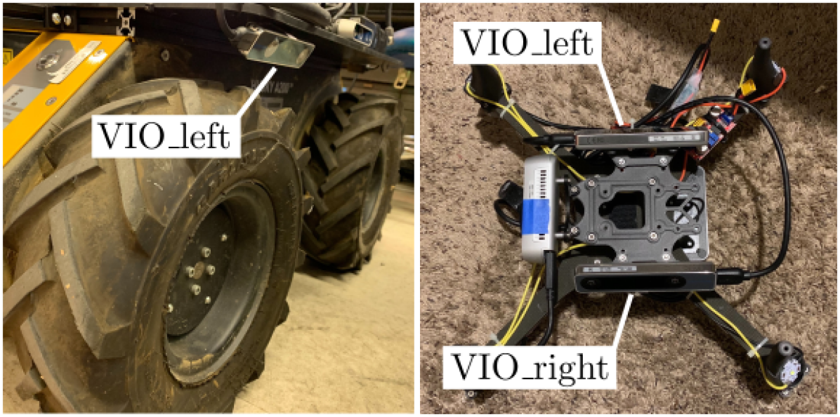
Figure 1: Clearpath Husky robot (left) and NASA-JPL small UAV platform (right and upside down) used in the experiments, both equipped with RealSense T265 camera trackers and Vectornav VN100 inertial measurements units.

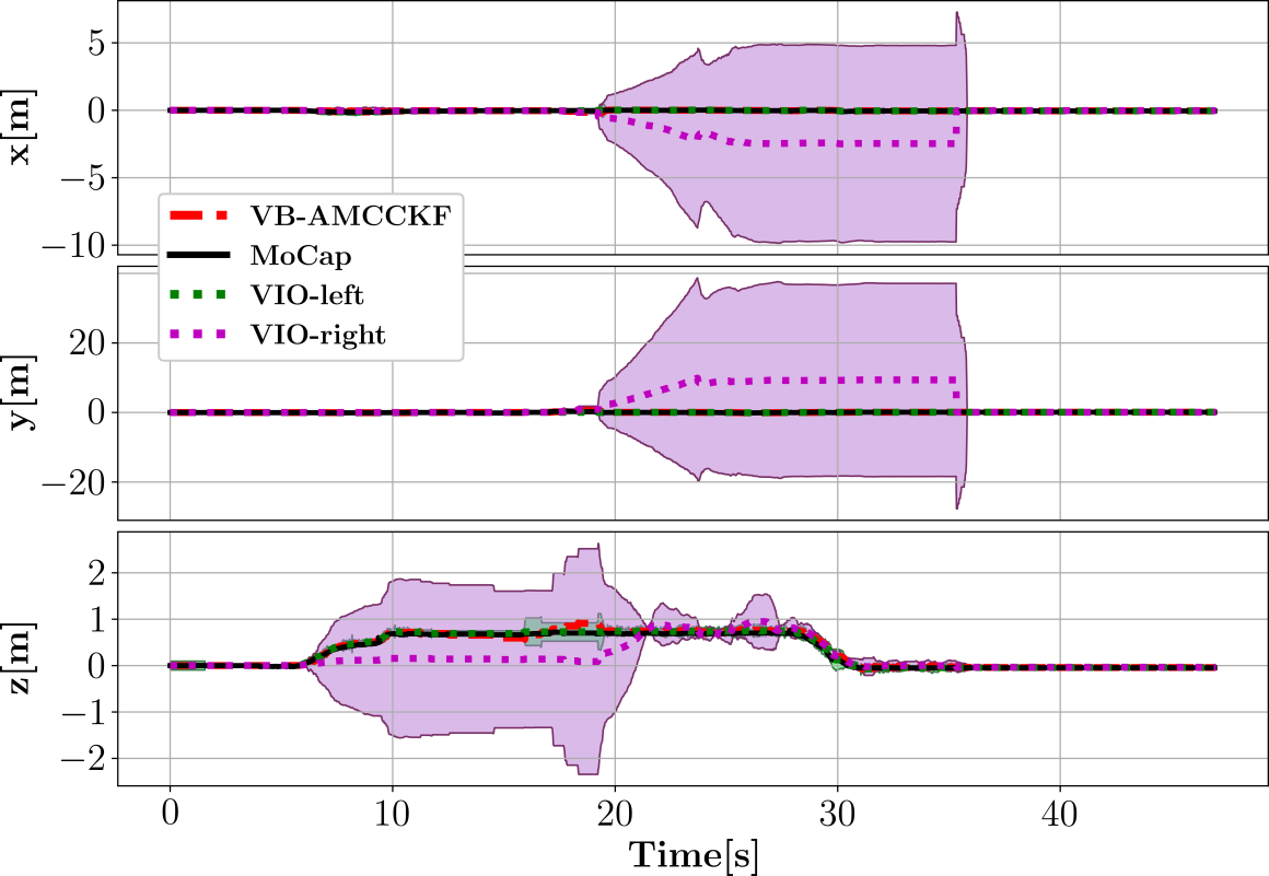
Figure 2: Position estimates from the proposed VB-AMCCKF and the estimated noise covariances for two VIO sources during an indoor flight. Example of tracking degeneracy in the right camera and how the VB-AMCCKF increases the corresponding covariance. The purple and green colored areas correspond to $\pm 3$ times the standard deviations of each tracker (i.e., 3-sigma bands), obtained from their respective $\hat{\mathbf{R}}_{i,k}$.

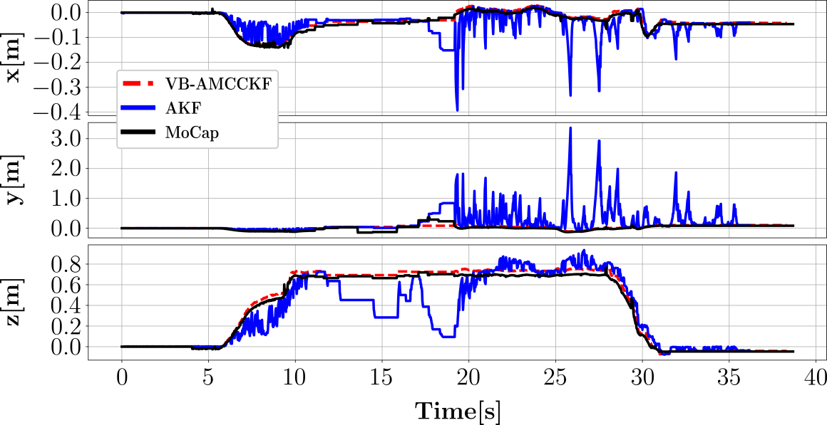
Figure 3: Position estimates from an adaptive EKF (AKF) and the proposed VB-AMCCKF fusing two VIO sources during an indoor flight. Although the AKF has the same adaptive behavior as the VB-AMCCFK, its performance is much worse as seen by the erratic behavior of its estimate. This is attributed to the presence of non-Gaussian noise in the measurements which violates the assumptions of traditional Kalman filters.

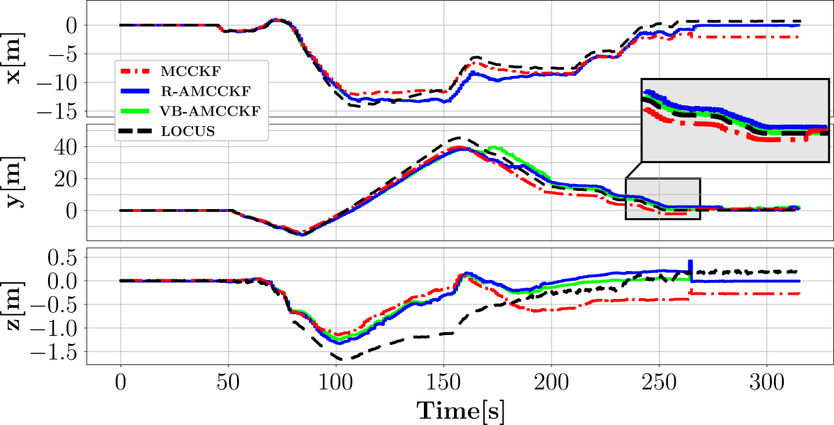
(a) Husky position estimations.

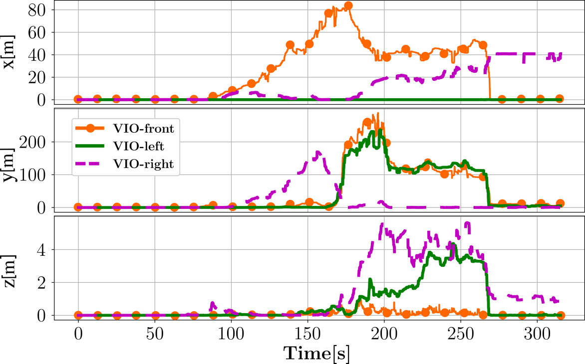
(b) Temporal variation of the adaptive kernel bandwidth (KB) inverse.

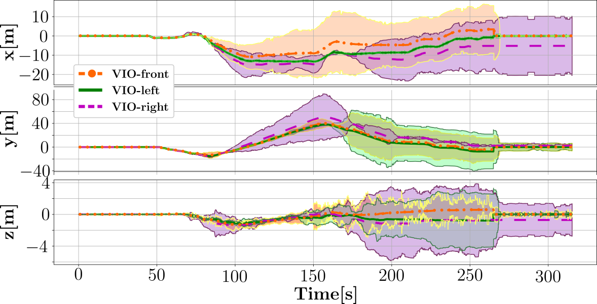
(c) The VIO estimations with their 3-sigma bands from $\hat{\mathbf{R}}_{i,k}$.

Figure 4: The VIO sensors are fused by VB-AMCCKF and R-AMCCKF. The position of the ground robot is shown in (a), $\pm 3$ times of the square root of estimated covariance of each VIO sensors is shown in (b), and the inverse of the adaptive KB is shown in (c). Note that we only show the position of the robot here for the purpose of illustration, however same results hold for rest of the states.

V Experimental Validation

The proposed method was evaluated with real experiments with 1) a small aerial platform (UAV), designed at NASA-JPL and performing indoor flights with fast dynamics and large vibrations; and 2) a Clearpath Husky rover, able to traverse from indoor to outdoor scenarios and navigate large distances. Both robots, shown in Fig. 1, are part of the solution defined by the team COSTAR for the Cave Circuit in the DARPA Subterranean Challenge. Our goal is to produce a smooth state estimate by fusing multiple odometry sources in a loosely-coupled fashion. Commercial-of-the-shelf visual-inertial odometry (VIO) from RealSense – the T265 camera – were mounted to the UAV and ground robot which can be seen in Fig. 1. The UAV had two T265 cameras while the Husky had three; no cameras had overlapping field-of-view so they were treated as independent measurements. Both robots were also equipped with a Vectornav VN100 IMU sensor. The RealSense T265 and Vectonav IMU operate at 200Hz. Note that the gyro and accelerometer biases are not estimated since the VN100 IMU used in the experiments compensates for them internally.

In the following experiments, the kinematic model was propagated with the IMU and corrected with each VIO source. The noise covariance matrix for each camera was initialized to $\hat{\mathbf{R}}_{0}=0.01\times\mathbf{I}_{9}$. In addition, a window size of $\varpi=10$ was chosen for both the VB-AMCCKF and R-AMCCKF. Other parameters for the VB-AMCCKF were set to $\rho=0.97$, $\hat{t}_{0|0}=\hat{b}_{0|0}=0$, $\hat{\mathbf{T}}_{0|0}=\bf 0_{9}$, and $\hat{\mathbf{B}}_{0|0}=\bf 0_{9}$. Even though both platforms carry other sensors, only the 3D LiDAR (Velodyne VLP-16) mounted on the Husky was used for comparison purposes. The following experiments were carried out at the NASA Jet Propulsion Laboratory (JPL).

V-A UAV Experiments

Fig. 2 compares position estimates during a test flight of the UAV from the left and right camera trackers (T265 camera), the VB-AMCCKF approach proposed in this paper, and a Motion Capture (MoCap) system. The robot mainly hovered with a few other maneuvers. In Fig. 2 it is seen that the right camera started to diverge at certain points (possibly cause by poor calibration or few features in the environment). The noise covariance for the right camera (purple area showing $\pm 3\sqrt{\hat{R}_{i,k}}$, with $i\in\{1,2,3\}$) was subsequently increased by the VB-AMCCKF showcasing its ability to identify and adapt to failing sensors. To determine whether only an adaptation behavior is sufficient for these types of scenarios, i.e., removing the MCC component, the VB-AMMCKF was compared to a traditional AKF. Fig. 3 shows that the AKF performs substantially worse than the VB-MCCKF as seen by noisy estimate it generates. It is important to also note that if the AKF estimate were to be used in feedback, the system would become unstable with high probability further highlighting the advantages of the developed approach. An EKF using the same initial noise covariance matrices as in VB-AMCCKF was also evaluated and generated estimates with several meters of error; the results are omitted for plotting clarity. Note, the R-AMCCKF had similar performance to VB-AMCCKF and is omitted for clarity of plotting. The results in Fig. 2 and Fig. 3 showcase the effectiveness of the proposed method to generate smooth and accurate estimates despite the presence of failing or corrupted measurements. Moreover, the combination of robustness – through MCC – and adaptation are the keys to generating robust estimates.

V-B Husky Experiments

Both the VB-AMCCKF and R-AMCCKF methods were also tested on the Husky robot during an experiment where the robot executed a several-meter traverse in an urban environment. In this experiment ground truth from MoCap was not available so the results are compared to a LiDAR-based odometry estimation algorithm called LOCUS [20]. The robot was driven over non-flat terrain to intentionally degrade the performance of the T265 cameras.

Fig. 4(a) first compares the traditional MCCKF (manually tuned with a fixed kernel size and covariance matrices) and the proposed VB-AMCCKF and R-AMCCKF with adaptive KB; the noise covariance matrices were kept static in this test. Here, the traditional MCCKF cannot reach the accuracy of the VB-AMCCKF or R-AMCCKF because the MCCKF lacks adaptive behavior; both VB-AMCCKF and R-AMCCKF generate similar estimates to LOCUS at the end of the trajectory. The inverse of the adaptive KB (Fig. 4(b)) shows the temporal weighting of the sensors in the filter. Smaller values correspond to larger a correntropy gain (i.e, $\mathbf{C}_{k}\rightarrow I$ and more impact in the estimation) and vice versa. Hence, the inverse can be interpreted as a metric for anticipated sensor health; a smaller value corresponds to a sensor that is unlikely to produce an unhealthy measurement, i.e., a healthy sensor. VB-AMCCKF has shown better precision than R-AMCCKF but requiring more computation. We compare the average percentage of the CPU usage between the VB-AMCCKF and R-AMCCKF in Table I. As expected the VB-AMCCKF requires more CPU effort.

As previously stated, one of the advantages of the AMCCKF scheme is the adaptation of the observation noise covariances $\hat{\mathbf{R}}$. Fig. 4(c) shows how the R-AMCCKF adapts for each VIO sensor. The modification of individual dimensions on the covariance matrices allow the AMCCKF to take advantage of the “best” available estimate for each individual dimension. For instance, notice how VIO-left performs best in the estimation for $x$ position, while a combination of front and right cameras prevail for $y$, and VIO-front for $z$. Fig. 4 further demonstrated the effectiveness of the developed VB-AMCCKF and R-AMCCKF.

TABLE I: CPU Usage Comparison.

		Min$\%$	Max$\%$	Avg$\%$	Std$\%$
UAV	R-AMCCKF	30	69	40	12
	VB-AMCCKF	38	81	58	12
Husky	R-AMCCKF	32	74	46	14
	VB-AMCCKF	39	86	65	16

VI Conclusion

This paper proposes two AMCCKF algorithms, based on the Variational Bayesian (VB-AMCCKF) and Residual (R-AMCCKF) techniques, as a step toward robust sensor fusion. The two designs can be selected based on desired accuracy and available onboard computation. Fundamentally, AMCCKF leverage the advantages of MCCKF filters, which show improved robustness with respect to traditional Kalman filters, and extended the design to incorporate adaptive behaviors. The adaptations include a dynamic selection of a) the kernel bandwidth size; b) the system noise covariance matrix; and c) the measurement noise covariance matrix. The addition of online adaptation reduce, the effects of rigid (and usually) inaccurate user-defined parameters. The validity of the proposed filters was demonstrated through real experiments on a UAV and Husky ground robot.

It is worth mentioning some critical points that can drive the AMCCKF to wrong estimations. First, even though the adaptive behaviors for both system and observation noise covariances present clear benefits, there is still some dependency on their initial values which are user-defined. These values, however, may play a role during the initial phase of the experiment, hence when the events are most likely to be under the control of the user (e.g., using a take-off platform or a docking station). Second, the window size ($\varpi$) affects the dynamics of the filter convergence due to the averaging effect, the larger $\varpi$ the slower the convergence. Thus, $\varpi$ should be roughly set according to the vehicle dynamics and the purpose of the estimation. And third, the forgetting factor $\rho$ and the values of the Wishart distribution play a critical role in the performance of the VB-AMCCKF and need to carefully selected (see e.g., [13]. Future work will pursue thorough proofs on the filter stability for both R-AMCCKF and VB-AMCCKF using Lyapunov or contraction-based stability theory.

Appendix A

Residual-based AMCCKF Derivation: From Kalman filtering theory, we can obtain

$${\bm{\Gamma}}_{k}^{-1}\mathbf{y}_{k}=\hat{\mathbf{R}}_{k}^{-1}\mathbf{r}_{k}.$$ (35)

Substituting (35) into (23) and using matrix trace properties, results in

$$\sum_{j=j_{0}}^{k}\text{tr}\left\{\hat{\mathbf{R}}_{j}^{-1}\left[\hat{\mathbf{R}}_{j}\bm{\Gamma}_{j}^{-1}\hat{\mathbf{R}}_{j}-\mathbf{L}_{j}\mathbf{r}_{j}\mathbf{r}_{j}^{\top}\mathbf{L}_{j}\right] \hat{\mathbf{R}}_{j}^{-1}\right\}=0.$$ (36)

Further we also know ([5]) that

$$\mathbf{P}_{k-1|k}\mathbf{H}^{\top}\bm{\Gamma}^{-1}=\mathbf{P}_{k|k}\mathbf{H}^{\top}\hat{\mathbf{R}}_{k}^{-1}.$$ (37)

Left-multiplying both sides of (37) by $\mathbf{H}$ and knowing that the covariance matrix of the innovation is $\bm{\Gamma}_{k}=\mathbf{H}\mathbf{P}_{k|k-1}\mathbf{H}^{\top}+\mathbf{R}_{k}$, we can obtain

$$\left(\bm{\Gamma}_{k}-\hat{\mathbf{R}}_{k}\right)\bm{\Gamma}_{k}^{-1}=\mathbf{H}\mathbf{P}_{k|k}\mathbf{H}^{\top}\bf\hat{\mathbf{R}}_{k}^{-1}.$$ (38)

Then, right-multiplying both sides of (38) by $\hat{\mathbf{R}}_{k}$ and substituting into (36), we have

$$\sum_{j=j_{0}}^{k}\text{tr}\left\{\hat{\mathbf{R}}_{j}^{-1}\left[\hat{\mathbf{R}}_{j}-\mathbf{H}\mathbf{P}_{j}\mathbf{H}^{T}-\mathbf{L}_{j}\mathbf{r}_{j}\mathbf{r}_{j}\top\mathbf{L}_{j}\right] \hat{\mathbf{R}}_{j}^{-1}\right\}=0.$$ (39)

The solution of (39) results in the residual-based adaptive estimation of $\mathbf{R}_{k}$

$$\bm{\Gamma}_{k} =\frac{1}{\varpi}\sum_{j=k-\varpi}^{k}\mathbf{L}_{j}\mathbf{r}_{j}\mathbf{r}_{j}^{\top}\mathbf{L}_{j},$$ (26)

$$\hat{\mathbf{R}}_{k} =\bm{\Gamma}_{k}+\mathbf{H}\mathbf{P}_{k|k}\mathbf{H}^{\top}.$$ (27)

References

- [1] A. M. Zoubir, V. Koivunen, Y. Chakhchoukh, and M. Muma, “Robust estimation in signal processing: A tutorial-style treatment of fundamental concepts,” IEEE Signal Processing Magazine, vol. 29, no. 4, pp. 61–80, 2012.
- [2] A. Santamaria-navarro, R. Thakker, D. D. Fan, B. Morrell, and A. Agha-mohammadi, “Towards resilient autonomous navigation of drones,” in International Symposium on Robotics Research, 2019.
- [3] R. Izanloo, S. A. Fakoorian, H. S. Yazdi, and D. Simon, “Kalman filtering based on the maximum correntropy criterion in the presence of non-gaussian noise,” in IEEE Annual Conference on Information Science and Systems, 2016, pp. 500–505.
- [4] B. Chen, X. Liu, H. Zhao, and J. C. Principe, “Maximum correntropy Kalman filter,” Automatica, vol. 76, pp. 70–77, 2017.
- [5] M. V. Kulikova, “Square-root algorithms for maximum correntropy estimation of linear discrete-time systems in presence of non-gaussian noise,” Systems & Control Letters, vol. 108, pp. 8–15, 2017.
- [6] Y. Huang, Y. Zhang, N. Li, Z. Wu, and J. A. Chambers, “A novel robust student’s t-based Kalman filter,” IEEE Transactions on Aerospace and Electronic Systems, vol. 53, no. 3, pp. 1545–1554, 2017.
- [7] G. Wang, N. Li, and Y. Zhang, “Maximum correntropy unscented Kalman and information filters for non-Gaussian measurement noise,” Journal of the Franklin Institute, vol. 354, no. 18, pp. 8659–8677, 2017.
- [8] M. V. Kulikova, “Chandrasekhar-based maximum correntropy Kalman filtering with the adaptive kernel size selection,” IEEE Transactions on Automatic Control, vol. 65, no. 2, pp. 741–748, 2019.
- [9] S. Akhlaghi, N. Zhou, and Z. Huang, “Adaptive adjustment of noise covariance in Kalman filter for dynamic state estimation,” in IEEE Power Energy Society General Meeting, 2017, pp. 1–5.
- [10] S. Fakoorian, R. Izanloo, A. Shamshirgaran, and D. Simon, “Maximum correntropy criterion Kalman filter with adaptive kernel size,” in 2019 IEEE National Aerospace and Electronics Conference, 2019, pp. 581–584.
- [11] S. Li, B. Xu, L. Wang, and A. A. Razzaqi, “Improved maximum correntropy cubature Kalman filter for cooperative localization,” IEEE Sensors Journal, pp. 1–1, 2020.
- [12] A. Mohamed and K. Schwarz, “Adaptive Kalman filtering for INS/GPS,” Journal of geodesy, vol. 73, no. 4, pp. 193–203, 1999.
- [13] Y. Huang, Y. Zhang, Z. Wu, N. Li, and J. Chambers, “A novel adaptive Kalman filter with inaccurate process and measurement noise covariance matrices,” IEEE Transactions on Automatic Control, vol. 63, no. 2, pp. 594–601, 2017.
- [14] Y. Huang, F. Zhu, G. Jia, and Y. Zhang, “A slide window variational adaptive Kalman filter,” IEEE Transactions on Circuits and Systems II: Express Briefs, 2020.
- [15] A. Agha-mohammadi, K. Otsu, B. Morrell, and et. al., “NeBula: Quest for robotic autonomy in challenging environments; TEAM CoSTAR at the DARPA subterranean challeng,” arXiv preprint arXiv:2103.11470v1, 2021.
- [16] L. Chang and K. Li, “Unified form for the robust gaussian information filtering based on M-estimate,” IEEE Signal Processing Letters, vol. 24, no. 4, pp. 412–416, 2017.
- [17] R. G. Brown, P. Y. Hwang, et al., Introduction to random signals and applied Kalman filtering. Wiley New York, 1992, vol. 3.
- [18] A. Santamaria-Navarro, G. Loianno, J. Solà, V. Kumar, and J. Andrade-Cetto, “Autonomous navigation of micro aerial vehicles using high-rate and low-cost sensors,” Autonomous robots, vol. 42, no. 6, pp. 1263–1280, 2018.
- [19] V. Madyastha, V. Ravindra, S. Mallikarjunan, and A. Goyal, “Extended Kalman filter vs. error state Kalman filter for aircraft attitude estimation,” in AIAA Guidance, Navigation, and Control Conference, 2011, p. 6615.
- [20] M. Palieri, B. Morrell, A. Thakur, K. Ebadi, J. Nash, A. Chatterjee, C. Kanellakis, L. Carlone, C. Guaragnella, and A. Agha-mohammadi, “Locus: A multi-sensor lidar-centric solution for high-precision odometry and 3d mapping in real-time,” IEEE Robotics and Automation Letters, vol. 6, no. 2, pp. 421–428, 2020.