Refractive Light-Field Features for Curved Transparent Objects in Structure from Motion

Abstract

Curved refractive objects are common in the human environment, and have a complex visual appearance that can cause robotic vision algorithms to fail. Light-field cameras allow us to address this challenge by capturing the view-dependent appearance of such objects in a single exposure. We propose a novel image feature for light fields that detects and describes the patterns of light refracted through curved transparent objects. We derive characteristic points based on these features allowing them to be used in place of conventional 2D features. Using our features, we demonstrate improved structure-from-motion performance in challenging scenes containing refractive objects, including quantitative evaluations that show improved camera pose estimates and 3D reconstructions. Additionally, our methods converge 15-35% more frequently than the state-of-the-art. Our method is a critical step towards allowing robots to operate around refractive objects, with applications in manufacturing, quality assurance, pick-and-place, and domestic robots working with acrylic, glass and other transparent materials.

I Introduction

Transparent, or refractive objects are often found in urban settings and industrial applications. However, many robotic vision algorithms find these objects particularly difficult to perceive. Assuming a Lambertian surface—that the appearance of a point on an object does not change with viewpoint—is common, but refractive objects violate this assumption. Their appearance from a particular camera pose is a distorted view of the scene behind them. Thus points on the object’s surface can change dramatically in appearance with small changes in viewpoint. Consequently, robotic vision algorithms, including most approaches to structure-from-motion (SfM) and simultaneous localisation and mapping (SLAM), perform poorly around refractive objects. These algorithms yield incorrect camera trajectories and 3D shape estimates and sometimes fail to converge [1, 2, 3].

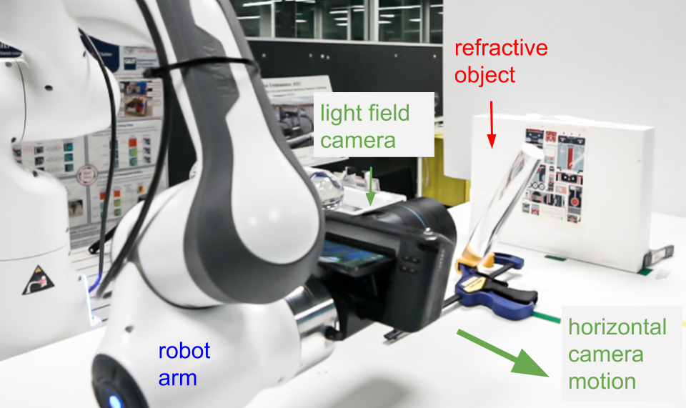
(a)

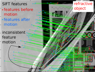
(b)

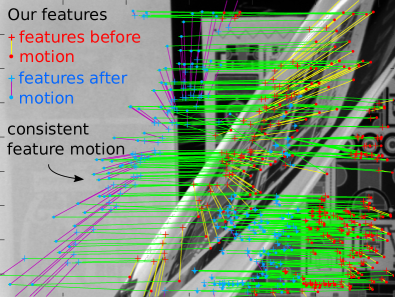
(c)

Figure 1: Comparison of conventional and proposed image features: (a) a robot-mounted LF camera moves horizontally while observing an acrylic cylinder; (b) as seen by the camera, 2D SIFT features’ apparent motion (green) between two frames (from red to blue) is inconsistent across the scene, due to distortion through the refractive object (causing the vertical shift in the refracted image features); (c) the proposed feature exhibits consistent apparent motion (green) between views (only exhibiting horizontal image feature motion), enabling structure-from-motion to operate correctly. The proposed approach yields two characteristic points for refracted features, simplifying to a single point for Lambertian features.

In this work we propose a new feature detector for light field (LF) cameras that allows existing feature-based algorithms to operate in scenes dominated by refractive objects. Image features are distinct points of interest that can be repeatedly and reliably identified from different viewpoints. These form the basis for a range of robotic perception tasks including visual odometry and 3D reconstruction via SfM and SLAM [4]. When image features are visible through an refractive object they exhibit apparent motion inconsistent with the scene geometry and camera trajectory, an example is seen in Fig. 1b. We refer to these as refracted image features. Their view-dependent nature violates assumptions that underpin conventional vision algorithms, which can prevent them from operating as intended [1, 2].

LF cameras are an emerging technology that captures dense and uniformly-sampled multiple views of the scene in one exposure. A single LF image describes view-dependent effects such as occlusion, specular reflection, and in particular, refraction. We exploit this in the context of SfM in a step towards more reliable operation around refractive objects, such as an eye-in-hand robot grasping a transparent wine glass. We propose a method of detecting refracted image features based on the patterns of light passing through curved refractive objects. From these we extract characteristic points with more consistent apparent motion, and show that these can directly enable feature-based algorithms like SfM to operate around refractive objects.

Although previous work has shown LF capture offers advantages in detecting reliable features [5] and ignoring refracted features [2], none has to our knowledge described the detection and use of refracted features for robotic applications. We thus propose a novel feature detector for refractive objects: the refracted light field feature (RLFF). Whereas conventional features identify patterns in the geometry or texture of objects, the RLFF considers the structure of light refracted by refractive objects, finding characteristic points in the free space between objects.

Our key contributions are:

• we describe a new kind of feature, the RLFF, that exists in the patterns of light refracted through objects;

• we propose efficient methods for detecting and extracting RLFF features from LF imagery, and for describing them in terms of characteristic points that can be employed in place of conventional features like SIFT; and

• we demonstrate that using RLFFs improves SfM performance in scenes dominated by refractive objects, yielding more accurate camera trajectory estimates, 3D reconstructions, and more robust convergence, even in complex scenes where state-of-the-art methods otherwise fail.

To evaluate the RLFFs we captured LF imagery using a Lytro Illum camera mounted on a robotic arm. We captured 218 LFs of 20 challenging scenes containing a variety of refractive objects and Lambertian objects. The dataset and code associated with this paper can be accessed at https://tinyurl.com/rlff2021.

Limitations: This work is inspired chiefly by applications dominated by smooth curved objects like drinking glasses and other manufactured transparent items. Evaluation with flat refractive objects is limited, and we expect adaptation of the method may be required. As with any feature-based method, the presence of some texture is required for the algorithm to work. In particular, RLFFs only occur when texture is visible through a refractive object. The approach here will therefore not work with frosted or very complex surfaces through which scene content is not visible. We also assume a geometric ray-based optics approach, so strong defocus effects through highly distorting objects are not considered.

The rest of this paper is organised as follows. We review related work in Section II. In Section III, we discuss the optics of the lens elements that inform the behaviour of our RLFF. Next, the formulation and extraction of our RLFF are described in Section IV. Experimental results using our feature in SfM and comparison to traditional 2D SIFT features are presented and discussed in Section V. Lastly, in Section VI, we conclude the paper and explore avenues for future work.

II Related Work

A variety of approaches for detecting and reconstructing refractive objects using vision have been considered in previous work [1, 6]; however, many require known light sources with bulky configurations that make them impractical for mobile robotics. Other vision-based methods allow for robotic manipulation of refractive objects [7, 8, 9, 10]; however, they rely on having a 3D model of the object a priori. Complete and accurate 3D models and refractive indices of refractive objects are often difficult, time-consuming and expensive to obtain, or simply not available [1]. When such information is not available, localization, manipulation and control of and around refractive objects becomes much harder.

Recently, LF cameras have been considered in the SfM framework [11, 12]. However, these methods employ conventional 2D image features that occur on 3D surfaces. In this paper, we propose a novel 4D feature that is defined by patterns of light that are not necessarily fixed to the surface of an object. We compare our feature to traditional 2D SIFT features in monocular and stereo-based SfM.

For LF-specific features, Tosic et al. developed a type of LF-edge feature [13]; however, our interest is in keypoint features, which tend to be more uniquely identifiable, and are more commonly applied to visual servoing and SfM tasks. Tsai et al. developed the first LF image-based visual servoing algorithm that uses a feature combining central-view image coordinates and depth-dependent LF slope [14]. Teixeira et al. used epipolar planar images (EPIs) to detect reliable Lambertian image features [15]. Similarly, Dansereau et al. proposed the Light-Field Feature (LiFF) detector and descriptor [5], which focused on detecting and describing reliable Lambertian image features in a scale-invariant manner. However, all of these LF features are designed for Lambertian scenes, and are thus not suitable for describing refracted image features.

LFs have been considered for refractive object recognition. Maeno et al. proposed an LF distortion feature (LFD), which modelled an object’s refraction pattern as image distortion [16]. However, the authors observed poor recognition performance due to specular reflections and changes in camera pose. Xu et al. used the LFD as a basis for refractive object image segmentation [3]. Corresponding image features from all views in the LF were fitted to the single normal of a 4D hyperplane using singular value decomposition (SVD). Tsai et al. extended this work to show that a 3D point manifests as a plane in 4D that has two orthogonal normal vectors. This was used to distinguish more types of refractive object, with a higher rate of detection in order to reject refracted scene content [2].

In this paper, we propose a novel RLFF based on the appearance of background texture through a refractive object. We extend existing theory to derive methods for detecting, extracting and estimating the 4D structure of an RLFF in the LF. We use the full LF to detect and extract each feature, making maximal use of available information. We employ the proposed RLFF to allow SfM to operate in scenes dominated by refractive objects. Notably, while prior work focused on detecting and rejecting the refracted scene content, our approach directly uses both the Lambertian and refracted scene content for more reliable camera pose and 3D shape estimation.

III Describing Curved Refractive Objects

We wish to understand the visual appearance of background points imaged through refractive objects, so that we can locally approximate the surface of a refractive object as an astigmatic lens. We begin by investigating the behaviour of light as it travels from the background texture and enters the object. Where the light intersects with the object, the object’s local surface curvature will determine its path, just as in the case of the surface of a lens. In fact, we can describe the entire refractive object as a collection of surface patches, each distorting light based on its local curvature. Fig. 2 illustrates this concept for a toric refractive object, a specific case of an astigmatic refractive object. Here we highlight part of the torus’ surface that has a local shape well described by two orthogonal axes of curvature, each with a corresponding radius of curvature. In the general case of an asymmetric surface, the axes of curvature need not be orthogonal, and the result is an astigmatic surface, part of an astigmatic lens [17].

Other common optical surfaces can be described as special cases of the astigmatic surface. A spherical surface has two identical radii of curvature, and focuses a point source of light to a single point. A cylindrical surface has an infinite radius of curvature in one direction, and focuses a point to a line.

As light leaves the refractive object, it encounters a second surface and is again distorted. As with the first surface, the behaviour is determined by the local curvature of the object. In the general case in which both entrance and exit surfaces are astigmatic, their combined effect is to behave like an astigmatic lens [17].

Fig. 3 depicts the image of a point as it is seen through a general astigmatic lens. Note there are two focal lines at distinct depths $C_{1}$ and $C_{2}$. The shape of the bundle of rays passing through the astigmatic lens is known as an astigmatic pencil. Mathematician Jacques Sturm (1838) investigated the properties of the astigmatic pencil, and it is thus also known as Sturm’s conoid [17]. The shortest line segment connecting the two focal lines is known as the interval of Sturm.

As a line segment, the interval of Sturm can be described by two 3D points. These points have the desirable properties that they can be observed from different positions in the scene, they do not shift significantly as a function of viewpoint, and they can be estimated from a single LF image. These will therefore form the basis for the proposed refractive feature. Though our discussion is concerned with points, generalisation to more complex textural shapes, and in particular the corners or blobs that make up conventional image features, is straightforward.

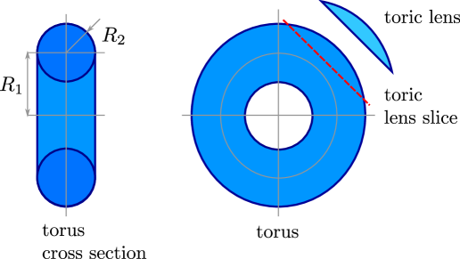
(a)

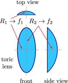
(b)

Figure 2: A complex refractive object can be described in terms of the local curvature of small surface patches. (a) The surface of a torus with radii $R_{1}$ and $R_{2}$ is sliced (dashed red) to form a toric lens surface; (b) The lens surface is defined by two local radii of curvature, and will focus light to focal lines at two distinct focal depths. For the more general astigmatic surface, the axes of curvature need not be orthogonal.

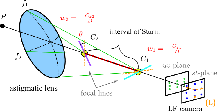
Figure 3: A point $P$ imaged through an astigmatic lens (blue) forms a distorted pencil of rays. Two lines of focus (purple and cyan) form at depths $C_{1}$ and $C_{2}$, and the shortest line connecting these is the interval of Sturm (red). The two 3D points $C_{1}$ and $C_{2}$ that describe the interval of Sturm that comprise our RLFF are shown (yellow/black circles). Observing the scene with an LF camera, we can estimate the orientations of the focal lines and the endpoints of the interval of Sturm. These phenomena are stable with respect to camera pose, and form the basis for our proposed refractive feature.

IV Refracted Light Field Features

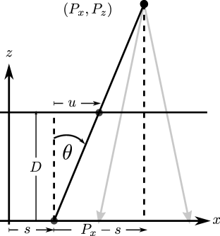
(a)

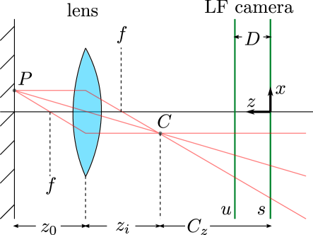
(b)

Figure 4: (a) Geometry of the point-plane correspondence: in a slice of the scene, a Lambertian point $P$ manifests as a line in $s,u$ with slope inversely proportional to $P_{z}$ [18]; the same holds in the $t,v$ dimensions yielding a plane in the 4D LF (1). (b) Imaging the point through an axis-aligned astigmatic lens, in a single slice of the LF, the point $P$ manifests as a focal line going into the page at $C$, yielding a line in $s,u$-space. In a similar slice (not shown), $P$ appears as a second focal line at a different depth (see Fig. 3), yielding a line at a different slope in $t,v$-space; the net result is again a plane, but with unequal slopes for the two slices (2).

Whereas a conventional 2D image feature is defined by a single location in space, e.g. the position of a textural corner or centroid of a blob, the RLFF is more complex, defined by the interval of Sturm, depicted in Fig. 3. This section describes our method for detecting the RLFF and estimating its parameters from a single LF exposure.

We parameterise the LF using the relative two-plane parameterisation [19]. A light ray $\phi$ has coordinates ${\mathitbf{\phi}}=[s,t,u,v]$, where $s,t$ and $u,v$ describe the points of intersection with two reference planes separated by an arbitrary distance $D$, and $s,t$ are chosen to be further from the scene as depicted in Figs. 3, 4. In the relative parameterisation, $u,v$ are expressed relative to $s,t$. In the sampled LF, we employ the discrete variables $i,j,k,l$, where $i,j$ select a sub-image, and $k,l$ select a pixel from that image.

IV-A Feature Detector and Descriptor

There is an opportunity to exploit the local 4D structures of light refracted through objects to define a unique feature detector and descriptor. However, for this work we are focused chiefly with identifying and extracting the parameters of refractive features. We therefore leverage existing 2D tools to detect and describe RLFF features. In an approach similar to [11] and [15], we apply a SIFT detector to each sub-image of the LF, then match these between views. We employ Root SIFT descriptors applied to the central sub-image of the 2D feature for more reliable matching [20], and match between LF sub-images based on the Euclidean distance between descriptors. Only allowing features that match across a minimum number of sub-images allows us to reject spurious detections. In future work, we envision extending a direct LF feature detector like LiFF, which detects features by simultaneously considering the entire LF [5].

The detection process yields a set of discrete-space observations $\bm{n}$, each of the form $\bm{n_{i}}=[i,j,k,l]$ corresponding to the centroid of the detected SIFT feature $k,l$ in each sub-image $i,j$. This approach works in the presence of refractive features because, although textural blobs have distorted apparent motion in the LF, their appearance is very similar across the LF sub-images, particularly for small-baseline cameras like the hand-held Lytro employed in this work.

Next, to effectively estimate the interval of Sturm and extract the feature’s parameters, we require that the sub-images observing the feature have sufficient diversity. If we consider the LF as a grid of sub-images, a line of sub-images from this grid does not suffice to observe astigmatic refractions. Views must subtend a 2D space. To evaluate view diversity, we use the coefficient of determination $R^{2}$ of a line of best fit from the $s,t$ coordinates of matching views. High coefficients of determination correspond to a mostly linear set of views, and we empirically determined $R^{2}>0.65$ to be a suitable criterion for rejection.

IV-B Feature Extraction

In this section we describe the process of estimating the parameters of the RLFF. The feature detection yields a set of observations in discrete space $\bm{n_{i}}$. We begin by converting this to a continuous-domain representation by calibrating the camera to yield an LF intrinsic matrix [21]. This allows us to convert each observation $\bm{n_{i}}$ to a continuous-domain ray $\bm{\phi_{i}}=[s,t,u,v]$.

In the case of a Lambertian scene point, it is well established that the set of observations $\bm{\phi}$ will lie on a plane in the 4D light field [18]. The geometry for this point-plane correspondence is depicted in Fig. 4a, and is given by

$$\begin{bmatrix}u\\ v\end{bmatrix}=\begin{pmatrix}-\frac{D}{P_{z}}\end{pmatrix}\begin{bmatrix}s-P_{x}\\ t-P_{y}\end{bmatrix}.$$ (1)

This can be interpreted as the intersection of two hyperplanes, where the slopes of the hyperplanes in the epipolar plane dimensions $s,u$ and $t,v$ are identical, given by $-D/P_{z}$.

We now generalise the point-plane correspondence by introducing an astigmatic lens between the camera and the Lambertian point, as depicted in Fig. 4b. We initially assume a thin toric lens with axes aligned with the $s$ and $t$ axes. This yields two orthogonal lines of focus at depths $P_{z1},P_{z2}$. In $s,u$ the behaviour is similar to that of a Lambertian point at depth $P_{z1}$, whereas in $t,v$ the rays appear to emerge from a point at depth $P_{z2}$. We can write this more formally as

$$\begin{split}\begin{bmatrix}u\\ v\end{bmatrix}=&S\begin{bmatrix}s-P_{x}\\ t-P_{y}\end{bmatrix},\quad S=\begin{bmatrix}-D/P_{z1}&0\\ 0&-D/P_{z2}\end{bmatrix},\end{split}$$ (2)

where $P_{z}$ are apparent depths corresponding to the extremities of the interval of Sturm.

For the more general case of non-camera-aligned lines of focus, i.e. the case of a general astigmatic lens, we apply a transformation

$$\begin{split}\begin{bmatrix}u\\ v\end{bmatrix}=&H\begin{bmatrix}s-P_{x}\\ t-P_{y}\end{bmatrix},\quad H=VSV^{\text{-}1},\end{split}$$ (3)

where $V$ is a rotation matrix for the special case of a rotated toric lenses, and the concatenation of two potentially non-orthogonal axes $[V_{1},V_{2}]$ for a general astigmatic lens. This transformation assumes the interval of Sturm is close to parallel with the principal axis of the camera, an assumption that holds well under most of the imaging scenarios we consider, in which features must be visible through the refractive object.

Finally, separating the translation terms yields the generalised point-plane correspondence for points imaged through astigmatic lenses

$$\begin{split}\begin{bmatrix}u\\ v\end{bmatrix}=&H\begin{bmatrix}s\\ t\end{bmatrix}+X,\quad X=-H\begin{bmatrix}P_{x}\\ P_{y}\end{bmatrix}.\end{split}$$ (4)

Note that this general form also describes the Lambertian case, for which the depths $P_{z1}$ and $P_{z1}$ are identical and (4) degenerates to (1).

IV-C Estimating Feature Parameters from Observations

From (4), observations of a scene point take the form

$$\begin{split}\begin{bmatrix}u\\ v\end{bmatrix}=\begin{bmatrix}h1&h2&x1\\ h3&h4&x2\end{bmatrix}\begin{bmatrix}s\\ t\\ 1\end{bmatrix}.\end{split}$$ (5)

Given a set of $[s,t,u,v]$ observations for a single feature, we find the least squares solution to (5), directly yielding estimates $\hat{H}$ and $\hat{X}$.

Eigenvalue decomposition of $\tilde{H}$ allows us to estimate $V$ and $S$ following (3). Equating terms from (2)–(4) allows us to solve for $P_{x},P_{y},P_{z1},P_{z2}$ as well as the directions of the axes $V_{1}$ and $V_{2}$, $\theta_{1}$ and $\theta_{2}$, respectively. These are the parameters of the focal lines caused by an astigmatic lens and the interval of Sturm. These six parameters also compose our definition of the Refracted Light Field Feature (RLFF):

$$RLFF=\begin{bmatrix}P_{x},P_{y},P_{z1},P_{z2},\theta_{1},\theta_{2}\end{bmatrix}.$$ (6)

Though physically realizable $H$ matrices are symmetric, the estimate $\hat{H}$ may not be. Asymmetric matrices can result in imaginary eigenvalues. Prior to eigendecomposition we force $\hat{H}$ to be symmetric, $\hat{H}_{S}=(\hat{H}+\hat{H}^{T})/2$, where ^T is the matrix transpose. We note that using a constrained least squares estimator would likely yield improved noise performance.

When estimating the offsets, $P_{x}$ and $P_{y}$, we use the reconstructed $H_{\scriptscriptstyle\mathit{R}}=VSV^{\text{-}1}$ rather than $\hat{H}$, as this improves noise performance. The residual between $\hat{H}$ and $H_{\scriptscriptstyle\mathit{R}}$ forms a convenient indicator for outlier features not well described by our assumptions.

An example of a feature extracted from captured LF imagery is shown in Fig. 5. The sub-image views are shown in blue, the set of $s,t,u,v$ observations across the LF are shown in gray, and the estimated focal lines and interval of Sturm are shown as coloured line segments.

IV-D Driving SfM

The proposed feature definition comprises two infinite lines of focus and the interval between them. We anticipate constructing robotic vision algorithms that work directly off these features. However, existing systems like the popular SfM solution COLMAP [22] accept only 2D image features like SIFT. Thus, we propose two mechanisms for driving existing vision systems with the proposed feature for comparison with monocular- and stereo-based SfM approaches.

First, by projecting the 3D endpoints of the interval of Sturm into the central view of the camera, they are reduced to 2D image features. This RLFF mono has the drawback of discarding all 3D information associated with the feature. Second, we therefore propose a variation of this approach in which we instead project the same endpoints into two separate LF views, separated by a baseline similar to that of the LF camera. This RLFF stereo preserves most of the 3D information of the feature, discarding only the orientations of the focal lines. This also preserves our knowledge of the baseline over which depth is being estimated, an important detail for reconstruction algorithms that consider uncertainty associated with short-baseline depth estimates. We evaluate both variations of this approach in Section V.

Note that our approach simultaneously detects both Lambertian and refracted features, and passes them all into SfM. Lambertian scene points yield a zero-length interval of Sturm, and so appear as a single point rather than as a pair. This is visible in our results, e.g. see the refracted and background Lambertian features in Fig. 1c.

Many applications will benefit by distinguishing Lambertian and refracted features, as Lambertian points generally correspond to an object’s surface, while refracted features are images that exist in free space. Prior work has distinguished refracted features on the basis of slope differences in 3D subsets of the LF [2]. The RLFF effectively measures how Lambertian an image feature is in a more complete way, as the entire LF is employed. The interval of Sturm is of zero length for Lambertian scene points, and only takes on finite extent for refracted scene content.

Note also that in the case of refracted features we are passing two characteristic points to COLMAP as though they were separate 2D features. We require a descriptor for each of these to allow feature matching, but wish to disallow matching of front and back characteristic points $C_{1}$ and $C_{2}$ between frames. To this end we propose three approaches. First, the descriptor can be modified to reflect which focal line it belongs to, front or back, e.g. through addition of a bias term, scaling factor, of by raising to some power. Then matches could not occur between front and back features as their descriptors differ substantially. Second, one can perform matching externally to the SfM tool while keeping track of which characteristic point each feature corresponds to. Then potential matches between front and back points are simply not evaluated. Finally, the approach taken in this work is to employ identical descriptors for the two points, yielding extraneous putative matches, and relying on outlier detection to reject these on the basis of epipolar geometry.

V Evaluation

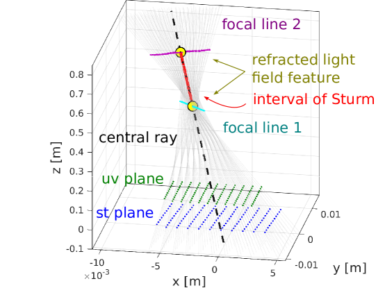
Figure 5: An RLFF extracted from Illum imagery. The $st$ sub-images (blue) and $uv$ observations (green) are shown from distance $D=0.1m$ from the $st$-plane. The rays projected by $stuv$ (grey) pass through both the first and second focal lines (cyan and magenta, respectively). The central ray of the feature is shown (dashed black). The interval of Sturm (red), and the two 3D points (yellow) define our RLFF.

	SIFT	RLFF
Wine glass
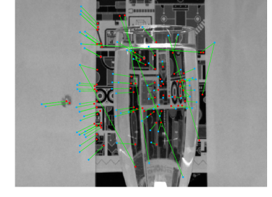
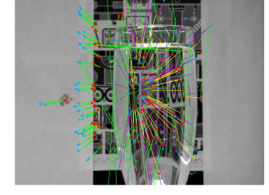
Sphere
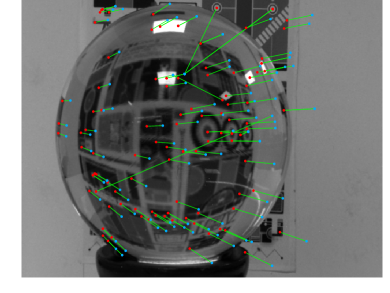
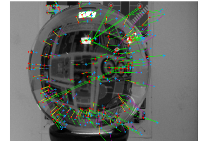
Cylinder

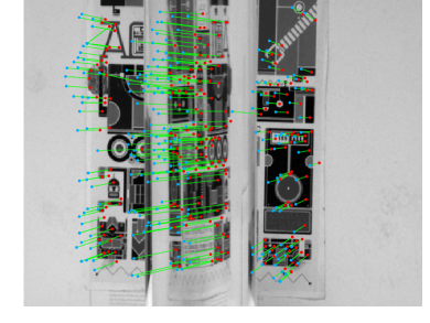
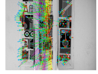
Figure 6: Three example scenes for which COLMAP fails when using SIFT features (left) but succeeds when using the proposed RLFF. These examples also show different types of camera motion: the wine glass has forwards motion, the sphere has horizontal motion, and the cylinder has both. The proposed features show some inconsistent apparent motion near the edges of the refractive objects; however their motion is more consistent than SIFT, allowing COLMAP to converge.

To evaluate the proposed feature we mounted an Illum LF camera on a Franka Emika Panda robot arm. The LF camera was calibrated using the LF Toolbox [21]. To reduce the effect of extreme lens distortion, we cropped the $15\times 15$ LF to a $13\times 13$ array of sub-images. The robot arm was used for repeatability and ground truth trajectories with sub-millimeter positional accuracy. We used a variety of refractive objects, such as a water bottle, glass sphere, glass cups filled with water, combined with a variety of textured backgrounds. The experimental setup is illustrated in Fig. 1a.

V-A Structure from Motion

To evaluate the RLFF, we used the popular COLMAP SfM implementation [22]. Following the procedure outlined in Section IV-D, we converted each detected RLFF to a pair of 2D image features, as seen from the central view of the LF camera (the middle view of a LF if we consider the LF as a grid of views). We also evaluated the alternative approach of projecting the feature into a stereo pair of LF views, preserving depth information.

For comparison, we evaluated conventional SIFT features as seen in the central LF view. To better understand the impact of projecting features into stereo pairs, we also compared with SIFT similarly projected into a pair of LF views, with the same baseline as for the RLFF test. In all, we compared four methods using COLMAP, covering the proposed RLFF and SIFT for both monocular and stereo views: RLFF mono, RLFF stereo, SIFT mono and SIFT stereo.

We evaluated performance using COLMAP’s sparse SfM. SfM was not able to reconstruct all scenes for all types of objects, as its solution did not always converge. This was especially problematic for scenes dominated by refracted content. Following [5] and [22], we evaluated peformance in terms of the percentage of scenes for which COLMAP converged, the number of image features per image, putative image feature matches per image, inlier matches per image during SfM, putative match ratio, mean number of 3D points, track length, precision and matching score. The putative match ratio is the proportion of detected image features that yielded putative matches. The mean number of 3D points in the reconstructed models serves as an indicator of how many features were stable enough to be included into the model. The track length is the mean number of camera poses over which a feature was successfully tracked. The precision is the proportion of putative image feature matches that yielded inlier matches. The matching score is the proportion of image features that yielded inlier matches. Note that for the RLFF features, we divided the number of image features, putative matches, inlier matches and 3D points by two because a single RLFF is represented by a pair of points, the extents of the interval of Sturm. Similarly, we divided the track length by two for both stereo approaches, as twice the number of images were considered during the motion sequences. This yielded more meaningful quantitative comparison.

We collected 20 sequences consisting of 10 to 20 camera poses each, covering a variety of motion trajectories and a diverse set of scene content including spherical, cylindrical, and general astigmatic elements. The dataset contains 218 LFs in total. Example images highlighting the differences between SIFT and RLFF performance are shown in Fig. 6. In all of these scenes COLMAP was unable to converge while using either version of SIFT, but succeeded when using our RLFF.

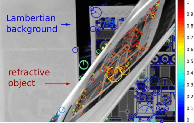
Figure 7: Identifying features as Lambertian or refracted. Features are coloured to indicate the extent to which they have consistent slopes following (1). Warmer colours indicate very inconsistent slopes and thus refracted features. Some inconsistencies are observed along occlusion boundaries and image borders (green/turquoise features), due to the apparent slope inconsistencies these induce in the LF.

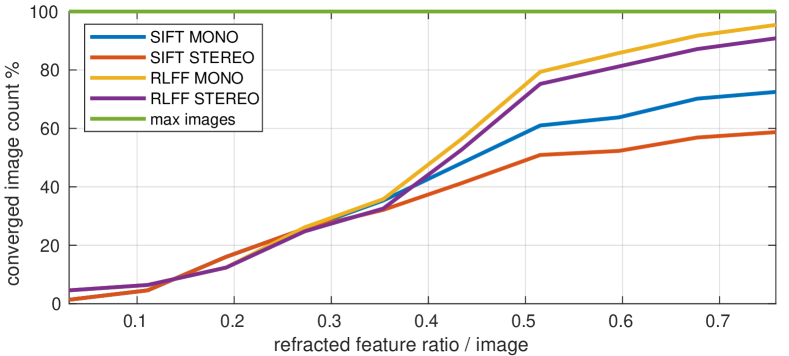
Figure 8: Cumulative histogram of imagery successfully incorporated into the COLMAP SfM model (as a percent of 218 LFs) versus the refracted scene content in the image. Toward the right of the figure, imagery becomes increasingly challenging as more of the image features become refracted and fewer images are being incorporated by each SfM solution, especially for the SIFT-based solutions. An ideal method would incorporate all images, ending with a value of 100 %, being able to incorporate all of the imagery. Our RLFF-based SfM reconstructs more images in total, showing the strongest advantage with more refracted content.

[caption = Evaluating the proposed RLFF and SIFT in SfM, both in monocular and stereo modes. More scenes converge using the proposed method, and it outperforms the state-of-the-art in all measures except precision., label = tbl:sfmFeatureStats, doinside = , star ] lccccccccccc Methods & # LF s % # LF s Image Putative Inlier Putative 3D Track Precision Matching
converged Pass common Features Matches Matches Match Points Length Score
/ Img / Img / Img Ratio SIFT MONO 158 0.75 118 372 122 112 0.369 431 5.11 0.916 0.340
SIFT STEREO 128 0.6 118 370 131 122 0.369 524 4.16 0.922 0.342
RLFF MONO 208 0.95 118 321 155 134 0.448 437 5.27 0.842 0.385
RLFF STEREO 198 0.9 118 321 168 147 0.487 684 4.04 0.863 0.426

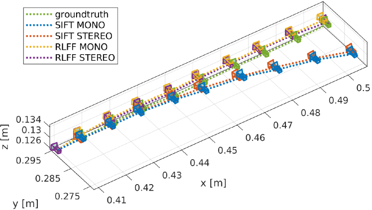
(a)

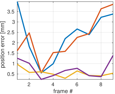
(b)

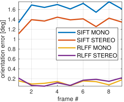
(c)

Figure 9: Comparing pose accuracy in a trajectory that approaches a refractive object, making images progressively more difficult due to increasing refractive scene content: (a) Estimated trajectories show both proposed stereo and mono variants of RLFF outperforming both variants of SIFT; (b) Relative, instantaneous translational and (c) rotational error show the proposed methods outperforming SIFT in all cases.

To understand how refractive objects affect SfM performance, we evaluated the extent to which each LF is dominated by refractive features. We took the extent of the interval of Sturm for each feature as an indication of how Lambertian it is. Lambertian scene points evaluated by our feature extractor yield an interval of Sturm of zero length, or equivalently, correspond to a plane with equal slopes in horizontal and vertical dimensions following (1). Fig. 7 shows an example.

A limitation of this approach is that it does not work for spherical lenses, which produce a well-formed image that behaves identically to Lambertian scene content. Human viewers are also susceptible to this, and it is the basis for some display technologies that produce images floating in air. Features refracted through spherical objects are thus not well detected by our method. They do, however, make excellent points for use in SfM, so while we do not detect them as being refracted, we do make use of them in the SfM solution.

We plotted the number of images correctly incorporated into an SfM solution by COLMAP. By sorting images on the horizontal axis according to the fraction of features identified as refractive (i.e. the refracted feature ratio), we obtain the cumulative histogram shown in Fig. 8. This shows both variants of the proposed method enabled SfM to succeed with almost all images, while the SIFT-based methods failed to converge for a significant number. Importantly, the difference in performance is due chiefly to scenes dominated by refracted content.

V-B 3D Reconstruction Performance

We ran COLMAP across all of the collected scenes, and summarise the results in Table LABEL:tbl:sfmFeatureStats. The statistics show that RLFF methods have a higher proportion of putative and inlier matches, the number of 3D points in the reconstructions, the track length, and the overall matching score. Our methods converged 15-35% more frequently than their SIFT counterparts, and performed better in almost all measures except precision. The stereo version of RLFF generally showed higher performance, though the monocular version allowed more scenes to converge. We explain weaker precision performance of RLFF by noting more putative matches due to doubling the number of 2D image features, which subsequently quadrupled the number of potential 2D feature matches. In this preliminary work, descriptors were only duplicated for the RLFF projections to 2D image features. For refracted image features, the distance between feature projections was sufficiently large to discriminate. However, for Lambertian features where the projections are coincident, we increased the putative matches without increasing the inliers. This resulted in lower precision. To prevent this issue, we can adopt the strategies proposed earlier in Sec. IV-D for future work. Overall, these results showed that the proposed RLFF feature allowed COLMAP to operate in many scenes for which it could not previously operate.

V-C Camera Trajectory Estimation

We also evaluated the accuracy of camera trajectories estimated by SfM. Ground truth was available by virtue of our use of a robotic arm to carry out the camera trajectories. A comparison of camera trajectory estimates and their corresponding translational and rotation error are shown in Fig. 9. For this scene, the proposed RLFF feature showed substantially higher performance in both rotational and translational error, yielding a much more accurate trajectory estimate.

[caption = Comparison of relative, instantaneous pose error using monocular and stereo RLFF and SIFT. The proposed RLFF allowed almost all sequences to converge, while SIFT did not. The proposed feature outperformed SIFT both on the easier sequences in which all methods converged (top), and in the more challenging sequences (bottom)., label = tbl:SfMcomparison, doinside = ] cc cc cc cc cc SIFT SIFT RLFF RLFF
MONO STEREO MONO STEREO
Seq. #LFs $e_{tr}$ [mm] $e_{rot}$ [deg] $e_{tr}$ $e_{rot}$ $e_{tr}$ $e_{rot}$ $e_{tr}$ $e_{rot}$ 1 10 1.37 0.40 1.34 0.40 2.64 0.20 1.03 0.19
2 10 1.22 0.27 1.44 0.29 2.36 0.28 1.58 0.21
3 10 16.50 6.86 2.08 0.11 5.83 0.29 2.51 0.23
4 10 1.99 0.14 2.12 0.13 1.26 0.13 2.17 0.15
5 10 2.35 1.62 2.22 1.35 0.55 0.12 0.73 0.14
6 10 0.84 0.47 2.97 0.42 0.93 0.42 3.07 0.43
7 10 1.60 1.52 4.02 2.65 0.92 0.17 2.38 1.78
8 10 4.21 0.60 4.69 0.53 7.20 0.71 3.63 0.38
9 10 5.82 1.53 5.71 1.26 5.43 0.78 15.49 2.88
10 18 2.21 0.97 6.97 1.91 1.42 0.78 9.47 3.34
11 10 24.44 8.51 24.38 7.38 7.87 0.69 1.98 0.34 Mean - 5.69 2.08 5.27 1.49 3.31 0.42 4.00 0.92 12 10 7.24 2.85 7.90 3.01 1.87 1.33 - -
13 10 1.54 0.26 - - - - - -
14 10 7.13 1.23 - - 14.70 0.48 1.87 0.16
15 10 2.30 0.62 - - 1.75 0.36 2.65 0.50
16 10 - - - - 1.19 0.45 1.31 0.34
17 20 - - - - 1.39 0.19 1.15 0.15
18 10 - - - - 3.27 0.36 2.09 0.27
19 10 - - - - 3.14 0.38 1.99 0.29
20 10 - - - - 2.66 0.33 2.01 0.29

Mean - 4.55 1.24 7.90 3.01 3.75 0.48 1.87 0.29

A summary of pose accuracy over all the test scenes is shown in Table LABEL:tbl:SfMcomparison, shown in terms of the mean instantaneous pose error, and comparing the same four variants of SIFT and RLFF-based approaches as before. We separate scenes for which all methods converged, allowing direct comparison of statistics in the top half of the table, but noting that these correspond to the easiest scenes. Overall, the monocular variant of RLFF showed the strongest performance for these easier scenes; whereas, the stereo version performed better for the more challenging scenes, in which at least one method failed to converge.

Overall, these results show the proposed methods outperforming SIFT-based methods, and importantly, the proposed method converged in all scenes but one (mono) or two (stereo), while the SIFT-based methods failed to converge for five (mono) or eight (stereo). We see the proposed method allows SfM to operate in scenes where it previously could not, but also that it improves performance in camera pose estimation wherever these is refracted scene content, even for less challenging scenes.

VI Conclusions

In conclusion, we proposed a novel 4D feature defined by the rays of light travelling through curved refractive objects, as opposed to the conventional 2D image features defined by a single 3D point in space. Advantageously, our feature captures both Lambertian points and features imaged through smooth refractive objects. We demonstrated methods for detecting and extracting the proposed RLFF from LF imagery captured by a hand-held LF camera, and for employing the resulting features in conventional vision algorithms including SfM. Finally, we evaluated RLFF’s benefits in the context of SfM, comparing to conventional SIFT-based methods. We showed the proposed method allowed SfM to operate where it could previously could not. We also show improved 3D reconstruction performance and 3D camera trajectory estimation. Our method is especially advantageous in scenes dominated by refractive object s, in which traditional approaches fail.

For future work, we intend to develop a feature detector and descriptor that directly employ the local 4D structure of refracted features, as in the LiFF feature for Lambertian LFs [5]. Demonstrating RLFF in more scenarios is also of interest, including closed-loop control for visual servoing, and place recognition for localisation and SLAM. Finally, it is well understood that reflection off smooth curved surfaces exhibits characteristics similar to refraction through transparent objects. We expect generalisation of the RLFF to reflective scenes to be straightforward and to show similar performance advantages as in the refractive case.

References

- [1] I. Ihrke, K. Kutulakos, H. Lensch, M. Magnor, and W. Heidrich, “Transparent and specular object reconstruction,” Computer Graphics forum, vol. 29, pp. 2400–2426, 2010.
- [2] D. Tsai, D. G. Dansereau, T. Peynot, and P. Corke, “Distinguishing refracted features using light field cameras with application to structure from motion,” IEEE Robotics and Automation Letters (RA-L), vol. 4, no. 2, pp. 177–184, April 2019.
- [3] Y. Xu, H. Nagahara, A. Shimada, and R. ichiro Taniguchi, “Transcut: Transparent object segmentation from a light field image,” Intl. Conference on Computer Vision and Pattern Recognition (CVPR), 2015.
- [4] P. Corke, Robotics, Vision and Control. Springer, 2013.
- [5] D. G. Dansereau, B. Girod, and G. Wetzstein, “LiFF: Light field features in scale and depth,” in CVPR, 2019, pp. 8042–8051.
- [6] D. Miyazaki and K. Ikeuchi, “Inverse polarisation ray-tracing: estimating surface shapes of transparent objects,” CVPR, 2005.
- [7] C. Choi and H. Christensen, “3D textureless object detection and tracking: An edge-based approach,” in Intl. Conference on Intelligent Robots and Systems (IROS), 2012.
- [8] C. Walter, F. Penzlin, E. Schulenburg, and N. Elkmann, “Enabling multi-purpose mobile manipulators: Localization of glossy objects using a light field camera,” in Conference on Emerging Technologies & Factory Automation (ETFA). IEEE, 2015, pp. 1–8.
- [9] I. Lysenkov, “Recognition and pose estimation of rigid transparent objects with a kinect sensor,” Robotics: Science and Systems VIII, p. 273, 2013.
- [10] Z. Zhou, Z. Sui, and O. C. Jenkins, “Plenoptic Monte Carlo object localization for robot grasping under layered translucency,” in IROS. IEEE, 2018, pp. 1–8.
- [11] O. Johannsen, A. Sulc, and B. Goldluecke, “On linear structure from motion for light field cameras,” in Intl. Conference on Computer Vision (ICCV), 2015, pp. 720–728.
- [12] S. Nousias, M. Lourakis, and C. Bergeles, “Large-scale, metric structure from motion for unordered light fields,” in CVPR, 2019, pp. 3292–3301.
- [13] I. Tosic and K. Berkner, “3D keypoint detection by light field scale-depth space analysis,” in Image Processing (ICIP). IEEE, 2014.
- [14] D. Tsai, D. G. Dansereau, T. Peynot, and P. Corke, “Image-based visual servoing with light field cameras,” RA-L, vol. 2, no. 2, pp. 912–919, 2017.
- [15] J. A. Teixeira, C. Brites, F. Pereira, and J. Ascenso, “Epipolar based light field key-location detector,” in Multimedia Signal Processing. IEEE, 2017.
- [16] K. Maeno, H. Nagahara, A. Shimada, and R. Taniguchi, “Light field distortion feature for transparent object recognition,” in CVPR. IEEE, Jun. 2013.
- [17] E. Hecht, Optics, 4th ed. Addition-Wesley, 2002.
- [18] E. H. Adelson and J. Y. A. Wang, “Single lens stereo with a plenoptic camera,” IEEE Transactions on Pattern Analysis & Machine Intelligence, no. 2, pp. 99–106, 1992.
- [19] M. Levoy and P. Hanrahan, “Light field rendering,” in SIGGRAPH. ACM, 1996, pp. 31–42.
- [20] R. Arandjelović and A. Zisserman, “Three things everyone should know to improve object retrieval,” in CVPR. IEEE, 2012, pp. 2911–2918.
- [21] D. G. Dansereau, O. Pizarro, and S. B. Williams, “Decoding, calibration and rectification for lenselet-based plenoptic cameras,” in CVPR. IEEE, Jun. 2013, pp. 1027–1034.
- [22] J. Schoenberger and J.-M. Frahm, “Structure-from-motion revisited,” CVPR, 2016.