Local well-posedness for the Zakharov system in dimension $d=2,3$

Abstract: The Zakharov system in dimension $d=2,3$ is shown to have a local unique solution for any initial values in the space $H^{s}\times H^{l}\times H^{l-1}$, where a new range of regularity $(s,l)$ is given, especially at the line $s-l=-1$. The result is obtained mainly by the normal form reduction and the Strichartz estimates.

Keywords: Zakharov; local well-posedness; normal form reduction; strichartz estimate

1 Introduction

The initial-value problem for the Zakharov system is:

$$\left\{\begin{array}[]{l}i\dot{u}-\Delta u=nu,\\ \ddot{n}/\alpha^{2}-\Delta n=-\Delta|u|^{2},\\ u(0,x)=u_{0}(x),n(0,x)=n_{0}(x),\dot{n}(0,x)=n_{1}(x).\end{array}\right.$$ (1.1)

Here, $u(t,x):\mathbb{R}\times\mathbb{R}^{d}\longmapsto\mathbb{C},n(t,x):\mathbb{R}\times\mathbb{R}^{d}\longmapsto\mathbb{R}.$ $\alpha>0$ is called the ion sound speed. This problem arises in plasma physics. Sufficiently regular solutions of $\eqref{1.1}$ satisfy the conservation of mass

$$\int_{\mathbb{R}^{d}}|u|^{2}dx=\int_{\mathbb{R}^{d}}\left|u_{0}\right|^{2}dx$$ (1.2)

and conservation of the Hamiltonian

$$E=\int_{\mathbb{R}^{d}}|\nabla u|^{2}+\frac{\left|D^{-1}\dot{n}\right|^{2}/\alpha^{2}+|n|^{2}}{2}-n|u|^{2}dx,$$ (1.3)

where $D:=\sqrt{-\Delta}$. The Zakharov system is typically studied as a Cauchy problem by prescribing initial data in the space

$$\left(u_{0},n_{0},n_{1}\right)\in H^{s}\left(\mathbb{R}^{d}\right)\times H^{l}\left(\mathbb{R}^{d}\right)\times H^{l-1}\left(\mathbb{R}^{d}\right).$$ (1.4)

In terms of $N:=n-iD^{-1}\dot{n}/\alpha$, we can change the system $\eqref{1.1}$ into first order as usual:

$$\left\{\begin{array}[]{l}\left(i\partial_{t}-\Delta\right)u=Nu/2+\bar{N}u/2,\\ \left(i\partial_{t}+\alpha D\right)N=\alpha D|u|^{2},\\ u(0,x)=u_{0}(x),N(0,x)=N_{0}(x),\end{array}\right.$$ (1.5)

where $\left(u_{0},N_{0}\right)\in H^{s}\left(\mathbb{R}^{d}\right)\times H^{l}\left(\mathbb{R}^{d}\right)$. Since the term $\bar{N}u$ makes no essential difference from $Nu$, from here on out, we will replace the nonlinear term $Nu/2+\bar{N}u/2$ with $Nu$.

The system $\eqref{1.1}$ was introduced by Zakharov [18] to depict the Langmuir turbulence in unmagnetized ionized plasma. By using Bourgain’s $X^{s,b}$ space [4], Ginibre, Tsutsumi, and Velo [8] proved the best known result of the local well-posedness (LWP) for the Zakharov system in some regular spaces $H^{s}\times H^{l}\times H^{l-1}$ with various $s,l$ in arbitrary space dimensions. Further well-posedness results were obtained in [16, 6] if $d=1$; in [7, 2] if $d=2$; in [3, 15] if $d=3$; and in [1, 13, 5] if $d\geq 4$.

Normal form reduction is widely used to deal with the difficulty posed by the so-called “derivative loss” during the study of the Zakharov system. Employing this method in [10], Guo and Nakanishi proved small energy scattering for the Zakharov system in $d=3$. Then, in [9], the generalized Strichartz estimate was used to obtain improvements. Moreover, in [12], global dynamics below ground state energy were considered for the Klein-Gordon-Zakharov system. Recently, for $d=4$, Bejenaru, Guo, Herr, and Nakanishi [1] proved small data global well-posedness and scattering in a range of $(s,l)$. Additionally, the large data threshold result in [11] is shown to be restricted to radial data.

In this article, we are particularly interested in the low regularity local well-posedness for the Zakharov system $\eqref{1.1}$ in $d=2,3$ with $\left(u_{0},n_{0},n_{1}\right)\in H^{s}\times H^{l}\times H^{l-1}$. We will combine the normal form reduction with multilinear estimates, which easily follow from Littlewood-Paley decomposition, Coifman Meyer bilinear estimate, Strichartz estimates, and Sobolev inequalities.

Using these multilinear estimates and the standard contraction mapping principle, we obtain two main results as follows:

Theorem 1.1

The Cauchy problem $\eqref{1.1}$ is locally well-posed in $H^{s}\left(\mathbb{R}^{2}\right)\times H^{l}\left(\mathbb{R}^{2}\right)\\ \times H^{l-1}\left(\mathbb{R}^{2}\right)$, provided that

$$l\geq 0,\quad\max\left\{\frac{l+1}{2},\ l-1\right\}\leq s\leq l+\frac{3}{2}.$$ (1.6)

Theorem 1.2

The Cauchy problem $\eqref{1.1}$ is locally well-posed in $H^{s}\left(\mathbb{R}^{3}\right)\times H^{l}\left(\mathbb{R}^{3}\right)\\ \times H^{l-1}\left(\mathbb{R}^{3}\right)$, provided that

$$l\geq 0,\quad\max\left\{\frac{l+1}{2},\ l-1\right\}\leq s\leq l+\frac{5}{4}.$$ (1.7)

Remark 1.1

(1) To the best of our knowledge, the latest local well-posedness result for $d=2$ is showed in [2], which shows LWP to be in a corner at $L^{2}\times H^{-1/2}\times H^{-3/2}$ and with large initial data. This is the lowest regularity at which one expects to prove LWP via contraction mapping. In [4], our result covers the range $l\geq 0,2s\geq l+1,l\leq s\leq l+1$. By using normal form reduction, we are unable to go below or towards the left of the lowest point $(s,l)=\left(0,-1/2\right)$, but we can improve upon the difference in the $s$ and $l$ regularities. More precisely, our result improves upon the constraint $l\leq s\leq l+1$, which is illustrated in Figure $1(\mathrm{a})$.

(2) The best known result for $d=3$ (to our knowledge) [3] covers the region $l>-1/2,l\leq$ $s\leq l+1,2s>l+1/2$, whereas our result improves in the positive regularity region to that given by (1.7), which is illustrated in Figure $1(\mathrm{b})$.

(3) We found the result in arXiv:2103.09259 [17] when we have compiled this paper. We state that one cannot go beyond the line $l=0$ using the normal form method, and hence we are unable to reach the lowest point $(s,l)=\left(0,-1/2\right)$. Our result can cover the line $s-l=-1$ which was not covered in [17], however, the result in [17] does give a “broader” region of LWP.

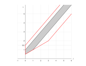
(a) $d=2$: grey region for [4] and new region enclosed by red lines.

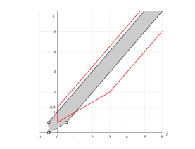
(b) $d=3$: grey region for [3] and new region enclosed by red lines.

Figure 1: Region of regularity $(s,l)$.

2 Notations and normal form

This section is devoted to introducing some basic preparations. We use $S(t)$ and $W_{\alpha}(t)$ to respectively denote Schrödinger and wave semigroup:

$$S(t)\phi=\mathcal{F}^{-1}e^{it\left|\xi\right|^{2}}\hat{\phi},\quad W_{\alpha}(t)\phi=\mathcal{F}^{-1}e^{i\alpha t|\xi|}\hat{\phi},\quad\hat{\phi}=\mathcal{F}\phi,$$ (2.1)

where $\mathcal{F}$ denotes the spatial Fourier transform. Let $\eta_{0}:\mathbb{R}^{d}\rightarrow[0,1]$ denote a radial, smooth function supported in $\{|\xi|\leq 8/5\}$, which is equal to 1 in $\{|\xi|\leq 5/4\}.$ For $k\in\mathbb{Z}$, let $\chi_{k}(\xi)=\eta_{0}\left(\xi/2^{k}\right)-\eta_{0}\left(\xi/2^{k-1}\right)$ and $\chi_{\leq k}(\xi)=\eta_{0}\left(\xi/2^{k}\right).$ Let $P_{k}$, $P_{\leq k}$ denote the operators on $L^{2}\left(\mathbb{R}^{d}\right)$ which are defined by $\widehat{P_{k}u}(\xi)=\chi_{k}(|\xi|)\widehat{u}(\xi)$, $\widehat{P_{\leq k}u}(\xi)=\chi_{\leq k}(|\xi|)\widehat{u}(\xi)$.

Let $s,l\in\mathbb{R}$ and $1\leq p,q\leq\infty$. The standard homogeneous Besov and the inhomogeneous Besov spaces are defined respectively by

$$\|f\|_{\dot{B}_{p,q}^{s}}=\left\|2^{ks}\left\|P_{k}f\right\|_{p}\right\|_{\ell_{k}^{q}(\mathbb{Z})},\ \|f\|_{B_{p,q}^{s}}=\|P_{\leq 0}f\|_{p}+\left(\sum_{k=1}^{\infty}2^{ksq}\left\|P_{k}f\right\|_{p}^{q}\right)^{1/q}.$$ (2.2)

Here, we simply write $B_{p}^{s}=B_{p,2}^{s}$, $H^{s}=B_{2}^{s}$ and the same abbreviations are defined in the homogeneous Besov spaces.

Next, we turn to introduce the normal form reduction. For two functions $N$, $u$ and a fixed $K\in\mathbb{N},K\geq 5$, $Nu$ is divided into

$$Nu=(Nu)_{HH}+(Nu)_{LH}+(Nu)_{HL}.$$ (2.3)

Here $(Nu)_{HH}$ and $(Nu)_{LH}$ are respectively denoted as:

$$(Nu)_{HH}:=\sum_{k_{1},k_{2}\in\mathbb{Z}\atop\left|k_{1}-k_{2}\right|\leq K-1}P_{k_{1}}NP_{k_{2}}u,\ (Nu)_{LH}:=\sum_{k\in\mathbb{Z}}P_{\leq k-K}NP_{k}u,$$

and

$$(Nu)_{HL}:=\sum_{k\in\mathbb{Z}}P_{k}NP_{\leq k-K}u.$$

Denote $\beta\geq K+|\log_{2}\alpha|$. We also define

$$(Nu)_{\alpha L}:=\sum_{k\in\mathbb{Z}\atop k\leq\beta}P_{k}NP_{\leq k-K}u,\ (Nu)_{L\alpha}:=(uN)_{\alpha L},$$ (2.4)

$$(Nu)_{XL}:=\sum_{k\in\mathbb{Z}\atop k>\beta}P_{k}NP_{\leq k-K}u,\ (Nu)_{LX}:=(uN)_{XL},$$

so that

$$(Nu)_{HL}=(Nu)_{\alpha L}+(Nu)_{XL}.$$ (2.5)

For any such index $*=HH,HL,\alpha L,$ etc., the bilinear multiplier is denoted by

$$\mathcal{F}(Nu)_{*}=\int\mathcal{P}_{*}\hat{N}(\xi-\eta)\hat{u}(\eta)d\eta.$$ (2.6)

In view of Duhamel’s formula and the normal form reduction as in [1] and [10], the system $\eqref{equivalent1.1}$ can be rewritten as the following integral equations:

$$u= S(t)u_{0}-S(t)\Omega(N,u)(0)+\Omega(N,u)(t)$$ (2.7)

$$-i\int_{0}^{t}S(t-s)(Nu)_{LH+HH+\alpha L}(s)ds$$

$$-i\int_{0}^{t}S(t-s)\Omega\left(\alpha D|u|^{2},u\right)(s)ds-i\int_{0}^{t}S(t-s)\Omega(N,Nu)(s)ds$$

for $\Omega(f,g)=\mathcal{F}^{-1}\int\mathcal{P}_{XL}\frac{\hat{f}(\xi-\eta)\hat{g}(\eta)}{-|\xi|^{2}+\alpha|\xi-\eta|+|\eta|^{2}}d\eta.$

$$N= W_{\alpha}(t)N_{0}-W_{\alpha}(t)D\tilde{\Omega}(u,u)(0)+D\tilde{\Omega}(u,u)(t)$$ (2.8)

$$-i\int_{0}^{t}W_{\alpha}(t-s)\alpha D(u\bar{u})_{HH+\alpha L+L\alpha}(s)ds$$

$$-i\int_{0}^{t}W_{\alpha}(t-s)(D\tilde{\Omega}(Nu,u)+D\tilde{\Omega}(u,Nu))(s)ds$$

for $\tilde{\Omega}(f,g)=\mathcal{F}^{-1}\int\mathcal{P}_{XL+LX}\frac{\alpha\hat{f}(\xi-\eta)\hat{\bar{g}}(\eta)}{|\xi-\eta|^{2}-|\eta|^{2}-\alpha|\xi|}d\eta.$

Therefore, the equations, after normal form reduction, can be read as

$$\begin{array}[]{l}\left(i\partial_{t}+D^{2}\right)(u-\Omega(N,u))=(Nu)_{LH+HH+\alpha L}+\Omega\left(\alpha D|u|^{2},u\right)+\Omega(N,Nu),\\ \left(i\partial_{t}+\alpha D\right)(N-D\tilde{\Omega}(u,u))=\alpha D|u|_{HH+\alpha L+L\alpha}^{2}+D\tilde{\Omega}(Nu,u)+D\tilde{\Omega}(u,Nu).\end{array}$$ (2.9)

We will use the following Strichartz estimates for the Schrödinger and the wave equation.

Lemma 2.1

(Strichartz estimates, see [14]) For any functions $\phi(x)$ and $f(t,x)$,

(1) if $(q,r)$ and $(\tilde{q},\tilde{r})$ both satisfy the Schrödinger-admissible condition:

$$2\leq q,r\leq\infty,\frac{1}{q}=\frac{d}{2}\left(\frac{1}{2}-\frac{1}{r}\right),(q,r,d)\neq(2,\infty,2),$$ (2.10)

where

$$\begin{cases}2\leq r<\infty,&d=2,\\ 2\leq r\leq 6,&d=3,\end{cases}$$ (2.11)

then

$$\|S(t)\phi\|_{L_{t}^{\infty}H_{x}^{s}\cap L_{t}^{q}B_{r}^{s}}\lesssim\|\phi\|_{H^{s}},$$ (2.12)

$$\left\|\int^{t}_{0}S(t-s)f(s)ds\right\|_{L_{t}^{\infty}H_{x}^{s}\cap L_{t}^{q}B_{r}^{s}}\lesssim\left\|f\right\|_{L^{\tilde{q}^{\prime}}_{t}B^{s}_{\tilde{r}^{\prime}}}.$$ (2.13)

(2) If $(\tilde{q},\tilde{r})$ satisfies the wave-admissible condition:

$$2\leq\tilde{q},\tilde{r}\leq\infty,\frac{1}{\tilde{q}}=\frac{d-1}{2}\left(\frac{1}{2}-\frac{1}{\tilde{r}}\right),(\tilde{q},\tilde{r},d)\neq(2,\infty,3),$$ (2.14)

where

$$\begin{cases}2\leq\tilde{r}\leq\infty,&d=2,\\ 2\leq\tilde{r}<\infty,&d=3,\end{cases}$$ (2.15)

then

$$\|W_{\alpha}(t)\phi\|_{L_{t}^{\infty}H_{x}^{l}}\lesssim\|\phi\|_{H^{l}},$$ (2.16)

$$\left\|\int^{t}_{0}W_{\alpha}(t-s)f(s)ds\right\|_{L_{t}^{\infty}H_{x}^{l}}\lesssim\left\|f\right\|_{L^{\tilde{q}^{\prime}}_{t}B^{l}_{\tilde{r}^{\prime}}}.$$ (2.17)

3 Local well-posedness for $d=3$

In this section, we consider the local well-posedness for $d=3$. According to Lemma 2.1, we define the following spaces:

$$u\in X^{s}:= C\left([-T,T];H^{s}\left(\mathbb{R}^{3}\right)\right)\cap L^{\infty}\left([-T,T];H^{s}\left(\mathbb{R}^{3}\right)\right)$$ (3.1)

$$\cap L^{q}\left([-T,T];B^{s}_{\frac{6q}{3q-4}}\left(\mathbb{R}^{3}\right)\right),$$

and

$$N\in Y^{l}:=C\left([-T,T];H^{l}\left(\mathbb{R}^{3}\right)\right)\cap L^{\infty}\left([-T,T];H^{l}\left(\mathbb{R}^{3}\right)\right),$$ (3.2)

for $2<q\leq\infty$ and $T>0$. Finally, we determine $q=8/3$, and so (3.1) is rewritten as

$$u\in X^{s}:= C\left([-T,T];H^{s}\left(\mathbb{R}^{3}\right)\right)\cap L^{\infty}\left([-T,T];H^{s}\left(\mathbb{R}^{3}\right)\right)$$ (3.3)

$$\cap L^{8/3}\left([-T,T];B^{s}_{4}\left(\mathbb{R}^{3}\right)\right).$$

The $q$ selection will be shown in the following subsections.

We now turn to prove multilinear estimates for the nonlinear terms of $\eqref{final equation}$ in the above spaces. For brevity, we selectively keep some dependence of the constants on $(s,l)$ and $\beta$.

3.1 Quadratic terms

Since we use the contraction mapping principle, $u$ and $N$ must have closed $X^{s}$ and $Y^{l}$ estimates, respectively. In terms of Hölder’s inequality for quadratic terms, we apply the following Strichartz estimates:

$$\left\|\int^{t}_{0}S(t-s)(Nu)_{LH+HH+\alpha L}(s)ds\right\|_{L_{t}^{\infty}H^{s}\cap L_{t}^{8/3}B^{s}_{4}}\lesssim\left\|(Nu)_{LH+HH+\alpha L}\right\|_{L^{8/5}_{t}B^{s}_{4/3}},$$ (3.4)

and

$$\left\|\int_{0}^{t}W_{\alpha}(t-s)D(uv)_{HH+\alpha L+L\alpha}(s)ds\right\|_{L_{t}^{\infty}H^{l}}\lesssim\left\|D(uv)_{HH+\alpha L+L\alpha}\right\|_{L_{t}^{4/3}B^{l}_{4/3}}.$$ (3.5)

In addition, admissible conditions yield that the range of $q$ in (3.1) should be $2<q<4$ if we directly substitute spaces (3.1) and (3.2) into (3.4) and (3.5), respectively.

Lemma 3.1

(1) If $s,l\geq 0$, then for any $N(x)$ and $u(x)$,

$$\left\|(Nu)_{LH+HH}\right\|_{L^{8/5}_{t}B^{s}_{4/3}}\lesssim T^{1/4}\|N\|_{L_{t}^{\infty}H^{l}}\|u\|_{L_{t}^{8/3}B_{4}^{s}}.$$ (3.6)

$$\left\|(Nu)_{\alpha L}\right\|_{L^{8/5}_{t}B^{s}_{4/3}}\lesssim T^{1/4}C(\beta)\|N\|_{L_{t}^{\infty}H^{l}}\|u\|_{L_{t}^{q}B_{4}^{s}}.$$ (3.7)

(2) If $2s\geq l+1$, then for any $u(x)$ and $v(x)$,

$$\left\|D(uv)_{HH}\right\|_{L_{t}^{4/3}B^{l}_{4/3}}\lesssim T^{3/8}\|u\|_{L^{\infty}_{t}H^{s}}\|v\|_{L^{8/3}_{t}B_{4}^{s}}.$$ (3.8)

$$\left\|D(uv)_{\alpha L+L\alpha}\right\|_{L_{t}^{4/3}B^{l}_{4/3}}\lesssim T^{3/8}C(\beta)\|u\|_{L^{\infty}_{t}H^{s}}\|v\|_{L^{8/3}_{t}B_{4}^{s}}.$$ (3.9)

Proof 1

For (1), we begin with the $(Nu)_{LH}$ part. Clearly, the norm for $t$ follows directly from Hölder’s inequality. By $(Nu)_{LH}=\sum_{j\in\mathbb{Z}}P_{\leq j-K}NP_{j}u$ and analyzing the support deduce that

$$\left\|P_{k}(Nu)_{LH}\right\|_{L^{4/3}}\lesssim\sum_{j=k-2}^{k+2}\left\|\left(P_{\leq j-K}N\right)\left(P_{j}u\right)\right\|_{L^{4/3}}\lesssim\sum_{j=k-2}^{k+2}\|N\|_{L^{2}}\left\|P_{j}u\right\|_{L^{4}},$$ (3.10)

then we obtain

$$\left\|(Nu)_{LH}\right\|_{B_{4/3}^{s}}\lesssim\left\|2^{ks}\sum_{j=k-2}^{k+2}\|N\|_{L^{2}}\left\|P_{j}u\right\|_{L^{4}}\right\|_{\ell^{2}_{k}}\lesssim\left\|N\right\|_{H^{l}}\left\|u\right\|_{B^{s}_{4}},$$ (3.11)

where $H^{l}\left(\mathbb{R}^{3}\right)\subset L^{2}\left(\mathbb{R}^{3}\right)$ for $l\geq 0.$

Similarly, the estimate $\left\|(Nu)_{HH}\right\|_{L_{t}^{8/5}B_{4/3}^{s}}\lesssim T^{1/4}\|N\|_{L_{t}^{\infty}H^{l}}\|u\|_{L_{t}^{8/3}B_{4}^{s}}$ is a straightforward result as the proof given in $\eqref{LH}$.

In particular, concerning the fact that $(Nu)_{\alpha L}$ is in the support of $k\sim j\lesssim\beta$, we can conclude

$$\left\|(Nu)_{\alpha L}\right\|_{L_{t}^{8/5}B^{s}_{4/3}}\lesssim T^{1/4}2^{2\beta s}\left\|N\right\|_{L_{t}^{\infty}H^{l}}\left\|u\right\|_{L_{t}^{8/3}B^{s}_{4}},$$ (3.12)

where we require $l\geq 0$ and $s\geq 0.$ Thus, (1) of Lemma 3.1 is proven.

The proof for (2) follows in a similar manner.

Remark 3.1

In view of the admissible conditions in Lemma 2.1, we can verify that for the proof of (1), the norm of $u$ can only adopt the space $L^{8/3}_{t}B_{4}^{s}$, instead of $L_{t}^{\infty}H^{s}$. The same verification is true for the space selections in the proof for (2).

3.2 Boundary terms

We now turn to the boundary terms estimates. However, prior to that, we will review the crucial formulas given in [1]. Take $\Omega(N,u)$ as an example. By Coifman Meyer type bilinear multiplier and Bernstein estimates, we obtain

$$\left\|P_{k}\langle D\rangle D\Omega(N,u)\right\|_{L^{p}}\lesssim\sum_{k_{0}=k-2}^{k+2}\left\|P_{k_{0}}N\right\|_{L^{p_{1}}}\sum_{k_{1}\leq k_{0}-K\atop k_{0}>\beta}\left\|P_{k_{1}}u\right\|_{L^{p_{2}}}$$ (3.13)

$$\lesssim\sum_{k_{0}=k-2}^{k+2}2^{k_{0}^{+}\left(\frac{3}{q_{1}}-\frac{3}{p_{1}}-l\right)}\left\|P_{k_{0}}N\right\|_{B^{l}_{q_{1}}}\sum_{k_{1}\leq k_{0}-K\atop k_{0}>\beta}2^{k_{1}\left(\frac{3}{q_{2}}-\frac{3}{p_{2}}\right)-k_{1}^{+}s}\left\|P_{k_{1}}u\right\|_{B_{q_{2}}^{s}}$$

with

$$\left\{\begin{array}[]{l}k,k_{0},k_{1}\in\mathbb{Z},\\ p,p_{1},p_{2},q_{1},q_{2}\in[1,\infty],\\ 1/p=1/p_{1}+1/p_{2},\\ p_{1}\geq q_{1},p_{2}\geq q_{2},\end{array}\right.$$ (3.14)

where $k_{i}^{+}:=\max(k_{i},0)$, using $P_{\leq 0}B_{p}^{s}\subset\dot{B}_{p,\infty}^{0}$ for the lower frequency component. The same estimate also holds for the bilinear operator $\tilde{\Omega}$.

Lemma 3.2

For any $\theta_{i}(s,l)\geq 0$, as well as functions $N(x)$, $u(x)$, and $v(x)$, we have the following:

(1) If $l\geq-1/2$, $s\leq l+2$ and $(s,l)\neq\left(3/2,-1/2\right)$, then

$$\|\Omega(N,u)\|_{L_{t}^{\infty}H^{s}}\lesssim 2^{-\beta\theta_{1}}\|N\|_{L_{t}^{\infty}H^{l}}\|u\|_{L_{t}^{\infty}H^{s}}.$$ (3.15)

(2) If $l\geq-1/2$, $s\leq l+5/4$ and $(s,l)\neq\left(3/4,-1/2\right)$, then

$$\|\Omega(N,u)\|_{L_{t}^{8/3}B^{s}_{4}}\lesssim 2^{-\beta\theta_{2}}\|N\|_{L_{t}^{\infty}H^{l}}\|u\|_{L_{t}^{8/3}B^{s}_{4}}.$$ (3.16)

(3) If $s\geq\text{max}\left\{l-1,l/2+1/4\right\}$ and $(s,l)\neq\left(3/2,5/2\right)$, then

$$\|D\tilde{\Omega}(u,v)\|_{L_{t}^{\infty}H^{l}}\lesssim 2^{-\beta\theta_{3}}\|u\|_{L_{t}^{\infty}H^{s}}\|v\|_{L_{t}^{\infty}H^{s}}.$$ (3.17)

Proof 2

Here we prove $\eqref{boundary2}$ as an example. In view of $\eqref{crucial}$, a short computation with $(p,p_{1},p_{2},q_{1},q_{2})=\left(4,4,\infty,2,4\right)$ shows that

$$\left\|\Omega(N,u)\right\|_{B^{s}_{4}} \lesssim\left\|2^{k^{+}\left(s-l-5/4\right)}\left\|P_{k}N\right\|_{H^{l}}\sum\limits_{k_{1}\leq k-K\atop k>\beta}2^{3k_{1}/4-k_{1}^{+}s}\left\|P_{k_{1}}u\right\|_{B^{s}_{4}}\right\|_{\ell^{2}_{k}}.$$ (3.18)

It suffices to discuss

$$2^{k^{+}\left(s-l-5/4\right)}\sum\limits_{k_{1}\leq k-K\atop k>\beta}2^{3k_{1}/4-k_{1}^{+}s}.$$ (3.19)

First, the summation over $k_{1}\leq k-K$ deduces

$$k_{1}\leq 0\Rightarrow\sum\limits_{k_{1}\leq k-K}2^{3k_{1}/4-k_{1}^{+}s}\lesssim 1,$$ (3.20)

and

$$0<k_{1}\leq k-K\Rightarrow\sum\limits_{k_{1}\leq k-K}2^{3k_{1}/4-k_{1}^{+}s}\left\{\begin{array}[]{ll}k,&s=3/4,\\ 1,&s>3/4,\\ 2^{k\left(3/4-s\right)},&s<3/4.\end{array}\right.$$ (3.21)

Then, by a summation over $k$, we obtain for $\theta_{2}(s,l)\geq 0$, $\eqref{summation}\lesssim 2^{-\beta\theta_{2}(s,l)}$ if $l\geq-1/2$, $s\leq l+5/4$ and $(s,l)\neq\left(3/4,-1/2\right)$. This and $\left\|P_{k}N\right\|_{H^{l}}\in\ell_{k}^{2}$, together with Hölder’s inequality for $t$ lead to (3.16).

Since the proofs are all similar, we only give the choices of $(p,p_{1},p_{2},q_{1},q_{2})$ for (3.15) and (3.17), both of which are $\left(2,2,\infty,2,2\right)$.

Remark 3.2

(1) We now explain how to determine $p,p_{1},p_{2},q_{1},q_{2}$ for $\eqref{boundary2}$. In order to guarantee that $u$ and $N$, here mainly corresponding to $t$, respectively have closed $X^{s}$ and $Y^{l}$ estimates when using Hölder’s inequality, we shall be forced to take $q_{1}=2$, and $q_{2}=4.$ In terms of the confined conditions in $\eqref{crucial condition}$, $p_{1}$ should be $\max\{p,q_{1}\}=4$. Furthermore, $1/p=1/p_{1}+1/p_{2}$ derives $p_{2}=\infty$. The same method of parameter selection also holds for (3.15) and (3.17).

(2) The range of $q$ here should be $2<q\leq\infty$ if spaces (3.1) and (3.2) are directly used for discussion.

3.3 Cubic terms

In this section, we deal with the cubic terms.

Lemma 3.3

For any $M(x),N(x),u(x),v(x)$, we have the following:

(1) If $l\geq-1/4$, $s\leq\min\{l+2,2l+5/4\}$ and $(s,l)\neq\left(7/4,-1/4\right),\left(11/4,3/4\right),\\ \left(3/4,-1/4\right)$, then

$$\|\Omega(M,Nu)\|_{L^{8/5}_{t}B_{4/3}^{s}}\lesssim T^{1/4}\|M\|_{L^{\infty}_{t}H^{l}}\|N\|_{L^{\infty}_{t}H^{l}}\|u\|_{L^{8/3}_{t}B_{4}^{s}}.$$ (3.22)

(2) If $s\geq 1/2,$ then

$$\|\Omega(D(uv),w)\|_{L^{8/5}_{t}B_{4/3}^{s}}\lesssim T^{1/4}\left\|\|u\|_{H^{s}}\|v\|_{B_{4}^{s}}+\|u\|_{B_{4}^{s}}\|v\|_{H^{s}}\right\|_{L_{t}^{8/3}}\|w\|_{L_{t}^{\infty}H^{s}}.$$ (3.23)

(3) If $s\geq 1/4$, $l\leq\min\{s+1,2s+1/4\}$ and $(s,l)\neq\left(1/4,3/4\right),\left(3/4,7/4\right)$, then

$$\|D\tilde{\Omega}(Nu,v)\|_{L^{1}_{t}H^{l}}+\|D\tilde{\Omega}(v,Nu)\|_{L^{1}_{t}H^{l}}$$ (3.24)

$$\lesssim T^{1/4}\|N\|_{L^{\infty}_{t}H^{l}}\|u\|_{L^{8/3}_{t}B_{4}^{s}}\|v\|_{L^{8/3}_{t}B_{4}^{s}}.$$

Proof 3

It suffices to prove (1) as an example. We obtain the following from $\eqref{crucial}$:

$$\left\|\Omega(M,Nu)\right\|_{B^{s}_{4/3}} \lesssim\left\|2^{k(s-2)}\left\|P_{k}M\right\|_{L^{p_{1}}}\sum_{k_{1}\leq k-K\atop k>\beta}\left\|P_{k_{1}}(Nu)\right\|_{L^{\sigma}}\right\|_{\ell_{k}^{2}}.$$ (3.25)

Furthermore, we obtain three cases:

$$\left\|P_{k_{1}}(Nu)\right\|_{L^{\sigma}}\lesssim \sum_{k_{2}=k_{1}-2}^{k_{1}+2}\left\|P_{k_{2}}u\right\|_{L^{p_{2}}}\sum_{k_{3}\leq k_{2}-K}\left\|P_{k_{3}}N\right\|_{L^{p_{3}}}$$ Case1

$$+\sum_{k_{2}=k_{1}-2}^{k_{1}+2}\left\|P_{k_{2}}u\right\|_{L^{p_{2}}}\sum_{|k_{3}-k_{2}|\leq K-1}\left\|P_{k_{3}}N\right\|_{L^{p_{3}}}$$ Case2

$$+\sum_{k_{3}=k_{1}-2}^{k_{1}+2}\left\|P_{k_{3}}N\right\|_{L^{p_{3}}}\sum_{k_{2}\leq k_{3}-K}\left\|P_{k_{2}}u\right\|_{L^{p_{2}}},$$ Case3

where

$$\left\{\begin{array}[]{l}k,k_{i}\ \in\mathbb{Z},\\ p_{i},q_{i}\in[1,\infty],\\ 3/4=1/p_{1}+1/\sigma,1/\sigma=1/p_{2}+1/p_{3},\\ p_{i}\geq q_{i}.\end{array}\right.$$ (3.26)

Case 1: For $k_{3}\lesssim k_{2}\sim k_{1}\lesssim k$, concerning (3.13), we have

$$2^{ks}\left\|P_{k}\Omega(M,Nu)\right\|_{L^{p}(\text{case 1})}$$ (3.27)

$$\lesssim 2^{k^{+}\left(s-2+\frac{3}{q_{1}}-\frac{3}{p_{1}}-l\right)}\sum_{k_{1}\lesssim k}2^{k_{1}\left(\frac{3}{q_{2}}-\frac{3}{p_{2}}\right)-k_{1}^{+}s}\sum_{k_{3}\lesssim k_{1}}2^{k_{3}\left(\frac{3}{q_{3}}-\frac{3}{p_{3}}\right)-k_{3}^{+}l}$$

$$\quad\times\left\|P_{k}M\right\|_{B^{l}_{q_{1}}}\left\|P_{k_{1}}u\right\|_{B^{s}_{q_{2}}}\left\|P_{k_{3}}N\right\|_{B_{q_{3}}^{l}}.$$

First considering $\left(k_{1}>0,k_{3}>0\right)$, we obtain

$$\eqref{case11}\lesssim 2^{k\left(s-2-l\right)}\sum_{k_{1}\lesssim k}2^{-k_{1}s}\sum_{k_{3}\lesssim k_{1}}2^{k_{3}\left(3/2-l\right)}\left\|P_{k}M\right\|_{H^{l}}\left\|P_{k_{1}}u\right\|_{B^{s}_{4}}\left\|P_{k_{3}}N\right\|_{H^{l}}$$ (3.28)

with $(p,\sigma,p_{1},p_{2},p_{3},q_{1},q_{2},q_{3})=\left(4/3,4,2,4,\infty,2,4,2\right)$. The summation over $k_{3}$ and $k_{1}$ deduces

$$l<3/2:\left\{\begin{array}[]{ll}-s+3/2-l>0\Rightarrow 2^{k\left(-1/2-2l\right)},\\ -s+3/2-l<0\Rightarrow 2^{k\left(-l+s-2\right)},\\ -s+3/2-l=0\Rightarrow k2^{k\left(-l+s-2\right)},\end{array}\right.$$ (3.29)

$$l>3/2:\left\{\begin{array}[]{ll}s<0\Rightarrow 2^{k\left(-l-2\right)},\\ s>0\Rightarrow 2^{k\left(-l+s-2\right)},\\ s=0\Rightarrow k2^{k\left(-l+s-2\right)},\end{array}\right.$$ (3.30)

and

$$l=3/2:\left\{\begin{array}[]{ll}s<0\Rightarrow k2^{k\left(-l-2\right)},\\ s>0\Rightarrow 2^{k\left(-l+s-2\right)},\\ s=0\Rightarrow k2^{k\left(-l+s-2\right)}.\end{array}\right.$$ (3.31)

By summation over $k$, we can see $l<3/2$ is fine if $l\geq-1/4$, $s\leq l+2$ and $(s,l)\neq\left(7/4,-1/4\right)$; $l>3/2$ is fine if $s\leq l+2$; and $l=3/2$ is fine if $s\leq l+2$. To sum up, the summation of (3.28) is bounded provided that $l\geq-1/4$, $s\leq l+2$ and $(s,l)\neq\left(7/4,-1/4\right)$.

For $\left(k_{1}>0,k_{3}\leq 0\right)$ and $\left(k_{1}\leq 0\right)$ meanwhile, it is clear that the boundedness results can be contained by $\left(k_{3}>0,k_{1}>0\right)$. The same discussion is true for $\bf{Case2}$ and $\bf{Case3}$, hence we will omit part of proof.

Case 2: For $k_{3}\sim k_{2}\sim k_{1}\lesssim k$. As in Case 1, we choose

$$(p,\sigma,p_{1},p_{2},p_{3},q_{1},q_{2},q_{3})=\left(4/3,4,2,4,\infty,2,4,2\right).$$

Differently however, it suffices to discuss $2^{k\left(s-2-l\right)}\sum_{k_{1}\lesssim k}2^{k_{1}\left(-s+3/2-l\right)}$ $\left(k_{1}>0\right)$, which is bounded by

$$\left\{\begin{array}[]{ll}-s+3/2-l>0\Rightarrow 2^{k\left(-1/2-2l\right)},\\ -s+3/2-l<0\Rightarrow 2^{k\left(-l+s-2\right)},\\ -s+3/2-l=0\Rightarrow k2^{k\left(-l+s-2\right)},\end{array}\right.$$ (3.32)

provided that $l\geq-1/4$, $s\leq l+2$ and $(s,l)\neq\left(7/4,-1/4\right)$.

Case 3: For $k_{2}\lesssim k_{3}\sim k_{1}\lesssim k$, the boundedness is relevant to

$$2^{ks}\left\|P_{k}\Omega(M,Nu)\right\|_{L^{p}(\text{case 3})}$$ (3.33)

$$\lesssim 2^{k^{+}\left(s-2+\frac{3}{q_{1}}-\frac{3}{p_{1}}-l\right)}\sum_{k_{1}\lesssim k}2^{k_{1}\left(\frac{3}{q_{3}}-\frac{3}{p_{3}}\right)-k_{1}^{+}l}\sum_{k_{2}\lesssim k_{1}}2^{k_{2}\left(\frac{3}{q_{2}}-\frac{3}{p_{2}}\right)-k_{2}^{+}s}$$

$$\quad\times\left\|P_{k}M\right\|_{B^{l}_{q_{1}}}\left\|P_{k_{1}}N\right\|_{B^{l}_{q_{3}}}\left\|P_{k_{2}}u\right\|_{B_{q_{2}}^{s}}.$$

By summation over $(k_{1}>0,k_{2}>0)$, we obtain with $(p,\sigma,p_{1},p_{2},p_{3},q_{1},q_{2},q_{3})=\left(4/3,4,2,\infty,4,2,4,2\right)$

$$s<3/4:\left\{\begin{array}[]{ll}-s+3/2-l>0\Rightarrow 2^{k\left(-1/2-2l\right)},\\ -s+3/2-l<0\Rightarrow 2^{k\left(s-2-l\right)},\\ -s+3/2-l=0\Rightarrow k2^{k\left(s-2-l\right)},\end{array}\right.$$ (3.34)

$$s>3/4:\left\{\begin{array}[]{ll}3/4-l>0\Rightarrow 2^{k\left(-5/4-2l+s\right)},\\ 3/4-l<0\Rightarrow 2^{k\left(s-2-l\right)},\\ 3/4-l=0\Rightarrow k2^{k\left(s-2-l\right)},\end{array}\right.$$ (3.35)

and

$$s=3/4:\left\{\begin{array}[]{ll}3/4-l>0\Rightarrow k2^{k\left(-5/4-2l+s\right)},\\ 3/4-l<0\Rightarrow 2^{k\left(s-2-l\right)},\\ 3/4-l=0\Rightarrow k2^{k\left(s-2-l\right)}.\end{array}\right.$$ (3.36)

By summation over $k$, $s<3/4$ is fine if $l\geq-1/4,s\leq l+2$ and $(s,l)\neq\left(7/4,-1/4\right)$; $s>3/4$ is fine if $s\leq\min\{l+2,2l+5/4\}$ and $(s,l)\neq\left(11/4,3/4\right)$; and $s=3/4$ is fine if $l\geq-1/4$ and $(s,l)\neq\left(3/4,-1/4\right)$.

Ultimately, an application of Hölder’s inequality for $t$, Case 1, Case 2 and Case 3 together with $\left\|P_{k}M\right\|_{H^{l}}\in\ell_{k}^{2}$ lead to $\eqref{boundary2}$.

The proofs for (2) and (3) are similarly obtained.

Remark 3.3

(1) Concerning Case 1 in the proof for (3.22), we explain how to choose $p,p_{i},q_{i}$. The choices, all based on the confined conditions in $\eqref{crucial condition2}$, are to obtain a wider range of $(s,l)$.

Step 1: We first determine $p$. In terms of (3.27), it is optimal the differences $\frac{1}{q_{1}}-\frac{1}{p_{1}}\geq 0$, $\frac{1}{q_{2}}-\frac{1}{p_{2}}\geq 0$ and $\frac{1}{q_{3}}-\frac{1}{p_{3}}\geq 0$ are all as small as possible, with 0 being the best. On one hand, $p_{1}$, $p_{2}$ and $p_{3}$ should be as small as possible, which means $p$ should be small with $\frac{1}{p}=\frac{1}{p_{1}}+\frac{1}{p_{2}}+\frac{1}{p_{3}}$. In addition, as $p$ comes from the Schrödinger Strichartz estimates in Lemma 2.1, together with the space $\eqref{Xs}$, it is optimal to choose $p=\frac{6q}{3q+4}$.

On the other hand, $q_{1}$, $q_{2}$ and $q_{3}$ should all be as large as possible. Thus, in view of $\eqref{Xs}$ and $\eqref{Yl}$, we observe $q_{1}=2$, $q_{2}=\frac{6q}{3q-4}$ and $q_{3}=2$.

Step 2: Since $k$ is dominant in the summation of the first dyadic decomposition, we have to choose $p_{1}$ preferentially. The condition that $p_{1}$ should be as small as possible, together with $p_{1}\geq\max\{q_{1},p\}$ is briefly described as $p_{1}=\max\{q_{1},p\}$; that is to say $p_{1}=2$. At this time, $\frac{1}{p}=\frac{1}{p_{1}}+\frac{1}{\sigma}$ derives $\sigma=\frac{3q}{2}$.

Step 3: Similar to the above Step 2, $k_{2}$ is dominant in the summation of the second dyadic decomposition. Hence $p_{2}=\max\{q_{2},\sigma\}=\frac{6q}{3q-4}$, where $\frac{6q}{3q-4}\geq\frac{3q}{2}$ deduces that the range of $q$ is $2<q\leq\frac{8}{3}$.

Step 4: Now $p_{3}=\frac{6q}{8-3q}$ by $\frac{1}{\sigma}=\frac{1}{p_{2}}+\frac{1}{p_{3}}$, and we have $p_{3}\geq\max\{q_{3},\sigma\}$.

Step 5: This is a test process. Steps 1 to 4 are just related to the spatial variable in theory. However, considering the spaces $\eqref{Xs}$, $\eqref{Yl}$ and $2<q\leq\frac{8}{3}$, it is imperative to check whether the norms of $u,N,M$ for the time variable $t$ are still reasonable when using Hölder’s inequalities. If not, adjustments must be made for $p,p_{i},q_{i}$. For instance, the parameter selection for proving (3.23) is like this, leaving it to the reader.

Thus, we choose $(p,\sigma,p_{1},p_{2},p_{3},q_{1},q_{2},q_{3})=\left(\frac{6q}{3q+4},\frac{3q}{2},2,\frac{6q}{3q-4},\frac{6q}{8-3q},2,\frac{6q}{3q-4},2\right)$ in Case 1.

(2) Differently to Case 1 and Case 2, $k_{3}$ is dominant in the summation of the second dyadic decomposition in Case 3. That is why we will first choose $p_{3}=\max\{q_{3},\sigma\}=\frac{3q}{2}$ for $2<q\leq\frac{8}{3}$ in Step 3.

3.4 Proof of Theorem 1.2

It is time to prove Theorem 1.2 by applying the multilinear estimates above. For any initial data $\left(u_{0},N_{0}\right)\in H^{s}\left(\mathbb{R}^{3}\right)\times H^{l}\left(\mathbb{R}^{3}\right)$, we define a mapping of $(u,N)\mapsto\Phi_{u_{0},N_{0}}(u,N)=(F(u,N),G(u,N))$, where $F(u,N)$ and $G(u,N)$ are the right-hand sides of equations $\eqref{u}$ and $\eqref{N}$, respectively. Now, the proof proceeds by a standard contraction mapping principle. First, the intersection of ranges for $q$ yields that $q=8/3$ is the optimal choice. In addition, the resolution space is denoted as

$$X(T)=\left\{(u,N):\left\|(u,N)\right\|_{X(T)}\leq\eta=5/2\left(\left\|u_{0}\right\|_{H^{s}}+\left\|N_{0}\right\|_{H^{l}}\right)\right\},$$ (3.37)

where the $X(T)$-norm is given by

$$\left\|(u,N)\right\|_{X(T)}=\left\|u\right\|_{X^{s}}+\left\|N\right\|_{Y^{l}}.$$

By the previous lemmas, we have

$$\left\|F(u,N)\right\|_{X^{s}}$$ (3.38)

$$\lesssim\left\|u_{0}\right\|_{H^{s}}+2^{-\beta\theta_{1}}\left\|N_{0}\right\|_{H^{l}}\left\|u_{0}\right\|_{H^{s}}+2^{-\beta(\theta_{1}+\theta_{2})}\left\|N\right\|_{Y^{l}}\left\|u\right\|_{X^{s}}$$

$$\quad+T^{1/4}(C(\beta)+1)\left\|N\right\|_{Y^{l}}\left\|u\right\|_{X^{s}}+T^{1/4}\left\|u\right\|^{3}_{X^{s}}+T^{1/4}\left\|N\right\|^{2}_{Y^{l}}\left\|u\right\|_{X^{s}},$$

and

$$\left\|G(u,N)\right\|_{Y^{l}} \lesssim\left\|N_{0}\right\|_{H^{l}}+2^{-\beta\theta_{3}}\left\|u_{0}\right\|^{2}_{H^{s}}+2^{-\beta\theta_{3}}\left\|u\right\|^{2}_{X^{s}}$$ (3.39)

$$\quad+T^{3/8}(C(\beta)+1)\left\|u\right\|^{2}_{X^{s}}+T^{1/4}\left\|N\right\|_{Y^{l}}\left\|u\right\|^{2}_{X^{s}}.$$

Without loss of generality, we denote $\theta=\min\left\{\theta_{1},\theta_{3}\right\}$, and $T^{\delta}=\max\left\{T^{1/4},T^{3/8}\right\}$. Hence for any $(u,N),(v,M)\in X(T)$ with the same initial data, it follows that

$$\|\Phi_{u_{0},N_{0}}(u,N)-\Phi_{v_{0},M_{0}}(v,M)\|_{X(T)}$$ (3.40)

$$\leq\left(2^{-\beta\theta}\eta+T^{\delta}(C(\beta)+1)\eta+T^{\delta}C\eta^{2}\right)\left(\|u-v\|_{X^{s}}+\|N-M\|_{Y^{l}}\right).$$

We let $\beta=\beta(\eta)$ satisfy $2^{-\beta\theta}\eta\leq 1/4$ and choose an appropriate $T>0$ such that $T^{\delta}(C(\beta)+1)\eta+T^{\delta}C\eta^{2}\leq 1/4$. Hence we conclude that

$$\|\Phi_{u_{0},N_{0}}(u,N)-\Phi_{v_{0},M_{0}}(v,M)\|_{X(T)}\leq 1/2\left(\|u-v\|_{X^{s}}+\|N-M\|_{Y^{l}}\right).$$ (3.41)

In addition, by denoting $(v,M)=(0,0)$ we get

$$\left\|\Phi_{u_{0},N_{0}}(u,N)\right\|_{X(T)}\leq \eta/2+\left\|u_{0}\right\|_{H^{s}}+\left\|N_{0}\right\|_{H^{l}}+2^{-\beta\theta}\left\|N_{0}\right\|_{H^{l}}\left\|u_{0}\right\|_{H^{s}}$$ (3.42)

$$+2^{-\beta\theta}\left\|u_{0}\right\|^{2}_{H^{s}}\leq\eta.$$

Through this, we can see that $\Phi$ is a contraction mapping for any initial data $(u_{0},N_{0})$. Thus, by the contraction mapping principle , we have a local unique solution in $X^{s}\times Y^{l},$ and the Lipschitz continuity $H^{s}\times H^{l}\rightarrow X^{s}\times Y^{l}$ follows from the standard argument.

4 Local well-posedness for $d=2$

This section is devoted to the case for dimension 2. The spaces here are defined as

$$u\in X^{s}:= C\left([-T,T];H^{s}\left(\mathbb{R}^{2}\right)\right)\cap L^{\infty}\left([-T,T];H^{s}\left(\mathbb{R}^{2}\right)\right)$$ (4.1)

$$\cap L^{q}\left([-T,T];B^{s}_{\frac{2q}{q-2}}\left(\mathbb{R}^{2}\right)\right)$$

for $2<q\leq\infty$, and

$$N\in Y^{l}:=C\left([-T,T];H^{l}\left(\mathbb{R}^{2}\right)\right)\cap L^{\infty}\left([-T,T];H^{l}\left(\mathbb{R}^{2}\right)\right).$$ (4.2)

We ultimately determine $q=4$ for $d=2$. Since the proofs are essentially the same as in the case for dimension 3, we only present the main lemmas.

Lemma 4.1

(Quadratic terms)

(1) If $s,l\geq 0$, then for any $N(x)$ and $u(x)$,

$$\left\|(Nu)_{LH+HH}\right\|_{L_{t}^{4/3}B_{4/3}^{s}}\lesssim T^{1/2}\|N\|_{L_{t}^{\infty}H^{l}}\|u\|_{L_{t}^{4}B_{4}^{s}}.$$ (4.3)

$$\left\|(Nu)_{\alpha L}\right\|_{L_{t}^{4/3}B_{4/3}^{s}}\lesssim T^{1/2}C(\beta)\|N\|_{L_{t}^{\infty}H^{l}}\|u\|_{L_{t}^{4}B_{4}^{s}}.$$ (4.4)

(2) If $2s\geq l+1$, then for any $u(x)$ and $v(x)$,

$$\left\|D(uv)_{HH}\right\|_{L_{t}^{8/7}B^{l}_{4/3}}\lesssim T^{5/8}\|u\|_{L^{\infty}_{t}H^{s}}\|v\|_{L^{4}_{t}B_{4}^{s}}.$$ (4.5)

$$\left\|D(uv)_{\alpha L+L\alpha}\right\|_{L_{t}^{8/7}B^{l}_{4/3}}\lesssim T^{5/8}C(\beta)\|u\|_{L^{\infty}_{t}H^{s}}\|v\|_{L^{4}_{t}B_{4}^{s}}.$$ (4.6)

Lemma 4.2

(Boundary terms) For any $\theta_{i}(s,l)\geq 0$, and functions $N(x),u(x),v(x)$, we have the following:

(1) If $l\geq-1$, $s\leq l+2$ and $(s,l)\neq\left(1,-1\right)$, then

$$\|\Omega(N,u)\|_{L_{t}^{\infty}H^{s}}\lesssim 2^{-\beta\theta_{1}}\|N\|_{L_{t}^{\infty}H^{l}}\|u\|_{L_{t}^{\infty}H^{s}}.$$ (4.7)

(2) If $l\geq-1$, $s\leq l+3/2$ and $(s,l)\neq\left(1/2,-1\right)$, then

$$\|\Omega(N,u)\|_{L_{t}^{4}B^{s}_{4}}\lesssim 2^{-\beta\theta_{2}}\|N\|_{L_{t}^{\infty}H^{l}}\|u\|_{L_{t}^{4}B^{s}_{4}}.$$ (4.8)

(3) If $s\geq\text{max}\left(l-1,l/2\right)$ and $(s,l)\neq(1,2)$, then

$$\|D\tilde{\Omega}(u,v)\|_{L_{t}^{\infty}H^{l}}\lesssim 2^{-\beta\theta_{3}}\|u\|_{L_{t}^{\infty}H^{s}}\|v\|_{L_{t}^{\infty}H^{s}}.$$ (4.9)

Lemma 4.3

(Cubic terms) For any $M(x),N(x),u(x),v(x)$, we have the following:

(1) If $l\geq-1/2,s\leq\min\{l+2,2l+3/2\}$ and $(s,l)\neq\left(3/2,-1/2\right),\left(5/2,1/2\right),\\ \left(1/2,-1/2\right)$, then

$$\|\Omega(M,Nu)\|_{L^{4/3}_{t}B_{4/3}^{s}}\lesssim T^{1/2}\|M\|_{L^{\infty}_{t}H^{l}}\|N\|_{L^{\infty}_{t}H^{l}}\|u\|_{L^{4}_{t}B_{4}^{s}}.$$ (4.10)

(2) If $s\geq-1/4$, then

$$\|\Omega(D(uv),w)\|_{L^{4/3}_{t}B_{4/3}^{s}}\lesssim T^{1/4}\|u\|_{{L_{t}^{4}}B_{4}^{s}}\|v\|_{{L_{t}^{4}}B_{4}^{s}}\|w\|_{L_{t}^{\infty}H^{s}}.$$ (4.11)

(3) If $s\geq 0$, $l\leq\min\{s+1,2s+1/2\}$ and $(s,l)\neq\left(1/2,3/2\right),\left(0,1/2\right)$, then

$$\|D\tilde{\Omega}(Nu,v)\|_{L^{1}_{t}H^{l}}+\|D\tilde{\Omega}(v,Nu)\|_{L^{1}_{t}H^{l}}\lesssim T^{1/2}\|N\|_{L^{\infty}_{t}H^{l}}\|u\|_{L^{4}_{t}B_{4}^{s}}\|v\|_{L^{4}_{t}B_{4}^{s}}.$$ (4.12)

References

- [1] I. Bejenaru, Z. Guo, S. Herr and K. Nakanishi, Well-posedness and scattering for the Zakharov system in four dimensions, Analysis PDE, 8 (2015), no. 8, 2029–2055.
- [2] I. Bejenaru, S. Herr, J. Holmer and D. Tataru, On the 2D Zakharov system with -Schrödinger data, Nonlinearity, 22 (2009), no. 5, 1063–1089.
- [3] I. Bejenaru and S. Herr, Convolutions of singular measures and applications to the Zakharov system, J. Funct. Anal., 261 (2011), no. 2, 478–506.
- [4] J. Bourgain and J. Colliander, On wellposedness of the Zakharov system, Internat. Math. Res. Notices, (1996), no. 11, 515–546.
- [5] T. Candy, S. Herr and K. Nakanishi, The Zakharov system in dimension , preprint, arXiv1912.05820v2.
- [6] J. Colliander, J. Holmer and N. Tzirakis, Low regularity global well-posedness for the Zakharov and Klein-Gordon-Schrödinger systems, Trans. Amer. Math. Soc., 360 (2008), no. 9, 4619–4638.
- [7] D. Fang, H. Pecher and S. Zhong, Low regularity global well-posedness for the two-dimensional Zakharov system, Analysis (Munich), 29 (2009), no. 3, 265–281.
- [8] J. Ginibre, Y. Tsutsumi and G. Velo, On the Cauchy problem for the Zakharov system, J. Funct. Anal., 151 (1997), no. 2, 384–436.
- [9] Z. Guo, S. Lee, K. Nakanishi and C. Wang, Generalized Strichartz estimates and scattering for 3D Zakharov system, Comm. Math. Phys., 331 (2014), no. 1, 239–259.
- [10] Z. Guo and K. Nakanishi, Small energy scattering for the Zakharov system with radial symmetry, Int. Math. Res. Not., (2014), no. 9, 2327–2342.
- [11] Z. Guo and K. Nakanishi, The Zakharov system in 4D radial energy space below the ground state, preprint, arXiv1810.05794.
- [12] Z. Guo, K. Nakanishi and S. Wang, Global dynamics below the ground state energy for the Klein-Gordon-Zakharov system in the 3D radial case, Comm. Partial Differential Equations, 39 (2014), no. 6, 1158–1184.
- [13] I. Kato and K. Tsugawa, Scattering and well-posedness for the Zakharov system at a critical space in four and more spatial dimensions, Differential Integral Equations, 30 (2017), no. 9-10, 763–794.
- [14] M. Keel and T. Tao, Endpoint Strichartz estimates, Amer. J. Math., 120 (1998), no. 5, 955–980.
- [15] N. Kishimoto, Local well-posedness for the Zakharov system on the multidimensional torus, J. Anal. Math., 119 (2013), 213–253.
- [16] H. Pecher, Global solutions with infinite energy for the one-dimensional Zakharov system, Electronic Journal of Differential Equations, 2005 (2005), no. 41, 1–18.
- [17] A. Sanwal, Local well-posedness for the Zakharov system in dimension , preprint, arXiv2103.09259.
- [18] V. E. Zakharov, Collapse of Langmuir waves, Sov. Phys. JETP, 35 (1972), 908–914.