FixNorm: Dissecting Weight Decay for Training Deep Neural Networks

Abstract

Weight decay is a widely used technique for training Deep Neural Networks(DNN). It greatly affects generalization performance but the underlying mechanisms are not fully understood. Recent works show that for layers followed by normalizations, weight decay mainly affects the effective learning rate. However, despite normalizations have been extensively adopted in modern DNNs, layers such as the final fully-connected layer do not satisfy this precondition. For these layers, the effects of weight decay are still unclear. In this paper, we comprehensively investigate the mechanisms of weight decay and find that except for influencing effective learning rate, weight decay has another distinct mechanism that is equally important: affecting generalization performance by controlling cross-boundary risk. These two mechanisms together give a more comprehensive explanation for the effects of weight decay. Based on this discovery, we propose a new training method called FixNorm, which discards weight decay and directly controls the two mechanisms. We also propose a simple yet effective method to tune hyperparameters of FixNorm, which can find near-optimal solutions in a few trials. On ImageNet classification task, training EfficientNet-B0 with FixNorm achieves 77.7%, which outperforms the original baseline by a clear margin. Surprisingly, when scaling MobileNetV2 to the same FLOPS and applying the same tricks with EfficientNet-B0, training with FixNorm achieves 77.4%, which is only 0.3% lower. A series of SOTA results show the importance of well-tuned training procedures, and further verify the effectiveness of our approach. We set up more well-tuned baselines using FixNorm, to facilitate fair comparisons in the community.

1 Introduction

Weight decay is an important trick and has been widely used in training Deep Neural Networks. By constraining the weight magnitude, it is widely believed that weight decay regularizes the model and improve generalization performance(Krizhevsky et al., 2012; Bös, 1996; Bos & Chug, 1996; Krogh & Hertz, 1992). Recently, a series of works Van Laarhoven (2017); Zhang et al. (2018); Hoffer et al. (2018) propose that for layers followed by normalizations, such as BatchNormalization(Ioffe & Szegedy, 2015), the main effect of weight decay is increasing the effective learning rate(ELR). Take the widely adopted Conv-BN block as an example. Since BatchNormalization is scale-invariant, the weight norm of the convolution layer do not actually affect the block’s output, which contradicts the regularization effect of weight decay. On the contrary, the weight norm affects the step size of weight direction, e.g., larger weight norm results in smaller step size. By constraining the weight norm from unlimitedly growing, weight decay is actually increasing the step size of weight direction, thus increasing the ELR.

This interesting discovery arouses our questions: Does it covers the full mechanism(s) of weight decay? If the answer is true, weight decay would be unnecessary since its effect fully overlaps with the original learning rate. Hoffer et al. (2018) shows that the performance can be recovered when training without weight decay by applying an LR correction technique. However, the LR correction coefficient at each step depends on the original training statistics(with weight decay), which makes this technique only a verification of the effective learning rate hypothesis, but can not be used as a practical training method. Moreover, the ELR hypothesis only applies to layers followed by normalizations, and there are layers that do not satisfy this requirement. For example, the final fully-connected layer that commonly used in classification tasks. For these layers, the effects of weight decay are usually omitted (Hoffer et al., 2018), or simply the original weight decay is preserved (Zhang et al., 2018). These problems indicate that the mechanisms of weight decay are still not fully understood.

In this paper we try to investigate the above problems. For the convolution layers that followed by normalizations, we find that simply fixing the overall weight norm to a constant fully recovers the effect of weight decay. For the final fully-connected layer, we find that there is a special effect introduced by weight decay, which influences the generalization performance by controlling the cross-boundary risk. This mechanism is as important as the former investigated ELR, and they together capture most of the effects of weight decay. These two mechanisms are unified into a new training scheme called FixNorm, which discards the weight decay and directly controls the effects of two main mechanisms. By using FixNorm, we fully recover the performance of popular CNNs on large scale classification dataset ImageNet(Deng et al., 2009). Further, we show that the hyperparameters of FixNorm can be easily tuned, and propose a simple yet effective tuning method which only requires a few trials and achieves near-optimal performance. Specifically, by applying tuned FixNorm, we achieve 77.7%(+0.4%) with EfficientNet-B0, 79.5%(+0.3%) with EfficientNet-B1, 73.97%(+1.9%) with MobileNetV2.

Training tricks and network tricks show great impacts on performance, which also introduce difficulties in tuning and bring ambiguities to comparisons. We show that this can be mitigated by using FixNorm. For example, by simply scaling MobileNetV2 to the same FLOPS and applying the same tricks of EfficientNet-B0, training with FixNorm achieves 77.4% top-1 accuracy, while the default training process only get 76.72%. To facilitate fairer comparisons, we apply our FixNorm method to representative CNN architectures and set up new baselines under different settings.

Our contributions can be summarized as follows:

• Except for increasing the effective learning rate, we discover a new mechanism of weight decay which controls the cross-boundary risk, and give a better understanding of weight decay’s effect on generalization performance

• We propose a new training scheme called FixNorm that discards the weight decay and directly controls the effects of two main mechanisms, which not only fully recovers the accuracy of weight decay training, but also makes hyperparameters easier to tune.

• We propose a simple yet effective method to tune hyperparameters of FixNorm and demonstrate efficiency, robustness and SOTA performance on large scale datasets like ImageNet, MS COCO(Lin et al., 2014) and Cityscapes(Cordts et al., 2016)

• By using our approach, we establish well-tuned baselines for popular networks, which we hope can facilitate fairer comparisons in the community

2 Dissecting weight decay for training Deep Neural Networks

2.1 Revisiting the effective learning rate hypothesis

We aim at further understanding the mechanisms of weight decay. Towards this, we first briefly revisit the effective learning rate(ELR) hypothesis. As noted in Hoffer et al. (2018), when BN is applied after a linear layer, the output is invariant to the channel weight vector norm. Denoting a channel weight vector with $\bm{w}$ and $\hat{\bm{w}}=\bm{w}/\|\bm{w}\|_{2}$, channel input as $\bm{x}$, we have

$$\text{BN}(\|\bm{w}\|_{2}\hat{\bm{w}}\bm{x})=\text{BN}(\hat{\bm{w}}\bm{x})$$ (1)

In such case, the gradient is scaled by $1/\|\bm{w}\|_{2}$:

$$\frac{\partial\text{BN}(\|\bm{w}\|_{2}\hat{\bm{w}}\bm{x})}{\partial(\|\bm{w}\|_{2}\hat{\bm{w}})}=\frac{1}{\|\bm{w}\|_{2}}\frac{\partial\text{BN}(\hat{\bm{w}}\bm{x})}{\partial\hat{\bm{w}}}$$ (2)

This scale invariance makes the key feature of the weight vector is its direction. When the weights are updated through stochastic gradient descent at step $t$ and learning rate $\eta$

$$\bm{w}_{t+1}=\bm{w}_{t}-\eta\nabla\bm{L}_{t}(\bm{w}_{t})$$ (3)

As in Hoffer et al. (2018), one can derive that the step size of the weight direction is approximately proportional to

$$\bm{\hat{w}}_{t+1}-\bm{\hat{w}}_{t}\propto\frac{\eta}{\|\bm{w}_{t}\|_{2}^{2}}$$ (4)

Based on this formulation, the ELR hypothesis can be explained as follows: when applying weight decay to layers followed by normalization, it prevents weight norm from unlimitedly growing, which preserves the step size of weight direction, thus “increasing the effective learning rate”

However, this phenomenon is still not fully investigated. Hoffer et al. (2018) propose an LR correction technique that can train DNNs to similar performance without weight decay. However, this LR correction technique needs to mimic the effective step size from training with weight decay. Similar techniques have also been proposed in Zhang et al. (2018). These techniques act as proofs of the ELR hypothesis, but can not be used as practical training methods. On the other hand, as the hypothesis is based on the scale invariance brought by normalizations, there are layers that do not satisfy this precondition. For example, the final fully-connected(FC) layers that commonly used in classification tasks. As experiments in Zhang et al. (2018)(Figure 4), there is a clear gap between whether weight decay is applied to the FC layer. These problems indicate that the mechanisms of weight decay are still not fully understood.

2.2 Discarding weight decay for convolution layers

We first consider discarding weight decay for convolution layers. Since ELR hypothesis indicates that the main effect of weight decay on convolution layers is produced by constraining weight vector norm, we investigate how weight vector norm changes during training. Denoting the weights in all convolution layers as a single verctor $\bm{W}^{\text{Conv}}$, we plot $\|\bm{W}^{\text{Conv}}\|_{2}$ in Fig 1. ResNet50He et al. (2016) is trained on ImageNet for 100 epochs with $lr=0.4$ and weght decay$\lambda=0.0001$. Other settings follow general setups in 3.

Figure 1: Left: $\|\bm{W}^{\text{Conv}}\|_{2}$ of WD training Right: top-1 accuracy for Algo 6 and WD training, both learning rates are found by gridsearch

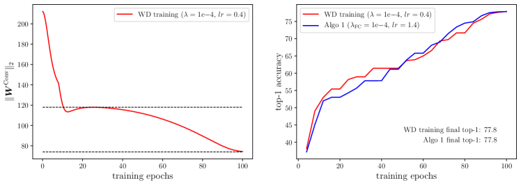
From Fig 1 left, the curve can be divided into two parts. In the first part, $\|\bm{W}^{\text{Conv}}\|_{2}$ decreases rapidly, which will increase the effective learning rate according to the ELR hypothesis. However, we already adopt the learning rate warmup strategy, therefore this part of effect is duplicate and can be discarded. In the second part, which occupies the majority of training, $\|\bm{W}^{\text{Conv}}\|_{2}$ changes slowly in a relatively stable range. From these observations, we propose to fix $\|\bm{W}^{\text{Conv}}\|_{2}$ to a constant, as in Algo 6. We rescale $\bm{W}^{\text{Conv}}$ after each optimization step, which does not change outputs of the network but substantially maintains the effective learning rate. While WD training controls the weight norm dynamically by a hyperparameter $\lambda$, Algo 6 directly fixes the norm to a constant. Since this constant can be any value, we choose it as the $\|\bm{W}^{\text{Conv}}\|_{2}$ at initialization for simplicity.

Algorithm 1 Fixing the weight norm of convolution layers

Input: initial learning rate $lr$, total steps $T$, weight decay on final FC layer $\lambda_{\text{FC}}$, momentum $\mu$, training samples $\bm{x}$, corresponding labels $\bm{y}$
Initialization: velocity $\bm{V}_{0}\leftarrow\bm{0}$, random initialize weight vector $\bm{W_{0}}$

1:for $t$ in 0, …, $T-1$ do

2:     $\bm{x},\bm{y}$ $\leftarrow$ BatchSampler($t$)

3:     $\widehat{\mathcal{L}}_{t}(\bm{W}_{t})\leftarrow\sum\mathcal{L}(f(x;\bm{W}_{t}),y)+\frac{1}{2}\lambda_{\text{FC}}\|\bm{W}_{t}^{\text{FC}}\|_{2}^{2}$

4:     $\bm{V}_{t+1}\leftarrow\mu\bm{V}_{t}+\nabla\widehat{\mathcal{L}}_{t}(\bm{W}_{t})$

5:     $\eta_{t}\leftarrow$ GetLRScheduleMultiplier$(t)$

6:     $\bm{W}_{t+1}\leftarrow\bm{W}_{t}-lr\times\eta_{t}\times\bm{V}_{t+1}$

7:     $\bm{W}^{\text{Conv}}_{t+1}\leftarrow\frac{\bm{W}^{\text{Conv}}_{t+1}}{\|\bm{W}^{\text{Conv}}_{t+1}\|_{2}}\|\bm{W}^{\text{Conv}}_{0}\|_{2}$

8:end for

Since the fixed weight norm in Algo 6 is substantially different from WD training, their optimal learning rates are different as well. To be fair, we grid search the $lr$ for both Algo 6 and WD training and compare the best performance. As shown in Fig 1 right, Algo 6 achieves same top-1 accuracy of WD training. These results demonstrate that for convolution layers followed by BN, weight decay can be discarded. Note that we preserve $\lambda^{\text{FC}}$ for the final FC layer, which will be addressed in the next subsection.

2.3 Effects on final fully-connected layers

As noted in section 2.1, the final FC layer does not satisfy the precondition of the ELR hypothesis. To investigate the effects of weight decay on this layer, we first try to make it scale-invariant. We apply three modifications on Algo 6: (1) replace original FC layer with WN-FC layer; (2) replace $\bm{W}^{\text{Conv}}$ in line 7 of Algo 6 with $\bm{W}^{\text{Conv+FC}}$; (3) set $\lambda^{\text{FC}}=0$. This modified algorithm is denoted as Algo 1@WN-FC. WN-FC layer is normal FC layer applied with weight normalization(Salimans & Kingma, 2016). Original FC and WN-FC layer are formulated as follows:

$$\text{FC}(x;\bm{W}^{\text{FC}}) =x^{\mathsf{T}}\bm{W}^{\text{FC}}$$ (5)

$$\text{WN-FC}(x;\bm{W}^{\text{FC}},g) =\frac{x^{\mathsf{T}}\bm{W}^{\text{FC}}}{\|\bm{W}^{\text{FC}}\|_{2}}\times g$$ (6)

Figure 2: Training ResNet50 on ImageNet with Algo 6, Algo 1@WN-FC and Algo 1@FixNorm-FC. Left: top-1 accuracy Top right: weight norm of the final FC layer ($\|\bm{W}^{\text{FC}}\|_{2}$ for FC, $g$ for WN-FC and FixNorm-FC) Bottom right: MCBR

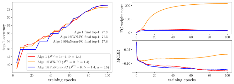
We compare Algo 6 and Algo 1@WN-FC by training ResNet50 on ImageNet. As can be seen in Fig 2 left, there is a clear gap between Algo 6 and Algo 1@WN-FC, which implies that weight decay has additional effects beyond preserving ELR on final FC layers.

Now lets combine equation 6 with softmax cross-entropy loss $\mathcal{L}$, $s_{i}=\frac{x^{\mathsf{T}}\bm{W}_{i}}{\|\bm{W}\|_{2}}g$ denotes the logits value of class $i$, $p_{i}$ denotes the probability of class $i$, $k$ for the label class and $j$ for other classes. We have(for full derivations please refer to supplymentary materials),

$$\mathcal{L}(x,k) =-\log p_{k}=-\log\frac{e^{s_{k}}}{\sum e^{s_{j}}}$$ (7)

$$-\frac{\partial\mathcal{L}(x,k)}{\partial x} =\frac{g}{\|\bm{W}\|_{2}}\sum_{j\neq k}p_{j}(\bm{W}_{k}-\bm{W}_{j})$$ (8)

Figure 3: Ilustration of feature space

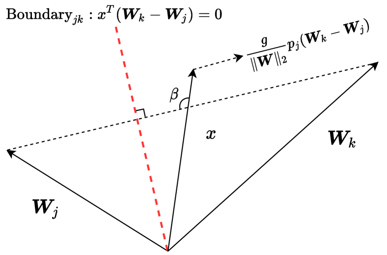
Given $\bm{W}$, the gradient is actually driving $x$ from other class center $\bm{W}_{j}$ towards label class center $\bm{W}_{k}$, where the magnitude depends on $p_{j}$ and $g$. Note that $p_{j}$ also depends on $g$ through the softmax function. When $x$ is correctly classified and $g$ continuously grows, $p_{j}$ will rapidly shrink and weaken the gradient. As illustrated in Fig 3, this will leave $x$ being closer to the class boundary between $\bm{W}_{j}$ and $\bm{W}_{k}$(larger $\cos\beta$), which is less discriminative. This ambiguous feature space is prone to distribution shift between training and testing, therefore may result in poor generalization.

To quantitively verify this explaination, we define Mean Cross-Boundary Risk(MCBR):

$$\text{MCBR}(x,k,\bm{W})=\frac{1}{\#class-1}\sum_{j\neq k}\cos(x,\bm{W}_{j}-\bm{W}_{k})$$ (9)

MCBR shows how much $x$ is lean to the class boundaries, ranging from -1 to 1. The larger MCBR is, the more likely $x$ will cross the class boundaries during testing. We compare the weight norm of FC layer($g$ for WN-FC layer) and MCBR for Algo 6 and Algo 1@WN-FC in Fig 2 top right and bottom right. It can be clearly observed that without constraint, $g$ continuously grows and leads to higher MCBR. This explains why Algo 1@WN-FC generalize poorly.

Based on these analysis, we propose to constrain $g$ from exceeding a given upperbound $\alpha$, denoted as FixNorm-FC. $\sqrt{\#class}$ normalize the upper bound across different number of classes.

$$\text{FixNorm-FC}(x;\bm{W}^{FC},g,\alpha)=\frac{x^{\mathsf{T}}\bm{W}^{FC}}{\|\bm{W}^{FC}\|_{2}}\times\min(g,\alpha*\sqrt{\#class})$$ (10)

Note that $\bm{W}^{FC}$ and $g$ are learnable parameters, while $\alpha$ is a hyper-parameter. We replace the WN-FC layer in Algo 1@WN-FC with the FixNorm-FC layer, denoted as Algo 1@FixNorm-FC. We choose $\alpha$ according to the weight norm of Algo 6 in Fig 2 top right and leave other hyper-parameters unchanged, the results are shown in Figure 2 left. By simply constraining the upper limit of $g$, Algo 1@FixNorm-FC maintains low MCBR and fully closes the accuracy gap.

Moreover, we find that the optimal values for $\alpha$ are different among models. We give more comprehensive experiments in Section 3. To summarise, for the final FC layer, the ELR hypothesis does not cover all the effects of weight decay. We find that weight decay influences the cross-boundary risk by constraining the FC layer’s weight norm and finally affects generalization performance. By using the FixNorm-FC layer, Algo 1@FixNorm-FC can fully recover the accuracy of normal weight decay training. Moreover, Algo 1@FixNorm-FC directly controls the two main mechanisms, which makes the hyperparameters more easier to tune. We will show this in section 2.4 and 3.1.

2.4 Tuning lr and alpha for FixNorm training

Figure 4: Top-1 accuracy for different $lr$ and $\alpha$. ResNet50 trained for 50 epochs

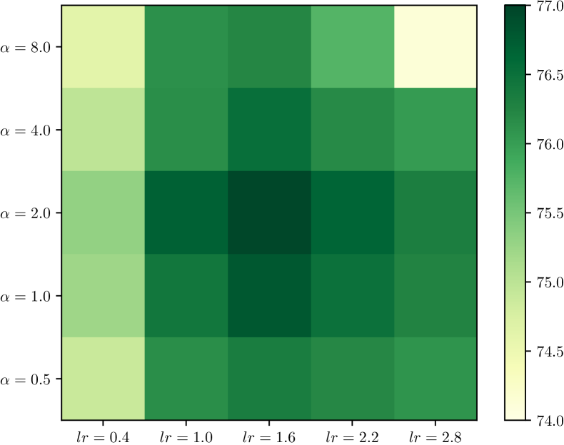
Section 2.2 and 2.3 investigate the two main mechanisms of weight decay: (1) for layers followed by normalizations(mainly convolution layers), affecting ELR (2) for final fully-connected layers, affecting cross-boundary risk. Algo 1@FixNorm-FC (refered to FixNorm for simplicity) unifies these two mechanisms and directly controls their effects through hyper-parameters $lr$ and $\alpha$. While these two mechanisms both affect generalization performance, it is important to know how they are correlated, which will determine how to tune two hyper-parameters. To verify this, we grid search $lr$ and $\alpha$ and show the corresponding top-1 accuracy in Fig 4. It clearly shows that the best $lr$ does not depends on the value of $\alpha$ and vice versa. This suggests that we can tune $lr$ and $\alpha$ independently, which will greatly reduce the cost.

Instead of using existing hyper-parameter optimization(HPO) methods, we propose a simple yet effective approach to tune $lr$ and $\alpha$. We introduce two priors to efficiently tune $lr$.

• Top-1 accuracy is approximately a convex function for $lr$

• The best $lr$ for shorter training is usually larger than that for longer training

The first prior is mainly an empirical finding, while the second one may be partially explained by the correlation between generalization performance and weight distance from their initialization(Hoffer et al., 2017): shorter training may require larger $lr$ to travel far enough from the initialization in weight space to generalize well. These two priors motivate us to use best lr under shorter training as an upper bound for that under longer training. This strategy can adaptively shrink the search range and let us locate the best $lr$ in a wide range with relatively low cost. After the best $lr$ is found, we simply fix it and grid search for the best $\alpha$. The overall method can be summarized in Algo 4(tuned FixNorm).

Algorithm 4 Tuning $lr$ and $\alpha$ for FixNorm training

Input: number of $lr$ tuning rounds $N$, learning rate range $[lr_{min},lr_{max}]$, learning rate split number $K$, training steps of each $lr$ tuning round $\bm{T}=[T_{0},T_{1},...,T_{N-1}]$ where $T_{i}\leq T_{i+1}$, alpha candidates $[\alpha_{0},\alpha_{1},...,\alpha_{m-1}]$
Output: $\alpha_{best}$, $lr_{best}$, $acc_{best}$
Initialization: $\alpha_{best}=\alpha_{0}$, $lr_{best}=\text{NULL}$, $acc_{best}=0$

1: 

2:Phase 1 - Find $lr_{best}$

3: 

4:for $r$ in 0, …, $N-1$ do

5:     $\bm{LR}\leftarrow\text{UniformSplit}(lr_{min},lr_{max},K)$

6:     $\bm{Acc}\leftarrow\left\{\text{FixNormTrain}(LR_{k},\alpha_{best},T_{r})|\ k\in\left\{0,...,K-1\right\}\right\}$

7:     $idx\leftarrow\arg\max\bm{Acc}$

8:     $lr_{max}\leftarrow\bm{LR}_{idx}$

9:     if $\bm{Acc}_{idx}>acc_{best}$ then

10:         $acc_{best}\leftarrow\bm{Acc}_{idx}$

11:         $lr_{best}\leftarrow\bm{LR}_{idx}$

12:     end if

13:end for

14: 

15:Phase 2 - Find $\alpha_{best}$

16: 

17:$\bm{Acc}\leftarrow\left\{\text{FixNormTrain}(lr_{best},\alpha_{i},T_{N-1})|\ i\in\left\{1,...,m-1\right\}\right\}$

18:$idx\leftarrow\arg\max\bm{Acc}$

19:if $\bm{Acc}_{idx}>acc_{best}$ then

20:     $acc_{best}\leftarrow\bm{Acc}_{idx}$

21:     $\alpha_{best}\leftarrow\alpha_{idx}$

22:end if

3 Experiments

General setups

We perform experiments on ImageNet classification task (Deng et al., 2009) which contains 1.28 million training images and 50000 validation images. Our general training settings are mainly adapted from He et al. (2019), which include Nesterov Accelerated Gradient (NAG) descent(Nesterov, 1983), one-cycle cosine learning rate decay(Loshchilov & Hutter, 2016) with linear warmup at first 4 epochs(Goyal et al., 2017) and label smoothing with $\epsilon=0.1$(Szegedy et al., 2016). We do not use mixup augmentation(Zhang et al., 2017). All the models are trained on 16 Nvidia V100 GPUs with a total batch size of 1024. Other settings follow reference implementations of each model. We leave experiments on MS COCO and Cityscapes in supplementary materials.

FixNorm tuning setups

For Algo 4, we set $N=2$, learning rate range $[0.2,3.2]$, $K=5$, $\bm{T}=[0.2T_{max},T_{max}]$ where $T_{max}$ is the max training steps, $\alpha$ candidates [0.5, 1.0, 2.0, 4.0, 8.0, 16.0]. The search contains two $lr$ tuning rounds and one $\alpha$ tuning round. The total computational resources consumed are $K\times 0.2T_{max}+K\times T_{max}+(6-1)\times T_{max}=11T_{max}$, which is 11 times of a single training process.

3.1 Tuned FixNorm on ResNet50-D and MobileNetV2

To demonstrate the effectiveness of our method, we first apply Algo 4 on two well-studied architectures: ResNet50-D(He et al., 2019) and MobileNetV2(Sandler et al., 2018). We follow He et al. (2019) and train 120 epochs for ResNet50-D and 150 epochs for MobileNetV2. Their reference top-1 accuracies reported are 78.37% and 72.04%. We also adopt Bayesian Optimization(BO)(Snoek et al., 2012) to search learning rate and weight decay under normal weight decay training (BO+WD) for these models. We use the same learning rate range $[0.2,3.2]$ for BO, and the weight decay range is set to $[0.00001,0.0005]$. Results are shown in Table 1.

Table 1: Results for tuned FixNorm and BO+WD training

	Tuned FixNorm			BO + WD			Reference
	$lr$	$\alpha$	top-1(%)	$lr$	$\lambda$	top-1(%)	$lr$	$\lambda$	top-1(%)
ResNet50-D	1.4	0.5	78.62	0.53	8.6e-5	78.53	0.4	1e-4	78.37
MobileNetV2	0.5	16.0	73.20	0.64	2.2e-5	72.84	0.2	4e-5	72.04

As in Table 1, both tuned FixNorm and BO+WD outperform reference settings by a clear margin. Although the reference settings have already been heavily refined in He et al. (2019), our method still brings substantial improvements. We further compare tuned FixNorm and BO+WD in Fig 5 left. Our method shows two advantages compared to BO+WD. First, our method finds better solutions at lower cost. The cost of our method is 11 times of normal training while BO+WD requires 25 and 35, while our final results are even better than that found by BO+WD. Second, our method is more stable and barely needs meta-tuning. BO itself has lots of tunable meta hyper-parameters (Lindauer et al., 2019) and it requires expert knowledge to tune them. While we use exactly the same FixNorm tuning setups for all the experiments, including in Table 2. These setups are intuitive and the method performs consistently well across all the settings.

Figure 5: Left: search progress for FixNorm and BO+WD Middle: FixNorm search details for ResNet50-D Right: FixNorm search details for MobileNetV2

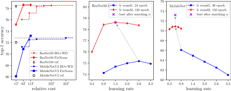
To better understand our method, we show more details about tuned FixNorm in Fig 5 middle and right, for ResNet50-D and MobileNetV2 respectively. There are two $lr$ searching rounds and one $\alpha$ searching round under our setups. In the first $lr$ round, both experiments starts with $lr$ values in [0.8, 1.4, 2.0, 2.6, 3.2] (which are the uniform split points of initial range [0.2, 3.2]) and train for $1/5$ total epochs(24 epochs and 30 epochs respectively). Best $lr$ values are very different in this round: $lr_{1}=2.6$ for ResNet50-D and $lr_{1}=0.8$ for MobileNetV2. Taking these values as new upper bound, [0.2, $lr_{1}$] are further split and corresponding $lr$ values are evaluated in the second round, for full total epochs. The best $lr$ values are 1.4 and 0.5 in this round. These values are fixed and then $\alpha$ is searched. For ResNet50-D, the initial $\alpha=0.5$ is already the best, while for MobileNetV2 a better $\alpha=16.0$ is founded. From Fig 5 one can find the patterns match two priors introduced in section 2.4.

3.2 New state-of-the-arts with tuned FixNorm

Many powerful networks have been proposed recently. These networks usually adopt many tricks and therefore hard to tune. To fully exploit the capabilities of these networks, we apply tuned FixNorm to further optimize them. We also apply advanced tricks to basic models like MobileNetV2 and ResNet50-D. These tricks are used by EfficientNet(Tan & Le, 2019), including SE-layer(Hu et al., 2018), swish activation(Ramachandran et al., 2017), stochastic depth training(Huang et al., 2016) and AutoAugment preprocessing(Cubuk et al., 2019). From Table 2, we can find that:

• Our method consistently outperforms reference settings. Strong baselines like EfficientNet can be further improved by our method, specifically +0.4% and +0.3% for B0 and B1.

• Tunning matters. When simply apply tricks to MobileNetV2 and scale to the same FLOPS with B0 and B1, tuned FixNorm achieves 77.4% and 79.18% top-1 accuracy, while default training settings only get 76.72 and 78.75. This difference can lead to unreliable conclusions when compared to EfficientNet.

• Best $lr$ and $\alpha$ are different among models, even for the same model with different settings. This may suggest that we should tune for each setting to fully exploit their performance.

Table 2: Results with tuned FixNorm models with * are applied with tricks, †means the result is obtained using $lr$ and $\lambda$ from basic settings(MobileNetV2 150 and ResNet50-D 120)

Model	#Epochs	Top-1	Top-1 (ref.)	#Params	#FLOPS	$lr$	$\alpha$
MobileNetV2	150	73.20	72.04	3.5M	300M	0.5	16.0
MobileNetV2	350	73.97	73.38†	3.5M	300M	0.35	8.0
EfficientNet-B0	350	77.72	77.30	5.3M	384M	0.5	4.0
EfficientNet-B1	350	79.52	79.20	7.8M	685M	0.8	8.0
MobileNetV2$\times$1.12*	350	77.40	76.72†	4.7M	386M	0.5	8.0
MobileNetV2$\times$1.54*	350	79.18	78.75†	8.0M	682M	0.65	4.0
ResNet50-D	120	78.62	78.37	25.6M	4.3G	1.4	0.5
ResNet50-D	350	79.29	79.04†	25.6M	4.3G	1.1	0.5
ResNet50-D*	350	81.27	80.80†	28.1M	4.3G	1.1	1.0

4 Related works

Due to the page limit, we only highlight the most related works in this section and leave other works in supplementary materials.

Understanding weight decay

Recently, a series of works (Van Laarhoven, 2017; Zhang et al., 2018; Hoffer et al., 2018) propose that when combined with normalizations, the main effect of weight decay is increasing ELR, which is contrary to the previous understanding and motivates new perspectives. Van Laarhoven (2017) first introduces the ELR hypothesis and provides derivations for different optimizers, while both Hoffer et al. (2018); Zhang et al. (2018) give additional evidence supporting the hypothesis. Hoffer et al. (2018) also proposes norm-bounded Weight Normalization, which fixes the norm of each convolution layer separately. By doing this, their method fixes the ELR of each layer, which highly depends on the initialization of each layer. Differently, we fix the norm of all convolution layers as a whole and maintains the global ELR, which is more robust and demonstrates SOTA performance on large scale experiments. Layer-wise ELR controlling is an interesting problem and may lead to new perspectives for weight initialization techniques. Similar to Hoffer et al. (2018), Xiang et al. (2019) also proposes modifications to Weight Normalization based on ELR hypothesis. They identify the problems when using weight decay with Weight Normalization, and propose $\epsilon-$shifted $L_{2}$ regularizer to constrain weight norm to $\epsilon$ with coefficient $\lambda$. Beyond ELR hypothesis, Li & Arora (2019) derives a closed-form between learning rate, weight decay and momentum, and proposes an exponentially increasing learning rate schedule. Their work mainly discusses the linkage of three hyper-parameters, while our work focuses on the underlying mechanisms of weight decay. Except for the ELR hypothesis, Loshchilov & Hutter (2017) identifies problems when applying weight decay to Adam optimizer, which improves generalization performance and decouples it from learning rate. All these works bring interesting perspectives for understanding weight decay, yet our work has distinct differences and contributions. First, our work investigates the effect on final FC layers and find a new mechanism that complements the understanding of weight decay on generalization performance, which is mostly ignored by previous works. Second, our method including FixNorm and the tuning method are both concise and effective, and demonstrate SOTA performance on large scale datasets.

5 Conclusion

In this paper, we find a new mechanism of weight decay on final FC layers, which affects generalization performance by controlling cross-boundary risk. This new mechanism complements the ELR hypothesis and gives a better understanding of weight decay. We propose a new training method called FixNorm, which discards weight decay and directly controls the two mechanisms. We also propose an effective, efficient and robust method to tune hyperparameters of FixNorm, which can consistently find near-optimal solutions in a few trials. Experiments on large scale datasets demonstrate our methods, and a series of SOTA baselines are established for fair comparisons. We believe this work brings new perspectives and may motivate interesting ideas like controlling layer-wise ELR and automatically adjusting cross-boundary risk.

Appendix A Appendix

A.1 Algorithms

In section 2.3, we apply three modifications to Algo 1: (1) replace original FC layer with WN-FC layer; (2) replace $\bm{W}^{\text{Conv}}$ in line 7 of Algo 6 with $\bm{W}^{\text{Conv+FC}}$; (3) set $\lambda^{\text{FC}}=0$. This modified algorithm is denoted as Algo 1@WN-FC. Here we show the full Algo 1@WN-FC as follows:

Algorithm 5 @WN-FC

Input: initial learning rate $lr$, total steps $T$, momentum $\mu$, training samples $\bm{x}$, corresponding labels $\bm{y}$
Replace: replace original FC layer with WN-FC layer
Initialization: velocity $\bm{V}_{0}\leftarrow\bm{0}$, random initialize weight vector $\bm{W_{0}}$

1:for $t$ in 0, …, $T-1$ do

2:     $\bm{x},\bm{y}$ $\leftarrow$ BatchSampler($t$)

3:     $\widehat{\mathcal{L}}_{t}(\bm{W}_{t})\leftarrow\sum\mathcal{L}(f(x;\bm{W}_{t}),y)$

4:     $\bm{V}_{t+1}\leftarrow\mu\bm{V}_{t}+\nabla\widehat{\mathcal{L}}_{t}(\bm{W}_{t})$

5:     $\eta_{t}\leftarrow$ GetLRScheduleMultiplier$(t)$

6:     $\bm{W}_{t+1}\leftarrow\bm{W}_{t}-lr\times\eta_{t}\times\bm{V}_{t+1}$

7:     $\bm{W}^{\text{Conv+FC}}_{t+1}\leftarrow\frac{\bm{W}^{\text{Conv+FC}}_{t+1}}{\|\bm{W}^{\text{Conv+FC}}_{t+1}\|_{2}}\|\bm{W}^{\text{Conv+FC}}_{0}\|_{2}$

8:end for

The Algo 1@FixNorm-FC is similar to Algo 1@WN-FC, the only different is that we use FixNorm-FC layer instead of WN-FC layer. The full algorithm is shown as follows:

Algorithm 6 @FixNorm-FC

Input: initial learning rate $lr$, total steps $T$, momentum $\mu$, training samples $\bm{x}$, corresponding labels $\bm{y}$
Replace: replace original FC layer with FixNorm-FC layer
Initialization: velocity $\bm{V}_{0}\leftarrow\bm{0}$, random initialize weight vector $\bm{W_{0}}$

1:for $t$ in 0, …, $T-1$ do

2:     $\bm{x},\bm{y}$ $\leftarrow$ BatchSampler($t$)

3:     $\widehat{\mathcal{L}}_{t}(\bm{W}_{t})\leftarrow\sum\mathcal{L}(f(x;\bm{W}_{t}),y)$

4:     $\bm{V}_{t+1}\leftarrow\mu\bm{V}_{t}+\nabla\widehat{\mathcal{L}}_{t}(\bm{W}_{t})$

5:     $\eta_{t}\leftarrow$ GetLRScheduleMultiplier$(t)$

6:     $\bm{W}_{t+1}\leftarrow\bm{W}_{t}-lr\times\eta_{t}\times\bm{V}_{t+1}$

7:     $\bm{W}^{\text{Conv+FC}}_{t+1}\leftarrow\frac{\bm{W}^{\text{Conv+FC}}_{t+1}}{\|\bm{W}^{\text{Conv+FC}}_{t+1}\|_{2}}\|\bm{W}^{\text{Conv+FC}}_{0}\|_{2}$

8:end for

A.2 Derivations

The complete derivations of equation 8 are as follows. $\mathcal{L}$ denotes the softmax cross-entropy loss, $s_{i}=\frac{x^{\mathsf{T}}\bm{W}_{i}}{\|\bm{W}\|_{2}}g$ denotes the logits value of class $i$, $p_{i}$ denotes the probability of class $i$, $k$ for the label class and $j$ for other classes. We have,

$$\mathcal{L}(x,k) =-\log p_{k}=-\log\frac{e^{s_{k}}}{\sum e^{s_{i}}}$$ (11)

We first derive $\frac{\partial p_{k}}{\partial s_{k}}$:

$$\frac{\partial p_{k}}{\partial s_{k}} =\frac{e^{s_{k}}\sum e^{s_{j}}-e^{s_{k}}e^{s_{k}}}{\left(\sum e^{s_{j}}\right)^{2}}$$ (13)

$$=\frac{e^{s_{k}}}{\sum e^{s_{j}}}-\left(\frac{e^{s_{k}}}{\sum e^{s_{j}}}\right)^{2}$$ (14)

$$=p_{k}-{p_{k}}^{2}$$ (15)

$$=p_{k}(1-p_{k})$$ (16)

also for $j\neq k$, we have,

$$\frac{\partial p_{k}}{\partial s_{j}} =\frac{-e^{s_{k}}e^{s_{j}}}{\left(\sum e^{s_{i}}\right)^{2}}$$ (17)

$$=-p_{k}p_{j}$$ (18)

combine them with $\frac{\partial s_{i}}{\partial x}=\frac{\bm{W}_{i}}{\|\bm{W}\|_{2}}g$, we have,

$$\frac{\partial p_{k}}{\partial x} =\frac{\partial p_{k}}{\partial s_{k}}\frac{\partial s_{k}}{\partial x}+\sum_{j\neq k}\frac{\partial p_{k}}{\partial s_{j}}\frac{\partial s_{j}}{\partial x}$$ (19)

$$=p_{k}(1-p_{k})\frac{\bm{W}_{k}}{\|\bm{W}\|_{2}}g+\sum_{j\neq k}-p_{k}p_{j}\frac{\bm{W}_{j}}{\|\bm{W}\|_{2}}g$$ (20)

$$=\frac{p_{k}g}{\|\bm{W}\|_{2}}\left((1-p_{k})\bm{W}_{k}+\sum_{j\neq k}-p_{j}\bm{W}_{j}\right)$$ (21)

$$=\frac{p_{k}g}{\|\bm{W}\|_{2}}\left(\bm{W}_{k}+\sum-p_{i}\bm{W}_{i}\right)$$ (22)

$$=\frac{p_{k}g}{\|\bm{W}\|_{2}}\left(\sum p_{i}(\bm{W}_{k}-\bm{W}_{i})\right)$$ (23)

$$=\frac{p_{k}g}{\|\bm{W}\|_{2}}\left(\sum_{j\neq k}p_{j}(\bm{W}_{k}-\bm{W}_{j})\right)$$ (24)

and finally,

$$-\frac{\partial\mathcal{L}(x,k)}{\partial x} =-\frac{\partial\mathcal{L}(x,k)}{\partial p_{k}}\frac{\partial p_{k}}{\partial x}$$ (26)

$$=\frac{1}{p_{k}}\frac{p_{k}g}{\|\bm{W}\|_{2}}\sum_{j\neq k}p_{j}(\bm{W}_{k}-\bm{W}_{j})$$ (27)

$$=\frac{g}{\|\bm{W}\|_{2}}\sum_{j\neq k}p_{j}(\bm{W}_{k}-\bm{W}_{j})$$ (28)

A.3 More Details

Parameters other than convolution and FC weights

For modern CNNs like ResNet or MobileNet, the majority of parameters come from weights of convolution and FC layers. Other parameters are mainly biases and $\gamma$ and $\beta$ of BN layers. As in He et al. (2019), the no-bias-decay strategy is applied to avoid overfitting, which does not use weight decay on these parameters. We empirically find that this strategy does not harm performance, so we adopt this strategy in our FixNorm method, which means we do not fix the norm of biases and $\gamma$ and $\beta$ parameters. Experiments in Table 2 also include architectures with SE-blocks, which have FC layers that are not followed by normalizations. Since these layers are not directly followed by softmax cross-entropy loss, we find that they do not suffer from the problem identified in section 2.3. So we simply replace these layers with WN-FC layers and add the weights into the norm-fixing process. In summary, our FixNorm method considers weights of convolution layers, final FC-layers, and FC layers of SE-blocks. Other parameters like biases and $\gamma$ and $\beta$ of BN layers are excluded from the norm fixing process.

A.4 More results on segmentation and object detection

A.4.1 Extending FixNorm-FC for pixel-wise classification

The FixNorm-FC is proposed to replace the original final FC layer in classification tasks. There are other forms of classification tasks that do not use FC layers, such as segmentation and object detection. For segmentation, the models are usually fully convolutional and the last convolution layer is used for pixel-wise classification. This also applies to Region Proposal NetworksRen et al. (2015) used in object detection or methods that produce dense detections like RetinaNetLin et al. (2017). These tasks still share the nature of the classification task, therefore the cross-boundary risk still needs to be controlled. Our FixNorm-FC layer can be easily extended to these tasks because the final convolution layer can be viewed as a normal FC layer that shares weight across spatial positions. Denote the weight of the final convolution layer as $\bm{W}^{\text{Conv}}$ with shape $[c_{out},c_{in},k_{h},k_{w}]$, we define,

$$\text{FixNorm-Conv}(x;\bm{W}^{\text{Conv}},g,\alpha)=\frac{\text{Conv}(x,\bm{W}^{\text{Conv}})}{\|\bm{W}^{\text{Conv}}\|_{2}}\times\min(g,\alpha*\sqrt{c_{out}})$$ (29)

This layer is a straight forward extension of FixNorm-FC layer, which will be used in experiments on segmentation and detection later.

A.4.2 Experiments on Cityscapes

Setups

The Cityscapes datasetCordts et al. (2016) is a task for urban scene understanding. We follow the basic training settings in Yuan & Wang (2018). We use 2975 images for training and 500 images for validation. The initial learning rate is set as 0.01 and weight decay as 0.0005. The original image size is 1024$\times$2048 and we use crop size of 769$\times$769. All the models are trained on 4 Nvidia V100 GPUs for 40000 iterations with a total batch size of 8. The poly learning rate policy is used. We use the ResNet-101 + Base-OCYuan & Wang (2018) as the baseline model.

Modifications

We replace the last convolution layer with FixNorm-Conv when trained with our FixNorm method.

FixNorm tuning setups

The main settings are the same with that on ImageNet, such as $N=2$, $K=5$, $T=[0.2T_{max},T_{max}]$, $\alpha$ candidates as [0.5, 1.0, 2.0, 4.0, 8.0, 16.0]. The only difference is that we adapt the learning rate range to [0.005, 0.1]. The reason is that the models are finetuned on a pre-trained model from ImageNet, therefore the default learning rate is smaller.

The results are shown in table 3. Tuned FixNorm clearly outperforms the baseline and the improvements are larger when the cosine learning rate is applied.

Table 3: Results with tuned FixNorm on Cityscapes

Model	#Iters	Val. mIoU(%)	hyperparameters
baseline	40000	78.7	lr=0.01, wd=0.0005
baseline w/ cosine lr	40000	78.3	lr=0.01, wd=0.0005
tuned FixNorm	40000	79.4	lr=0.0335, $\alpha=1.0$
tuned FixNorm w/ cosine lr	40000	79.7	lr=0.043, $\alpha=1.0$

A.4.3 Experiments on MS COCO

Setups

To verify our tuned FixNorm method on object detection task, we train RetinaNetLin et al. (2017) on MS COCOLin et al. (2014). We following common practice and use the COCO trainval35k split, and report results on the minival split. We use the ResNet50-FPN backbone, while the base ResNet50 model is pre-trained on ImageNet. The RetinaNet is trained with stochastic gradient descent(SGD) on 8 Nvidia V100 GPUs with a total batch size of 16. The models are trained for 90k iterations with default learning rate 0.01, which is then divided by 10 at 60k and 80k iterations. The default weight decay is 0.0001. The $\alpha_{focal}$ is set to 0.25 and the $\gamma_{focal}$ is set to 2.0. The standard smooth $L_{1}$ loss is used for box regression. We use horizontal image flipping as the only data augmentation, and the image scale is set to 800 pixels.

Modifications

To make the RetinaNet compatible with our method, we add Weight Normalization layers to all the convolution layers that are not followed by normalizations (include layers in FPN and classification subnet and bounding-box prediction subnet), for all the models. We also replace the last convolution layer of the classification subnet with FixNorm-Conv when trained with our FixNorm method. The last convolution layer of the bounding-box prediction subnet is used for regression task, which does not suffer from the problem identified in section 2.3, so we do not replace it with FixNorm-Conv.

FixNorm tuning setups

The main settings are the same with that on ImageNet, such as $N=2$, $K=5$, $T=[0.2T_{max},T_{max}]$, $\alpha$ candidates as [0.5, 1.0, 2.0, 4.0, 8.0, 16.0]. As the models are finetuned on a pre-trained model, we use the same learning rate range of [0.005, 0.1] as in segmentation experiments.

The results are shown in table 4. Tuned FixNorm clearly outperforms the baseline and the improvements are larger when the cosine learning rate is applied.

Table 4: Results with tuned FixNorm on MS COCO

Model	#Iters	Val. AP(%)	hyperparameters
baseline	90000	36.5	lr=0.01, wd=0.0001
baseline w/ cosine lr	90000	36.2	lr=0.01, wd=0.0001
tuned FixNorm	90000	36.9	lr=0.0145, $\alpha=0.5$
tuned FixNorm w/ cosine lr	90000	37.1	lr=0.0145, $\alpha=0.5$

A.5 Additional related works

Hyperparameter Optimization (HPO). Hyperparameter Optimization is an important topic for effectively training DNNs. One straight forward method is grid search, which is only affordable for a very limited number of hyperparameters since the combinations grow exponentially. Random search(Bull, 2011) is a popular alternative that select hyperparameter combinations randomly, which can be more efficient when the resource is constrained. Bayesian Optimization(BO) (Brochu et al., 2010) further improves efficiency by using a model that is built on historical information to guide the selection. Hyperband(Li et al., 2017) allocates different budgets to random configurations and rejects bad ones according to the performance obtained under low budgets. BOHB (Falkner et al., 2018) combines BO with Hyperband to select more promising configurations. Both Hyperband and BOHB highly relies on the assumption that performance under different budgets is consistent. However, this assumption is not always true and these methods may suffer from the low rank-correlation of performance under different budgets(Ying et al., 2019). While these methods are universal black-box optimization methods, our tuning method leverages more priors of hyperparameters. Our method suggests that with a better understanding of the underlying mechanisms, we can develop a method that is both effective and efficient.

References

- Bös (1996) Siegfried Bös. Optimal weight decay in a perceptron. In International Conference on Artificial Neural Networks, pp. 551–556. Springer, 1996.
- Bos & Chug (1996) Siegfried Bos and E Chug. Using weight decay to optimize the generalization ability of a perceptron. In Proceedings of International Conference on Neural Networks (ICNN’96), volume 1, pp. 241–246. IEEE, 1996.
- Brochu et al. (2010) Eric Brochu, Vlad M Cora, and Nando De Freitas. A tutorial on bayesian optimization of expensive cost functions, with application to active user modeling and hierarchical reinforcement learning. arXiv preprint arXiv:1012.2599, 2010.
- Bull (2011) Adam D Bull. Convergence rates of efficient global optimization algorithms. Journal of Machine Learning Research, 12(Oct):2879–2904, 2011.
- Cordts et al. (2016) Marius Cordts, Mohamed Omran, Sebastian Ramos, Timo Rehfeld, Markus Enzweiler, Rodrigo Benenson, Uwe Franke, Stefan Roth, and Bernt Schiele. The cityscapes dataset for semantic urban scene understanding. In Proc. of the IEEE Conference on Computer Vision and Pattern Recognition (CVPR), 2016.
- Cubuk et al. (2019) Ekin D Cubuk, Barret Zoph, Dandelion Mane, Vijay Vasudevan, and Quoc V Le. Autoaugment: Learning augmentation strategies from data. In Proceedings of the IEEE conference on computer vision and pattern recognition, pp. 113–123, 2019.
- Deng et al. (2009) Jia Deng, Wei Dong, Richard Socher, Li-Jia Li, Kai Li, and Li Fei-Fei. Imagenet: A large-scale hierarchical image database. In 2009 IEEE conference on computer vision and pattern recognition, pp. 248–255. Ieee, 2009.
- Falkner et al. (2018) Stefan Falkner, Aaron Klein, and Frank Hutter. Bohb: Robust and efficient hyperparameter optimization at scale. arXiv preprint arXiv:1807.01774, 2018.
- Goyal et al. (2017) Priya Goyal, Piotr Dollár, Ross Girshick, Pieter Noordhuis, Lukasz Wesolowski, Aapo Kyrola, Andrew Tulloch, Yangqing Jia, and Kaiming He. Accurate, large minibatch sgd: Training imagenet in 1 hour. arXiv preprint arXiv:1706.02677, 2017.
- He et al. (2016) Kaiming He, Xiangyu Zhang, Shaoqing Ren, and Jian Sun. Deep residual learning for image recognition. In Proceedings of the IEEE conference on computer vision and pattern recognition, pp. 770–778, 2016.
- He et al. (2019) Tong He, Zhi Zhang, Hang Zhang, Zhongyue Zhang, Junyuan Xie, and Mu Li. Bag of tricks for image classification with convolutional neural networks. In The IEEE Conference on Computer Vision and Pattern Recognition (CVPR), June 2019.
- Hoffer et al. (2017) Elad Hoffer, Itay Hubara, and Daniel Soudry. Train longer, generalize better: closing the generalization gap in large batch training of neural networks. In I. Guyon, U. V. Luxburg, S. Bengio, H. Wallach, R. Fergus, S. Vishwanathan, and R. Garnett (eds.), Advances in Neural Information Processing Systems 30, pp. 1731–1741. Curran Associates, Inc., 2017. URL http://papers.nips.cc/paper/6770-train-longer-generalize-better-closing-the-generalization-gap-in-large-batch-training-of-neural-networks.pdf.
- Hoffer et al. (2018) Elad Hoffer, Ron Banner, Itay Golan, and Daniel Soudry. Norm matters: efficient and accurate normalization schemes in deep networks. In Advances in Neural Information Processing Systems, pp. 2160–2170, 2018.
- Hu et al. (2018) Jie Hu, Li Shen, and Gang Sun. Squeeze-and-excitation networks. In Proceedings of the IEEE conference on computer vision and pattern recognition, pp. 7132–7141, 2018.
- Huang et al. (2016) Gao Huang, Yu Sun, Zhuang Liu, Daniel Sedra, and Kilian Q Weinberger. Deep networks with stochastic depth. In European conference on computer vision, pp. 646–661. Springer, 2016.
- Ioffe & Szegedy (2015) Sergey Ioffe and Christian Szegedy. Batch normalization: Accelerating deep network training by reducing internal covariate shift. arXiv preprint arXiv:1502.03167, 2015.
- Krizhevsky et al. (2012) Alex Krizhevsky, Ilya Sutskever, and Geoffrey E Hinton. Imagenet classification with deep convolutional neural networks. In Advances in neural information processing systems, pp. 1097–1105, 2012.
- Krogh & Hertz (1992) Anders Krogh and John A Hertz. A simple weight decay can improve generalization. In Advances in neural information processing systems, pp. 950–957, 1992.
- Li et al. (2017) Lisha Li, Kevin Jamieson, Giulia DeSalvo, Afshin Rostamizadeh, and Ameet Talwalkar. Hyperband: A novel bandit-based approach to hyperparameter optimization. The Journal of Machine Learning Research, 18(1):6765–6816, 2017.
- Li & Arora (2019) Zhiyuan Li and Sanjeev Arora. An exponential learning rate schedule for deep learning. arXiv preprint arXiv:1910.07454, 2019.
- Lin et al. (2014) Tsung-Yi Lin, Michael Maire, Serge Belongie, James Hays, Pietro Perona, Deva Ramanan, Piotr Dollár, and C Lawrence Zitnick. Microsoft coco: Common objects in context. In European conference on computer vision, pp. 740–755. Springer, 2014.
- Lin et al. (2017) Tsung-Yi Lin, Priya Goyal, Ross Girshick, Kaiming He, and Piotr Dollár. Focal loss for dense object detection. In Proceedings of the IEEE international conference on computer vision, pp. 2980–2988, 2017.
- Lindauer et al. (2019) Marius Lindauer, Matthias Feurer, Katharina Eggensperger, André Biedenkapp, and Frank Hutter. Towards assessing the impact of bayesian optimization’s own hyperparameters. arXiv preprint arXiv:1908.06674, 2019.
- Loshchilov & Hutter (2016) Ilya Loshchilov and Frank Hutter. Sgdr: Stochastic gradient descent with warm restarts. arXiv preprint arXiv:1608.03983, 2016.
- Loshchilov & Hutter (2017) Ilya Loshchilov and Frank Hutter. Decoupled weight decay regularization. arXiv preprint arXiv:1711.05101, 2017.
- Nesterov (1983) Yurii E Nesterov. A method for solving the convex programming problem with convergence rate o (1/k^ 2). In Dokl. akad. nauk Sssr, volume 269, pp. 543–547, 1983.
- Ramachandran et al. (2017) Prajit Ramachandran, Barret Zoph, and Quoc V Le. Searching for activation functions. arXiv preprint arXiv:1710.05941, 2017.
- Ren et al. (2015) Shaoqing Ren, Kaiming He, Ross Girshick, and Jian Sun. Faster r-cnn: Towards real-time object detection with region proposal networks. In Advances in neural information processing systems, pp. 91–99, 2015.
- Salimans & Kingma (2016) Tim Salimans and Durk P Kingma. Weight normalization: A simple reparameterization to accelerate training of deep neural networks. In Advances in neural information processing systems, pp. 901–909, 2016.
- Sandler et al. (2018) Mark Sandler, Andrew Howard, Menglong Zhu, Andrey Zhmoginov, and Liang-Chieh Chen. Mobilenetv2: Inverted residuals and linear bottlenecks. In Proceedings of the IEEE conference on computer vision and pattern recognition, pp. 4510–4520, 2018.
- Snoek et al. (2012) Jasper Snoek, Hugo Larochelle, and Ryan P Adams. Practical bayesian optimization of machine learning algorithms. In F. Pereira, C. J. C. Burges, L. Bottou, and K. Q. Weinberger (eds.), Advances in Neural Information Processing Systems 25, pp. 2951–2959. Curran Associates, Inc., 2012. URL http://papers.nips.cc/paper/4522-practical-bayesian-optimization-of-machine-learning-algorithms.pdf.
- Szegedy et al. (2016) Christian Szegedy, Vincent Vanhoucke, Sergey Ioffe, Jon Shlens, and Zbigniew Wojna. Rethinking the inception architecture for computer vision. In Proceedings of the IEEE conference on computer vision and pattern recognition, pp. 2818–2826, 2016.
- Tan & Le (2019) Mingxing Tan and Quoc V Le. Efficientnet: Rethinking model scaling for convolutional neural networks. arXiv preprint arXiv:1905.11946, 2019.
- Van Laarhoven (2017) Twan Van Laarhoven. L2 regularization versus batch and weight normalization. arXiv preprint arXiv:1706.05350, 2017.
- Xiang et al. (2019) Li Xiang, Chen Shuo, Xia Yan, and Yang Jian. Understanding the disharmony between weight normalization family and weight decay: shifted regularizer. arXiv preprint arXiv:1911.05920, 2019.
- Ying et al. (2019) Chris Ying, Aaron Klein, Esteban Real, Eric Christiansen, Kevin Murphy, and Frank Hutter. Nas-bench-101: Towards reproducible neural architecture search. arXiv preprint arXiv:1902.09635, 2019.
- Yuan & Wang (2018) Yuhui Yuan and Jingdong Wang. Ocnet: Object context network for scene parsing. arXiv preprint arXiv:1809.00916, 2018.
- Zhang et al. (2018) Guodong Zhang, Chaoqi Wang, Bowen Xu, and Roger Grosse. Three mechanisms of weight decay regularization. arXiv preprint arXiv:1810.12281, 2018.
- Zhang et al. (2017) Hongyi Zhang, Moustapha Cisse, Yann N Dauphin, and David Lopez-Paz. mixup: Beyond empirical risk minimization. arXiv preprint arXiv:1710.09412, 2017.