Variational Rejection Particle Filtering

Abstract

We present a variational inference (VI) framework that unifies and leverages sequential Monte-Carlo (particle filtering) with approximate rejection sampling to construct a flexible family of variational distributions. Furthermore, we augment this approach with a resampling step via Bernoulli race, a generalization of a Bernoulli factory, to obtain a low-variance estimator of the marginal likelihood. Our framework, Variational Rejection Particle Filtering (VRPF), leads to novel variational bounds on the marginal likelihood, which can be optimized efficiently with respect to the variational parameters and generalizes several existing approaches in the VI literature. We also present theoretical properties of the variational bound and demonstrate experiments on various models of sequential data, such as the Gaussian state-space model and variational recurrent neural net (VRNN), on which VRPF outperforms various existing state-of-the-art VI methods.

1 Introduction

Exact inference in latent variable models (LVM) is usually intractable. Recently VI (Blei et al., 2017) methods have received considerable interest for LVMs due to their excellent scalability on large-scale datasets. This is made possible thanks to scalable amortized VI methods (Kingma & Welling, 2013; Ranganath et al., 2014) and stochastic VI (Hoffman et al., 2013). In particular, VI maximizes a lower bound on the log marginal likelihood to obtain an approximate posterior. Constructing a low variance estimator of the marginal likelihood is desirable due to a tighter VI bound and yields a better approximation to the target posterior (Domke & Sheldon, 2019). The two basic schemes for constructing a low variance estimator of the marginal likelihood are based on sampling methods (MCMC, rejection sampling) (Salimans et al., 2015; Ruiz & Titsias, 2019; Hoffman, 2017; Grover et al., 2018) or particle-based approximation (e.g., sequential Monte-Carlo (SMC) and importance sampling (IS)) (Burda et al., 2015; Maddison et al., 2017).

In this paper, we develop a novel VI bound, VRPF (Variational Rejection Particle Filtering), which is based on unifying a particle approximation with a sampling-based approach. In particular, the proposed bound formulates an efficient variational proposal via particle approximation followed by further refinement through a sampling-based technique. To accomplish this, we leverage the idea of partial rejection control (PRC) (Peters et al., 2012; Liu et al., 1998), an approximate rejection sampling step, within the framework of SMC, which is a particle approximation, and exploit their synergy to develop a flexible family of approximate posteriors. Note that VRPF does not employ sampling in a traditional sense; instead, it uses a greedy form of sampling called partial accept-reject. Given a sequence of samples, VRPF applies accept-reject only on the most recent update, consequently increasing the sampling efficiency for high-dimensional sequences.

Constructing a VRPF bound is non-trivial because of the computational intractability induced by the sampling-based methods within particle approximation. In particular, the use of partial accept-reject makes the particle weights intractable. Since the weights are not analytically available, we cannot exploit variance reduction properties of resampling (Doucet & Johansen, 2009). To alleviate this issue, we further employ a Bernoulli race algorithm (Dughmi et al., 2017; Schmon et al., 2019) to perform unbiased resampling. Specifically, for VRPF, we first construct an unbiased estimator of the particle weights, followed by resampling via Bernoulli race. Note that the VRPF bound takes advantage of resampling in addition to accept-reject, therefore formulating a flexible family of VI bounds.

Summary of Contributions. The main contributions of this paper are summarized as follows

• We construct a novel VI bound, VRPF, which unifies a sampling-based method with a particle approximation in a theoretically consistent manner. Specifically, we formulate a VI bound that leverages the benefits of SMC, which is a particle approximation, and PRC, which a sampling-based approach. We perform experiments on a Gaussian state-space model (SSM) and variational recurrent neural networks (VRNN) on which our method outperforms existing state-of-the-art methods like FIVO (Maddison et al., 2017) VSMC (Naesseth et al., 2017) and IWAE (Burda et al., 2015).

• Another key aspect of our approach is the use of partial-sampling. Through detailed experiments, we show that partial-sampling is useful despite using a simple accept-reject technique. In particular, we would like to highlight that the sequence length in our experiments is fairly high-dimensional, i.e. of the order $10^{6}$. Therefore, our work provides interesting insights and motivation on the exploration of partial/greedy-sampling for high-dimensional time series models.

• We add to the existing line of work on unbiased estimation of the marginal likelihood for general SMC with PRC, building on the works of Kudlicka et al. (2020). We provide an unbiased estimator of the marginal likelihood of Peters et al. (2012) by demonstrating that Peters et al. (2012) is a special case of Bernoulli Race Particle Filter (BRPF) (Schmon et al., 2019).

Outline. The rest of the paper is organized as follows: In Section 2, we provide a brief review on SMC with Partial Rejection Control (SMC-PRC) and Bernoulli race. Section 3 introduces VRPF bound and presents theoretical results about the Monte-Carlo estimator and efficient ways to optimize it. Finally, we discuss related work and present experiments on the Gaussian SSM and VRNN.

2 Background

Consider a state-space model (SSM) over a set of latent variables $z_{1:T}=(z_{1},z_{2},\ldots,z_{T})$ and real-valued observations $x_{1:T}=(x_{1},x_{2},\ldots,x_{T})$. We are interested in inferring the posterior distribution of the latent variables, i.e., $p_{\theta}(z_{1:T}|x_{1:T})$ where $\theta$ represents the model parameters. The task is, in general, intractable. In such sequential models, SMC is a valuable tool for approximating the posterior distribution (Doucet & Johansen, 2009).

Notation: For the rest of the paper we use some common notations from SMC and VI literature where $z^{i}_{t}$ denotes the $i^{th}$ particle at time $t$, $A^{i}_{t-1}$ is the ancestor variable for the $i^{th}$ particle at time $t$, and $\theta$ and $\phi$ are model and variational parameters, respectively.

2.1 Sequential Monte Carlo with Partial Rejection Control (SMC-PRC)

An SMC sampler approximates a sequence of densities $\left\{p_{\theta}(z_{1:t}|x_{1:t})\right\}_{t=1}^{T}$ through a set of $N$ weighted samples generated from a proposal distribution. Let the proposal density be

$$q_{\phi}(z_{1:T}|x_{1:T})=\prod_{t=1}^{T}q_{\phi}(z_{t}|x_{1:t},z_{1:t-1}).$$ (1)

Consider time $t-1$ at which we have uniformly weighted samples $\{N^{-1},z^{i}_{1:t-1},A^{i}_{t-1}\}_{i=1}^{N}$ estimating $p_{\theta}(z_{1:t-1}|x_{1:t-1})$. We want to estimate $p_{\theta}(z_{1:t}|x_{1:t})$ such that particles with low importance weights are automatically rejected. PRC achieves this by using an approximate rejection sampling step. The overall procedure is as follows:

1. For $i=1,2,\ldots,N$, generate

   $$z^{i}_{t}\sim q_{\phi}\left(z_{t}|x_{1:t},z^{A^{i}_{t-1}}_{1:t-1}\right).$$

2. Accept $z^{i}_{t}$ with probability $a_{\theta,\phi}\big{(}z^{i}_{t}|z^{A^{i}_{t-1}}_{1:t-1},x_{1:t}\big{)}=$

   $$\left(1+\frac{M(i,t-1)q_{\phi}\left(z^{i}_{t}|x_{1:t},z^{A^{i}_{t-1}}_{1:t-1}\right)}{p_{\theta}\left(x_{t},z^{i}_{t}|x_{1:t-1},z^{A^{i}_{t-1}}_{1:t-1}\right)}\right)^{-1},$$ (2)

   where $M(i,t-1)$ is a hyperparameter controlling the acceptance rate (see Proposition 3 and Section 3.3 for more details). Note that PRC applies accept-reject only on $z^{i}_{t}$, not on the entire trajectory.

3. If $z^{i}_{t}$ is rejected go to step 1.

4. The new incremental importance weight of the accepted sample is

   $$\alpha_{t}\left(z^{i}_{1:t}\right)=c^{i}_{t}Z\left(z^{A^{i}_{t-1}}_{1:t-1},x_{1:t}\right),$$ (3)

   where $c^{i}_{t}$ is

   $$c^{i}_{t}=\frac{p_{\theta}\left(x_{t},z^{i}_{t}|x_{1:t-1},z^{A^{i}_{t-1}}_{1:t-1}\right)}{q_{\phi}\left(z^{i}_{t}|x_{1:t},z^{A^{i}_{t-1}}_{1:t-1}\right)a_{\theta,\phi}\left(z^{i}_{t}|z^{A^{i}_{t-1}}_{1:t-1},x_{1:t}\right)},$$ (4)

   and the intractable normalization constant $Z(.)$ (For simplicity of notation, we ignore the dependence of $Z(.)$ on $M(i,t-1)$)

   $$Z\left(z^{A^{i}_{t-1}}_{1:t-1},x_{1:t}\right)=\mathbb{E}\left[a_{\theta,\phi}\left(z_{t}|z^{A^{i}_{t-1}}_{1:t-1},x_{1:t}\right)\right].$$ (5)

5. Compute the Monte-Carlo estimator of the unnormalized weights

   $$\widetilde{w}^{i}_{t}=\frac{c^{i}_{t}}{K}\sum_{k=1}^{K}a_{\theta,\phi}\left(\delta^{i,k}_{t}|z^{A^{i}_{t-1}}_{1:t-1},x_{1:t}\right),$$ (6)

   where

   $$\delta^{i,k}_{t}\sim q_{\phi}(z_{t}|x_{1:t},z^{A^{i}_{t-1}}_{1:t-1}).$$

   Note that $\widetilde{w}^{i}_{t}$ is essential for constructing an unbiased estimator of $p_{\theta}(x_{1:T})$.

6. Using a Bernoulli race algorithm described in Section 2.2, generate

   $$A^{i}_{t}\sim\text{Multinoulli}\left(\frac{\alpha_{t}(z^{i}_{1:t})}{\sum_{j=1}^{N}\alpha_{t}(z^{j}_{1:t})}\right)_{i=1}^{N}.$$ (7)

Algorithm 1 Estimating the VRPF lower bound

1:  Required: $N$, $K$, and $M$

2:  for $t\in\{1,2,\ldots,T\}$  do

3:     for $i\in\{1,2,\ldots,N\}$ do

4:        $z_{t}^{i},c^{i}_{t},\widetilde{w}^{i}_{t}\sim\textbf{PRC}\left(q,p,M(i,t-1)\right)$

5:        $z_{1:t}^{i}=\big{(}z_{1:t-1}^{A^{i}_{t-1}},z_{t}^{i}\big{)}$

6:     end for

7:     for $i\in\{1,2,\ldots,N\}$ do

8:        $A^{i}_{t}=\text{{BR}}\left(\{c_{t}^{i},z_{1:t}^{i}\}_{i=1}^{N}\right)$

9:     end for

10:  end for

11:  return $\log\prod_{t=1}^{T}\left(\frac{1}{N}\sum_{i=1}^{N}\widetilde{w}^{i}_{t}\right)$

12:  

13:  PRC $\left(q,p,M(i,t-1)\right)$

14:  while sample not accepted do

15:     Generate $z_{t}^{i}\sim$ $q_{\phi}\big{(}z_{t}|x_{1:t},z_{1:t-1}^{A^{i}_{t-1}}\big{)}$

16:     Accept $z_{t}^{i}$ with probability $a_{\theta,\phi}\big{(}z^{i}_{t}|z^{A^{i}_{t-1}}_{1:t-1},x_{1:t}\big{)}$

17:  end while

18:   Sample $\{\delta^{i,k}_{t}\}_{k=1}^{K}\sim q_{\phi}\big{(}z_{t}|x_{1:t},z_{1:t-1}^{A^{i}_{t-1}}\big{)}$

19:  Calculate $\widetilde{w}^{i}_{t}$ from Eq. (6)

20:   Calculate $c^{i}_{t}$ from Eq. (4)

21:  return $\left(z^{i}_{t},c^{i}_{t},\widetilde{w}^{i}_{t}\right)$

22:  

23:  BR $\left(\{c_{t}^{i},z_{1:t}^{i}\}_{i=1}^{N}\right)$

24:   Sample $C\sim\text{Multinoulli}\left(\frac{c^{i}_{t}}{\sum_{j=1}^{N}c^{j}_{t}}\right)_{i=1}^{N}$

25:  if  $C==i$  then

26:      Sample $U_{i}\sim U[0,1]$

27:      $\kappa_{t}\sim$ $q_{\phi}\big{(}z_{t}|x_{1:t},z_{1:t-1}^{A^{i}_{t-1}}\big{)}$

28:  end if

29:  if  $U_{i}<a_{\theta,\phi}(\kappa_{t}|z^{A^{i}_{t-1}}_{1:t-1},x_{1:t})$  then

30:     return $(i)$

31:  else

32:      return BR $\left(\{c_{t}^{i},z_{1:t}^{i}\}_{i=1}^{N}\right)$

33:  end if

Simulation of ancestor variables in Eq. (7) is non-trivial due to intractable normalization constants in the incremental importance weight (see (3)). Vanilla Monte-Carlo estimation of $\alpha_{t}(.)$ yields biased samples of ancestor variables from Eq. (7). To address this issue, we leverage a generalization of Bernoulli factory (Asmussen et al., 1992), called Bernoulli race.

2.2 Bernoulli Race

Suppose we can simulate Bernoulli$(p^{i}_{t})$ outcomes where $p^{i}_{t}$ are intractable. Bernoulli factories simulate an event of probability $f(p^{i}_{t})$, where $f(.)$ is some desired function. In our case, the intractable coin probability $p^{i}_{t}$ is the intractable normalization constant,

$$p^{i}_{t}=Z\left(z^{A^{i}_{t-1}}_{1:t-1},x_{1:t}\right).$$ (8)

Since $p^{i}_{t}\in[0,1]$ and we can easily simulate this coin, we obtain the Bernoulli race algorithm below.

1. Required: Constants $\{c^{i}_{t}\}_{i=1}^{N}$ see (4).

2. Sample $C\sim\text{Categorical}\left(\frac{c^{1}_{t}}{\sum_{j=1}^{N}c^{j}_{t}},\ldots,\frac{c^{N}_{t}}{\sum_{j=1}^{N}c^{j}_{t}}\right)$

3. If $C=i$, independently generate $U_{i}\sim U[0,1]$ and

   $$\kappa_{t}\sim q_{\phi}\left(z_{t}|x_{1:t},z^{A^{i}_{t-1}}_{1:t-1}\right)$$

   • If $U_{i}<a_{\theta,\phi}(\kappa_{t}|z^{A^{i}_{t-1}}_{1:t-1},x_{1:t})$ output $i$

   • Else go to step 2

The Bernoulli race produces unbiased ancestor variables. Further we can easily control the efficiency of the proposed Bernoulli race through the hyper-parameter $M$ (as in (2)).

Note that we have replaced the true intractable weights with their Monte-Carlo estimator and performed resampling through the Bernoulli race. Therefore, it is easy to see that SMC-PRC is indeed a particular case of BRPF. Another interesting aspect about SMC-PRC is that we can easily control its efficiency through hyper-parameter $M$. For more details regarding efficient implementation, see Section 3.3.

3 Variational Rejection Particle Filtering

Our proposed VRPF bound is constructed through a marginal likelihood estimator obtained by combining the SMC sampler with a PRC step and Bernoulli race. Note that the variance of estimators obtained through SMC-PRC particle filter is usually low (Peters et al., 2012; Kudlicka et al., 2020). Therefore, we expect VRPF to be a tighter bound in general (Domke & Sheldon, 2019) compared to the standard SMC based bounds used in recent works (Maddison et al., 2017; Naesseth et al., 2017; Le et al., 2017). Algorithm 1 summarizes the generative process to simulate the VRPF bound and Figure 1 presents a visualization of the VRPF generative process.

We now demonstrate how to leverage PRC to develop a robust VI framework (VRPF). Specifically, the proposed framework formulates a VI lower bound via a marginal likelihood estimator obtained through Algorithm 1. Let the sampling distribution of Algorithm 1 be $Q_{\text{VRPF}}$ with variational parameters $\phi$ and model parameters $\theta$. If $K$ are the Monte-Carlo samples used for estimating $Z(.)$, the VRPF bound is

$$\mathcal{L}_{\text{VRPF}}(\theta,\phi;x_{1:T},K)=\mathbb{E}_{Q_{\text{VRPF}}}\left[\sum_{t=1}^{T}\log\frac{1}{N}\sum_{i=1}^{N}\widetilde{w}^{i}_{t}\right].$$ (9)

Note that many hyper-parameters affect the VRPF bound: the number of particles ($N$), the number of Monte-Carlo samples ($K$), and the accept-reject constant ($M$). We have discussed the effect of each hyper-parameter in Section 3.1. Section 3.2 discusses the gradient estimation of VRPF bound. Finally, we explain how to tune $M$ in Section 3.3. Note that tuning $M$ is crucial as it affects the efficiency of the PRC step as well as the Bernoulli race. Due to intractability, we will construct a Monte-Carlo estimate of $\mathcal{L}_{\text{VRPF}}$ by drawing a sample from $Q_{\text{VRPF}}$.

$$\hat{\mathcal{L}}_{\text{VRPF}}(\theta,\phi;x_{1:T},K)=\sum_{t=1}^{T}\log\frac{1}{N}\sum_{i=1}^{N}\widetilde{w}^{i}_{t}.$$ (10)

Using Jensen’s inequality and unbiasedness of $\exp(\hat{\mathcal{L}}_{\text{VRPF}})$ (see Proposition 2), we can show that $\mathbb{E}[\hat{\mathcal{L}}_{\text{VRPF}}]$ is a lower bound on the log marginal likelihood. We maximize the VRPF bound with respect to model parameters $\theta$ and variational parameters $\phi$. This requires estimating the gradient the details of which are provided in Section 3.2.

3.1 Theoretical Properties

We now present properties of the Monte-Carlo estimator $\hat{\mathcal{L}}_{\text{VRPF}}$. The key variables that affect this estimator are the number of samples, $N$, hyper-parameter $M$, and the number of Monte-Carlo samples used to compute the normalization constant $Z(.)$, i.e., $K$. As discussed by Bérard et al. (2014); Naesseth et al. (2017), as $N$ increases, we expect the VRPF bound to get tighter. Hence, we will focus our attention on $M$ and $K$. All the proofs can be found in the supplementary material.

Proposition 1.

Bernoulli race produces unbiased ancestor variables. Further, let $\Lambda_{t}$ be the number of iterations required for generating one ancestor variable, then $\Lambda_{t}\sim\text{Geom}\left(\mathbb{E}[\Lambda_{t}]^{-1}\right)$ where

$$\mathbb{E}[\Lambda_{t}]=\frac{\sum_{i=1}^{N}c^{i}_{t}}{\sum_{i=1}^{N}c^{i}_{t}Z(z^{A^{i}_{t-1}}_{1:t-1},x_{1:t})}.$$

As evident from Proposition 1, the computational efficiency of the Bernoulli race clearly relies on the normalization constant $Z(.)$. Note that the value of $Z(.)$ could be interpreted as the average acceptance rate of PRC which depends on the hyper-parameter $M(i,t-1)$. If the average acceptance rate for PRC for all particles is $\gamma$, then we can express the expected number of iterations as $\mathbb{E}[\Lambda^{i}_{t}]=\gamma^{-1}$. Therefore, the computational efficiency of Bernoulli race is similar to the PRC step and depends crucially on the hyper-parameter $M$.

Proposition 2.

For all $K$, $\exp(\hat{\mathcal{L}}_{\text{VRPF}})$ is unbiased for $p_{\theta}(x_{1:T})$. Further, $\mathbb{E}[\hat{\mathcal{L}}_{\text{VRPF}}]$ is non-decreasing in $K$.

The use of Monte-Carlo estimator in place of the true value of $Z(.)$ creates an inefficiency, as depicted by Proposition 2. The monotonic increase in bound value with $K$ is intuitive as we are constructing a more efficient estimator of $Z(.)$ therefore getting a tighter bound. It is important to note that Algorithm 1 is producing an unbiased estimator of the marginal likelihood for all values of $K$.

Proposition 3.

Let the sampling distribution of the $i^{th}$ particle (generated by PRC) at time $t$ be $r_{\theta,\phi}(z_{t}|z^{A^{i}_{t-1}}_{1:t-1},x_{1:t})$, then

$$KL\left(r_{\theta,\phi}(z_{t}|z^{A^{i}_{t-1}}_{1:t-1},x_{1:t})\,\|\,p_{\theta}(z_{t}|z^{A^{i}_{t-1}}_{1:t-1},x_{1:t})\right)$$ (11)

$$\leq KL\left(q_{\phi}(z_{t}|z^{A^{i}_{t-1}}_{1:t-1},x_{1:t})\,\|\,p_{\theta}(z_{t}|z^{A^{i}_{t-1}}_{1:t-1},x_{1:t})\right).$$

Proposition 3 implies that the use of the accept-reject mechanism within SMC refines the sampling distribution. Instead of accepting all samples, the PRC step ensures that only high-quality samples are accepted, leading to a tighter bound for VRPF in general (not always). We show in the supplementary material that when $M(i,t-1)$ $\to$ $\infty$, the PRC step reduces to pure rejection sampling (Robert & Casella, 2013). On the other hand, $M(i,t-1)$ $\to$ $0$ implies that all samples are accepted from the proposal. Recall, $M(i,t-1)$ is a hyperparameter that can be tuned to control the acceptance rate. For more details on tuning $M$, see Section 3.3.

3.2 Gradient Estimation

For tuning the variational parameters, we use stochastic optimization. Algorithm 1 produces the marginal likelihood estimator by sequentially sampling the particles, ancestor variables, and particles for the normalization constant $(z^{1:N}_{1:T},A^{1:N}_{1:T-1},\delta^{1:N,1:K}_{1:T})$.

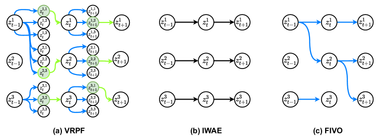
Figure 1: Comparison of VRPF with IWAE (Burda et al., 2015) and FIVO (Maddison et al., 2017) (a) The blue arrows represent the resampling step, We then generate multiple samples from parametrized proposal $z^{i}_{t}|z^{i}_{1:t-1}$ out of which one sample is accepted via PRC, depicted via green arrows. (b) In IWAE, there is no resampling step and no PRC step (c). In FIVO, there is a resampling step (blue arrows) but no PRC step.

When the variational distribution $q_{\phi}(.)$ is reparameterizable, we can make the sampling of $\delta^{i,k}_{t}$ independent of the model and variational parameters. However, the generated particles $z^{i}_{t}$ are not reparametrizable due to the PRC step. Finally, the ancestor variables are discrete and, therefore, cannot be reparameterized. The complete gradient can be divided into three core components (assuming $q_{\phi}(.)$ is reparametrizable)

$$\nabla_{\theta,\phi}\mathbb{E}[\hat{\mathcal{L}}_{\text{VRPF}}]=g_{\text{rep}}+g_{\text{PRC}}+g_{\text{RSAMP}},$$ (12)

$$g_{\text{rep}}=\mathbb{E}_{Q_{\text{VRPF}}}\left[\nabla_{\theta,\phi}\hat{\mathcal{L}}_{\text{VRPF}}\right],$$

$$g_{\text{PRC}}=\mathbb{E}_{Q_{\text{VRPF}}}\left[\hat{\mathcal{L}}_{\text{VRPF}}\nabla_{\theta,\phi}\sum_{i=1}^{N}\sum_{t=1}^{T}\log r_{\theta,\phi}(z^{i}_{t}|.)\right],$$

$$g_{\text{RSAMP}}=\mathbb{E}_{Q_{\text{VRPF}}}\left[\hat{\mathcal{L}}_{\text{VRPF}}\nabla_{\theta,\phi}\sum_{i=1}^{N}\sum_{t=1}^{T-1}A^{i}_{t}\log\alpha_{t}\right],$$

where $r_{\theta,\phi}(z^{i}_{t}|.)$ denotes the sampling density of the PRC step. Due to high gradient variance and intractability, we ignore $g_{\text{PRC}}$ and $g_{\text{RSAMP}}$ from the optimization. We have derived the full gradient and explored the gradient variance issues in the supplementary material. Please see Figure 2 (left) comparing the convergence of biased gradient vs. unbiased gradients on a toy Gaussian SSM.

3.3 Learning the M Matrix

We use $M$ as a hyperparameter for the PRC step which controls the acceptance rate of the sampler. The basic scheme of tuning $M$ is as follows:

• Define a new random variable $F\big{(}z_{t+1}|z_{1:t}^{A^{i}_{t}},x_{1:t+1}\big{)}=$

  $$\log\left(\frac{q_{\phi}\left(z_{t+1}|x_{1:t+1},z^{A^{i}_{t}}_{1:t}\right)}{p_{\theta}\left(x_{t+1},z_{t+1}|x_{1:t},z^{A^{i}_{t}}_{1:t}\right)}\right).$$

• For $j=1,2,\ldots,J$, draw

  $$z^{j}_{t+1}\sim q_{\phi}\left(z_{t+1}|x_{1:t+1},z^{A^{i}_{t}}_{1:t}\right)\,.$$

• Evaluate $\gamma\in[0,1]$ quantile value of $\{F(z^{j}_{t+1}|.)\}_{j=1}^{J}$. In general for this case the acceptance rate would be around $\gamma$ for all particles:

  $$\log M(i,t)=-\mathcal{Q}_{F(z_{t+1}|z_{1:t}^{A^{i}_{t}},x_{1:t+1})}(\gamma).$$ (13)

• If $M$ matrix is very large then use a common $\{M(.,t)\}_{t=1}^{T}$ for every time-step. In general, for this configuration, the acceptance rate would be greater than equal to $\gamma$ for all particles:

  $$\log M(.,t)=\min_{i=1,\dots,N}\left\{-\mathcal{Q}_{F(z_{t+1}|z_{1:t}^{A^{i}_{t}},x_{1:t+1})}(\gamma)\right\}.$$ (14)

Through $\gamma$: a user parameter, we can directly control the acceptance rate. Therefore, both Bernoulli race and PRC would take around (less than) $\gamma^{-1}$ iterations to produce a sample for $M$ value learned from (13) (see (14)). For implementation details please refer to the experiments. Algorithm 2 summarizes the complete optimization routine for the VRPF bound. We construct a stochastic gradient through (12) via a single draw from Algorithm 1. To save time, we will update $M$ once every $F$ epochs.

Algorithm 2 Optimization of VRPF lower bound

1:  Required: $p_{\theta}(x_{1:T},z_{1:T})$, $q_{\phi}(z_{1:T}|x_{1:T})$, $K$, $F$, $\gamma$

2:  Initialization: $M(i,t)=0\quad\forall i,t$ , $ep=0$

3:  while not converged  do

4:     Compute $g_{\text{rep}}$ via Eq. (12)

5:     $(\theta_{t+1},\phi_{t+1})=(\theta_{t},\phi_{t})+\eta_{t}g_{\text{rep}}(\theta_{t},\phi_{t})$

6:     $ep=ep+1$

7:     if  $ep\hskip 2.84526pt\text{mod}\hskip 2.84526ptF==0$  then

8:         Draw $\{z^{j}_{t+1}\}_{j=1}^{J}\sim q_{\phi}(z_{t+1}|x_{1:t+1},z^{A^{i}_{t}}_{1:t})\hskip 2.84526pt\forall i,t$

9:         Update $M(i,t)$ from Eq. (13)

10:     end if

11:  end while

12:  return $(\theta^{*},\phi^{*})$

4 Related Work and Special Cases

There is a significant recent interest in developing more expressive variational posteriors for LVM. One way to address this is by employing richer variational families i.e. using hierarchical models (Ranganath et al., 2016), copulas (Tran et al., 2015), or a sequence of invertible/non-invertible transformations (Rezende & Mohamed, 2015; Kumar et al., 2020). Another alternative, which is gaining attention lately is to combine VI with sampling methods. In particular,  Salimans et al. (2015); Domke (2017); Hoffman (2017); Li et al. (2017); Titsias (2017); Habib & Barber (2018); Zhang et al. (2018); Ruiz & Titsias (2019) use MCMC to construct a flexible VI bound. Other works uses approximate rejection sampling in a variational framework (Grover et al., 2018; Gummadi, 2014). Apart from flexible bounds, approximations of sampling-based methods have also been employed to improve the generated images through GAN (Goodfellow et al., 2014; Azadi et al., 2018; Turner et al., 2019; Neklyudov et al., 2018), construct richer priors for VAE (Bauer & Mnih, 2018), and improve gradient variance for VI (Naesseth et al., 2016).

The other direction is to construct a particle approximation within VI. Specifically, IWAE (Burda et al., 2015; Domke & Sheldon, 2018) uses importance sampling (IS) to construct tighter VI bounds. Although IS is useful in many scenarios, SMC can yield significantly better estimates for sequential settings (Doucet & Johansen, 2009). In particular Maddison et al. (2017); Naesseth et al. (2017); Le et al. (2017); Lawson et al. (2018) have shown that SMC yield superior results than IS within a variational framework for sequential data. For a detailed review on particle approximations in VI please refer to Domke & Sheldon (2019).

In this work, we present a unified framework for combining these two approaches, utilizing the best of both worlds. Although applying sampling-based methods on VI is useful, the density ratio between the true posterior and the improved density is often intractable. Therefore, we cannot take advantage of variance-reducing schemes like resampling, which is crucial for sequential models. We solve this issue through the Bernoulli race.

	$\mathbf{\log p_{\theta}(x_{1:T})}$	VSMC	$\mathbf{\gamma}=0.8$	$\mathbf{\gamma}=0.4$
Case 1	-18.27	-25.78	-24.80	-21.91
Case 2	-84.33	-230.46	-197.15	-187.25
Case 3	-33.89	-159.96	-108.47	-86.36
Case 4	-443.73	-538.33	-531.89	-515.10

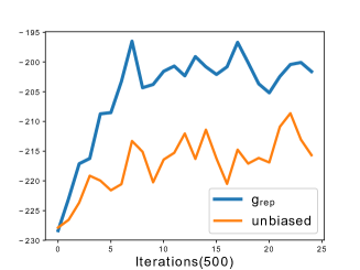
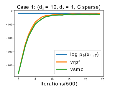
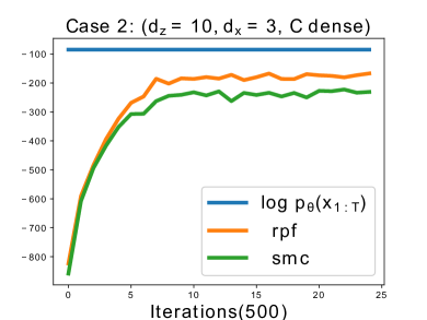
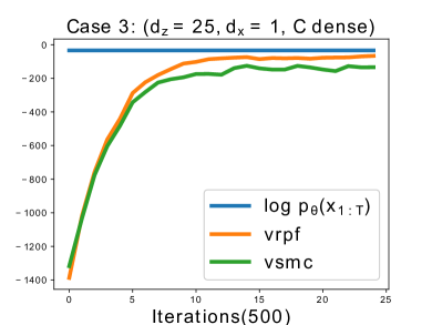
Figure 2: (Left) The figures compares the bound value for VRPF with full gradient and biased gradient ((12)) as a function of iterations. (Left) The Table compares the bound value for VSMC (Naesseth et al., 2017) and VRPF for $80\%$ and $40\%$ acceptance rate. (Right) We compare VSMC, VRPF ($40\%$ acceptance rate), and $\log p_{\theta}(x_{1:T})$ as a function of iterations.

Some closely related works to our method are VRS (Grover et al., 2018) and FIVO (Maddison et al., 2017). However, there are some key differences. In particular, consider a latent variable $\mathbf{z}_{1:t}=(z_{1},z_{2},\ldots,z_{t})$. In VRS, if the sample $\mathbf{z}^{i}_{1:t}$ is rejected, then we have to generate the entire sequence of intermediate $z_{j}$’s again, which could be costly for a large probabilistic system with long sequences. However, if a sample is rejected for our method, we generate a new sample from a parametrized proposal $z_{t}|z^{i}_{1:t-1}$; therefore, we only introduce a partial accept-reject at a local level, saving time. FIVO exploits the use of resampling within marginal likelihood estimation, thereby constructing a tight VI bound. However, in contrast to our method, it doesn’t exploit sampling-based methods like rejection sampling; therefore, VRPF tends to form a tighter VI bound than FIVO. We found that even introducing a partial accept-reject step with a high acceptance rate (more than 90 $\%$) is still useful. Please refer to Section 5.2 for more details.

A closely related work from SMC literature is BRPF (Schmon et al., 2019), which also utilizes Bernoulli factories to implement unbiased resampling. BRPF provides a general unbiased SMC construction when the true weights are intractable. However, unbiasedness though important is still not sufficient for formulating a VI bound; we also need efficient implementation along with improved performance. Unlike the existing BRPF frameworks which are limited to niche one-dimensional toy examples, the specific framework of VRPF is important for VI due to several reasons. First, it unifies sampling-based method with a particle approximation giving us a flexible family of VI bounds. Second, it belongs to the general family of BRPF; therefore one can use Bernoulli race to perform unbiased resampling. Finally, Section 3.3 demonstrates the efficient tuning of VRPF, thereby allowing us to scale our approach to general machine learning models like VRNN (Chung et al., 2015) in contrast to the current BRPF frameworks. Another relevant work for unbiased estimation of SMC with PRC is that of Kudlicka et al. (2020). In contrast to BRPF, this method samples one additional particle and keeps track of the number of steps required by PRC for every time-step to obtain their unbiased estimator. The weights are tractable for Kudlicka et al. (2020) as they do not take into account the effect of the normalization constant $Z(.)$. It is important to note however that Kudlicka et al. (2020) does not consider the exact setting of Peters et al. (2012). Therefore, one cannot use Kudlicka et al. (2020) directly for VRPF in contrast to BRPF.

To provide more clarity, we will consider some special cases of VRPF bound and relate it with existing work: Note that for $N=1$ our method reduces to a special case of Gummadi (2014) which uses a constraint function $C_{t}$ for every time-step and restarts the particle trajectory from $\Delta_{t}$ (if $C_{t}$ is violated). Therefore, if we use the setting $C_{t}(z_{1:t})=a(z_{t}|z_{1:t-1},x_{1:t})$ and $\Delta_{t}=t-1$, we recover a particular case of Gummadi (2014). For the special case of $N=1$ and $T=1$, our method reduces to VRS (Grover et al., 2018). For $N,T>1$, if we remove the PRC step, our bound reduces to FIVO (Maddison et al., 2017). Finally, if we remove both the PRC step and resampling, then our method effectively reduces to IWAE (Burda et al., 2015). Please refer to Figure 1 for more details.

5 Experiments

We evaluate our proposed algorithm on synthetic as well as real-world datasets and compare them with relevant baselines. For the synthetic data experiment, we implement our method on a Gaussian SSM and compare with VSMC (Naesseth et al., 2017). For the real data experiment, we train a VRNN (Chung et al., 2015) on the polyphonic music dataset.

5.1 Gaussian State Space Model

In this experiment, we study the linear Gaussian state space model. Consider the following setting

$$z_{t}=Az_{t-1}+e_{z},$$

$$x_{t}=Cz_{t}+e_{x},$$

where $e_{z},e_{x}\sim\mathcal{N}(0,I)$ and $z_{0}=0$. We are interested in learning a good proposal for the above model. The latent variable is denoted by $z_{t}$ and the observed data by $x_{t}$. Let the dimension of $z_{t}$ be $d_{z}$ and dimension of $x_{t}$ be $d_{x}$. The matrix $A$ has the elements $(A)_{i,j}=\alpha^{|i-j|+1}$, for $\alpha=0.42$.

We explore different settings of $d_{z},d_{x}$, and matrix $C$. A sparse version of $C$ matrix measures the first $d_{x}$ components of $z_{t}$, on the other hand a dense version of $C$ is normally distributed i.e $C_{i,j}\sim\mathcal{N}(0,1)$. We consider four different configurations for the experiment. For more details please refer to Figure (2).

The variational distribution is a multivariate Gaussian with unknown mean vector $\mu=\{\mu_{d}\}_{d=1}^{d_{z}}$ and diagonal covariance matrix $\{\log\sigma_{d}^{2}\}_{d=1}^{d_{z}}$. We set $N=4$ and $T=10$ for all the cases:

$$q(z_{t}|z_{t-1})\sim\mathcal{N}\left(z_{t}|Az_{t-1}+\mu,\text{diag}(\sigma^{2})\right).$$

The $M$ matrix (see Eq. (13)) for approximate rejection sampling is updated once every $F=10$ epochs with acceptance rate $\gamma\in\{0.8,0.4\}$. For estimating the intractable normalization constants, we set $K=3$. Figure 2: (left) compares the convergence of biased gradient vs unbiased gradients. Note that we obtain a much tighter bound as compared to VSMC (Naesseth et al., 2017).

5.2 Variational RNN

VRNN (Chung et al., 2015) comprises of three core components: the observation $x_{t}$, stochastic latent state $z_{t}$, and a deterministic hidden state $h_{t}(z_{t-1},x_{t-1},h_{t-1})$, which is modeled through a RNN. For the experiments, we use a single-layer LSTM for modeling the hidden state. The conditional distributions $p_{t}(z_{t}|.)$ and $q_{t}(z_{t}|.)$ are assumed to be factorized Gaussians, parametrized by a single layer neural net. The output distribution $g_{t}(x_{t}|.)$ depends on the dataset. For a fair comparison, we use the same model setting as employed in FIVO (Maddison et al., 2017). We evaluate our model on four polyphonic music datasets: Nottingham, JSB chorales, Musedata, and Piano-midi.de (Boulanger-Lewandowski et al., 2012).

Table 1: We report Test log-likelihood for models trained with FIVO, IWAE, ELBO, and VRPF. For VRPF $N=(4,6)$ and $(K,\gamma)\in\{(1,0.9),(1,0.8),(3,0.9),(3,0.8)\}$ (results are in this order). The results for pianoroll data-sets are in nats per timestep.

N	Data	ELBO	IWAE	FIVO	N	VRPF
	Nott	-3.87	-3.12	-3.07		-2.96	-2.98	-2.99	-2.96
	jsb	-8.69	-8.01	-7.51		-7.41	-7.28	-7.37	-7.36
5	Piano	-7.99	-7.97	-7.85	4	-7.82	-7.86	-7.80	-7.85
	Muse	-7.48	-7.45	-6.75		-6.61	-6.63	-6.66	-6.58
N	Data	ELBO	IWAE	FIVO	N	VRPF
	Nott	-3.87	-3.87	-2.99		-2.93	-2.93	-2.90	-2.91
	jsb	-8.69	-8.32	-7.40		-7.29	-7.21	-7.16	-7.14
8	Piano	-7.99	-8.04	-7.80	6	-7.78	-7.77	-7.79	-7.77
	Muse	-7.48	-7.41	-6.67		-6.60	-6.57	-6.61	-6.60
Avg. Rank		6.87 $\pm$ 0.33	6.12 $\pm$ 0.33	4.87 $\pm$ 0.33		2.87 $\pm$ 1.05	2.62 $\pm$ 1.21	2.87 $\pm$ 1.26	1.75 $\pm$ 0.66

Each observation $x_{t}$ is represented as a binary vector of 88 dimensions. Therefore, we model the observation distribution $g_{t}(x_{t}|.)$ by a set of 88 factorized Bernoulli variables. We split all four data-sets into the standard train, validation, and test sets. For tuning the learning rate, we use the validation test set. Let the dimension of hidden state (learned by single layer LSTM) be $d_{h}$ and dimension of latent variable be $d_{z}$. We choose the setting $d_{z}=d_{h}=64$ for all the data-sets except JSB. For modeling JSB, we use $d_{z}=d_{h}=32$. For VRPF we have considered $N\in\{4,6\}$ Further, for every $N$, we consider four settings $(K,\gamma)\in\{(1,0.9),(1,0.8),(3,0.9),(3,0.8)\}$. The $M$ hyper-parameter for the PRC step is learned from Eq. (14) due to large size and is updated once every $F=50$ epochs. Note that in this scenario, the acceptance rate for all particles would be greater than equal to $\gamma$. For more details on experiments, please refer to the supplementary material.

As discussed in Section (3.1), the PRC step and Bernoulli race have time complexity $\mathcal{O}(N/\gamma)$ for producing $N$ samples (assuming average acceptance rate $\gamma$). Therefore, we consider $\lceil N\gamma^{-1}\rceil$ particles for IWAE and FIVO to ensure effectively the same number of particles, where $N\in\{4,6\}$ and $\gamma=0.8$. Note, however, that the acceptance rate is $\geq\gamma$, so this adjustment actually favors the other approaches more. For FIVO, we perform resampling when ESS falls below $N/2$. Table 1 summarizes the results which show whether rejecting samples provide us with any benefit or not, and as the results show, our approach, even with the aforementioned adjustment, outperforms the other approaches in terms of test log-likelihoods.

In VRPF, improvement in the bound value comes at the cost of estimating the normalization constant $Z(.)$, i.e., $K$. On further inspection, we can clearly see that increasing $K$ doesn’t provide us with any substantial benefits despite the increase in computational cost. Therefore, to maintain the computational trade-off $(K=1,\gamma>0.8)$ seems to be a reasonable choice for VI practitioners.

Table 1 signifies that rejecting samples with low importance weight is better instead of keeping a large number of particles (at least for a reasonably high acceptance rate $\gamma$). It is interesting to note that partial accept-reject indeed helps empirically. In the above VRNN experiment the latent variable $\mathbf{z}_{1:T}$ is fairly high-dimensional for example: in Piano-midi.de the maximum sequence length is of order $10^{6}$. Therefore, it is straightforward to verify that one cannot use sampling-based methods directly.

Our experimental results indicate that partial sampling is useful even for high-dimensional applications. Specifically, we want to emphasize that accept-reject though useful, is still limited in its nature compared to MCMC algorithms like Hamiltonian Monte Carlo (HMC) (Neal et al., 2011). Note, however, we are still getting improved results for such large sequences despite using accept-reject. Therefore, exploring the general area of partial/greedy sampling within high-dimensional time series models would make for interesting future work.

6 Conclusion

We introduced VRPF, a novel bound that combines SMC and partial rejection sampling with VI in a synergistic manner. This results in a robust VI procedure for sequential latent variable models. Instead of using standard sampling algorithms, we have employed a partial sampling scheme suitable for high dimensional sequences. Our experimental results clearly demonstrate that VRPF outperforms existing bounds like IWAE (Burda et al., 2015) and standard particle filter bounds (Maddison et al., 2017; Naesseth et al., 2017; Le et al., 2017). Future work aims at designing a scalable implementation for VRPF bound that consumes fewer particles and exploring partial versions of powerful sampling algorithms like HMC instead of rejection sampling.

References

- Asmussen et al. (1992) Asmussen, S., Glynn, P. W., and Thorisson, H. Stationarity detection in the initial transient problem. ACM Transactions on Modeling and Computer Simulation (TOMACS), 2(2):130–157, 1992.
- Azadi et al. (2018) Azadi, S., Olsson, C., Darrell, T., Goodfellow, I., and Odena, A. Discriminator rejection sampling. arXiv preprint arXiv:1810.06758, 2018.
- Bauer & Mnih (2018) Bauer, M. and Mnih, A. Resampled priors for variational autoencoders. arXiv preprint arXiv:1810.11428, 2018.
- Bérard et al. (2014) Bérard, J., Del Moral, P., Doucet, A., et al. A lognormal central limit theorem for particle approximations of normalizing constants. Electronic Journal of Probability, 19, 2014.
- Blei et al. (2017) Blei, D. M., Kucukelbir, A., and McAuliffe, J. D. Variational inference: A review for statisticians. Journal of the American Statistical Association, 112(518):859–877, 2017.
- Boulanger-Lewandowski et al. (2012) Boulanger-Lewandowski, N., Bengio, Y., and Vincent, P. Modeling temporal dependencies in high-dimensional sequences: Application to polyphonic music generation and transcription. arXiv preprint arXiv:1206.6392, 2012.
- Burda et al. (2015) Burda, Y., Grosse, R., and Salakhutdinov, R. Importance weighted autoencoders. arXiv preprint arXiv:1509.00519, 2015.
- Chung et al. (2015) Chung, J., Kastner, K., Dinh, L., Goel, K., Courville, A. C., and Bengio, Y. A recurrent latent variable model for sequential data. In Advances in neural information processing systems, pp. 2980–2988, 2015.
- Domke (2017) Domke, J. A divergence bound for hybrids of mcmc and variational inference and an application to langevin dynamics and sgvi. In International Conference on Machine Learning, pp. 1029–1038. PMLR, 2017.
- Domke & Sheldon (2018) Domke, J. and Sheldon, D. Importance weighting and variational inference. arXiv preprint arXiv:1808.09034, 2018.
- Domke & Sheldon (2019) Domke, J. and Sheldon, D. Divide and couple: Using monte carlo variational objectives for posterior approximation. arXiv preprint arXiv:1906.10115, 2019.
- Doucet & Johansen (2009) Doucet, A. and Johansen, A. M. A tutorial on particle filtering and smoothing: Fifteen years later. Handbook of nonlinear filtering, 12(656-704):3, 2009.
- Dughmi et al. (2017) Dughmi, S., Hartline, J. D., Kleinberg, R., and Niazadeh, R. Bernoulli factories and black-box reductions in mechanism design. In Proceedings of the 49th Annual ACM SIGACT Symposium on Theory of Computing, pp. 158–169, 2017.
- Goodfellow et al. (2014) Goodfellow, I., Pouget-Abadie, J., Mirza, M., Xu, B., Warde-Farley, D., Ozair, S., Courville, A., and Bengio, Y. Generative adversarial nets. In Advances in neural information processing systems, pp. 2672–2680, 2014.
- Grover et al. (2018) Grover, A., Gummadi, R., Lazaro-Gredilla, M., Schuurmans, D., and Ermon, S. Variational rejection sampling. arXiv preprint arXiv:1804.01712, 2018.
- Gummadi (2014) Gummadi, R. Resampled belief networks for variational inference. In NIPS Workshop on Advances in Variational Inference, 2014.
- Habib & Barber (2018) Habib, R. and Barber, D. Auxiliary variational mcmc. In International Conference on Learning Representations, 2018.
- Hoffman (2017) Hoffman, M. D. Learning deep latent Gaussian models with Markov chain Monte Carlo. In Proceedings of the 34th International Conference on Machine Learning-Volume 70, pp. 1510–1519. JMLR. org, 2017.
- Hoffman et al. (2013) Hoffman, M. D., Blei, D. M., Wang, C., and Paisley, J. Stochastic variational inference. Journal of Machine Learning Research, 14(5), 2013.
- Kingma & Welling (2013) Kingma, D. P. and Welling, M. Auto-encoding variational bayes. arXiv preprint arXiv:1312.6114, 2013.
- Kudlicka et al. (2020) Kudlicka, J., Murray, L. M., Schön, T. B., and Lindsten, F. Particle filter with rejection control and unbiased estimator of the marginal likelihood. In ICASSP 2020-2020 IEEE International Conference on Acoustics, Speech and Signal Processing (ICASSP), pp. 5860–5864. IEEE, 2020.
- Kumar et al. (2020) Kumar, A., Poole, B., and Murphy, K. Regularized autoencoders via relaxed injective probability flow. In International Conference on Artificial Intelligence and Statistics, pp. 4292–4301. PMLR, 2020.
- Lawson et al. (2018) Lawson, D., Tucker, G., Naesseth, C. A., Maddison, C. J., Adams, R. P., and Teh, Y. W. Twisted variational sequential Monte Carlo. In Third workshop on Bayesian Deep Learning (NeurIPS), 2018.
- Le et al. (2017) Le, T. A., Igl, M., Rainforth, T., Jin, T., and Wood, F. Auto-encoding sequential Monte Carlo. arXiv preprint arXiv:1705.10306, 2017.
- Li et al. (2017) Li, Y., Turner, R. E., and Liu, Q. Approximate inference with amortised MCMC. arXiv preprint arXiv:1702.08343, 2017.
- Liu et al. (1998) Liu, J. S., Chen, R., and Wong, W. H. Rejection control and sequential importance sampling. Journal of the American Statistical Association, 93(443):1022–1031, 1998.
- Maddison et al. (2017) Maddison, C. J., Lawson, J., Tucker, G., Heess, N., Norouzi, M., Mnih, A., Doucet, A., and Teh, Y. Filtering variational objectives. In Advances in Neural Information Processing Systems, pp. 6573–6583, 2017.
- Naesseth et al. (2016) Naesseth, C. A., Ruiz, F. J., Linderman, S. W., and Blei, D. M. Reparameterization gradients through acceptance-rejection sampling algorithms. arXiv preprint arXiv:1610.05683, 2016.
- Naesseth et al. (2017) Naesseth, C. A., Linderman, S. W., Ranganath, R., and Blei, D. M. Variational sequential Monte Carlo. arXiv preprint arXiv:1705.11140, 2017.
- Neal et al. (2011) Neal, R. M. et al. MCMC using Hamiltonian dynamics. Handbook of markov chain monte carlo, 2(11):2, 2011.
- Neklyudov et al. (2018) Neklyudov, K., Egorov, E., Shvechikov, P., and Vetrov, D. Metropolis-hastings view on variational inference and adversarial training. arXiv preprint arXiv:1810.07151, 2018.
- Peters et al. (2012) Peters, G. W., Fan, Y., and Sisson, S. A. On sequential Monte Carlo, partial rejection control and approximate Bayesian computation. Statistics and Computing, 22(6):1209–1222, 2012.
- Ranganath et al. (2014) Ranganath, R., Gerrish, S., and Blei, D. Black box variational inference. In Artificial Intelligence and Statistics, pp. 814–822, 2014.
- Ranganath et al. (2016) Ranganath, R., Tran, D., and Blei, D. Hierarchical variational models. In International Conference on Machine Learning, pp. 324–333, 2016.
- Rezende & Mohamed (2015) Rezende, D. J. and Mohamed, S. Variational inference with normalizing flows. arXiv preprint arXiv:1505.05770, 2015.
- Robert & Casella (2013) Robert, C. and Casella, G. Monte Carlo statistical methods. Springer Science & Business Media, 2013.
- Ruiz & Titsias (2019) Ruiz, F. J. and Titsias, M. K. A contrastive divergence for combining variational inference and MCMC. arXiv preprint arXiv:1905.04062, 2019.
- Salimans et al. (2015) Salimans, T., Kingma, D., and Welling, M. Markov chain Monte Carlo and variational inference: Bridging the gap. In International Conference on Machine Learning, pp. 1218–1226, 2015.
- Schmon et al. (2019) Schmon, S. M., Doucet, A., and Deligiannidis, G. Bernoulli race particle filters. arXiv preprint arXiv:1903.00939, 2019.
- Titsias (2017) Titsias, M. K. Learning model reparametrizations: Implicit variational inference by fitting MCMC distributions. arXiv preprint arXiv:1708.01529, 2017.
- Tran et al. (2015) Tran, D., Blei, D., and Airoldi, E. M. Copula variational inference. In Advances in Neural Information Processing Systems, pp. 3564–3572, 2015.
- Turner et al. (2019) Turner, R., Hung, J., Frank, E., Saatchi, Y., and Yosinski, J. Metropolis-hastings generative adversarial networks. In International Conference on Machine Learning, pp. 6345–6353. PMLR, 2019.
- Zhang et al. (2018) Zhang, Y., Hernández-Lobato, J. M., and Ghahramani, Z. Ergodic measure preserving flows. arXiv preprint arXiv:1805.10377, 2018.