Higher order cumulants of transverse momentum and harmonic flow in relativistic heavy ion collisions

Abstract

Higher order symmetric cumulants of global collective observables in heavy ion collisions are studied. The symmetric cumulants can be straightforwardly constructed for scalar observables : the average transverse momentum, the multiplicity, and the squares of harmonic flow vectors. Third and fourth order cumulants are calculated in the hydrodynamic model. A linear predictor of the average transverse momentum and harmonic flow coefficients in a collision is used to predict the value of the cumulants from the moments of the initial distribution. The symmetric cumulants divided by the averages (or the standard deviations) of the considered observables can be used as a fine tool to study correlations present in the initial state of the collision.

I Introduction

The dense matter created in relativistic heavy ion collisions expands rapidly. The study of the collective flow of the expanding matter, modeled by the viscous hydrodynamics, can be used to study its properties Ollitrault:2010tn ; Heinz:2013th ; Gale:2013da . One of the difficulties in this tasks lies in the uncertainty on the initial conditions for the hydrodynamic evolution. To reduce the uncertainty in the prediction of the harmonic flow coefficients, a number of additional observables based on correlators involving four or more particles have been proposed to constrain the initial conditions.

The expansion in the directions transverse to the beam direction generates the collective transverse flow. Of particular importance are the harmonic coefficients of the azimuthal particle distribution reflecting the azimuthal asymmetry of the initial conditions. The average transverse momentum of particles emitted in a collision is a measure of the overall radial expansion. The final transverse momentum is related to the size of the initial source Broniowski:2009fm . Events with a smaller size of the interaction region have larger energy density gradients and a larger transverse push is formed in the expansion. The scaled transverse momentum fluctuations reflect, in the first approximation, the fluctuations of the initial size and in the entropy deposition.

A finer tool to look at the correlations of the collective flow observables in heavy ion collisions is given by the correlation coefficient $\rho(p_{T},v_{n}^{2})$ between the average transverse momentum $p_{T}$ and the harmonic flow coefficient $v_{n}^{2}$ in an event Bozek:2016yoj . The correlation of the elliptic or triangular flow with the average transverse momentum is well described by the correlations present in the initial state of the hydrodynamic evolution Bozek:2020drh ; Schenke:2020uqq ; Giacalone:2020dln . Thus, the correlation coefficient of transverse momentum $p_{T}$ and the elliptic or triangular flow coefficient can serve as a tool to study correlations present in the initial state. The correlation coefficient has been measured for Pb+Pb and p+Pb collisions by the ATLAS Collaboration Aad:2019fgl . The experimental data on $\rho([p_{T}],v_{2}^{2})$ in Pb+Pb collisions are qualitatively well described by hydrodynamic models. On the other hand, the magnitude and the sign of the correlation coefficient $\rho([p_{T}],v_{3}^{2})$ are not well described in most of the calculations.

The study of the correlation coefficient between transverse momentum and elliptic flow is particularly interesting in deformed nuclei. In central collisions of deformed nuclei the orientation of the colliding deformed nuclei leads to specific correlations between the initial size and the elliptic deformation Giacalone:2019pca ; Giacalone:2020awm . Experimental results show a sensitivity of the correlation coefficient $\rho([p_{T}],v_{2}^{2})$ to the nuclear deformation ATLAS:2021kty ; JiaIS2021 . The transverse momentum-harmonic flow correlation coefficient in peripheral events can be sensitive to initial momentum correlation that would survive the hydrodynamic evolution Giacalone:2020byk .

In this paper we explore higher order correlators of the harmonic flow and of the average transverse momentum. We study higher order symmetric cumulants Bilandzic:2013kga ; Mordasini:2019hut ; Moravcova:2020wnf of scalar quantities: the transverse momentum, multiplicity, and the squares of harmonic flow vectors of different order. We present predictions for the third and four order normalized symmetric cumulants for collisions of spherical Pb+Pb and deformed U+U nuclei in the hydrodynamic model. We propose two different ways to normalize the higher cumulants, by the average or by the standard deviations of the observables taken in the cumulant. The calculations are compared to the results obtained using a linear predictor based on moments of the initial density. The higher order cumulants calculated in the hydrodynamic model could be measured experimentally.

II Correlations of global observables in an event

II.1 Model

Expanding the azimuthal dependence of particle distributions in Fourier series we can write

$$\frac{dN}{dpd\phi}=\frac{dN}{2\pi dp}\left(1+2\sum_{n=1}^{\infty}V_{n}(p)e^{in\phi}\right)\ ,$$ (1)

using the complex plane notation for the transverse plane ($p$,$\phi$). In this paper we use boost invariant calculations and the results should be compared to experimental results obtained at central rapidities in heavy-ion collisions. Both the transverse momentum distribution $\frac{dN}{dp}$ and the harmonic flow vectors $V_{n}$ fluctuate event by event. In this paper we study event by event correlations between moments of the distribution $\frac{dN}{dpd\phi}$ integrated in a range of transverse momenta, the charged particle multiplicity

$$N=\int_{p_{min}}^{p_{max}}dp\frac{dN}{dp}$$ (2)

the average transverse momentum in an event

$$p_{T}=\frac{1}{N}\int_{p_{min}}^{p_{max}}pdp\frac{dN}{dp}$$ (3)

and the harmonic flow coefficients

$$V_{n}=\frac{1}{N}\int_{p_{min}}^{p_{max}}dpV_{n}(p)\frac{dN}{dp}.$$ (4)

The complex numbers $V_{n}=v_{n}e^{in\Psi_{n}}$ describe the flow magnitude $v_{n}$ and the flow angle $\Psi_{n}$ for the harmonic flow of order $n$. The average over a sample of events in a given centrality bin is denoted by $\langle\dots\rangle$, e.g. the averages of the multiplicity $\langle N\rangle$ , transverse momentum $\langle p_{T}\rangle$, and flow harmonics

$$v_{n}\{2\}=\sqrt{\langle V_{n}V_{n}^{\star}\rangle}$$ (5)

can be calculated.

We use the 2-dimensional version of the hydrodynamic code MUSIC Schenke:2010nt ; Schenke:2010rr ; Paquet:2015lta with shear viscosity $\eta/s=0.08$ for the hydrodynamic expansion phase. For the initial conditions in Pb+Pb collisions at $\sqrt{s_{NN}}=5.02$ TeV we use a two-component Glauber Monte Carlo model Bozek:2019wyr to calculate the initial entropy density in each event. The details of the model for the initial density can be found in Bozek:2016yoj . The initial density in the transverse plane $s(x,y)$ in each event can be characterized by specific moments, the eccentricities

$$\epsilon_{n}e^{i\Phi_{n}}=-\frac{\int rdrd\phi\ r^{n}s(r,\phi)e^{in\phi}}{\int rdrd\phi\ r^{n}s(r,\phi)}\ ,$$ (6)

the RMS radius

$$R^{2}=\frac{\int rdrd\phi\ r^{2}s(r,\phi)}{\int rdrd\phi\ s(r,\phi)}\ ,$$ (7)

and the entropy per unit rapidity

$$S=\int rdrd\phi\ s(r,\phi)\ .$$ (8)

II.2 Transverse momentum - harmonic flow correlations

Event by event correlations between the average transverse momentum and the harmonic flow can be measured using the correlation coefficient Bozek:2016yoj

$$\rho(p_{T},v_{n}^{2})=\frac{Cov(p_{T},v_{n}^{2})}{\sqrt{Var(p_{T})Var(v_{n}^{2})}}$$ (9)

with the covariance

$$Cov(p_{T},v_{n}^{2})=\langle p_{T}V_{n}V_{n}^{\star}\rangle-\langle p_{T}\rangle\langle V_{n}V_{n}^{\star}\rangle$$ (10)

and the variances

$$Var(p_{T})=\langle p_{T}^{2}\rangle-\langle p_{T}\rangle^{2}\ ,$$ (11)

$$Var(v_{n}^{2})=\langle(V_{n}V_{n}^{\star})^{2}\rangle-\langle V_{n}V_{n}^{\star}\rangle^{2}.$$ (12)

The covariance in the numerator of the correlation coefficient (9) is a three particle correlators, but the variance of the flow harmonic (12) is a four particle correlator. The experimental estimators for covariance and the variances in (9) involve up to three or four sums over particles in the event, with self-correlations excluded Bozek:2016yoj

Figure 1: The correlation coefficient of the average transverse momentum and the elliptic flow coefficient in Pb+Pb collisions as a function of centrality. The experimental data are from the ATLAS Collaboration ATLAS:2021kty (blue points). The red squares denote the results of the hydrodynamic simulations, the black triangles show the results for the correlation coefficient corrected for multiplicity fluctuations (13) and the blue dashed line with stars shows the correlation coefficient obtained from the linear predictor (15).

Figure 2: Same as in Fig. 1, but for the triangular flow.

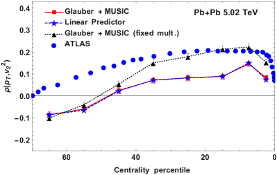
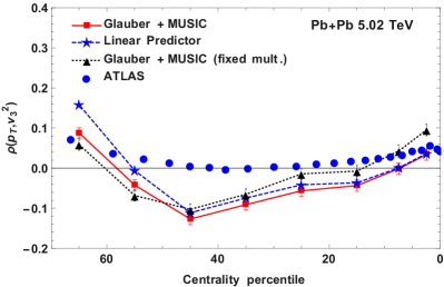
The results for the transverse momentum-elliptic flow correlation coefficient $\rho(p_{T},v_{2}^{2})$ are shown in Fig. 1. The simulated correlation coefficients are qualitatively similar to the experimental data of the ATLAS Collaboration ATLAS:2021kty . In particular, the correlation coefficient $\rho(p_{T},v_{2}^{2})$ decreases in the most central collisions, and in peripheral collisions the correlation coefficient changes sign. The measured correlation coefficient for the triangular flow $\rho(p_{T},v_{3}^{2})$ is small and is shown in Fig.2. The simulation does not fully describe this feature of the experimental data.

The correlation between the average transverse momentum and the flow harmonics is partially due to correlations of those quantities with the event multiplicity. The experimental data is presented in narrow bins of centrality, where this effect is reduced. The dependence of the variance or covariance of studied observables on the fluctuations of a third variable, e.g. the multiplicity, can be taken into account by calculating the partial variance or covariance Olszewski:2017vyg . The partial correlation coefficient

$$\rho(p_{T},v_{n}^{2}\bullet N)=\frac{\rho(p_{T},v_{n}^{2})-\rho(p_{T},N)\rho(N,v_{n}^{2})}{\sqrt{1-\rho(p_{T},N)^{2}}\sqrt{1-\rho(v_{n}^{2},N)^{2}}}$$ (13)

is an estimate of the correlation coefficient at fixed multiplicity Bozek:2019wyr . The results for the partial correlation coefficients are shown in Figs. 1 and 2 (black triangles). The correction is sizable for the elliptic flow correlations coefficient $\rho(p_{T},v_{2}^{2})$. The partial correlation coefficient is closer to the experimental data. Generally, if the dependence of an observable $O$, in a given bin, on multiplicity is approximately linear, the correction to $O$ can be implemented as Schenke:2020uqq

$$\tilde{O}=O-\frac{Cov(O,N)}{Var(N)}\left(N-\langle N\rangle\right)$$ (14)

To correct for the effect of multiplicity fluctuation, we can calculate event averages for moments of the corrected variables (14). For the correlation coefficient this procedure is equivalent to the formula for the partial correlation coefficient (13). In the following, we use the corrected observables $\tilde{O}$ to estimate higher order cumulants without effects of multiplicity fluctuations.

II.3 Linear predictor

The average transverse momentum and the harmonic flow coefficients are largely determined by the initial conditions Gardim:2011xv ; Qiu:2011iv ; Niemi:2012aj ; Broniowski:2009fm . The eccentricities of the initial distribution are strongly correlated with harmonic flow coefficients of the emitted particles. The average transverse momentum of final particles can be predicted using the initial entropy $S$ (8) and the RMS size $R$ (7) Mazeliauskas:2015efa ; Bozek:2017elk . Alternatively, a predictor of the final transverse momentum based on the initial energy per rapidity can be used Giacalone:2020dln or the energy weighted entropy Schenke:2020uqq .

It has been noted, that in order to describe the correlation of the transverse momentum with the elliptic or triangular flow, the eccentricities should be included in the predictor for the final transverse moments Bozek:2020drh . It was shown that such an improved predictor describes well the transverse momentum-harmonic flow correlations coefficient obtained from the full hydrodynamic simulation. In the following we use a general linear predictor, based on moments of the initial density

$$\hat{v}_{2}^{2} = k_{2}\epsilon_{2}^{2}+\alpha_{2}\delta R+\beta_{2}\delta S$$

$$\hat{v}_{3}^{2} = k_{3}\epsilon_{3}^{2}+\alpha_{3}\delta R+\beta_{3}\delta S$$

$$\hat{p}_{T} = \langle p_{T}\rangle+\alpha_{p}\delta R+\beta_{p}\delta S+\gamma_{p}\delta\epsilon^{2}+\lambda_{p}\delta\epsilon_{3}^{2}\ \ \ ,$$ (15)

where for any observable $\delta O=O-\langle O\rangle$. The prediction of each of the observables in the above equations is optimized separately. Only after fixing the parameters of the linear predictor, the cumulants between predicted observables are calculated. The linear predictor can be written as

$$\delta\hat{O}_{i}=L^{j}_{i}\delta M_{j}$$ (16)

with $M_{i}$ being the set of moments of the initial density. The moments of the final observables can be written as a linear transformation from the moments in the initial state

$$\langle\delta O_{i}\dots\delta O_{j}\rangle=L^{s}_{i}\dots L^{k}_{j}\langle\delta M_{s}\dots\delta M_{k}\rangle\ .$$ (17)

The linear predictor (15) describes fairly well the correlations and higher cumulants involving $p_{T}$, $v_{2}^{2}$, and $v_{3}^{2}$. It demonstrates that the proposed cumulants involving those observables can be understood as a linear hydrodynamic response on the correlations present in the initial state.

III Symmetric cumulants

III.1 Second order cumulant

The correlation between the magnitudes of the harmonic flows of different order has been studied using symmetric cumulants Bilandzic:2013kga . The second order symmetric cumulant is the covariance between the two observables

$$\langle AB\rangle-\langle A\rangle\langle B\rangle=Cov(A,B)\ .$$ (18)

The normalized symmetric cumulant is scaled by the averages of the observables in the covariance. For the transverse momentum and harmonic flow one may define

$$NSC(p_{T},v_{n}^{2})=\frac{\langle p_{T}v_{n}^{2}\rangle-\langle p_{T}\rangle\langle v_{n}^{2}\rangle}{\langle p_{T}\rangle\langle v_{n}^{2}\rangle}\ .$$ (19)

Figure 3: The normalized symmetric cumulant of the average transverse momentum and of the elliptic flow coefficient in Pb+Pb collisions as a function of centrality. The red squares denote the results of the hydrodynamic simulations, the black triangles show the results for the cumulant obtained for observable corrected for multiplicity fluctuations (14) and the blue dashed line shows the correlation coefficient obtained from the linear predictor (15).

Figure 4: Same as in Fig. 3, but for the triangular flow.

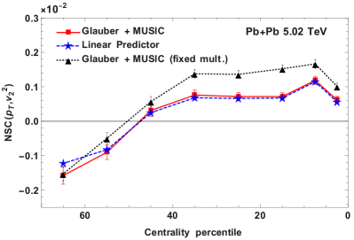
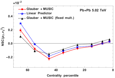
For completeness, the normalized symmetric cumulants for transverse momentum and harmonic flow are shown in Figs. 3 and 4. The information on the event by event correlations between the average transverse momentum and the harmonic flow is contained in the covariance of the two observable, and is basically the same in the correlation coefficient $\rho(p_{T},v_{n}^{2})$ and in the symmetric cumulant $NSC(p_{T},v_{n}^{2})$. The experimental extraction of the normalized symmetric cumulants is simpler than for the correlation coefficient, since the denominator involves at most a two particle correlator, where methods to reduce non-flow effects can be implemented, even in small collision systems Zhang:2021phk .

IV Third and fourth order cumulants

Additional information on correlations between flow observables is encoded in higher order cumulants Bilandzic:2013kga ; Mordasini:2019hut ; Moravcova:2020wnf . The $n$-th order cumulant involves only correlation of $n$ observables, with all lower order correlations subtracted. The third and fourth order symmetric cumulants for scalar observables have the form Mordasini:2019hut

$$SC(A,B,C) = \langle ABC\rangle-\langle AB\rangle\langle C\rangle-\langle AC\rangle\langle B\rangle$$ (20)

$$-\langle BC\rangle\langle A\rangle+2\langle A\rangle\langle B\rangle\langle C\rangle$$

and

$$SC(A,B,C,D) = \langle ABCD\rangle-\langle ABC\rangle\langle D\rangle-\langle ABD\rangle\langle C\rangle$$ (21)

$$-\langle ACD\rangle\langle B\rangle-\langle BCD\rangle\langle A\rangle-\langle AB\rangle\langle CD\rangle$$

$$-\langle AC\rangle\langle BD\rangle-\langle BC\rangle\langle AD\rangle$$

$$+2\left(\langle AB\rangle\langle C\rangle\langle D\rangle+\langle AC\rangle\langle B\rangle\langle D\rangle\right.$$

$$+\langle AD\rangle\langle C\rangle\langle B\rangle+\langle BC\rangle\langle A\rangle\langle D\rangle$$

$$\left.+\langle BD\rangle\langle A\rangle\langle C\rangle+\langle CD\rangle\langle A\rangle\langle B\rangle\right)$$

$$-6\langle A\rangle\langle B\rangle\langle C\rangle\langle D\rangle$$

The corresponding normalized symmetric cumulants are

$$NSC(A,B,C)=\frac{SC(A,B,C)}{\langle A\rangle\langle B\rangle\langle C\rangle}$$ (22)

and

$$NSC(A,B,C,D)=\frac{SC(A,B,C,D)}{\langle A\rangle\langle B\rangle\langle C\rangle\langle D\rangle}$$ (23)

As noted, for higher order symmetric cumulants the effect of multiplicity fluctuations can be reduced using observables corrected for changes in multiplicity (14).

Figure 5: The normalized symmetric cumulant of the average transverse momentum and the squares of the elliptic and triangular flow (red squares). The blue stars denote the results obtained from the linear predictor (15) and the black triangles show the scaled symmetric cumulant for observables corrected for multiplicity fluctuations (14).

Figure 6: Same as in Fig. 5 but for the triangular and quadratic flows.

Figure 7: Same as in Fig. 5 but for the elliptic and quadratic flows.

Figure 8: The fourth order normalized symmetric cumulant between the average transverse momentum and the harmonic flow of orders 2, 3, and 4 for Pb+Pb collisions at $\sqrt{s_{NN}}=5.02$ TeV, as a function of centrality (red squares). The black triangles denote the corresponding results for observable corrected for multiplicity fluctuations (14).

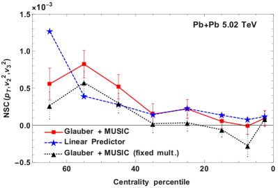
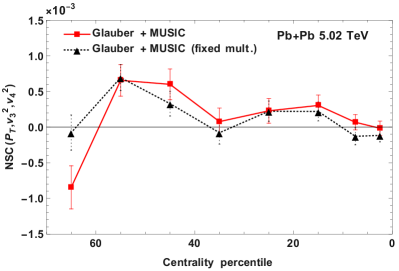
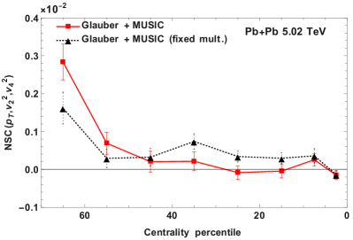
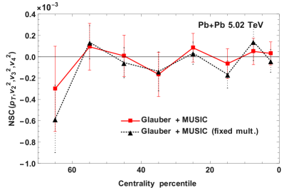
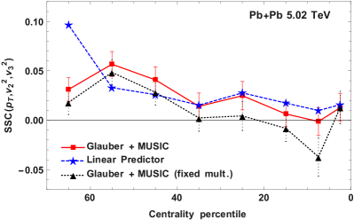
In Figs. 5, 7, and 6 are shown the third order cumulants for $p_{T}$ and two different coefficients of the harmonic flow. For all the third order correlations considered, the magnitude of the scaled cumulant is small, as it measures only genuine third order correlations. The linear predictor (15), based on initial correlations only, describes the full hydrodynamic calculation for centralities 0-60%. The cumulants involving $v_{4}$ cannot be predicted using a linear predictor, but could serve a precise measure of nonlinearities between harmonic flows of different order. The fourth order normalized symmetric cumulant $NSC(p_{T},v_{2}^{2},v_{3}^{2},v_{4}^{2})$ is compatible with zero within the statistical accuracy of our calculation (Fig. 8).

V Symmetric cumulants for collisions of deformed nuclei

In central collisions of deformed nuclei the relative orientation of the axes of deformation of the two nuclei determines the initial ellipticity, entropy, and the size of the fireball Heinz:2004ir ; Goldschmidt:2015kpa ; Rybczynski:2012av ; Haque:2011aa ; Chatterjee:2014sea ; Adamczyk:2015obl ; Giacalone:2020awm . As a consequence, the final elliptic flow, the average transverse momentum and/or the multiplicity may be correlated with the initial orientation of the deformation axes in a collision. In central collisions of deformed nuclei, tip-on-tip collision lead to a large transverse momentum and small elliptic flow, while body-on-body collisions lead to a smaller transverse momentum but larger elliptic flow Giacalone:2019pca . This effect reduces the value of the correlation coefficient $\rho(p_{T},v_{2}^{2})$ in central U+U collisions.

Figure 9: The correlation coefficient between the average transverse momentum and the elliptic flow coefficient $\rho(p_{T},v_{2}^{2})$ for central U+U collisions at $\sqrt{s_{NN}}=193$ GeV as a function of centrality. Results for collisions of deformed nuclei with and without fluctuations in entropy deposition are denoted with red squares and black triangles respectively. The results for spherical nuclei are represented using blue dots.

Figure 10: Same as in Fig. 9 but for the triangular flow.

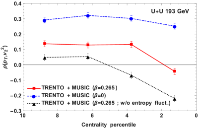
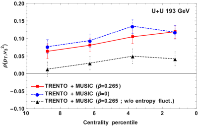
In this section symmetric cumulants for U+U collisions at $\sqrt{s_{NN}}=193$ GeV are studied. Initial conditions from the TRENTO model (with parameter $p=0$) Moreland:2014oya are evolved using the 2-dimensional version of the MUSIC hydrodynamic code. We compare three scenarios for the initial conditions : collisions of uranium nuclei with deformation parameter $\beta=0.265$ and fluctuations of entropy deposition from each participant (exponential distribution), collisions of spherical uranium nuclei ($\beta=0$), and collisions of deformed uranium nuclei ($\beta=0.265$) without fluctuations of entropy deposition. In Figs. 9 and 10 are shown the correlation coefficients of the average transverse momentum and harmonic flow. The value of the correlation coefficient $\rho(p_{T},v_{2}^{2})$ is smaller for collisions of deformed nuclei than in the case of spherical nuclei, as expected. We note, that the correlation coefficient for initial conditions without fluctuations in entropy deposition is smaller than in the cases with fluctuations for both correlation coefficients $\rho(p_{T},v_{2}^{2})$ and $\rho(p_{T},v_{3}^{2})$. In central collisions the covariances of the harmonic flow observables with multiplicity are small. We have checked that for the centrality bins used in our study for U+U collisions , the corrections for multiplicity fluctuations to the correlation coefficients and higher order symmetric cumulants are small. In the following we show only the uncorrected symmetric cumulants for U+U collisions.

Figure 11: The normalized symmetric cumulant of the average transverse momentum, the elliptic, and the triangular flow coefficients $NSC(p_{T},v_{2}^{2},v_{3}^{2})$ for central U+U collisions at $\sqrt{s_{NN}}=193$ GeV as function of centrality. Results for collisions of deformed nuclei with and without fluctuations in entropy deposition are denoted with red squares and black triangles respectively. The results for spherical nuclei are represented using blue dots.

Figure 12: Same as in Fig. 11 but for the normalized symmetric cumulant of the average transverse momentum, the triangular and quadratic flow coefficients $NSC(p_{T},v_{3}^{2},v_{4}^{2})$.

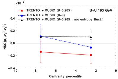
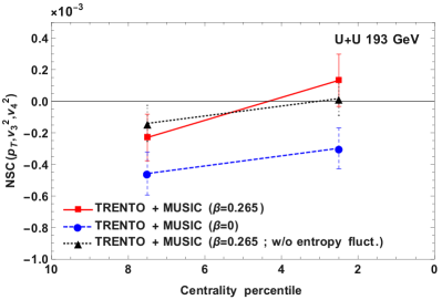
The third order symmetric cumulants $NSC(p_{T},v_{2}^{2},v_{3}^{2})$ is smaller for collisions of deformed nuclei with fluctuations of entropy deposition than in the other two scenarios studied (Fig. 11). On the other hand, the normalized symmetric cumulant $NSC(p_{T},v_{3}^{2},v_{4}^{2})$ is smaller for collisions of spherical nuclei than in calculations using deformed uranium nuclei (Fig. 12).

Figure 13: Same as in Fig. 11 but for the normalized symmetric cumulant of the average transverse momentum, the multiplicity and the elliptic flow coefficient $NSC(p_{T},N,v_{2}^{2})$. Symbols as in Fig. 11.

Figure 14: The fourth order symmetric cumulant of the average transverse momentum, the multiplicity, the elliptic, and the triangular flow coefficients $NSC(p_{T},N,v_{2}^{2},v_{3}^{2})$. Symbols as in Fig. 11.

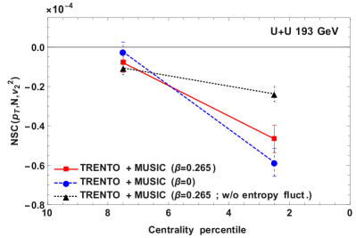
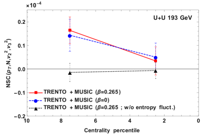
The collective flow in central collisions of deformed nuclei is dominated by the fluctuations in the initial entropy and its azimuthal asymmetries. Therefore, it is interesting to study symmetric cumulants involving not only the average transverse momentum and harmonic flow, but also the multiplicity in the event. Please note, that the results for the symmetric cumulants involving multiplicity as one of the observables may depend on the definition of the centrality bin. In order to reduce the bias from centrality cuts, that observables could be calculated experimentally using centrality bins based on forward rapidity observables, i.e. the forward transverse energy. The symmetric cumulant $NSC(p_{T},N,v_{2}^{2})$ is sensitive to the fluctuations of entropy deposition from the participant nucleons (Fig. 13). Fluctuations in entropy deposition increase the magnitude of $NSC(p_{T},N,v_{2}^{2})$. The fourth order cumulant $NSC(p_{T},N,v_{2}^{2},v_{3}^{2})$ is positive for simulations involving fluctuations in the entropy deposition in the initial states (Fig. 14), while it is compatible with zero for simulations without entropy fluctuations in the initial state. The normalized symmetric cumulant $NSC(p_{T},v_{2}^{2},v_{3}^{2},v_{4}^{2})$ (not shown) is compatible with zero within our statistics.

VI Scaled symmetric cumulants

Figure 15: The scaled symmetric cumulant of the average transverse momentum and the squares of the elliptic and triangular flow coefficients $SSC(p_{T},v_{2}^{2},v_{3}^{2})$ in Pb+Pb collisions as a function of centrality (red squares). The blue stars denote the results obtained from the linear predictor 15 and the black triangles show the scaled symmetric cumulant for observables corrected for multiplicity fluctuations 14.

The normalized symmetric cumulants (22) and (23) involve, in the denominator, averages of the observables for which the cumulant is calculated. However, the interpretation of the results is less obvious than for the correlation coefficient. Moreover, the average transverse momentum in a collision depends on many effects Bozek:2012fw , the freeze-out procedure, the bulk viscosity, the prequilibrium flow, or simply the experimental transverse momentum range. The linear predictor for the average transverse momentum in an event (15) can predict only deviations from the mean.

An alternative normalization of the symmetric cumulants would involve the standard deviations of the observables in the denominator and we get the scaled symmetric cumulants,

$$SSC(A,B,C)=\frac{SC(A,B,C)}{\sqrt{Var(A)Var(B)Var(C)}}$$ (24)

and

$$SSC(A,B,C,D)=$$

$$\frac{SC(A,B,C,D)}{\sqrt{Var(A)Var(B)Var(C)Var(D)}}$$ (25)

The scaled symmetric cumulant has the advantage that its prediction from the initial state does not require additional input on the value of the average transverse momentum (from simulation or experiment). The value of the scaled symmetric cumulants can be fully predicted using the linear hydrodynamic response.

Figure 16: The scaled symmetric cumulant of the average transverse momentum, the elliptic, and the triangular flow coefficients $SSC(p_{T},v_{2}^{2},v_{3}^{2})$ for central U+U collisions at $\sqrt{s_{NN}}=193$ GeV as a function of centrality. Results for collisions of deformed nuclei with and without fluctuations in entropy deposition are denoted with red squares and black triangles respectively. The results for spherical nuclei are represented using blue dots.

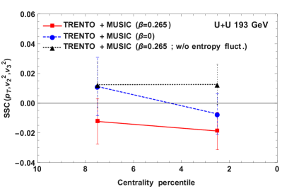
The scaled symmetric cumulants show a very similar behavior as the normalized symmetric cumulants discussed in previous sections. This can be seen in the examples chosen for Pb+Pb collisions (Fig. 15) and U+U collisions (Fig. 16). The numerical values are larger for the scaled symmetric cumulants than for the normalized symmetric cumulants. Alone the change from the normalization by the average transverse momentum to the normalization by its standard deviation yields a factor in the range: $20-100$.

VII Summary

Flow observables are fluctuating from event to event. Moments from the values of several flow observables in the event can be constructed. We propose to measure higher order symmetric cumulants between the average transverse momentum and harmonic flow coefficients. Symmetric cumulants of order $n$ measure genuine $n$ order correlations between the observables studied.

Symmetric cumulants can be normalized by the averages or by the standard deviations of the considered observables. Such normalized cumulants involving the elliptic flow, the triangular flow, and the transverse momentum could be predicted from the initial conditions. Their study could serve as a sensitive probe of higher order correlations in the initial state of the evolution in the collision. Further cumulants involving flow harmonics of higher order could serve as a probe of nonlinearities in the hydrodynamic response.

We present predictions based on the hydrodynamic model for collisions of spherical (Pb+Pb) or deformed (U+U) nuclei. The symmetric cumulants involving the elliptic and triangular flows obtained from the full hydrodynamic calculation can be well described using a linear predictor from the initial state. Our predictions could be compared to future experimental measurements.

References

- (1) J.-Y. Ollitrault, J. Phys. Conf. Ser. 312, 012002 (2011)
- (2) U. Heinz and R. Snellings, Ann.Rev.Nucl.Part.Sci. 63, 123 (2013)
- (3) C. Gale, S. Jeon, and B. Schenke, Int.J.Mod.Phys. A28, 1340011 (2013)
- (4) W. Broniowski, M. Chojnacki, and L. Obara, Phys. Rev. C80, 051902 (2009)
- (5) P. Bożek, Phys. Rev. C93, 044908 (2016)
- (6) P. Bożek and H. Mehrabpour, Phys. Rev. C 101, 064902 (2020)
- (7) B. Schenke, C. Shen, and D. Teaney, Phys. Rev. C 102, 034905 (2020)
- (8) G. Giacalone, F. G. Gardim, J. Noronha-Hostler, and J.-Y. Ollitrault(4 2020), arXiv:2004.01765 [nucl-th]
- (9) G. Aad et al. (ATLAS), Eur. Phys. J. C79, 985 (2019)
- (10) G. Giacalone, Phys. Rev. Lett. 124, 202301 (2020)
- (11) G. Giacalone, Phys. Rev. C 102, 024901 (2020)
- (12) G. Aad et al. (ATLAS), ATLAS-CONF-2021-001(2021)
- (13) J. Jia (STAR), talk presented at 6th International Conference on the Initial Stages in High-Energy Nuclear Collisions. Revhovot, 10-15 January (2021)
- (14) G. Giacalone, B. Schenke, and C. Shen, Phys. Rev. Lett. 125, 192301 (2020)
- (15) A. Bilandzic, C. H. Christensen, K. Gulbrandsen, A. Hansen, and Y. Zhou, Phys. Rev. C 89, 064904 (2014)
- (16) C. Mordasini, A. Bilandzic, D. Karakoç, and S. F. Taghavi, Phys. Rev. C 102, 024907 (2020)
- (17) Z. Moravcova, K. Gulbrandsen, and Y. Zhou(5 2020), arXiv:2005.07974 [nucl-th]
- (18) B. Schenke, S. Jeon, and C. Gale, Phys. Rev. C 82, 014903 (2010)
- (19) B. Schenke, S. Jeon, and C. Gale, Phys. Rev. Lett. 106, 042301 (2011)
- (20) J.-F. Paquet, C. Shen, G. S. Denicol, M. Luzum, B. Schenke, S. Jeon, and C. Gale, Phys. Rev. C 93, 044906 (2016)
- (21) P. Bożek, W. Broniowski, M. Rybczynski, and G. Stefanek, Comput. Phys. Commun. 245, 106850 (2019)
- (22) A. Olszewski and W. Broniowski, Phys. Rev. C96, 054903 (2017)
- (23) F. G. Gardim, F. Grassi, M. Luzum, and J.-Y. Ollitrault, Phys. Rev. C85, 024908 (2012)
- (24) Z. Qiu and U. W. Heinz, Phys. Rev. C84, 024911 (2011)
- (25) H. Niemi, G. S. Denicol, H. Holopainen, and P. Huovinen, Phys. Rev. C87, 054901 (2013)
- (26) A. Mazeliauskas and D. Teaney, Phys. Rev. C93, 024913 (2016)
- (27) P. Bożek and W. Broniowski, Phys. Rev. C96, 014904 (2017)
- (28) C. Zhang, A. Behera, S. Bhatta, and J. Jia(2021), arXiv:2102.05200 [nucl-th]
- (29) U. W. Heinz and A. Kuhlman, Phys. Rev. Lett. 94, 132301 (2005)
- (30) A. Goldschmidt, Z. Qiu, C. Shen, and U. Heinz, Phys. Rev. C 92, 044903 (2015)
- (31) M. Rybczynski, W. Broniowski, and G. Stefanek, Phys. Rev. C 87, 044908 (2013)
- (32) M. R. Haque, Z.-W. Lin, and B. Mohanty, Phys. Rev. C 85, 034905 (2012)
- (33) S. Chatterjee and P. Tribedy, Phys. Rev. C 92, 011902 (2015)
- (34) L. Adamczyk et al. (STAR), Phys. Rev. Lett. 115, 222301 (2015)
- (35) J. S. Moreland, J. E. Bernhard, and S. A. Bass, Phys. Rev. C 92, 011901 (2015)
- (36) P. Bożek and W. Broniowski, Phys. Rev. C85, 044910 (2012)