Bayesian Deep Basis Fitting for Depth Completion with Uncertainty

Abstract

In this work we investigate the problem of uncertainty estimation for image-guided depth completion. We extend Deep Basis Fitting (DBF) [57] for depth completion within a Bayesian evidence framework to provide calibrated per-pixel variance. The DBF approach frames the depth completion problem in terms of a network that produces a set of low-dimensional depth bases and a differentiable least squares fitting module that computes the basis weights using the sparse depths. By adopting a Bayesian treatment, our Bayesian Deep Basis Fitting (BDBF) approach is able to 1) predict high-quality uncertainty estimates and 2) enable depth completion with few or no sparse measurements. We conduct controlled experiments to compare BDBF against commonly used techniques for uncertainty estimation under various scenarios. Results show that our method produces better uncertainty estimates with accurate depth prediction.

1 Introduction

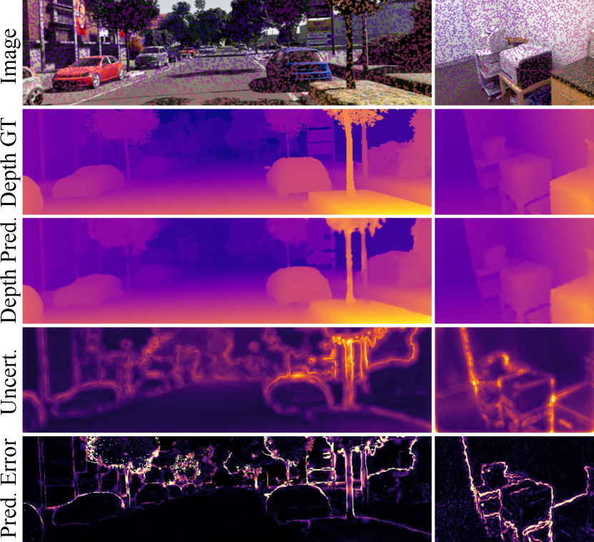
Figure 1: Qualitative results of our method, Bayesian Deep Basis Fitting (BDBF), which outputs uncertainty estimates with depth completion.

As we seek to incorporate learned modules in safety critical applications such as autonomous driving, reliable uncertainty estimation becomes as critical as prediction accuracy  [63]. Depth completion is one such task where well-calibrated uncertainty estimates can help to enable robust machine perception. Deep Convolutional Neural Networks (CNNs) are commonly used to solve structured regression problems like depth prediction due to their strong expressive power and inductive bias [14]. However, in its native form, a CNN only produces a point estimate, which offers few insights into whether or where its output should be trusted. Many probabilistic deep learning methods have been proposed to address this issue [47, 19], but they often fail to output calibrated uncertainty [25] or become susceptible to distributional shift [53]. Moreover, these methods can be expensive to compute due to the need for test time sampling [20] or inference over multiple models [39].

In this work, we propose a method for depth completion with uncertainty estimation that avoids the above limitations. Our approach builds on the idea of Deep Basis Fitting (DBF) [57]. DBF replaces the last layer of a depth completion network with a set of data-dependent weights. These weights are computed by a differentiable least squares fitting module between the penultimate features and the sparse depths. The network can also be seen as an adaptive basis function which explicitly models scene structure on a low-dimensional manifold [5, 64]. It can be used as a replacement to the final layer (with no change to the rest of the network or training scheme), which greatly improves depth completion performance.

We extend DBF by formulating it within a Bayesian evidence framework [4]. This is done by placing a prior distribution on the DBF weights and marginalizing it out during inference. Such last-layer probabilistic approach have been shown to be reasonable approximations to full Bayesian Neural Networks [37], while providing the advantage of tractable inference [51]. This is conceptually similar to Neural Linear Models (NLMs) [62] with the notable distinction that we perform Bayesian linear regression on each image as opposed to the entire dataset.

A Bayesian treatment also enables depth completion with highly sparse data. In DBF, when the number of sparse depths falls below the dimension of the bases, the underlying linear system becomes under-determined. We show that by learning a shared prior across images, our method is able to handle any number of sparse depth measurements.

We name our approach Bayesian Deep Basis Fitting (BDBF) and summarize its advantages: 1) It can be used as a drop-in replacement to the final layer of many depth completion networks and outputs uncertainty estimates (in the form of per-pixel variance). 2) Compared to other uncertainty estimation techniques, it produces higher quality uncertainty with one training session, one saved model and one forward pass, without needing extra parameters or modifications to the loss function. 3) It can handle any sparsity level, with performance degrading gracefully towards a pure monocular method when the number of depth measurements goes to zero.

2 Related Work

2.1 Uncertainty Estimation for Neural Networks

We start by reviewing uncertainty estimation techniques for neural networks. There are two types of uncertainty that one could model: epistemic (model), which describe the uncertainty in the model and aleatoric (data), which reflects the inherent noise in the data [36]. Modeling uncertainty in neural networks can be achieved by placing probabilistic distributions on network weights. Such networks are called Bayesian Neural Networks (BNN) [47]. Direct inference in BNNs is intractable for continuous variables, and different approximation techniques have been explored [47, 32, 24, 6, 49, 48, 33]. However, they don’t scale well to large datasets and complex models, and are thus impractical for current vision tasks.

Gal et al. [20] proposed the use of dropout as an approximate variational inference method for BNNs. However, their method requires multiple forward passes to obtain Monte Carlo model estimates at test time. Another research direction is assumed density filtering (ADF) [52] which can be viewed as a single Expectation Propagation pass. Gast et al. [22] chose to propagate activation uncertainties without probabilistic weights in a lightweight manner, which requires modifying the layer operations based on moment matching.

Predictive methods directly output mean and variance of some parametric distribution by minimizing the negative-log likelihood (NLL) loss [50]. They only require small changes to the original network by adding a variance prediction head. This simplicity makes it a popular choice among recent works [34, 42].

Ensemble methods either train multiple models independently with different initializations (bootstrap) [39] or save several copies of weights at different stages during training (snapshot) [29]. These methods only model epistemic uncertainty but can be combined with a predictive one to model data uncertainty. They achieve good performances in various experimental settings [26, 55, 31], but still need multiple inference passes at test time, which makes them less suitable for resource constrained platforms.

Table 1 summarizes the aforementioned approaches and highlights the difference compared to ours. In Sec. 4.1 we describe in detail the methods that we evaluate against.

Method	#T	#M	#F	Alea.	Epis.
Predictive [50, 34]	1	1	1	✓
Dropout (Predictive) [20, 34]	1	1	K	(✓)	✓
Snapshot (Predictive) [29]	1	K	K	(✓)	✓
Bootstrap (Predictive) [39]	K	K	K	(✓)	✓
Proposed (BDBF)	1	1	1	✓	✓

Table 1: Comparison of different uncertainty estimation techniques. The first three columns represent number of training sessions (T), copies of model saved (M), and number of forward passes (F) at test time respectively. Last two columns indicate whether a method estimates data or model uncertainties. Dropout, snapshot and bootstrap ensemble can all be combined with a predictive approach to model data uncertainty. BDBF has the same complexity as predictive methods.

2.2 Uncertainty Estimation in Depth Completion

Great progress has been made in the past few years on depth completion ranging from high-density completion for RGB-D/ToF cameras [41, 17, 72, 74], to mid-density completion from LiDAR sensors [68, 46, 11, 65, 10, 9, 75, 40, 71, 73]. Recently, there has also been rising interests in low-density completion from map points generated by Visual-SLAM or Visual-Inertial Odometry [69, 70, 59, 76]. Unlike systems that are designed for a particular sparsity or sensing modality, our proposed method can be seen as a general component for depth completion similar to DBF [57].

A complete review of depth completion literature is out of the scope of this work, we instead focus on methods that also estimate uncertainty. Gansbeke et al. [21] predict depth and confidence weights for both color and depth branch and fuse them based on the confidence maps. Qiu et al. [56] adopt a similar strategy, but additionally guide the depth branch via surface normal prediction. Xu et al. [71] use a shared encoder and multiple decoders to predict surface normal, coarse depth and confidence, then use an anisotropic diffusion process to produce refined depth. Park et al. [54] instead use a single encoder-decoder network to predict initial depth, affinities and confidence before applying a non-local spatial propagation to produce the final depth. Note that the uncertainties produced by the above methods are not calibrated and are only used internally. Therefore, they are not readily useful to downstream tasks that require probabilistic reasoning. This type of uncertainty estimation can also be seen as a simplified version of the predictive method in [50] without the NLL loss.

Few works have tried to evaluate the quality of depth completion uncertainty. Eldesokey et al. [15] present a probabilistic normalized convolution [16] that estimates confidence of both input sparse depths and output dense prediction, for unguided depth completion. Gustafsson et al. [26] compared several uncertainty estimation methods applied to depth completion in the same spirit as [55]. We follow their approach and provide a systematic comparison of our proposed method against the best performing schemes from [26, 55] and demonstrate superior performance and efficiency across a range of datasets.

3 Method

3.1 Problem Formulation

Let $\mathcal{D}=\{(\mathbf{x}_{n},\mathbf{y}_{n})\}_{n=1}^{N_{\mathcal{D}}}$ be a dataset containing $N_{\mathcal{D}}$ samples. We wish to learn a neural network $f$ that maps $\mathbf{x}$ to $\mathbf{y}$. In depth completion, the input $\mathbf{x}$ is usually an image and sparse depth pair $(I,S)$, and the output $\mathbf{y}$ is the predicted depth map $D$. We refer to $f_{\theta}$ as the basis network and its output $\Phi$ a set of depth bases [57]. $\Phi$ is then reduced by a linear layer $f_{\mathbf{w}}$ to $\mathbf{z}$, which is then mapped to positive depth values via a nonlinear activation function $g$.

$$\mathbf{y}=f(\mathbf{x})=g\circ f_{\mathbf{w}}\circ f_{\theta}(\mathbf{x})=g\circ f_{\mathbf{w}}(\Phi)=g(\mathbf{z})$$ (1)

With a slight abuse of notation, we call $\mathbf{z}$ the latent variable and choose $g$ to be the exponential function [14], so $\mathbf{z}$ effectively corresponds to log depth. An overview of our method is shown in Figure 2.

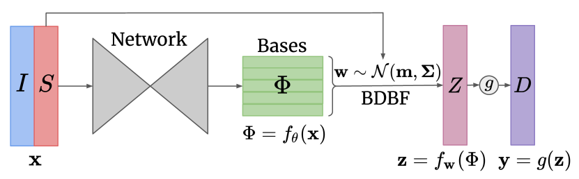
Figure 2: An overview of BDBF for depth completion. The input to the network is an RGB image $I$ and optionally a sparse depth map $S$. The network produces a $M$-dimensional depth bases $\bm{\Phi}$, which has the same spatial resolution as $I$. BDBF then solves for the weights $\mathbf{w}$ given the sparse depth at valid pixel locations. $\mathbf{w}$ can then be used to reduce the bases into a single channel latent prediction $Z$, before going through the activation $g$ to produce depth $D$.

3.2 Bayesian Deep Basis Fitting

We choose to model the distribution of each pixel in the latent space $\mathbf{z}$ rather than in the target space $\mathbf{y}$, since depth is strictly positive and may span several orders of magnitude [61]. Assuming Gaussian noise in the latent space, we define our model to be

$$z_{i}=\mathbf{w}^{\top}\bm{\phi}_{i}+\epsilon_{i},\quad\epsilon_{i}\sim\mathcal{N}(0,\beta^{-1})$$ (2)

where $\bm{\phi}_{i}$ denotes the basis entries corresponding to the latent pixel value $z_{i}$ and $\beta\in\mathbb{R}$ is a precision parameter that corresponds to the inverse variance of the noise. Assuming that the errors at each pixel are independent, the likelihood function is

$$p(\mathbf{z}|\mathbf{x},\mathbf{w}) =\mathcal{N}(\mathbf{z}|\bm{\Phi}\mathbf{w},\beta^{-1}\mathbf{I})$$ (3)

here $\bm{\Phi}$ is the $N\times M$ design matrix with $N$ the number of sparse depths and $M$ the dimension of $\mathbf{w}$. It is assembled by extracting the basis entries at the pixel locations specified by $S$.

Given a suitable prior on the last-layer weights $p(\mathbf{w})=\mathcal{N}(\mathbf{m}_{0},\alpha^{-1}\bm{\Sigma}_{0})$, where $\alpha\in\mathbb{R}$ is a precision parameter to scale the covariance $\bm{\Sigma}_{0}$, the posterior distribution of $\mathbf{w}$ can be computed analytically following Bayes’ rule [4]:

$$p(\mathbf{w}|\mathbf{x},\mathbf{z}) =\mathcal{N}(\mathbf{m},\bm{\Sigma})$$ (4)

$$\propto\mathcal{N}(\mathbf{w}|\mathbf{m}_{0},\alpha^{-1}\bm{\Sigma}_{0})\cdot\mathcal{N}(\mathbf{z}|\bm{\Phi}\mathbf{w},\beta^{-1}\mathbf{I})$$ (5)

where the mean and covariance are given by

$$\mathbf{m} =\bm{\Sigma}(\alpha\bm{\Sigma}_{0}^{-1}\mathbf{m}_{0}+\beta\bm{\Phi}^{\top}\mathbf{z})$$ (6)

$$\bm{\Sigma} =(\alpha\bm{\Sigma}_{0}^{-1}+\beta\bm{\Phi}^{\top}\bm{\Phi})^{-1}$$ (7)

The latent predictive distribution for a pixel at test time is

$$p(z_{*}|\mathbf{x},\mathbf{z}) =\int p(z_{*}|\mathbf{w})p(\mathbf{w}|\mathbf{x},\mathbf{z})d{\mathbf{w}}$$ (8)

$$=\mathcal{N}(z_{*}|\mathbf{m}^{\top}\bm{\phi}_{*},\bm{\phi}_{*}^{\top}\bm{\Sigma}\bm{\phi}_{*})$$ (9)

The Gaussian assumption is made solely for the purpose of tractable inference. In practice, the shape of the predictive distribution depends heavily on the loss function. Since we use L1 loss for training, we employ a Laplace distribution as its parametric form for evaluating uncertainty [31, 5]. Additionally, a robust norm like Huber [30] can be applied if outliers are present in the target [67] .

3.3 Training

Loss Function. The standard way of learning such models is by maximizing the marginal likelihood function with respect to the parameters $\theta$ of the basis function $f_{\theta}$,

$$\begin{split}\log p(\mathbf{z}|\mathbf{x},\alpha,\beta)&=\frac{1}{2}(N\ln\beta+M\ln\alpha-N\ln 2\pi\\ &\qquad-E(\mathbf{m})+\ln|\bm{\Sigma}|-\ln|\bm{\Sigma}_{0}|)\end{split}$$ (10)

$$E(\mathbf{w}) =\beta\|\mathbf{z}-\bm{\Phi}\mathbf{w}\|^{2}+\alpha\|\mathbf{w}-\mathbf{m}_{0}\|^{2}_{\bm{\Sigma}_{0}}$$ (11)

where $\|\mathbf{v}\|_{\mathbf{A}}=\mathbf{v}^{\top}\mathbf{A}^{-1}\mathbf{v}$ is the Mahalanobis norm. This is known in literature as type 2 maximum likelihood [4].

Directly maximizing (10) has two practical issues. First, one needs to estimate the hyperparameters $\alpha$ and $\beta$, which adds large overhead during training. Second, gradients need to be back-propagated through costly operations like matrix inversion and determinant. Together, they pose challenges to the training phase and often produce empirically similar results to a point estimate [62]. We avoid these issues by assuming sufficient sparse points in training ($N\gg M$). This renders the linear system over-determined, which allows us to treat the prior $p(\mathbf{w})$ as infinitely broad. The solution in (6) therefore reduces to a maximum likelihood (ML) one which can be computed efficiently in one pass [4].

$$\mathbf{w}_{\mathrm{ML}} =(\bm{\Phi}^{\top}\bm{\Phi})^{-1}\bm{\Phi}^{\top}\mathbf{z}$$ (12)

$$\beta_{\mathrm{ML}}^{-1} =\frac{1}{N}\|\mathbf{z}-\bm{\Phi}\mathbf{w}_{\mathrm{ML}}\|^{2}$$ (13)

The predicted mean and variance of $z_{*}$ at training time are given by the following according to (9)

$$\mu=\mathbf{w}_{\mathrm{ML}}^{\top}\bm{\phi},\quad\sigma^{2}=\beta_{\mathrm{ML}}^{-1}\bm{\phi}^{\top}(\bm{\Phi}^{\top}\bm{\Phi})^{-1}\bm{\phi}$$ (14)

Given the above results, we can minimize the Negative Log-Likelihood Loss (NLL) assuming a Laplace distribution [31], which is defined for a single pixel as

$$-\log p(z|\mu,b)\propto\frac{|\mu-z|}{b}+\log{b},\quad 2b^{2}=\sigma^{2}$$ (15)

However, this would still involve back-propagation through a costly matrix inversion as in (12). We find in our experiments that this sometimes causes numerical instability during training and incurs a visible decrease in prediction accuracy. Therefore, we opt to minimize directly the L1 loss for supervised learning. This allows our network to be trained in its original form without suffering from the performance drop caused by the NLL loss [43].

Uncertainty Calibration. Not using the likelihood loss comes with the risk of over-confidence in uncertainty estimation, since there is no explicit penalty on the variance prediction. As the number of parameters in $\theta$ is usually on the order of millions, the noise variance $\beta^{-1}$ will be pushed towards zero [51]. One solution is to regularize $\theta$ using an L2 regularization term in the optimizer. This introduces an extra hyperparameter to tune: a small regularization would not prevent overfitting, while a large one will render the feature bases inexpressive [66]. We notice empirically that the amount of overconfidence in our method is consistent during training and validation. Therefore, we take a pragmatic approach and propose to solve this problem in terms of estimator consistency [2], measured by normalized estimation error squared (NEES). For a Laplace distribution, NEES is defined as $\varepsilon=(\mu-z)^{2}/b^{2}$. We record the average NEES $\bar{\varepsilon}$ at training time for the last epoch, and use it to scale the variance accordingly during inference with $\bar{\sigma}^{2}=\bar{\varepsilon}\sigma^{2}$, which attempts to make the final prediction consistent. Note that the scaling factor is computed entirely at training without any additional data and NEES is not used as a loss function.

Shared Prior. Although the prior $p(\mathbf{w})$ is not used in training, we still need it for inference. Rather than estimating a different prior for each image, we make another simplifying assumption that there exists a shared prior for the entire dataset. This aligns with our observation from experiments that $p(\mathbf{w})$ shows a relatively sharp peak. Given our training strategy, we adopt a frequentist approach and collect all ML solutions of weights $\mathbf{w}_{\mathrm{ML}}$ within one training epoch. The mean, $\mathbf{m}_{0}$, and covariance, $\bm{\Sigma}_{0}$, can then be computed from this set. Having a shared prior enables robust depth completion from a few sparse depth measurements.

3.4 Inference

Inference follows the standard evidence framework [4]. We use EM [13] to estimate the hyperparameters $\alpha$ and $\beta$. The re-estimation equations are obtained by maximizing the expected complete-data log likelihood with respect to $\alpha$, $\beta$

$$\alpha^{-1} =\frac{1}{M}\left(\|\mathbf{m}-\mathbf{m}_{0}\|^{2}_{\bm{\Sigma_{0}}}+\operatorname{tr}(\bm{\Sigma}_{0}^{-1}\bm{\Sigma})\right)$$ (16)

$$\beta^{-1} =\frac{1}{N}\left(\|\mathbf{z}-\bm{\Phi}\mathbf{m}\|^{2}+\operatorname{tr}(\bm{\Phi}^{\top}\bm{\Phi}\bm{\Sigma})\right)$$ (17)

where $\operatorname{tr}(\cdot)$ is the matrix trace operator. The re-estimated $\alpha$ and $\beta$ are then plugged back into (6) and (7) to recompute $\mathbf{m}$ and $\bm{\Sigma}$. We initialize this process empirically with $\alpha=1$ and $\beta=\sqrt{N}$ and set the maximum number of iterations to 8. In practice we reach convergence within 2 to 3 iterations when $N\gg M$, thus incurring only a small computation overhead. In the extreme case when $N\rightarrow 0$, we rely on the shared prior alone for a pure monocular prediction.

$$\mu=\mathbf{m}_{0}^{\top}\bm{\phi},\quad\sigma^{2}=\bm{\phi}^{\top}\bm{\Sigma}_{0}\bm{\phi}$$ (18)

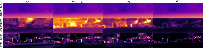
Figure 3: Qualitative results of all methods trained and test with 5% sparsity on VKITTI2.

4 Evaluation

In this section, we thoroughly evaluate our proposed method (bdbf). We show with extensive experimental results on three different datasets and various sparsity settings that our method outperforms baseline approaches in uncertainty estimates with accurate depth prediction, and remains resilient to sparsity change and domain shift.

4.1 Baselines

We describe three baselines for uncertainty estimation that we compare to, which are shown to have strong performance [55, 26] and can be evaluated under controlled settings. As discussed in Section 3.2, all methods output mean and variance of the latent prediction before $g(\cdot)$, and are trained with either L1 loss or its NLL variant (15).

For empirical methods, we choose Snapshot Ensemble [29] (snap) which can be completed in one training session such that all methods have the same training budget. The mean and variance are computed using $K$ snapshots.

$$\mu=\frac{1}{K}\sum_{i=1}^{K}\mu_{i},\quad\sigma^{2}=\frac{1}{K}\sum_{i=1}^{K}(\mu_{i}-\mu)^{2}$$ (19)

For predictive methods (log) [50], we attach a variance prediction head parallel to the depth prediction and train with the NLL loss. Finally, we combine the above two (snap+log) [34] to form a predictive ensemble method.

$$\mu=\frac{1}{K}\sum_{i=1}^{K}\mu_{i},\quad\sigma^{2}=\frac{1}{K}\sum_{i=1}^{K}\left((\mu_{i}-\mu)^{2}+\sigma_{i}^{2}\right)$$ (20)

4.2 Datasets

Virtual KITTI 2. The VKITTI2 dataset [7] is an updated version to its predecessor [18]. We use sequences 2, 6, 18 and 20 with variations clone, morning, overcast and sunset for training and validation, and clone in sequence 1 for testing. This results in 6717 training and 447 testing images. The sparse depths are generated by randomly sampling pixels that have a depth less than 80m [26]. Ground truth depths are also capped to 80m following common evaluation protocols. All images are downsampled by half.

NYU Depth V2. The NYU-V2 [60] dataset is comprised of various indoor scenes recorded by an off-the-shelf RGB-D camera. We use the 1449 densely labeled pairs of aligned RGB and depth images. and split it into approximately 75% training and 25% testing. The same depth sampling strategy is adopted as above. Note that we intentionally choose this small dataset (as opposed to the full) to evaluate uncertainty estimation under data scarcity [66].

KITTI Depth Completion. We also evaluate on the KITTI depth completion dataset [68] following its official train/val split. For all experiments other than the official submission, we down sample both the image and depth by half.

4.3 Implementation Details

Network architecture. We use the same basis network for all methods, which is an encoder-decoder architecture with skip connection similar to that in [57]. We use a MobileNet-V2 [61] pretrained on ImageNet [38]. The decoder outputs a set of multi-scale bases [57], which are then upsampled to the input resolution and concatenated together to form a final 63-dimensional basis. For baseline methods we initialize the bias of depth prediction head with the average log depth of the dataset and let the variance head predict an initial variance of 1. Our method, however, requires no initialization. When using sparse depths as network input, we adopt the two-stage approach from [70] which first scaffolds the sparse depths by interpolation and then fuses it with the first layer of the encoder via convolution. Note that this depth pre-processing step is orthogonal to the uncertainty estimation techniques and we choose this approach for its simplicity and applicability to both mid- and low-sparsity. All networks use the same setup unless otherwise stated.

Training parameters. For training we use the Adam optimizer [35] with an initial learning rate of 2e-4 and reduce it by half every 5 epochs following [45, 57]. We train our method for 20 epochs and all others for 30. This is to account for the increased training time using our method. For Snapshot Ensemble,we follow the original paper [29] and use the cyclic annealing scheduler from [44] with the same initial learning rate as before. we train for 5 epochs per cycle, and discard the worst snapshot, which leaves us with 5 snapshots. All training is carried out on a single Tesla V100 GPU with the same batch size and random seed. For data augmentation we apply a random horizontal flip with a probability of 0.5 and a small color jitter of 0.02.

4.4 Metrics

Depth prediction metrics. We evaluate depth completion performance using standard metrics [14]. Specifically, we report MAE, RMSE and accuracy ($\delta$-threshold) on depth. Due to space limitation, we only report $\delta_{1}<1.25$.

Uncertainty estimation metrics. Unlike depth prediction which can be compared to ground truth, the true probability density function of depth is not available. This makes evaluating uncertainty estimates a difficult task in itself. We describe three popular metrics from the literature for evaluating uncertainty estimates. Note that each metric has its own advantages and drawbacks, we seek to provide a more comprehensive evaluation by reporting all three.

1) Area Under the Sparsification Error curve (AUSE)$\downarrow$. Sparsification plots [1] are commonly used for measuring the quality of uncertainty estimates. Given an error metric (e.g. MAE), we sort the prediction errors by their uncertainty in descending order and compute the error metric repeatedly by removing a fraction (e.g. 1%) of the most uncertain subset. An oracle sparsification curve is obtained by sorting using the true prediction errors. AUSE is the area between the sparsification curve and the oracle curve. This normalizes the oracle out and can be used to compare different methods [31]. Note that AUSE is a relative measure of uncertainty quality, since its computation relies on the order of predicted uncertainties.

2) Area Under the Calibration Error curve (AUCE)$\downarrow$. For an absolute measure of uncertainty estimation quality, [26] proposes to generalize the Expected Calibration Error (ECE) [25] metric to regression. For Laplace distributions, given mean $\mu$ and variance $\sigma^{2}$, we construct prediction intervals $\mu\pm\Psi^{-1}(\frac{p+1}{2})b$ for $p\in(0,1)$, where $\Psi$ is the CDF of the unit Laplace distribution. For each value of $p$, we compute the proportion of pixels $\hat{p}$ for which the true target falls within the predicted interval. For a well-calibrated model, $\hat{p}$ should closely match $p$. The Calibration Error curve is defined as $|p-\hat{p}|$, and AUCE is the area under this curve. Like ECE, AUCE is not a proper scoring rule [53], as there exists trivial solutions which yield perfect scores.

3) Negative Log-likelihood (NLL)$\downarrow$. NLL (15) is commonly used to evaluate the quality of model uncertainty on a held-out dataset [53]. It is a proper scoring rule [23], but over-emphasizes tail probabilities [8] and cannot fully capture posterior in-between uncertainty [66].

Trained with 5%			VKITTI2						NYU-V2
Input	Method	%	MAE	RMSE	$\delta_{1}$	AUSE	AUCE	NLL	MAE	RMSE	$\delta_{1}$	AUSE	AUCE	NLL
rgbd	snap [29]	5%	1.192	3.267	95.59	0.445	0.170	-0.714	0.061	0.126	99.35	0.036	0.202	-1.390
rgbd	snap+log [34]	5%	1.271	3.432	95.33	0.142	0.117	-1.582	0.058	0.123	99.32	0.018	0.256	-1.596
rgbd	log [50]	5%	1.318	3.423	95.37	0.149	0.125	-1.421	0.057	0.121	99.34	0.018	0.210	-1.783
rgbd	bdbf	5%	0.703	2.925	97.88	0.110	0.136	-2.596	0.026	0.082	99.64	0.007	0.039	-3.151

Table 2: Quantitative results of all methods trained and tested with 5% sparsity on VKITTI2 and NYU-V2.

4.5 Results

Trained with 500			VKITTI2						NYU-V2
Input	Method	#	MAE	RMSE	$\delta_{1}$	AUSE	AUCE	NLL	MAE	RMSE	$\delta_{1}$	AUSE	AUCE	NLL
rgbd	snap	500	2.312	5.403	90.14	0.459	0.229	-0.207	0.096	0.206	97.53	0.053	0.261	0.211
rgbd	snap+log	500	2.396	5.571	89.88	0.273	0.036	-1.150	0.095	0.213	97.44	0.025	0.205	-1.393
rgbd	log	500	2.492	5.800	89.13	0.299	0.095	-0.906	0.097	0.212	97.44	0.025	0.152	-1.502
rgbd	bdbf	500	2.015	4.994	92.71	0.392	0.014	-1.215	0.064	0.166	98.46	0.021	0.030	-2.199
rgb	bdbf	500	2.569	5.642	88.67	0.481	0.015	-0.979	0.098	0.199	98.48	0.030	0.014	-1.689
rgb†	log	0	6.758	11.78	61.48	1.591	0.291	2.407	0.366	0.561	75.08	0.161	0.191	0.187
rgb	bdbf	0	5.809	9.610	62.78	1.381	0.264	0.809	0.664	0.944	47.76	0.245	0.044	0.459

Table 3: Quantitative results of all methods trained and tested with 500 sparse depths and our proposed method tested with no sparse depths compared to a monocular depth prediction baseline(${\dagger}$). rgbd under the input column indicates the basis network uses the sparse depths scaffolding approach from [70], whereas rgb uses color image as basis network input only.

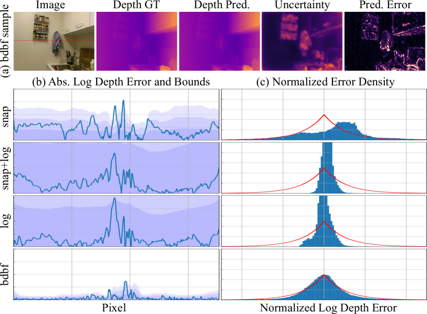
Figure 4: (a) Qualitative results of bdbf on one test image from NYU-V2. (b) Absolute log depth error (blue line) and $3b$ bounds (blue shades) for a single row of pixels (red line) from the image. (c) Normalized error density of the entire image compared to a unit Laplace distribution (red line). All axes are of the same scale within each column.

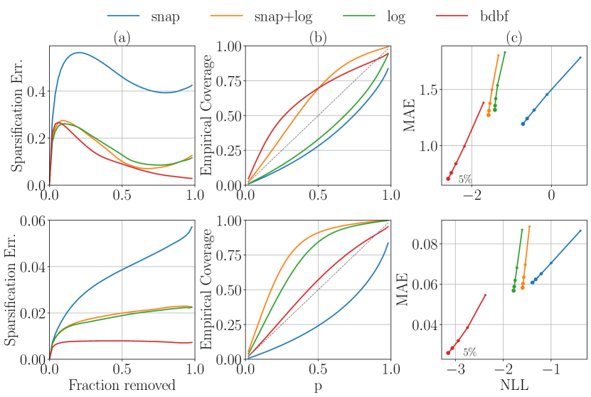
Figure 5: (a) Sparsification error, (b) calibration error and (c) sparsity change plots of NLL vs. MAE with 5% sparsity on VKITTI2 (top) and NYU-V2 (bottom). Sparsification and calibration plots are generated using 5% test sparsity. Sparsity change plots are generated with varying test sparsity from 5% to 1%.

Mid-density Depth Completion. In this setting, we train all methods with 5% sparsity. Table 2 shows quantitative results when testing on the same dataset under the same sparsity level. This is considered an in-distribution test. We see significant improvements of our method in almost all metrics. Figure 3 shows qualitative results of one sample from the VKITTI2 test set. Compared to others, bdbf not only predicts higher quality depths but also sharper uncertainties that closely match the true prediction errors. This indicates that the learned depth bases in ours is expressive for predicting both depth and uncertainty.

We take a closer look at one sample from the NYU-V2 test set in Figure 4 (a), by plotting the absolute prediction error in log space $e=|\mu-z|$ and uncertainty bound $b=\sigma/\sqrt{2}$ for one row of pixels in Figure 4 (b), and the normalized error density $\widetilde{e}=e/b$ on the entire image in Figure 4 (c). bdbf is the only method where the bound traces the general shape of the prediction error and whose normalized error density resembles that of a unit Laplace distribution. snap fails to capture the underlying error distribution. log and snap+log produce decent relative uncertainties (AUSE) but are not well-calibrated (AUCE). Figure 5 (a) (b) show sparsification error and calibration plots for the in-distribution test on both datasets, which are used to compute AUSE and AUCE respectively. We see that predictive method (log) performs similar to its ensemble variant snap+log and both are better than the pure ensemble method, snap. This is consistent with findings in [31, 55].

We also evaluate all methods under the effect of distributional (dataset) shift [53]. Here we mainly focus on the following two aspects: sparsity change and domain shift. For sparsity change within mid-density, we take models trained on 5% sparsity and test on varying sparsity level from 5% to 1%. Results are shown in Figure 5 (c). Note that these plots reflect how each method performs on two axes in terms of uncertainty estimation (NLL) and depth prediction (MAE), where better methods should reside closer to the lower left corner. We see that performance of all methods degrade in a similar manner with deceasing sparsity, which is largely due to the sparse depth scaffolding approach we choose. However, bdbf stands out with its 1% result better than the 5% results of its competitors. We refer the reader to our supplementary material for results on domain shift.

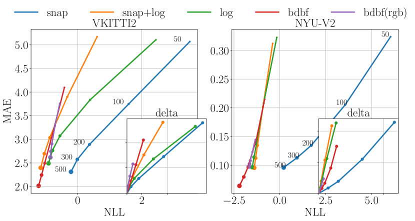
Figure 6: Sparsity change plots of all methods trained with 500 sparse depths and test with various sparsity from 500 to 50. The small subplots show how the performance of each method changes with decreasing sparsity w.r.t. the performance of their in-distribution test (500). Shorter lines indicate better sparsity-invariance.

Low-density Depth Completion. In this setting, we train all methods with 500 sparse points, which is roughly 0.5% sparsity given our image size. We also introduce a slight variation of our method bdbf(rgb) which only uses sparse depths at the fitting stage (not as network input). Because at very low sparsity levels (e.g. 50 points), the scaffolding method we use for depth interpolation [70] struggles to recover the scene structure which impacts the performance of all rgbd methods.

The top half of Table 3 shows the in-distribution test of all methods. Among the four rgbd methods, bdbf again outperforms the rest by a large margin. bdbf(rgb), despite not utilizing the rich information provided by the interpolated depths, performs on-par with the baselines. The real advantage of this approach is that it does not suffer from the artifacts caused by poor depth interpolation in the very low sparsity regime, which makes it sparsity-invariant. This claim is verified in Figure 6, which shows how each method’s performance deteriorates with decreasing sparsity. It is shown in the small subplots that bdbf(rgb) is able to maintain good performance even with as few as 50 points.

Finally, we test bdbf(rgb) with no sparse depths, which relies only on the shared prior to make a prediction. We ignore all rgbd methods because with nothing to interpolate the network outputs poor solutions. We thus only compare to another baseline log(rgb), which is trained for monocular depth prediction with NLL loss. Note that bdbf(rgb) and log(rgb) have exactly the same architecture (except for the last layer) and number of parameters. We see that bdbf(rgb) produces sharper depth than the baseline as shown in Figure 7. Quantitative results can be found in the last two rows of Table 3. The difference in performance of our method between two datasets is due to the distribution of the data: VKITTI2 contains mainly sequential driving videos, which gives a sharply peaked prior; whereas data from NYU-V2 are taken from a wide variety of scenes with different viewing angles, hence a less informative one. These results show that our learned depth bases and shared prior contain geometric information about the scene conditioned on the image and can be used under extreme conditions without catastrophic failure.

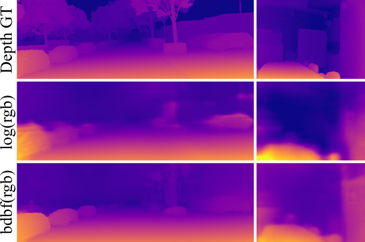
Figure 7: Qualitative results of our method tested with 0 sparse points. log(rgb) is trained as a monocular depth prediction network with NLL loss, which serves as a baseline. bdbf(rgb) is trained with 500 sparse depths.

Method	iRMSE	iMAE	RMSE	MAE
S2D [45]	2.80	1.21	814.73	249.95
Gansbeke [21]	2.19	0.93	772.87	215.02
DepthNormal[71]	2.42	1.13	777.05	235.17
DeepLiDAR [56]	2.56	1.15	758.38	226.50
FuseNet [9]	2.34	1.14	752.88	221.19
CSPN++ [10]	2.07	0.90	743.69	209.28
NLSPN [54]	1.99	0.84	741.68	199.59
GuideNet [65]	2.25	0.99	736.24	218.83
bdbf (ours)	2.37	0.89	900.38	216.44

Table 4: Comparison with selected methods on the official KITTI depth completion test set.

Method	MAE	RMSE	AUSE	AUCE	NLL
NCNN-L2 [16]	258.68	954.34	0.70	-	-
pNCNN [15]	283.41	1237.65	0.055	-	-
pNCNN-Exp	251.77	960.05	0.065	-	-
bdbf (ours)	206.70	876.76	0.057	0.23	-2.68

Table 5: Comparison with variations of pNCNN [15] on accuracy and uncertainty on the official KITTI validation set (with groundtruth). Note that pNCNN is unguided.

Further Comparisons. While our focus is on evaluating the quality of our uncertainty estimation scheme, we also evaluate depth completion performance for completeness. We trained our method with a ResNet34 encoder [27] and applied it to the KITTI depth completion benchmark with results shown in Table 4. We compare our relatively simple Bayesian filtering scheme to SOTA methods that utilize either iterative refinement [10, 54] or sub-networks with extra constraints [71, 56]. Our method compares favorably on all measures except RMSE and we observe that this difference is due to a small number of mis-attributed pixels near depth discontinuities and the use of L1 loss only. This suggests that these methods could be further improved by predicting initial depth and uncertainty estimates with our module.

We also compare with pNCNN [15] as it is the only work that provides a quantitative evaluation of predicted uncertainties for depth completion. Unfortunately, they only evaluate using a single metric, AUSE, which we argue cannot completely capture the true quality of the uncertainty estimate. Results are shown in Table 5, note that pNCNN is unguided and evaluation is done on the KITTI validation set, as groundtruth is required to compute uncertainty metrics.

5 Conclusions

In this paper, we extend Deep Basis Fitting for depth completion under a principled Bayesian framework that outputs uncertainty estimates alongside depth prediction. Compared to commonly used uncertainty estimation techniques, our integrated approach is able to produce better uncertainty estimates while being data- and compute-efficient. The benefit of being Bayesian is also demonstrated by the ability to handle very low-density sparse depths, a situation where the original DBF method struggles. Our work allows a depth completion network to be further integrated into robotics systems, where Bayesian sensor fusion is the dominant approach.

6 Network Architecture

The specific network architecture is of little importance to our approach, since all methods use exactly the same basis network, initialization and random seeds. Nevertheless, we list detailed architecture here for completeness.

We use the scaffolding approach detailed in [70] to interpolate sparse depths input. We then adopt an early fusion strategy where the interpolated depth map goes through a single convolution block (with normalization and nonlinear activation) with stride 2 to be merged with the first stage feature map of the image encoder. The fused feature map is then used as input to the subsequent stages of the encoder. The encoder is an ImageNet-pretrained MobileNet-v2 [58] which output a set of multi-scale feature maps $\{E_{i}\}$ at each stage with channels (16, 24, 32, 96, 320) in decreasing resolution. These feature maps except for the last one are then used as skip connection to the decoder, which eventually output another set of multi-scale features $\{D_{i}\}$ with channels (256, 192, 128, 64, 32) in increasing resolution. We keep the encoder essentially intact, while using ELU [12] activation throughout the decoder. This is due to the suggestion from [62], where they found a smooth activation function produces better quality uncertainty estimates. The decoder output $\{D_{i}\}$ are then used to generate the final multi-scale bases $\{\Phi_{i}\}$ with channels (2, 4, 8, 16, 32) in increase resolution. They are then upsampled (via bilinear interpolation) to the input image resolution and concatenated together [57]. This final 63-dimensional basis $\Phi$ (with a bias channel) is fed into either our proposed bdbf module, or a normal convolution to generate the latent prediction before the final activation function $g$.

7 Derivations

In this section, we provide derivation of equations given in the main paper, which roughly follows the same order of their original appearance.

7.1 Marginal Likelihood

The derivation of the full marginal likelihood function largely follows that from Chapter 3.5 in [4].

We start by writing the evidence function in the form

$$\begin{split}&p(\mathbf{z}|\alpha,\beta)\\ =&\int p(\mathbf{z}|\mathbf{w},\beta)p(\mathbf{w}|\alpha)\mathrm{d}\mathbf{w}\\ =&|\bm{\Sigma}_{0}|^{-1/2}\left(\frac{\beta}{2\pi}\right)^{\frac{N}{2}}\left(\frac{\alpha}{2\pi}\right)^{\frac{M}{2}}\int\exp\left\{-\frac{1}{2}E(\mathbf{w})\right\}\mathrm{d}\mathbf{w}\end{split}$$ (21)

where

$$E(\mathbf{w})=\beta\|\mathbf{z}-\bm{\Phi}\mathbf{w}\|^{2}+\alpha\|\mathbf{w}-\mathbf{m}_{0}\|^{2}_{\mathbf{\bm{\Sigma}_{0}}}$$ (22)

Completing the square over $\mathbf{w}$ we have

$$E(\mathbf{w})=E(\mathbf{m})+\|\mathbf{w}-\mathbf{m}\|^{2}_{\bm{\Sigma}}$$ (23)

The integral term is evaluated by

$$\begin{split}&\int\exp\left\{-\frac{1}{2}E(\mathbf{w})\right\}\mathrm{d}\mathbf{w}\\ =&\exp\left\{-\frac{1}{2}E(\mathbf{m})\right\}(2\pi)^{M/2}|\bm{\Sigma}|^{-1/2}\end{split}$$ (24)

We can then write the log marginal likelihood as

$$\begin{split}\ln p(\mathbf{z}|\alpha,\beta)&=\frac{1}{2}(N\ln\beta+M\ln\alpha-N\ln(2\pi)\\ &\qquad-E(\mathbf{m})+\ln|\bm{\Sigma}|-\ln|\bm{\Sigma}_{0}|)\end{split}$$ (25)

7.2 Normalized Estimation Error Squared (NEES)

NEES was originally used to indicate the performance of a filter [3], e.g. in a tracking application. It is defined as

$$\varepsilon_{k}=(\mathbf{x}_{k}-\hat{\mathbf{x}}_{k|k})^{\top}\mathbf{P}^{-1}_{k|k}(\mathbf{x}_{k}-\hat{\mathbf{x}}_{k|k})$$ (26)

where $\mathbf{x}$ is the true state vector, $\mathbf{P}$ is the state covariance matrix, and $(\hat{\cdot})_{k|k}$ denotes the estimated posterior at time $k$. It is also used in Simultaneous Localization and Mapping algorithms (SLAM) to measure filter consistency [2]. Specifically, the average NEES over N Monte Carlo runs is used. Under the assumption that the model is correct (approximately linear Gaussian), $\varepsilon_{k}$ is $\chi^{2}$ distributed with $\dim(\mathbf{x}_{k})$. Then the expected value of $\varepsilon_{k}$ should be

$$E[\varepsilon_{k}]=\dim(\mathbf{x}_{k})$$ (27)

For depth estimation, the state is the predicted depth at each pixel, which is one-dimensional. Therefore, we expect a consistent depth estimator to have an average NEES of 1.

NEES can also be extended to a Laplace distribution which is used in this work due to the choice of L1 loss. Given $z\sim\mathrm{Laplace}(\mu,b)$ and the fact that $\frac{2}{b}|z-\mu|\sim\chi^{2}(2)$, the expected NEES (with one degree of freedom) is

$$E[\varepsilon]=E\left[\left(\frac{z-\mu}{b}\right)^{2}\right]=1$$ (28)

7.3 Re-estimation Equations

Here we provide derivation of the re-estimation equations used in the EM step during inference [4]. In the E step, we compute the posterior distribution of $\mathbf{w}$ given the current estimation of the parameters $\alpha$ and $\beta$. In the M step, we maximize the expected complete-data log likelihood with respect to $\alpha$ and $\beta$ and re-iterate until convergence. The convergence criteria is met when the change in relative magnitude of $\beta$ is smaller than 1%.

The complete-data log likelihood function is given by

$$\ln p(\mathbf{z},\mathbf{w}|\alpha,\beta)=\ln p(\mathbf{z}|\mathbf{w},\beta)+\ln p(\mathbf{w}|\alpha)$$ (29)

with

$$p(\mathbf{z}|\mathbf{w},\beta) =\mathcal{N}(\mathbf{z}|\bm{\Phi}\mathbf{w},\beta^{-1}\mathbf{I})$$ (30)

$$p(\mathbf{w}|\alpha) =\mathcal{N}(\mathbf{w}|\mathbf{m}_{0},\alpha^{-1}\bm{\Sigma}_{0})$$ (31)

The expectation w.r.t. the posterior distribution of $\mathbf{w}$ is

$$\begin{split}&E[\ln p(\mathbf{z},\mathbf{w}|\alpha,\beta)]\\ =&\frac{M}{2}\ln\left(\frac{\alpha}{2\pi}\right)-\frac{1}{2}\ln|\bm{\Sigma}_{0}|-\frac{\alpha}{2}\mathbb{E}[\|\mathbf{w}-\mathbf{m}_{0}\|^{2}_{\bm{\Sigma}_{0}}]\\ +&\frac{N}{2}\ln\left(\frac{\beta}{2\pi}\right)-\frac{\beta}{2}\mathbb{E}[\|\mathbf{z}-\bm{\Phi}\mathbf{w}\|^{2}]\end{split}$$ (32)

Setting the derivatives with respect to $\alpha$ and $\beta$ to zero gives us the re-estimation equations.

$$\begin{split}\alpha&=\frac{M}{\mathbb{E}[\|\mathbf{w}-\mathbf{m}_{0}\|^{2}_{\bm{\Sigma}_{0}}]}\\ &=\frac{M}{\operatorname{tr}(\bm{\Sigma}_{0}^{-1}\bm{\Sigma})+\|\mathbf{m}-\mathbf{m}_{0}\|^{2}_{\bm{\Sigma}_{0}}}\end{split}$$ (33)

$$\begin{split}\beta&=\frac{N}{\mathbb{E}[\|\mathbf{z}-\bm{\Phi}\mathbf{w}\|^{2}]}\\ &=\frac{N}{\operatorname{tr}(\bm{\Phi}^{\top}\bm{\Phi}\bm{\Sigma})+\|\mathbf{z}-\bm{\Phi}\mathbf{m}\|^{2}}\end{split}$$ (34)

8 More Results

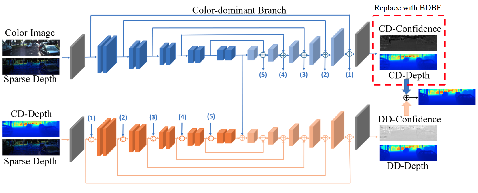
Figure 8: The backbone of PENet [28], which is called ENet, and our modification. Figure taken directly from the paper.

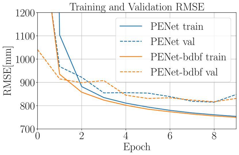
Figure 9: Training and validation RMSE of PENet and PENet-bdbf after training for 10 epochs on KITTI Depth Completion dataset.

8.1 Using BDBF as a General Component

Here we verify our claim that bdbf can be used as a general, drop-in, component in a depth completion network. The best published method on the KITTI depth completion benchmark at the time of this writing is PENet [28]. It has a fully-convolutional backbone called ENet that also ranks third on the associated leaderboard. For details of their approach, we refer the reader to the original paper [28]. We only discuss the minimal changes that we made to add bdbf.

Figure 8 shows the network architecture for ENet. The color-dominant (CD) branch uses a convolutional layer to predict CD-depth and CD-confidence. We simply replaced this convolutional layer with our bdbf module. However, we needed to normalize our variance prediction to conform to their notion of confidence. This was done by inverting the standard deviation and passing it through a Tanh nonlinearity to constrain the result to lie between 0 and 1. We then trained both versions for 10 epochs. Training and validation results are show in Figure 9. We see that by using bdbf, we achieve slightly better validation RMSE and faster convergence.

8.2 Inference Time

In table 6, we show inference time of all methods when running on an image of size $320\times 240$ with 5% sparsity levels. All ensemble methods (snap / snap+log) use 5 snapshots as described in the main paper. They take roughly 5$\times$ times longer for an inference pass compared to log, which is the fastest among all. For bdbf we use a maximum iteration of 8, but we observe convergence within 2 iterations for this particular density. bdbf is slower than log due to the need to solve a small linear system and the iterations required for EM, but it is has slower latency and smaller memory footprints compared to ensemble methods. Note that during inference, we move expensive computations in our method like Cholesky and LU decomposition from GPU to CPU and then move the results back. Since this is only done in evaluation mode, no back-propagation is needed and thus no computation graph broken. The time needed to transfer small tensors ($\dim(\mathbf{w})\times\dim(\mathbf{w})$) between host and device memory is negligible compared to carrying out those operations on GPU. Without these changes, bdbf runs as slow as snap.

Inference	snap	snap+log	log	dbf	bdbf
Time [ms]	68.84	66.17	16.68	21.84	23.97

Table 6: Inference time of all methods with 5% sparsity. Image resolution is $320\times 240$.

8.3 Estimator Consistency

Here we report average NEES scores for all methods on various datasets. NEES is not used as a metric in our evaluation since our method explicitly uses it for uncertainty calibration and would render the comparison unfair. We present it here only to show the efficacy of our uncertainty calibration scheme. Figure 10 and 11 show NEES of all methods under mid- and low- density with varying sparsity level. We see that our methods are the most consistent of all and remain relatively consistent even with sparsity change. Note that this consistency-based calibration can not be applied to other methods, because we did not observe the same amount of over- or under-confidence from them. While calibration of other baseline models is feasible, doing so would require extra data and thus not considered in this work.

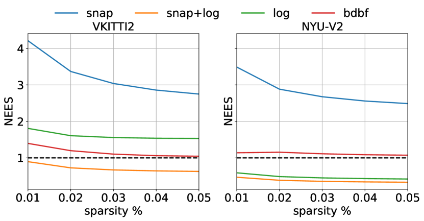
Figure 10: NEES scores for all methods with 5% sparsity. Closer to 1 (dashed black line) means more consistent.

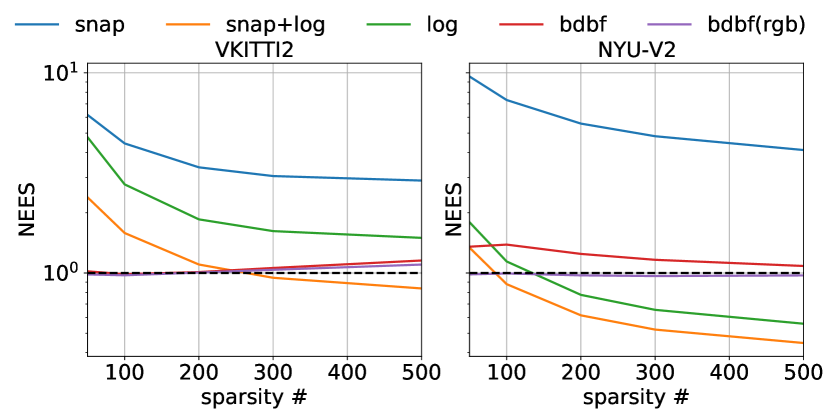
Figure 11: NEES scores for all methods with 500 sparse depths. Closer to 1 (dashed black line) means more consistent. Note the log scale on y-axis.

8.4 Shared Prior

Figure 12 supports our claim in the main paper about the assumption of a shared prior across samples. Here we show the weight histograms of two training sessions on different datasets (NYU-V2 and VKITTI2). We see that within each dataset, the weight distribution exhibits a fairly sharp peak. The small bump on the right side of each plot is formed by the bias term in the weights which reflects the average log depth of the dataset.

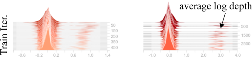
Figure 12: Tensorboard records of Weight histograms of two training sessions on NYU-V2 (left) and VKITTI2 (right).

8.5 Mid-density Depth Completion

	Trained and tested on KITTI (original)
Method	MAE	RMSE	$\delta_{1}$	AUSE	AUCE	NLL
snap	0.638	1.663	98.68	0.272	0.161	-1.298
snap+log	0.701	1.784	98.52	0.092	0.105	-1.605
log	0.899	2.022	98.44	0.109	0.133	-1.544
bdbf	0.364	1.682	98.74	0.060	0.100	-2.337
	Trained on VKITTI2 and tested on KITTI (shifted)
Method	MAE	RMSE	$\delta_{1}$	AUSE	AUCE	NLL
snap	1.296	2.549	92.03	0.876	0.161	-0.675
snap+log	0.853	2.245	97.69	0.134	0.117	-1.578
log	0.866	2.018	97.96	0.138	0.274	-0.755
bdbf	0.469	1.989	98.29	0.072	0.037	-2.381

Table 7: Quantitative results of all methods trained on KITTI and VKITTI with 5% sparsity and tested on KITTI.

Table 9 shows quantitative results of all methods trained with 5% sparsity and test on 5% and 1% sparsity. Here we also include comparison with dbf, where we simply ignore the prior during inference. We see that dbf and bdbf have perform similar due to the large amount of sparse depths, but bdbf still has the best performance overall. Figure 13 and 14 show some extra in-distribution samples of all methods from VKITTI2 and NYU-V2 respectively.

For domain shift, we take the same models that are trained on VKITTI2 and directly test on KITTI without any fine-tuning. The data distribution shift in this case manifests most notably in image quality as well as noise level and spatial distribution of sparse depths. Quantitative results are shown in Table 7, where we also list in-distribution test on KITTI for comparison. Most methods encounter performance drop in one or several metrics when tested under a slightly different domain. However bdbf achieve overall best results in both scenarios, with its performance under distributional shift better then some of the baselines in the original domain.

For more tests on distributional shift, we utilize the 15-deg and 30-deg sequences from VKITTI2. These sequences are variants of clone with the camera pointing at different angles. Table 8 shows quantitative results of all methods trained with 5% sparsity on VKITTI2 and test on these two sequences.

8.6 Low-density Depth Completion

Table 10 shows quantitative results of all methods trained with 500 sparse depths and test on 500 and 50 sparse depths. We choose 50 because it is smaller than the number of basis (63). This would previously fail with DBF, but BDBF have no problem dealing with any amount of sparse depths. Moreover, we suggest that when designing a system working under extremely low sparsity ($\leq$ 100 points) it is better to forgo the idea of a depth encoder altogether, because convolution is simply not designed for sparse data and interpolation schemes rarely work with only a few points.

Figure 15 and 17 show some extra in-distribution samples of all methods from VKITTI2 and NYU-V2 respectively.

Figure 16 shows more qualitative results of bdbf(rgb) and log(rgb) on VKITTI2 with no sparse depths.

	VKITTI2 (15-deg)
Method	MAE	RMSE	$\delta_{1}$	AUSE	AUCE	NLL
snap	1.164	3.161	95.67	0.445	0.172	-0.733
snap+log	1.206	3.260	95.43	0.131	0.103	-1.558
log	1.301	3.328	95.38	0.144	0.137	-1.347
bdbf	0.686	2.861	97.92	0.101	0.139	-2.618
	VKITTI2 (30-deg)
Method	MAE	RMSE	$\delta_{1}$	AUSE	AUCE	NLL
snap	1.084	3.009	95.39	0.428	0.175	-0.740
snap+log	1.139	3.106	95.10	0.128	0.087	-1.509
log	1.217	3.166	95.10	0.141	0.146	-1.251
bdbf	0.627	2.711	98.02	0.085	0.143	-2.676

Table 8: Quantitative results of all methods trained with 5% sparsity on VKITTI2 and test on 15-deg and 30-deg sequences from VKITTI2.

Trained with 5%			VKITTI2						NYU-V2
Input	Method	%	MAE	RMSE	$\delta_{1}$	AUSE	AUCE	NLL	MAE	RMSE	$\delta_{1}$	AUSE	AUCE	NLL
rgbd	snap	5%	1.192	3.267	95.59	0.445	0.170	-0.714	0.061	0.126	99.35	0.036	0.202	-1.390
rgbd	snap+log	5%	1.271	3.432	95.33	0.142	0.117	-1.582	0.058	0.123	99.32	0.018	0.256	-1.596
rgbd	log	5%	1.318	3.423	95.37	0.149	0.125	-1.421	0.057	0.121	99.34	0.018	0.210	-1.783
rgbd	dbf	5%	0.709	2.928	97.88	0.148	0.163	-2.489	0.026	0.083	99.64	0.007	0.054	-3.145
rgbd	bdbf	5%	0.703	2.925	97.88	0.110	0.136	-2.596	0.026	0.082	99.64	0.007	0.039	-3.151
rgbd	snap	1%	1.784	4.679	92.04	0.805	0.214	0.730	0.087	0.198	97.65	0.051	0.238	-0.387
rgbd	snap+log	1%	1.805	4.755	92.03	0.235	0.062	-1.333	0.089	0.211	97.35	0.025	0.202	-1.451
rgbd	log	1%	1.831	4.769	92.21	0.223	0.147	-1.168	0.087	0.214	97.31	0.023	0.157	-1.605
rgbd	dbf	1%	1.393	4.384	94.52	0.350	0.110	-1.670	0.055	0.155	98.45	0.016	0.072	-2.381
rgbd	bdbf	1%	1.382	4.372	94.53	0.271	0.082	-1.707	0.055	0.155	98.45	0.016	0.059	-2.374

Table 9: Quantitative results of all methods trained and tested with 5% and 1% sparsity on VKITTI2 and NYU-V2.

Trained with 500			VKITTI2						NYU-V2
Input	Method	#	MAE	RMSE	$\delta_{1}$	AUSE	AUCE	NLL	MAE	RMSE	$\delta_{1}$	AUSE	AUCE	NLL
rgbd	snap	500	2.312	5.403	90.14	0.459	0.229	-0.207	0.096	0.206	97.53	0.053	0.261	0.211
rgbd	snap+log	500	2.396	5.571	89.88	0.273	0.036	-1.150	0.095	0.213	97.44	0.025	0.205	-1.393
rgbd	log	500	2.492	5.800	89.13	0.299	0.095	-0.906	0.097	0.212	97.44	0.025	0.152	-1.502
rgbd	dbf	500	2.050	5.067	92.58	0.453	0.051	-1.175	0.065	0.168	98.45	0.020	0.055	-2.186
rgbd	bdbf	500	2.015	4.994	92.71	0.392	0.014	-1.215	0.064	0.166	98.46	0.021	0.030	-2.199
rgb	bdbf	500	2.569	5.642	88.67	0.481	0.015	-0.979	0.098	0.199	98.48	0.030	0.014	-1.689
rgbd	snap	50	5.069	9.326	66.48	1.696	0.327	3.495	0.324	0.605	78.89	0.136	0.376	6.036
rgbd	snap+log	50	5.173	9.401	65.91	1.180	0.188	0.608	0.312	0.593	80.55	0.084	0.052	-0.390
rgbd	log	50	5.107	9.433	66.52	1.114	0.275	2.439	0.323	0.599	80.49	0.088	0.134	-0.166
rgbd	bdbf	50	4.098	8.440	76.91	0.977	0.021	-0.411	0.215	0.446	88.63	0.081	0.026	-0.926
rgb	bdbf	50	3.725	7.786	80.67	0.701	0.012	-0.612	0.144	0.296	94.97	0.039	0.011	-1.338

Table 10: Quantitative results of all methods trained and tested with 500 and 50 sparse depths. rgbd under the input column indicates the basis network uses the sparse depths scaffolding approach from [70], whereas rgb uses color image as basis network input only.

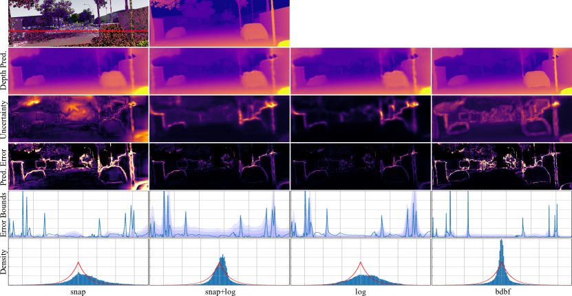
Figure 13: Sample qualitative results of all methods trained and test with 5% sparsity on VKITTI2. Colormaps scales are different for each methods to visualize details. Axes scales are same for all methods.

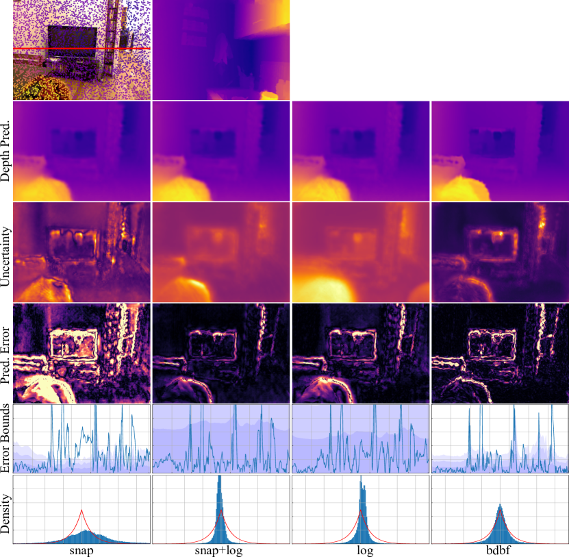
Figure 14: Sample qualitative results of all methods trained and test with 5% sparsity on NYU-V2. Colormaps scales are different for each methods to visualize details. Axes scales are same for all methods.

Figure 15: Sample qualitative results of all methods trained and test with 500 sparse points on VKITTI2. Colormaps scales are different for each methods to visualize details. Axes scales are same for all methods.

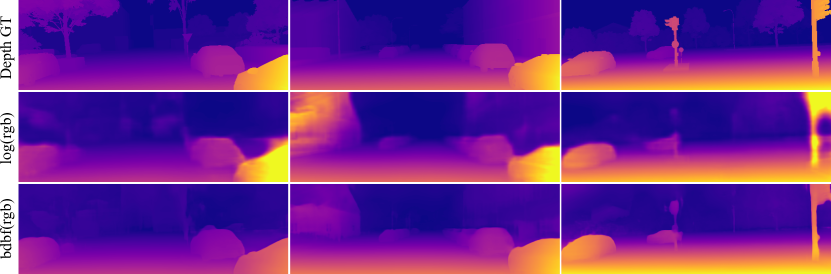
Figure 16: More qualitative results of our method tested with 0 sparse points. log(rgb) is trained as a monocular depth prediction network with NLL loss, which serves as a baseline. bdbf(rgb) is trained with 500 sparse depths.

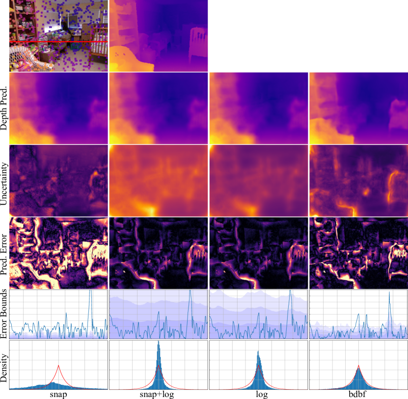
Figure 17: Sample qualitative results of all methods trained and test with 500 sparse points on NYU-V2. Colormaps scales are different for each methods to visualize details. Axes scales are same for all methods.

References

- [1] Oisin Mac Aodha, Ahmad Humayun, M. Pollefeys, and G. Brostow. Learning a confidence measure for optical flow. IEEE Transactions on Pattern Analysis and Machine Intelligence, 35:1107–1120, 2013.
- [2] T. Bailey, J. Nieto, J. Guivant, M. Stevens, and E. Nebot. Consistency of the ekf-slam algorithm. 2006 IEEE/RSJ International Conference on Intelligent Robots and Systems, pages 3562–3568, 2006.
- [3] Y. Bar-Shalom, X. Li, and T. Kirubarajan. Estimation with applications to tracking and navigation: Theory, algorithms and software. 2001.
- [4] C. M. Bishop. Pattern recognition and machine learning (information science and statistics). 2006.
- [5] Michael Bloesch, J. Czarnowski, Ronald Clark, S. Leutenegger, and A. Davison. Codeslam - learning a compact, optimisable representation for dense visual slam. 2018 IEEE/CVF Conference on Computer Vision and Pattern Recognition, pages 2560–2568, 2018.
- [6] Charles Blundell, Julien Cornebise, Koray Kavukcuoglu, and Daan Wierstra. Weight uncertainty in neural networks. arXiv preprint arXiv:1505.05424, 2015.
- [7] Yohann Cabon, Naila Murray, and Martin Humenberger. Virtual kitti 2, 2020.
- [8] J. Q. Candela, C. Rasmussen, Fabian H Sinz, O. Bousquet, and B. Schölkopf. Evaluating predictive uncertainty challenge. In MLCW, 2005.
- [9] Yuxiang Chen, Bin Yang, Ming Liang, and R. Urtasun. Learning joint 2d-3d representations for depth completion. 2019 IEEE/CVF International Conference on Computer Vision (ICCV), pages 10022–10031, 2019.
- [10] Xinjing Cheng, P. Wang, Chenye Guan, and Ruigang Yang. Cspn++: Learning context and resource aware convolutional spatial propagation networks for depth completion. ArXiv, abs/1911.05377, 2020.
- [11] Nathaniel Chodosh, Chaoyang Wang, and S. Lucey. Deep convolutional compressed sensing for lidar depth completion. ArXiv, abs/1803.08949, 2018.
- [12] Djork-Arné Clevert, Thomas Unterthiner, and S. Hochreiter. Fast and accurate deep network learning by exponential linear units (elus). CoRR, abs/1511.07289, 2016.
- [13] A. Dempster, N. Laird, and D. Rubin. Maximum likelihood from incomplete data via the em - algorithm plus discussions on the paper. 1977.
- [14] David Eigen, Christian Puhrsch, and Rob Fergus. Depth map prediction from a single image using a multi-scale deep network. In NIPS, 2014.
- [15] A. Eldesokey, M. Felsberg, Karl Holmquist, and M. Persson. Uncertainty-aware cnns for depth completion: Uncertainty from beginning to end. 2020 IEEE/CVF Conference on Computer Vision and Pattern Recognition (CVPR), pages 12011–12020, 2020.
- [16] A. Eldesokey, M. Felsberg, and F. Khan. Propagating confidences through cnns for sparse data regression. In BMVC, 2018.
- [17] David Ferstl, Christian Reinbacher, René Ranftl, M. Rüther, and H. Bischof. Image guided depth upsampling using anisotropic total generalized variation. 2013 IEEE International Conference on Computer Vision, pages 993–1000, 2013.
- [18] Adrien Gaidon, Qiao Wang, Yohann Cabon, and Eleonora Vig. Virtual worlds as proxy for multi-object tracking analysis. In Proceedings of the IEEE conference on Computer Vision and Pattern Recognition, pages 4340–4349, 2016.
- [19] Yarin Gal. Uncertainty in Deep Learning. PhD thesis, 2016.
- [20] Yarin Gal and Zoubin Ghahramani. Dropout as a bayesian approximation: Representing model uncertainty in deep learning. In ICML, 2016.
- [21] Wouter Van Gansbeke, D. Neven, Bert De Brabandere, and L. Gool. Sparse and noisy lidar completion with rgb guidance and uncertainty. 2019 16th International Conference on Machine Vision Applications (MVA), pages 1–6, 2019.
- [22] Jochen Gast and S. Roth. Lightweight probabilistic deep networks. 2018 IEEE/CVF Conference on Computer Vision and Pattern Recognition, pages 3369–3378, 2018.
- [23] T. Gneiting and A. Raftery. Strictly proper scoring rules, prediction, and estimation. Journal of the American Statistical Association, 102:359 – 378, 2007.
- [24] Alex Graves. Practical variational inference for neural networks. In Advances in neural information processing systems, pages 2348–2356, 2011.
- [25] Chuan Guo, Geoff Pleiss, Yu Sun, and Kilian Q. Weinberger. On calibration of modern neural networks. ArXiv, abs/1706.04599, 2017.
- [26] Fredrik K. Gustafsson, Martin Danelljan, and Thomas Bo Schön. Evaluating scalable bayesian deep learning methods for robust computer vision. 2020 IEEE/CVF Conference on Computer Vision and Pattern Recognition Workshops (CVPRW), pages 1289–1298, 2020.
- [27] Kaiming He, X. Zhang, Shaoqing Ren, and Jian Sun. Deep residual learning for image recognition. 2016 IEEE Conference on Computer Vision and Pattern Recognition (CVPR), pages 770–778, 2016.
- [28] Mu Hu, S. Wang, Bin Li, Shiyu Ning, L. Fan, and Xiaojin Gong. Penet: Towards precise and efficient image guided depth completion. ArXiv, abs/2103.00783, 2021.
- [29] Gao Huang, Y. Li, Geoff Pleiss, Zhuang Liu, J. Hopcroft, and K. Weinberger. Snapshot ensembles: Train 1, get m for free. ArXiv, abs/1704.00109, 2017.
- [30] P. Huber. Robust estimation of a location parameter. Annals of Mathematical Statistics, 35:492–518, 1964.
- [31] Eddy Ilg, Özgün Çiçek, Silvio Galesso, Aaron Klein, Osama Makansi, Frank Hutter, and Thomas Brox. Uncertainty estimates and multi-hypotheses networks for optical flow. In ECCV, 2018.
- [32] Michael I Jordan, Zoubin Ghahramani, Tommi S Jaakkola, and Lawrence K Saul. An introduction to variational methods for graphical models. Machine learning, 37(2):183–233, 1999.
- [33] Pasi Jylänki, Aapo Nummenmaa, and Aki Vehtari. Expectation propagation for neural networks with sparsity-promoting priors. The Journal of Machine Learning Research, 15(1):1849–1901, 2014.
- [34] Alex Kendall and Yarin Gal. What uncertainties do we need in bayesian deep learning for computer vision? In NIPS, 2017.
- [35] Diederik P. Kingma and Jimmy Ba. Adam: A method for stochastic optimization. CoRR, abs/1412.6980, 2015.
- [36] Armen Der Kiureghian and Ove D. Ditlevsen. Aleatory or epistemic? does it matter? 2009.
- [37] Agustinus Kristiadi, M. Hein, and Philipp Hennig. Being bayesian, even just a bit, fixes overconfidence in relu networks. ArXiv, abs/2002.10118, 2020.
- [38] A. Krizhevsky, Ilya Sutskever, and Geoffrey E. Hinton. Imagenet classification with deep convolutional neural networks. In CACM, 2017.
- [39] Balaji Lakshminarayanan, A. Pritzel, and Charles Blundell. Simple and scalable predictive uncertainty estimation using deep ensembles. In NIPS, 2017.
- [40] Ang Li, Zejian Yuan, Yonggen Ling, W. Chi, Shenghao Zhang, and C. Zhang. A multi-scale guided cascade hourglass network for depth completion. 2020 IEEE Winter Conference on Applications of Computer Vision (WACV), pages 32–40, 2020.
- [41] J. Liu and Xiaojin Gong. Guided depth enhancement via anisotropic diffusion. In PCM, 2013.
- [42] Wenxin Liu, D. Caruso, Eddy Ilg, Jing Dong, Anastasios I. Mourikis, Kostas Daniilidis, V. Kumar, and J. Engel. Tlio: Tight learned inertial odometry. IEEE Robotics and Automation Letters, 5:5653–5660, 2020.
- [43] Antonio Loquercio, Mattia Segù, and Davide Scaramuzza. A general framework for uncertainty estimation in deep learning. IEEE Robotics and Automation Letters, 5:3153–3160, 2020.
- [44] I. Loshchilov and F. Hutter. Sgdr: Stochastic gradient descent with warm restarts. In ICLR, 2017.
- [45] Fangchang Ma, G. Cavalheiro, and S. Karaman. Self-supervised sparse-to-dense: Self-supervised depth completion from lidar and monocular camera. 2019 International Conference on Robotics and Automation (ICRA), pages 3288–3295, 2019.
- [46] Fangchang Ma and S. Karaman. Sparse-to-dense: Depth prediction from sparse depth samples and a single image. 2018 IEEE International Conference on Robotics and Automation (ICRA), pages 1–8, 2018.
- [47] David J. C. MacKay. A practical bayesian framework for backpropagation networks. Neural Computation, 4:448–472, 1992.
- [48] Thomas Peter Minka. A family of algorithms for approximate Bayesian inference. PhD thesis, Massachusetts Institute of Technology, 2001.
- [49] Radford M. Neal. Bayesian Learning for Neural Networks. PhD thesis, CAN, 1995. AAINN02676.
- [50] D. Nix and A. Weigend. Estimating the mean and variance of the target probability distribution. Proceedings of 1994 IEEE International Conference on Neural Networks (ICNN’94), 1:55–60 vol.1, 1994.
- [51] Sebastian Ober and C. Rasmussen. Benchmarking the neural linear model for regression. ArXiv, abs/1912.08416, 2019.
- [52] Manfred Opper and Ole Winther. A bayesian approach to on-line learning. On-line learning in neural networks, pages 363–378, 1998.
- [53] Y. Ovadia, E. Fertig, J. Ren, Zachary Nado, D. Sculley, Sebastian Nowozin, Joshua V. Dillon, Balaji Lakshminarayanan, and Jasper Snoek. Can you trust your model’s uncertainty? evaluating predictive uncertainty under dataset shift. In NeurIPS, 2019.
- [54] Jinsun Park, Kyungdon Joo, Zhe Hu, Chi-Kuei Liu, and I. S. Kweon. Non-local spatial propagation network for depth completion. ArXiv, abs/2007.10042, 2020.
- [55] Matteo Poggi, Filippo Aleotti, Fabio Tosi, and Stefano Mattoccia. On the uncertainty of self-supervised monocular depth estimation. ArXiv, abs/2005.06209, 2020.
- [56] Jiaxiong Qiu, Zhaopeng Cui, Yinda Zhang, Xingdi Zhang, Shuaicheng C. Liu, Bing Zeng, and Marc Pollefeys. Deeplidar: Deep surface normal guided depth prediction for outdoor scene from sparse lidar data and single color image. ArXiv, abs/1812.00488, 2018.
- [57] Chao Qu, Ty Nguyen, and Camillo J. Taylor. Depth completion via deep basis fitting. 2020 IEEE Winter Conference on Applications of Computer Vision (WACV), pages 71–80, 2020.
- [58] Mark Sandler, A. Howard, Menglong Zhu, A. Zhmoginov, and Liang-Chieh Chen. Mobilenetv2: Inverted residuals and linear bottlenecks. 2018 IEEE/CVF Conference on Computer Vision and Pattern Recognition, pages 4510–4520, 2018.
- [59] K. Sartipi, T. Do, Tong Ke, Khiem Vuong, and S. Roumeliotis. Deep depth estimation from visual-inertial slam. 2020 IEEE/RSJ International Conference on Intelligent Robots and Systems (IROS), pages 10038–10045, 2020.
- [60] Nathan Silberman, Derek Hoiem, Pushmeet Kohli, and Rob Fergus. Indoor segmentation and support inference from rgbd images. In ECCV, 2012.
- [61] Edward Snelson, C. Rasmussen, and Zoubin Ghahramani. Warped gaussian processes. In NIPS, 2003.
- [62] Jasper Snoek, Oren Rippel, Kevin Swersky, Ryan Kiros, Nadathur Satish, N. Sundaram, Md. Mostofa Ali Patwary, Prabhat, and R. Adams. Scalable bayesian optimization using deep neural networks. In ICML, 2015.
- [63] Niko Sünderhauf, O. Brock, W. Scheirer, Raia Hadsell, D. Fox, J. Leitner, B. Upcroft, P. Abbeel, W. Burgard, Michael Milford, and P. Corke. The limits and potentials of deep learning for robotics. The International Journal of Robotics Research, 37:405 – 420, 2018.
- [64] Chengzhou Tang and P. Tan. Ba-net: Dense bundle adjustment networks. In ICLR, 2019.
- [65] J. Tang, F. Tian, W. Feng, J. Li, and Ping Tan. Learning guided convolutional network for depth completion. ArXiv, abs/1908.01238, 2019.
- [66] Sujay Thakur, Cooper Lorsung, Yaniv Yacoby, Finale Doshi-Velez, and Weiwei Pan. Learned uncertainty-aware (luna) bases for bayesian regression using multi-headed auxiliary networks. ArXiv, abs/2006.11695, 2020.
- [67] B. Triggs, P. McLauchlan, R. Hartley, and A. Fitzgibbon. Bundle adjustment - a modern synthesis. In Workshop on Vision Algorithms, 1999.
- [68] J. Uhrig, N. Schneider, Lukas Schneider, U. Franke, T. Brox, and A. Geiger. Sparsity invariant cnns. 2017 International Conference on 3D Vision (3DV), pages 11–20, 2017.
- [69] Tsun-Hsuan Wang, Fu-En Wang, Juan-Ting Lin, Yi-Hsuan Tsai, Wei-Chen Chiu, and M. Sun. Plug-and-play: Improve depth estimation via sparse data propagation. arXiv: Image and Video Processing, 2018.
- [70] Alex Wong, Xiaohan Fei, Stephanie Tsuei, and Stefano Soatto. Unsupervised depth completion from visual inertial odometry. IEEE Robotics and Automation Letters, 5:1899–1906, 2020.
- [71] Y. Xu, Xinge Zhu, Jianping Shi, Guofeng Zhang, H. Bao, and Hongsheng Li. Depth completion from sparse lidar data with depth-normal constraints. 2019 IEEE/CVF International Conference on Computer Vision (ICCV), pages 2811–2820, 2019.
- [72] Hongyang Xue, Shengming Zhang, and Deng Cai. Depth image inpainting: Improving low rank matrix completion with low gradient regularization. IEEE Transactions on Image Processing, 26:4311–4320, 2017.
- [73] Yanchao Yang, A. Wong, and Stefano Soatto. Dense depth posterior (ddp) from single image and sparse range. 2019 IEEE/CVF Conference on Computer Vision and Pattern Recognition (CVPR), pages 3348–3357, 2019.
- [74] Y. Zhang and T. Funkhouser. Deep depth completion of a single rgb-d image. 2018 IEEE/CVF Conference on Computer Vision and Pattern Recognition, pages 175–185, 2018.
- [75] Shanshan Zhao, M. Gong, Huan Fu, and Dacheng Tao. Adaptive context-aware multi-modal network for depth completion. ArXiv, abs/2008.10833, 2020.
- [76] Xingxing Zuo, N. Merrill, W. Li, Yiping Liu, Marc Pollefeys, and Guoquan Huang. Codevio: Visual-inertial odometry with learned optimizable dense depth. ArXiv, abs/2012.10133, 2020.