Exploiting Local Geometry for Feature and Graph Construction for Better 3D Point Cloud Processing with Graph Neural Networks

Abstract

We propose simple yet effective improvements in point representations and local neighborhood graph construction within the general framework of graph neural networks (GNNs) for 3D point cloud processing. As a first contribution, we propose to augment the vertex representations with important local geometric information of the points, followed by nonlinear projection using a MLP. As a second contribution, we propose to improve the graph construction for GNNs for 3D point clouds. The existing methods work with a $k$-NN based approach for constructing the local neighborhood graph. We argue that it might lead to reduction in coverage in case of dense sampling by sensors in some regions of the scene. The proposed methods aims to counter such problems and improve coverage in such cases. As the traditional GNNs were designed to work with general graphs, where vertices may have no geometric interpretations, we see both our proposals as augmenting the general graphs to incorporate the geometric nature of 3D point clouds. While being simple, we demonstrate with multiple challenging benchmarks, with relatively clean CAD models, as well as with real world noisy scans, that the proposed method achieves state of the art results on benchmarks for 3D classification (ModelNet40) , part segmentation (ShapeNet) and semantic segmentation (Stanford 3D Indoor Scenes Dataset). We also show that the proposed network achieves faster training convergence, i.e. $\sim 40\%$ less epochs for classification. The project details are available at https://siddharthsrivastava.github.io/publication/geomgcnn/

I Introduction

Significant progress has been made recently towards designing neural network architectures for directly processing unstructured 3D point clouds [1]. Since 3D point clouds are obtained as the native output from commonly available scanning sensors, the ability to process them and apply machine learning methods directly to them is interesting, and allows for many useful applications [2]. Like many other input modalities, both handcrafted and learning based methods are available for extracting meaningful information from 3D point clouds. The current state-of-the-art techniques for extracting such information are mostly based on deep neural networks.

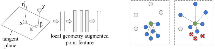
Figure 1: We propose two components which work within the framework of graph neural networks for 3D point cloud processing. First, we propose to augment the point representations, not just by point features (e.g. coordinates) but also with local geometric information such as the in and out plane distances $\alpha,\beta$ (shown in left), w.r.t. the tangent plane of point $\mathbf{x}$, to the nearby points, e.g. $\mathbf{y}$. We further propose to nonlinearly project the resulting feature with a small neural network. Second, we propose to construct the local neighborhood graph in a geometrically aware way. While in the usual $k$-NN based construction, the local graph can get biased towards a certain local neighborhood in the case of selective dense sampling, the proposed method aims to avoid that (shown in the two right blocks), by selecting the neighbors in a geometrically aware fashion. Best viewed in color.

As the point clouds are unordered, it is difficult to use CNNs with them. The popular ways of overcoming the problem of unstructured point clouds have been to either (i) voxelize them, e.g. [3] or (ii) learn a permutation invariant mapping, e.g. [4]. Point clouds can also be seen as graphs with potential edges defined between neighboring points. Therefore, utilizing graph neural networks (GNN) for processing point cloud data emerges as a natural choice. Most of the earlier GNN methods [5] considered the points in isolation, and did not explicitly utilize the information from local neighborhoods. While such local geometric information can be helpful for higher level tasks, these methods expected the network to learn the important intricacies directly from isolated points as inputs. However, the Dynamic EdgeConv network [6] showed that local geometric properties are important for learning feature representations from point clouds. They proposed to use the differences between the 3D points and their neighbors, which can be interpreted as a 3D direction vector, to encode the local structure. In addition, they converted the point cloud to a graph using a $k$-NN based construction, which is another way of encoding local geometric structure for use by the method. By doing this they were able to close the gap between GNN based methods and other state-of-the-art point cloud processing methods.

Along the lines of Dynamic EdgeConv, we believe that presenting more geometric information encoded in a task relevant way is important for the success of GNNs for point cloud processing. The generic graph networks [5] were designed to work with general graphs, e.g. citation networks, social network graphs etc. In such graphs there is no notion of geometric relations between vertices. However, point cloud data is inherently geometric and one could expect the performance to increase when the two natural properties of the point cloud data, i.e. graph like structure, and geometric information, are co-exploited. We see Dynamic EdgeConv work as a step along, and propose to go further in this direction.

We propose two novel, simple but extremely effective, components within the framework of general GNNs based on the intuitions above as shown in Figure 1. First, we propose to encode detailed local geometric information, inspired by traditional handcrafted 3D descriptors, about the points. Further, to convert the raw geometric information to a form which is easily exploited, we propose to use a multi layer perceptron network (MLP) to nonlinearly project the point features into another space. We then propose to present the projected representations as inputs to the graph network. This goes beyond the usual recommendation in previous works, where the possibility of adding more information about the point, e.g. color, depth, in addition to its 3D coordinates, has been often mentioned. We encode not only more information about the point, but also encode the information derived from the local neighborhood, around the point, as shown beneficial by previous works in handcrafted 3D descriptors. We also project such information nonlinearly to make it better exploitable by the GNN. While, in theory such information can be extracted by the neural network from 3D point coordinate inputs, we believe that presenting this information upfront allows the network to start from a better point, and even regularizes the learning.

Second, we propose a geometrically informed graph construction which goes beyond the usual $k$-NN based construction. We constrain the sequential selection of points to be added to a local graph based on their angles and distances with already selected points, while considering the point of interest as the center of reference. This increases the coverage of the local connectivity and especially addresses cases where the points might be very densely sampled in one neighborhood, while relatively sparsely sampled in another.

We show empirically that both the contributions, while being relatively simple, are significant and help improve the performance of the baseline GNN. We report results on multiple publicly available challenging benchmarks of point clouds including both CAD models and real world 3D scans.

The results on the real world datasets help us make the point that the local geometry extraction methods work despite the noise in real world scans.

In summary, the contributions of this work are:

• We propose to represent the vertices in a point cloud derived graph, corresponding to the 3D points, with geometric properties computed with respect to their local neighborhoods.

• We propose a geometrically informed construction of the local neighborhood graph, instead of using a naïve $k$-NN based initialization.

• We give extensive empirical results on five public benchmarks i.e. classification on ModelNet40 [7], part segmentation on ShapeNet [8] and semantic segmentation on ScanNet [9], S3DIS [10] and Paris-Lille-3D [11], reporting state-of-the-art results on three of them, while competing with both graph based as well as other neural networks for point cloud processing. We also give exhaustive ablation results and indicative qualitative results to fully validate the method.

II Related Works

Many tasks in 3D, such as classification and segmentation, can be solved by exploiting the local geometric structure of point clouds. In earlier efforts, handcrafted descriptors did this by encoding various properties of local regions in point clouds. The handcrafted descriptors, in general, fall into two categories. First are based on spatial distribution of the points, while the second directly utilize geometric properties of the points on surface.

Most of the handcrafted descriptors are based on finding a local reference frame which provides robustness to various types of transformations of the point cloud. Spin Image [12] uses in-plane and out-plane distance of neighborhood points within the support region of the keypoint to discretize the space and construct the descriptor. Local Surface Patches [13, 14] utilizes shape index [15] and angle between normals to accumulate points forming the final descriptor.

3D Binary Signatures [16] uses binary comparisons of geometrical properties in a local neighborhood. We refer the reader to Guo et al. [17] for a comprehensive survey of handcrafted 3D local descriptors.

Further, learning based methods have also been applied to obtain both local and global descriptors in 3D. Compact Geometric Features (CGF) [18] learns an embedding to a low dimensional space where the similar points are closer. DLAN [19] performs aggregation of local 3D features using deep neural network for the task of retrieval. DeepPoint3D [20] learns discriminative local descriptors by using deep metric learning.

While 3D local descriptors are still preferred for tasks such as point cloud registration, 3D deep networks trained for generating a global descriptor have provided state-of-the-art results on various classification, segmentation and retrieval benchmarks. The deep networks applied to these tasks are primarily based on volumetric representations (voxels, meshes, point clouds) and/or multi-view renderings of 3D shapes. We focus on techniques which directly process raw 3D point clouds as we work with them as well.

PointNet [4] directly processes 3D point clouds by aggregating information using a symmetric function. PointNet++ [21] applies hierarchical learning to PointNet to obtain geometrically more robust features. Kd-Net [22] constructs a network of kd-trees for parameter learning and sharing. PCNN [23], RS-CNN [24], LP-3DCNN [25], MinkowskiNet [26], FKAConv [27], PointASNL [28] propose modifications to convolution kernel or layers to produce features.

Recently, graph based neural networks have shown good performance on such unstructured data [29, 30, 31]. Dynamic Edge Convolutional Neural Network (DGCNN) [6] showed that by representing the local neighborhood of a point as a graph, it can achieve better performance than the previous techniques. Moreover, many previous works such as PointNet, PointNet++ become a special case with various Edge Convolution functions. LDGCNN [32] extends DGCNN by hierarchically linking features from the dynamic graphs in DGCNN. Authors in  [33, 34] propose modifications to kernels to capture geoemtric relationships between points. Our proposals are mainly within the purview of GNNs, however we extensively compare with most of the existing 3D point cloud based methods and show better results.

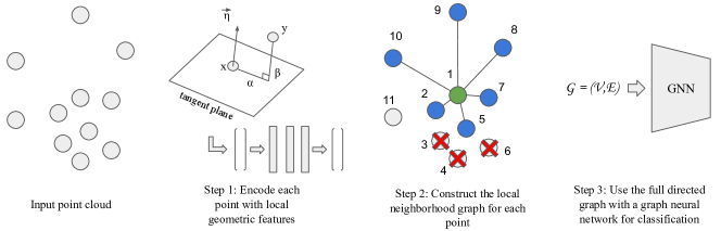
Figure 2: Illustration of of the proposed method. The input point cloud is processed point by point to generate an eventual graph, with vertices represented as real vectors and having directed edges denoting local neighborhoods. The representation includes local geometric properties of the points (which is relative to other points in their neighborhood), along with their coordinates. The graph formulation is geometrically aware and counters oversampling in some regions of the space. The finally constructed graph can then be used with a graph neural network for supervised learning, e.g. for classification and part segmentation. Best viewed in color.

III Approach

We are interested in processing a set $\mathbf{X}$, i.e. a point cloud, of 3D points. We follow the general graph neural network (GNN) based processing, where we work with a directed graph $\mathcal{G}=(\mathcal{V},\mathcal{E})$ with the points being the vertices $\mathcal{V}$ and the edges being potential connections between them. The vertices in $\mathcal{V}$ are represented by a $D$ dimensional feature vector, which is often just the 3D coordinate of the points, and the set of edges is constructed usually with a $k$-NN based graph construction algorithm. We now describe our two contributions pertaining to (i) the representation of the points using local geometric information and (ii) constructing the graph edges $\mathcal{E}$ with a geometrically constrained algorithm. Figure 2 gives an overall block diagram of our full system.

III-A Local Geometric Representation of Points

Majority of the GNN based previous works use a basic representations of points, i.e. their 3D coordinates, and feed that to the GNN to extract more complex interactions between neighboring points. Since GNNs, e.g. [5], were designed for general graphs which may not have any geometric properties, e.g. social network graphs, they do not have any explicit mechanism to encode geometry. More recent works on point cloud processing have started exploiting the geometric nature of 3D data more explicitly. As a specific case, EdgeConv [6] uses an edge function of the form

$h_{\boldsymbol{\Theta}}(\mathbf{x}_{i},\mathbf{x}_{j})=\bar{h}_{\boldsymbol{\Theta}}(\mathbf{x}_{i},\mathbf{x}_{j}-\mathbf{x}_{i}).$

where $\mathbf{x}_{i}$ is the point under consideration, and $\mathbf{x}_{j}$ is one of its neighbors. $h_{\boldsymbol{\Theta}}$ is a nonlinear function and $\boldsymbol{\Theta}$ is a set of learnable parameters. This function thus specifically uses a global description of the point, i.e. the point coordinates themselves, and a local description, which is the direction vector from the point to a nearby point. Providing such explicit local geometric description as input to the network layers helps EdgeConv outperform the baseline GNNs.

We go further in this direction and propose to use detailed geometric description of the local neighborhood of the point. Significant ingenuity was spent on the design of handcrafted 3D features (see [17] for a comparison), before deep neural networks became competitive for 3D point cloud processing. We take inspiration from such works in deriving the geometric descriptions of the points.

We include the following components in the representation of each point. As used in previous works, the first part is plain 3D coordinates of the point $(x,y,z)$, followed by the normal vector $\vec{\eta}=(\eta_{x},\eta_{y},\eta_{z})$ of the point. Then we take inspiration from the Spin Image descriptor [12] and add the in-plane and out-plane distances $\alpha,\beta$ w.r.t. the point. Finally, inspired by the Local Surface Patch Descriptor [13, 14], we include the shape index ($\gamma$) as well.

Hence, compared to a simple 3D coordinate based description of the points, we represent them with a 9D descriptor $\mathbf{p}=(x,y,z,\eta_{x},\eta_{y},\eta_{z},\alpha,\beta,\gamma)$ containing more local contextual geometric information. We then further pass this 9D descriptor through a small neural network $\phi(\cdot)$ to nonlinearly project it into another space which is more adapted to be used with the GNN. Finally, we pass the nonlinearly projected point representation $\phi(\mathbf{p})$ to the graph neural network.

While one can argue that such augmentation may be redundant as the GNN should be able to extract it out from 3D coordinates only, we postulate that providing these, successful handcrafted descriptor inspired and nonlinearly projected features, makes the job of the GNN easier. Another argument could be raised that these descriptors might be very task specific and hence might not be needed for a task of interest. In that case, we would argue that it should be possible for GNN to essentially ignore them by learning zero weights for weights/edges corresponding to these input units in the neural network. While this is a seemingly simple augmentation, we show empirically in Section IV that, in fact, adding such explicit geometric information does help the tasks of classification, part segmentation and semantic segmentation on challenging benchmarks, both based on clean CAD models of objects, as well as from real world noisy scans of indoor and outdoor spaces.

III-B Geometrically Constrained Neighborhood Graph Construction

Once the feature description is available, the next step is to define the directed edges between the points to fully construct the graph. We now detail our second contribution pertaining to the construction of the graph.

Previous methods construct the graphs using a $k$-NN scheme. Each point is considered, and directed edges are added from the point to its $k$ nearest neighbors. The graph thus constructed is given as input to the GNN which performs the final task.

A $k$-NN based graph construction scheme, while being intuitive and easy to implement, has an inherent problem. It is not robust to sampling frequency difference which can happen often in practice. Certain object may be densely sampled at some location in the scene, but the same object when placed at another location in the scene might only be sparsely sampled. Such scenarios can happen, for instance, in LiDAR based scanning, where the spatial sampling frequency is higher when the object is nearer to the sensor, but is lower when the object is farther. In such cases, $k$-NN may not cover the object sufficiently when the sampling density is higher, as all the $k$ nearest neighbors might be very close together, as shown in Figure 1 (center), and fall on the same subregion of the object. Hence, we propose a locality adaptive graph construction algorithm which promotes coverage in the local graph.

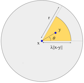
Figure 3: The local neighborhood graph construction constraints in 2D: Once a point $y$ is selected, for a point $x$, points from the yellow region, i.e. within an angle $\theta$ and a distance $\lambda\|x-y\|$ are discarded. This encourages coverage, and tackles densely sampled parts, in the local neighborhood graph. Best viewed in color.

The design of the graph construction is inspired by log-polar histograms which have been popular for many engineering applications. The main element is illustrated in Figure 3 in the case of 2D points. The construction iterates over each point one by one, and considers the sorted nearest neighbors of each point. However, instead of selecting the $k$-NN points, it greedily selects the neighbors as follows. At point $\mathbf{x}$, as soon as it selects a point $\mathbf{y}$, it removes all points in the region within an angle $\theta$ from the line $\mathbf{y}-\mathbf{x}$ with origin at $\mathbf{x}$, and with distance less than $\lambda\|\mathbf{x}-\mathbf{y}\|$, with both $\theta,\lambda$ being tunable hyper parameters, shown as the region marked in yellow in Figure 3. The simple intuition being that once a point from a local neighborhood has been sampled, we look for points which are sufficiently away from that local neighborhood. This ensures coverage in the local graph construction and improves robustness to sensor sampling frequency artefacts.

To illustrate the construction with a small toy example, we refer to Figure 2 (step 2). In the usual $k$-NN based graph construction, w.r.t. point $1$, the points which would have been selected would be $2,3,4,5,6,7$ (for $k=6$), which would concentrate the local neighborhood graph only on one region of the space. In contrast, with the proposed method, with appropriate $\theta,\gamma$, the selection of points $3,4,6$ can be avoided due to the presence of $2,5$, and the final six selected points would be $2,5,7,8,9,10$ which are well distributed in the space around the main point. Hence the problem of oversampling in some regions by the sensor can be avoided.

III-C Use with GNN

Given the above point descriptions, as well as graph edge constructions, we have a fully specified graph $\mathcal{G}=(\mathcal{V},\mathcal{E})$ derived from the point cloud data. This graph is general enough to be used with any GNN algorithm, while being specific to 3D point clouds as the vertex descriptions contain local geometric information, and the edges have been constructed in a geometrically constrained way. We stress here that while we give results with one specific choice of GNN in this paper, our graph can be used with any available GNN working on the input graph $\mathcal{G}$.

IV Experimental Results

We now give the results of the proposed methods on challenging benchmarks.

We denote the proposed methods as (i) ours (representation), when we incorporate the proposed local geometric representation, and (ii) ours (representation + graph) when we incorporate the proposed geometrically constrained graph construction as well.

IV-A Datasets and Experimental Setup

We evaluate the proposed method on the following datasets ModelNet40 [7], ShapeNet [8], ScanNet [9], Stanford Large-Scale 3D Indoor Spaces (S3DIS) scans [10], and Paris-Lille-3D (PL3D) [11]. We follow standard settings for training and evaluation on respective datasets. We use Dynamic Edge Convolutional network (DGCNN) [6] as the baseline network. Further, the input to the MLP is the 9D vector, it contains two FC layers with $18$ and $9$ units respectively.

IV-B Parametric Study

Table I gives the performances of the methods with different number of nearest neighbors. We see that for the baseline method, DGCNN with $k$-NN based graph construction, the performance initially increases with an increase in $k$ but then the drops a little, e.g. mean class accuracy goes from $88.0$ to $90.2$ for $k=5,20$, but then drops to $89.4$ for $k=40$. The authors in DGCNN [6] attributed this to the fact that for densities with large $k$ the Euclidean distance is not able to approximate the geodesic sufficiently well. However, for the proposed method the performance improves by a modest amount and does not drop, i.e. $89.8,93.1,93.8\%$ for $k=5,20,40$ respectively. This indicates that with explicit geometric information provided as input, the geometry is relatively better maintained cf. DGCNN. As the performance increase from $k=20$ to $k=40$ is modest for our method, we use $k=20$ as a good tradeoff between performance and time.

The values of $\theta=\frac{\pi}{6}$ and $\lambda=1.25$ were set based on validation experiments on a subset of the training and validation data for all experiments reported.

TABLE I: Results on ModelNet40 classification with varying number of nearest neighbors (#NN) for graph construction

# NN	DGCNN ($k$-NN)		ours (repr.) + $k$-NN		ours (graph)		ours (repr. + graph)
$k$	m-acc(%)	ov-acc(%)	m-acc(%)	ov-acc(%)	m-acc(%)	ov-acc(%)	m-acc(%)	ov-acc(%)
5	88.0	90.5	88.9	91.1	88.3	90.8	89.8	91.9
10	88.9	91.4	90.1	92.4	89.2	92.6	91.6	93.9
20	90.2	92.9	92.0	95.1	90.8	94.4	93.1	95.9
40	89.4	92.4	91.4	94.6	91.2	95.1	93.8	96.6

TABLE II: Comparison with state of the art methods on ModelNet40 classification and ShapeNet part segmentation datasets.

Method	ModelNet40		ShapeNet
	m-acc(%)	ov-acc(%)	mIoU(%)
PointNet [4]	86.0	89.2	83.7
PointNet++ [21]	-	90.7	85.1
Kd-net [22]	-	90.6	82.3
DensePoint [35]	-	93.2	86.4
LP-3DCNN [25]	-	92.1	-
DGCNN [6]	90.2	92.9	85.2
DGCNN (2048 pts) [6]	90.7	93.5	-
LDGCNN [32]	90.3	92.9	85.1
KPConv-rigid [36]	-	92.9	86.2
KPConv-deform [36]	-	92.7	86.4
GSN [37]	-	92.9	-
GSN (2048 pts) [37]	-	93.3	-
LS [38]	-	-	88.8
PointASNL [28]	-	93.2	-
SPH3D-GCN (2048 pts)  [33]	88.5	91.4	86.8
FKAConv [27]	89.9	92.5	-
FKAConv (2048 pts) [27]	89.7	92.5	85.7
ConvPoint [39]	88.5	91.8	85.8
ConvPoint (2048 pts) [39]	89.6	92.5	-
Ours (repr.)	92.0	95.1	87.4
Ours (repr. + graph)	93.1	95.9	89.1
Ours (repr. + graph) - 2048 pts	94.1	96.9	-

IV-C Comparison with state of the art

Classification on ModelNet40. The classification results on the ModelNet40 datasets are shown in Table II with comparison against methods based on 3D input. In the last block the first two rows of our method are with $1024$ points while the third (last) is with $2048$ points. Our full method achieves the best results, e.g. $95.9\%$ overall class accuracy, compared to many recent competitive methods such as PointASNL ($93.2\%$), RS-CNN ($93.6\%$) and the baseline DGCNN ($92.9\%$). We also see that our method improves more when the point sampling is increased from $1024$ to $2048$ with mean accuracy going from $93.1\%$ to $94.1\%$, cf. DGCNN $90.2\%$ to $90.7\%$ for the same settings.

ShapeNet Part Segmentation. Table II (Column 4) shows results on ShapeNet part segmentation. Similar to the classification case, we achieve higher results than many recent methods. Our representation only method achieves $87.4\%$ mIoU cf. $85.2\%$ of DGCNN [6]. While our full, representation and graph construction based method achieves $89.1\%$ which is higher than recently proposed learning to segment (LS) by $0.3\%$. However, LS projects the 3D points to 2D images and uses U-Net segmentation, while the proposed method directly computes the part labels on 3D points.

Semantic Segmentation. Table III show results of semantic segmentation on ScanNet, Stanford Indoor Spaces Dataset (S3DIS) and Paris-Lille-3D datasets (PL3D). On S3DIS dataset, we outperform all the compared methods w.r.t. mIoU and overall accuracy (ov-acc) on Area-5 protocol and w.r.t. overall accuracy on k-fold evaluation protocol. Further, we also outperform other methods w.r.t. overall accuracy on PL3D dataset. We outperform the next best method on PL3D (KPConv-deform, ConvPoint) by $2.6\%$ on mIoU while lag behind FKAConv by $4.2\%$, however, we outperform FKAConv on S3DIS (k-fold) by $1.7\%$ w.r.t. mIoU. On ScanNet we achieve an mIoU of $72.4\%$ lagging behind MinkowskiNet ($73.6\%$) and Virtual MVFusion ($74.6\%$), however, we outperform these methods on S3DIS by $\sim 4\%$.

Overall, we observe that our method consistently provides results amongst top-$3$ methods on all the compared benchmarks, demonstrating the robustness of the proposed modifications to datasets with significant noise e.g. ScanNet and well defined CAD models e.g. ModelNet40.

TABLE III: Comparison with state of the art methods for 3D scene segmentation on Scannet v2, Stanford 3D Indoor Spaces (S3DIS) and Paris-Lille-3D (PL3D) datasets.

Method	Scannet	S3DIS (k-fold)		S3DIS (Area 5)		PL3D
	mIoU	mIoU	ov-acc	mIoU	ov-acc	mIoU	ov-acc
PointNet [4]	-	47.6	78.6	41.1	-	40.2	93.9
PointNet++ [21]	33.9	54.5	81.0	-	-	36.1	88.7
PointCNN [40]	45.8	65.4	88.1	57.3	85.9	65.4	-
KPConv-rigid [36]	68.6	69.6	-	65.4	-	72.3	-
KPConv-deform [36]	68.4	70.6	-	67.1	-	75.9	-
DGCNN [6]	-	56.1	84.1	-	-	62.5	97.0
MinkowskiNet [26]	73.6	-	-	65.4	-	-	-
HDGCNN [31]	-	66.9	-	59.3	-	68.3	-
DPC [41]	59.2	-	-	61.3	86.8	-	-
Virtual MVFusion [42]	74.6	-	-	65.3	-	-	-
JSENet [43]	69.9	-	-	67.7	-	-	-
FusionNet [44]	68.8	-	-	65.38	-	-	-
DCMNet [45]	65.8	69.7	-	64.0	-	-	-
PointASNL [28]	63.0	68.7	-	-	-	-	-
SPH3D-GCN [33]	61.0	68.9	88.6	59.5	87.7	-	-
SegGCN [34]	58.9	68.5	87.8	63.6	88.2	-	-
ResGCN-28 [29]	-	60.0	85.9	-	-	-	-
FKAConv [27]	-	68.4	-	-	-	82.7	-
ConvPoint [39]	-	69.2	88.8	-	-	75.9	-
Ours (repr.+graph)	72.4	70.1	89.8	69.4	89.4	78.5	98.0
RANK	3	2	1	1	1	2	1

IV-D Qualitative Results

Figure 4 shows semantic segmentation results on S3DIS. In general, we observe that the proposed technique provides closer to ground-truth segmentation especially at the boundaries. In first row, we observe that the structures on the wall are better constructed by the proposed method as compared to DGCNN especially around the edges. In the box at center, we observe that the proposed method marks the points on the wall behind the table correctly while DGCNN incorrectly labels them as wall. Similarly, in second row, the labels in the box at top are closer to the ground truth with a clear separation from the wall. In the bottom box, we observe that the points on the table are clearly labelled by our method while DGCNN labels many points as walls. These results indicate that the proposed method is robust in narrow regions and on fine structures due to the explicit introduction of geometrical features to GCNN.

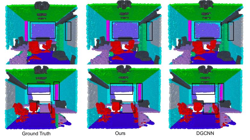
Figure 4: Qualitative results on S3DIS dataset, notice the fine structures captured by our method and missed by DGCNN, in the annotated black boxes. Best viewed zoomed in color.

TABLE IV: Ablation studies on impact of various components of the proposed method.

			ModelNet40		ShapeNet	S3DIS
$\alpha,\beta$	$\gamma$	graph	m-acc	ov-acc	mIoU	mIoU	ov-acc
$\times$	$\times$	$\times$	90.2	92.9	85.2	56.1	84.1
✓	$\times$	$\times$	90.8	93.4	86.1	57.8	84.7
$\times$	✓	$\times$	90.7	93.8	85.9	57.8	85.1
$\times$	$\times$	✓	90.8	94.4	86.2	59.4	86.6
✓	$\times$	✓	92.1	95.1	87.1	61.2	87.4
$\times$	✓	✓	91.8	94.9	86.8	62.1	87.4
✓	✓	$\times$	92.0	94.0	86.6	65.5	88.1
✓	✓	✓	93.1	95.9	89.1	69.4	89.4

IV-E Ablation Experiments

We perform ablation experiments to give the complete results with and without including the different components of the proposed method.

For ablation on absence of various local features, we only set the corresponding elements of the input vector to the MLP and train the projection MLP as usual.

Ablation on Classification. In Table IV columns 4 and 5, starting from a baseline of $92.9\%$ overall accuracy, we see that the local geometric features help individually, but their combination is better at $94.9\%$. Similarly, the graph construction method gives $94.4\%$ alone but improves with each of the geometric features added, and performance is best when all the features as well as graph construction are used together, at $95.9\%$.

Ablation on Part Segmentation. In Table IV column 6, we see similar trends as in the classification case, where each of the geometric features contribute ($86.1\%,85.9\%$), the graph construction helps when used alone ($86.2\%$), and the full combination achieves the best performance at $89.1\%$ mIoU, cf. the baseline at $85.2\%$ mIoU.

Ablation on Semantic Segmentation. In Table IV columns 7 and 8, we observe that with the graph construction only the mIoU increases from $56.1\%$ to $59.4\%$ while it increases to $65.5\%$ with only the combination of local features. However, the full combination provides the best performance at mIoU of $69.4\%$ and overall accuracy of $89.4\%$.

TABLE V: Ablation study on the training convergence of models

		ModelNet40		ShapeNet		S3DIS
$\alpha,\beta,\gamma$	graph	tr. epochs	frac.	tr. epochs	frac.	tr. epochs	frac.
$\times$	$\times$	233	1.00	190	1.00	258	1.00
✓	$\times$	205	0.87	174	0.91	243	0.94
$\times$	✓	164	0.70	151	0.79	215	0.83
✓	✓	139	0.60	133	0.70	191	0.73

Ablation on Model Convergence The number of epochs required for the different models to converge are shown in Table V. We observe that using the proposed geometric representation results in reduction by $13\%$, $9\%$ and $6\%$ epochs for classification, part segmentation and semantic segmentation respectively. With the proposed geometrically aware graph construction, we observe a reduction of $30\%$ for classification, $21\%$ for part segmentation and $17\%$ for semantic segmentation. Hence, providing a geometrically refined local connectivity information to the graph results in significant reduction in the number of epochs required by the network. Finally, the combination of the proposed geometric representation and the proposed graph construction results in a reduction of $40\%,30\%,27\%$ epochs required for the tasks respectively.

The actual training time required to train our full method on ModelNet40 is $3.2$ hours as compared to $5$ hours required by DGCNN, providing a training speed-up of nearly $36\%$, which is similar to the epoch reduction of $40\%$, i.e. less epochs translate directly into reduction in training time.

Ablation on MLP. With only 3D coordinates as input to the MLP, the m-acc on ModelNet40 is $90.9\%$ cf. $90.2\%$ (DGCNN). With 9D vector as a direct input without MLP to DGCNN, the m-acc is $91.1\%$ cf. $92.0\%$ with MLP (Table II, Ours(repr.)). This shows that MLP is able to extract a robust geometric representation in the feature space.

V Conclusion

We proposed two simple but important contributions, to be used within the framework of graph neural networks (GNN) for point cloud processing, on (i) representation of points using local geometric properties, and (ii) construction of the neighborhood graph using geometric constraints to improve coverage. We also reported highly competitive results, better than many recent state-of-the-art methods on both synthetic and real-world datsets showing robustness of the proposed approach to noisy data. Our work highlights the fact that the current generation of GNN based methods, for 3D point cloud processing, are not able to fully capture the local geometric information, and hence benefit from having that as input explicitly. Further, recently Liu et al. [46] showed that, the local aggregation operators used in various point cloud processing techniques, if carefully tuned, provide similar performances. Parida et al. [47] showed that using region/point based properties from echoes or type of material can help in learning more robust representations. Therefore, the proposed modifications, with explicit prior on geometry, can be extended to other point cloud based deep networks and potentially motivate future works with simpler and more efficient networks for processing point clouds.

References

- [1] A. Ioannidou, E. Chatzilari, S. Nikolopoulos, and I. Kompatsiaris, “Deep learning advances in computer vision with 3d data: A survey,” ACM Computing Surveys (CSUR), vol. 50, no. 2, p. 20, 2017.
- [2] W. Liu, J. Sun, W. Li, T. Hu, and P. Wang, “Deep learning on point clouds and its application: A survey,” Sensors, vol. 19, no. 19, p. 4188, 2019.
- [3] D. Maturana and S. Scherer, “Voxnet: A 3d convolutional neural network for real-time object recognition,” in Intelligent Robots and Systems (IROS), 2015 IEEE/RSJ International Conference on. IEEE, 2015, pp. 922–928.
- [4] C. R. Qi, H. Su, K. Mo, and L. J. Guibas, “Pointnet: Deep learning on point sets for 3d classification and segmentation,” Proceedings of the IEEE conference on computer vision and pattern recognition, 2017.
- [5] Z. Wu, S. Pan, F. Chen, G. Long, C. Zhang, and P. S. Yu, “A comprehensive survey on graph neural networks,” IEEE Transactions on Neural Networks and Learning Systems, 2020.
- [6] Y. Wang, Y. Sun, Z. Liu, S. E. Sarma, M. M. Bronstein, and J. M. Solomon, “Dynamic graph cnn for learning on point clouds,” ACM Transactions on Graphics (TOG), vol. 38, no. 5, p. 146, 2019.
- [7] Z. Wu, S. Song, A. Khosla, F. Yu, L. Zhang, X. Tang, and J. Xiao, “3d shapenets: A deep representation for volumetric shapes,” in Proceedings of the IEEE Conference on Computer Vision and Pattern Recognition, 2015, pp. 1912–1920.
- [8] L. Yi, V. G. Kim, D. Ceylan, I. Shen, M. Yan, H. Su, C. Lu, Q. Huang, A. Sheffer, L. Guibas, et al., “A scalable active framework for region annotation in 3d shape collections,” ACM Transactions on Graphics (TOG), vol. 35, no. 6, p. 210, 2016.
- [9] A. Dai, A. X. Chang, M. Savva, M. Halber, T. Funkhouser, and M. Nießner, “Scannet: Richly-annotated 3d reconstructions of indoor scenes,” in Proceedings of the IEEE Conference on Computer Vision and Pattern Recognition, 2017, pp. 5828–5839.
- [10] I. Armeni, O. Sener, A. R. Zamir, H. Jiang, I. Brilakis, M. Fischer, and S. Savarese, “3d semantic parsing of large-scale indoor spaces,” in Proceedings of the IEEE Conference on Computer Vision and Pattern Recognition, 2016, pp. 1534–1543.
- [11] X. Roynard, J.-E. Deschaud, and F. Goulette, “Paris-lille-3d: A large and high-quality ground-truth urban point cloud dataset for automatic segmentation and classification,” The International Journal of Robotics Research, vol. 37, no. 6, pp. 545–557, 2018.
- [12] A. E. Johnson and M. Hebert, “Surface matching for object recognition in complex three-dimensional scenes,” Image and Vision Computing, vol. 16, no. 9-10, pp. 635–651, 1998.
- [13] H. Chen and B. Bhanu, “3d free-form object recognition in range images using local surface patches,” Pattern Recognition Letters, vol. 28, no. 10, pp. 1252–1262, 2007.
- [14] ——, “Human ear recognition in 3d,” IEEE Transactions on Pattern Analysis and Machine Intelligence, vol. 29, no. 4, pp. 718–737, 2007.
- [15] J. J. Koenderink and A. J. Van Doorn, “Surface shape and curvature scales,” Image and vision computing, vol. 10, no. 8, pp. 557–564, 1992.
- [16] S. Srivastava and B. Lall, “3d binary signatures,” in Proceedings of the Tenth Indian Conference on Computer Vision, Graphics and Image Processing. ACM, 2016, p. 77.
- [17] Y. Guo, M. Bennamoun, F. Sohel, M. Lu, J. Wan, and N. M. Kwok, “A comprehensive performance evaluation of 3d local feature descriptors,” International Journal of Computer Vision, vol. 116, no. 1, pp. 66–89, 2016.
- [18] M. Khoury, Q.-Y. Zhou, and V. Koltun, “Learning compact geometric features,” Proceedings of the IEEE International Conference on Computer Vision, 2017.
- [19] T. Furuya and R. Ohbuchi, “Deep aggregation of local 3d geometric features for 3d model retrieval.” in BMVC, 2016.
- [20] S. Srivastava and B. Lall, “Deeppoint3d: Learning discriminative local descriptors using deep metric learning on 3d point clouds,” Pattern Recognition Letters, 2019.
- [21] C. R. Qi, L. Yi, H. Su, and L. J. Guibas, “Pointnet++: Deep hierarchical feature learning on point sets in a metric space,” Advances in neural information processing systems, 2017.
- [22] R. Klokov and V. Lempitsky, “Escape from cells: Deep kd-networks for the recognition of 3d point cloud models,” Proceedings of the IEEE International Conference on Computer Vision, 2017.
- [23] M. Atzmon, H. Maron, and Y. Lipman, “Point convolutional neural networks by extension operators,” ACM Transactions on Graphics, 2018.
- [24] Y. Liu, B. Fan, S. Xiang, and C. Pan, “Relation-shape convolutional neural network for point cloud analysis,” in Proceedings of the IEEE Conference on Computer Vision and Pattern Recognition, 2019, pp. 8895–8904.
- [25] S. Kumawat and S. Raman, “Lp-3dcnn: Unveiling local phase in 3d convolutional neural networks,” in Proceedings of the IEEE Conference on Computer Vision and Pattern Recognition, 2019, pp. 4903–4912.
- [26] C. Choy et al., “4d spatio-temporal convnets: Minkowski convolutional neural networks,” in Proceedings of the IEEE Conference on Computer Vision and Pattern Recognition, 2019, pp. 3075–3084.
- [27] A. Boulch et al., “FKAConv: Feature-Kernel Alignment for Point Cloud Convolution,” arXiv preprint arXiv:2004.04462, 2020.
- [28] X. Yan, C. Zheng, Z. Li, S. Wang, and S. Cui, “Pointasnl: Robust point clouds processing using nonlocal neural networks with adaptive sampling,” in Proceedings of the IEEE/CVF Conference on Computer Vision and Pattern Recognition, 2020, pp. 5589–5598.
- [29] G. Li, M. Muller, A. Thabet, and B. Ghanem, “Deepgcns: Can gcns go as deep as cnns?” in Proceedings of the IEEE International Conference on Computer Vision, 2019, pp. 9267–9276.
- [30] L. Wang, Y. Huang, Y. Hou, S. Zhang, and J. Shan, “Graph attention convolution for point cloud semantic segmentation,” in Proceedings of the IEEE Conference on Computer Vision and Pattern Recognition, 2019, pp. 10 296–10 305.
- [31] Z. Liang, M. Yang, L. Deng, C. Wang, and B. Wang, “Hierarchical depthwise graph convolutional neural network for 3d semantic segmentation of point clouds,” in 2019 International Conference on Robotics and Automation (ICRA). IEEE, 2019, pp. 8152–8158.
- [32] K. Zhang, M. Hao, J. Wang, C. W. de Silva, and C. Fu, “Linked dynamic graph cnn: Learning on point cloud via linking hierarchical features,” arXiv preprint arXiv:1904.10014, 2019.
- [33] H. Lei, N. Akhtar, and A. Mian, “Spherical kernel for efficient graph convolution on 3d point clouds,” IEEE Transactions on Pattern Analysis and Machine Intelligence, 2020.
- [34] ——, “Seggcn: Efficient 3d point cloud segmentation with fuzzy spherical kernel,” in Proceedings of the IEEE/CVF Conference on Computer Vision and Pattern Recognition, 2020, pp. 11 611–11 620.
- [35] Y. Zhao, T. Birdal, H. Deng, and F. Tombari, “3d point capsule networks,” in Proceedings of the IEEE Conference on Computer Vision and Pattern Recognition, 2019, pp. 1009–1018.
- [36] H. Thomas, C. R. Qi, J.-E. Deschaud, B. Marcotegui, F. Goulette, and L. J. Guibas, “Kpconv: Flexible and deformable convolution for point clouds,” in Proceedings of the IEEE International Conference on Computer Vision, 2019, pp. 6411–6420.
- [37] M. Xu, Z. Zhou, and Y. Qiao, “Geometry sharing network for 3d point cloud classification and segmentation.” in AAAI, 2020, pp. 12 500–12 507.
- [38] Y. Lyu, X. Huang, and Z. Zhang, “Learning to segment 3d point clouds in 2d image space,” in Proceedings of the IEEE/CVF Conference on Computer Vision and Pattern Recognition, 2020, pp. 12 255–12 264.
- [39] A. Boulch, “Convpoint: Continuous convolutions for point cloud processing,” Computers & Graphics, 2020.
- [40] Y. Li, R. Bu, M. Sun, W. Wu, X. Di, and B. Chen, “Pointcnn: Convolution on x-transformed points,” in Advances in Neural Information Processing Systems, 2018, pp. 820–830.
- [41] F. Engelmann et al., “Dilated point convolutions: On the receptive field of point convolutions,” ICRA, 2019.
- [42] A. Kundu, X. Yin, A. Fathi, D. Ross, B. Brewington, T. Funkhouser, and C. Pantofaru, “Virtual multi-view fusion for 3d semantic segmentation,” ECCV, 2020.
- [43] Z. Hu, M. Zhen, X. Bai, H. Fu, and C.-l. Tai, “Jsenet: Joint semantic segmentation and edge detection network for 3d point clouds,” ECCV, 2020.
- [44] F. Zhang, J. Fang, B. Wah, and P. Torr, “Deep fusionnet for point cloud semantic segmentation,” ECCV, 2020.
- [45] J. Schult, F. Engelmann, T. Kontogianni, and B. Leibe, “Dualconvmesh-net: Joint geodesic and euclidean convolutions on 3d meshes,” in Proceedings of the IEEE/CVF Conference on Computer Vision and Pattern Recognition, 2020, pp. 8612–8622.
- [46] Z. Liu, H. Hu, Y. Cao, Z. Zhang, and X. Tong, “A closer look at local aggregation operators in point cloud analysis,” ECCV, 2020.
- [47] K. K. Parida, S. Srivastava, and G. Sharma, “Beyond image to depth: Improving depth prediction using echoes,” in CVPR, 2021.