MergeComp: A Compression Scheduler for Scalable Communication-Efficient Distributed Training

Abstract

Large-scale distributed training is increasingly becoming communication bound. Many gradient compression algorithms have been proposed to reduce the communication overhead and improve scalability. However, it has been observed that in some cases gradient compression may even harm the performance of distributed training.

In this paper, we propose MergeComp, a compression scheduler to optimize the scalability of communication-efficient distributed training. It automatically schedules the compression operations to optimize the performance of compression algorithms without the knowledge of model architectures or system parameters. We have applied MergeComp to nine popular compression algorithms. Our evaluations show that MergeComp can improve the performance of compression algorithms by up to 3.83$\times$ without losing accuracy. It can even achieve a scaling factor of distributed training up to 99% over high-speed networks.

1 Introduction

Distributed training has been widely adopted to accelerate the model training of deep neural networks (DNN). Data parallelism is a standard strategy to scale out the training (Chilimbi et al., 2014; Li et al., 2014; Sergeev & Del Balso, 2018). Multiple workers (e.g., GPUs) are employed and each worker has a replica of the training model. The training dataset is divided into multiple partitions so that each worker just takes one partition as its training data. Distributed training can significantly reduce the training time. However, since it is necessary for the workers to synchronize the gradient updates to ensure a consistent model, it is nontrivial for distributed training to achieve near-linear scalability due to the non-negligible communication overhead (Zhang et al., 2020; MLP, 2021; Peng et al., 2019; Narayanan et al., 2019; Luo et al., 2018).

To tackle the communication overhead and improve scalability, a plethora of gradient compression algorithms have been proposed to reduce the volume of transferred data for synchronization. There are two main types of compression techniques: 1) sparsification, which selects a subset of gradients for communication (Strom, 2015; Lin et al., 2017; Tsuzuku et al., 2018; Stich et al., 2018); and 2) quantization, which quantizes gradients (e.g., FP32) to fewer bits (Li et al., 2018a; Alistarh et al., 2017; Seide et al., 2014; Karimireddy et al., 2019; Wu et al., 2018). Theoretically, gradient compression can dramatically reduce the communication overhead thanks to the much smaller communicated data size (Alistarh et al., 2018; Jiang & Agrawal, 2018).

However, performing gradient compression to reduce the communicated data size is not free. Some recent works (Xu et al., 2020; Sapio et al., 2019; Li et al., 2018b; Gupta et al., 2020) noticed that gradient compression harms the scalability of distributed training in some cases and suggested that these compression techniques are only beneficial for training over slow networks (Lim et al., 2018).

In this paper, we first fully analyze the practical performance of compression algorithms. Unfortunately, we observe that the performance of training with compression algorithms is far from optimal, and in most cases even worse than training without any compression due to the prohibitive overhead of compression operations.

We then propose MergeComp, a compression scheduler to optimize the performance of compression algorithms. It automatically determines the near-optimal schedule for applying compression operations to reduce the compression overhead for various DNN models. Meanwhile, it can adaptively overlap the communication with the computation to further reduce the communication overhead for different system parameters (e.g., the number of workers and network bandwidth capacities).

We have applied MergeComp to nine popular compression algorithms and show extensive experiments on image classification and image segmentation tasks. It demonstrates that MergeComp can improve the performance of compression algorithms by up to 3.83$\times$ without losing accuracy. MergeComp can even achieve a scaling factor up to 99% over high-speed networks (e.g., NVLink).

We open-source MergeComp and hope this work could pave the way for applying gradient compression algorithms to distributed training in production environments.

2 Background

We first introduce the main gradient compression algorithms for distributed training and then describe how they are implemented in existing ML frameworks.

2.1 Gradient compression algorithms

Single precision (also known as FP32) is a common floating point format to represent the weights and gradients in deep learning. Without any compression, the gradients are communicated in FP32 for synchronization, resulting in non-negligible communication overhead.

There are two main compression techniques to reduce the communicated data size: sparsification and quantization. Sparsification algorithms select only a subset of the original stochastic gradients for synchronization. Strom (Strom, 2015) proposed to communicate gradients larger than a predefined threshold, while the threshold is non-trivial to choose in practice. Therefore, some sparsification algorithms, such as Rand-k (Stich et al., 2018), Top-k (Aji & Heafield, 2017) and DGC (Lin et al., 2017), choose a fixed compression ratio to sparsify the gradients; other sparsification algorithms (Chen et al., 2018; Wangni et al., 2018) automatically tune the compression ratio to control the variance of the gradients.

There are two classes of quantization algorithms: limited-bit and codebook-based. In limited-bit quantization algorithms, each gradient element is mapped to fewer bits, such as FP16, 8 bits (Dettmers, 2015), 2 bits (TernGrad (Wen et al., 2017)) and even 1 bit (OneBit (Seide et al., 2014), EFSignSGD (Karimireddy et al., 2019), SignSGD (Bernstein et al., 2018a), SigNUM (Bernstein et al., 2018b) and dist-EF-SGD (Zheng et al., 2019)). In codebook-based quantization algorithms, such as QSGD (Alistarh et al., 2017) and ECQ-SGD (Wu et al., 2018), gradients are randomly rounded to a discrete set of values that preserve the statistical properties of the original stochastic gradients.

2.2 Compression in existing ML frameworks

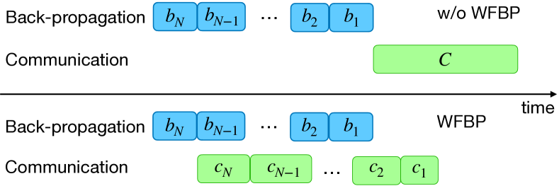
Figure 1: Distributed training without and with WFBP.

A DNN model consists of a number of layers. The distributed training involves three steps: 1) forward propagation, which takes as input a batch of training data, propagates it through the model, and calculates the loss function; 2) back-propagation, which computes the gradients of the parameters with the loss value layer by layer; 3) synchronization, which aggregates the gradient updates from all the workers and update the model.

Since back-propagation is performed layer by layer, the gradients of layer $l$ could be communicated during the computation of the gradients in layer $l-1$, as shown in Figure 1. In other words, the communication begins before the completion of the computation. This wait-free back-propagation (WFBP) mechanism significantly reduces the communication overhead by overlapping the communication with the computation (Zhang et al., 2017; Sergeev & Del Balso, 2018; Li et al., 2020; Peng et al., 2019).

Because of WFBP, existing distributed ML frameworks, such as PyTorch (Paszke et al., 2019), TensorFlow (Abadi et al., 2016), and Horovod (Sergeev & Del Balso, 2018), apply compression algorithms layer by layer for distributed training to further reduce the communication time. In addition, it is explicitly mentioned in many papers that the compression algorithms are applied in a layer-wise fashion (Karimireddy et al., 2019; Lim et al., 2018; Wen et al., 2017; Chen et al., 2018; Aji & Heafield, 2017).

3 The Practical Performance of Compression Algorithms

In this section, we first measure the practical performance of popular compression algorithms for distributed training. We then analyze the root cause of their poor performance and discuss the challenge to address it.

3.1 Performance measurement

To profile the performance of gradient compression, we empirically measure the training speed of popular compression algorithms, including both sparsification and quantization. Suppose the training speed with $n$ workers is $T_{n}$. The scaling factor (Zhang et al., 2020) is defined as

$$\small\textup{scaling factor}=\frac{T_{n}}{nT_{1}}.$$

Setup. All experiments are conducted on a server equipped with 8 GPUs (NVIDIA Tesla V100 with 32 GB memory), two 20-core/40-thread processors (Intel Xeon Gold 6230 2.1GHz), PCIe 3.0 $\times$16, and NVLink. The server has an Ubuntu 18.04.4 LTS system and the software environment includes PyTorch-1.7.1, Horovod-0.21.1, CUDA-10.1, Open MPI-4.0.2 and NCCL-2.8.3. The batch size is 64 and the gradient sparsity of sparsification algorithms is 99%.

The evaluated schemes and their corresponding communication primitives  are shown in Table 1. Allreduce is used for FP32 and FP16 (Sergeev & Del Balso, 2018; Li et al., 2020; NCC, 2021); allgather is used for other schemes because allreduce does not support sparse tensors and requires input tensors to be of the same data type and dimension for reduction (Xu et al., 2020; Renggli et al., 2019).

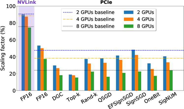
Figure 2: The scaling factors of ResNet50 on CIFAR10 with various compression algorithms, which apply layer-wise compression. It shows that compression algorithms do not scale well.

(a) Encoding overhead

(b) Decoding overhead

(c) Number of tensors across different sizes

Figure 3: The computation overhead of each tensor with different compression algorithms. An element is an FP32 gradient. Both encoding and decoding overheads are non-negligible. The total number of tensors for synchronization in ResNet50 and ResNet101 is 161 and 314.

Commnuicator	Allreduce	Allgather
Schemes	FP32	DGC, Top-k, Rand-k, EFSignSGD
	FP16	QSGD, SignSGD, OneBit, SigNUM
Library	MPI/PCIe	MPI/PCIe
	NCCL2/NVLink

Table 1: The evaluated schemes and their communication settings.

Figure 2 shows the scaling factors of different compression algorithms with layer-wise compression for ResNet50 on CIFAR10 . The baselines for both NVLink and PCIe are the performance of FP32. We observe that these compression algorithms do not scale well. Moreover, the performance of most compression algorithms is surprisingly worse than the baseline. Some algorithms, such as Top-k (Aji & Heafield, 2017), DGC (Lin et al., 2017) and OneBit (Seide et al., 2014), decrease the performance by more than 30% compared to the baseline on PCIe.

3.2 The root cause of the poor performance

There are two additional operations for gradient compression algorithms compared with vanilla distributed training: encoding (compress the gradients for communication) and decoding (decompress the received compressed gradients for model update). Figure 3(a) and 3(b) display the encoding and decoding overhead of each tensor with different compression algorithms. Both encoding and decoding overheads are non-negligible, even for small tensor sizes. For instance, the encoding overhead of most compression algorithms is greater than 0.1 ms and the decoding overhead is greater than 0.03 ms, regardless of the tensor sizes. Furthermore, many compression algorithms leverage error-feedback (Seide et al., 2014; Strom, 2015; Wu et al., 2018; Stich et al., 2018; Lin et al., 2017) to preserve the accuracy, incurring another decoding operation.

DNN models tend to have a large number of tensors for gradient synchronization. For instance, there are 161 tensors in ResNet50 and 314 tensors in ResNet101, as shown in Figure 3(c). Layer-wise compression invokes encoding-decoding operations for each tensor and the costly compression overhead dramatically suppresses the communication improvement.

We take training ResNet50 on CIFAR10 with 2GPUs connected by PCIe as a concrete example to compare the overall compression overhead against the communication improvement. In our measurement, the iteration time of single-GPU training is around 64 ms. Without any compression, the communication overhead  in each iteration is about 66 ms. Sparsification and 1-bit quantization algorithms can reduce the communication overhead to less than 5 ms thanks to the much smaller communicated data size. However, performing gradient compression to reduce communicated data size is not free. For instance, the overall estimated compression overheads of EFSignSGD (Karimireddy et al., 2019) and DGC (Lin et al., 2017) are around 65 ms and 120 ms, which are close to or even higher than the communication overhead without compression. The compression overhead leads to the poor practical performance of compression algorithms and becomes their performance bottleneck.

3.3 An opportunity and a challenge

The layer-wise compression overhead of compression algorithms is non-negligible. There are some fixed overheads to launch and execute kernels in CUDA (Arafa et al., 2019) and we observe that the encoding and decoding overheads remain quite stable across a wide range of tensor sizes. For many algorithms, the compression overhead increases by less than 50% from the tensor size of $2^{6}$ to $2^{20}$ elements. This observation indicates that merging multiple tensors for one encoding-decoding operation can potentially reduce the overall compression overhead.

However, merging tensors for compression algorithms raises a new challenge: how to merge tensors to achieve the optimal performance? There is a trade-off between the compression overhead and the communication overhead because merging tensors to reduce the compression overhead is at the cost of the overlap between the computation and communication. For example, an extreme case of merging tensors is to apply compression algorithms to the entire model with only one encoding-decoding operation. However, the communication cannot begin until the computation completes, resulting in the suboptimal communication overhead, as shown in Figure 1.

The optimal merging strategy depends on the compression algorithms, the DNN models and the system parameters, such as the number of workers, the network bandwidth, etc. We propose MergeComp to address the challenge to realize the promised benefits of gradient compression algorithms.

4 MergeComp

In this section, we will first introduce MergeComp to optimize the performance of gradient compression algorithms. We then demonstrate that MergeComp preserves the convergence rate of the applied compression algorithms. We next describe how MergeComp automatically determines efficient merging strategies for distributed training. The selected merging strategy is equivalent to a schedule for applying compression operations during training.

4.1 Overview

MergeComp aims to reduce the operation overhead for compression algorithms and meanwhile overlap the computation and communication to reduce the communication overhead.

Algorithm 1 describes how MergeComp works to optimize the performance of compression algorithms. A model is partitioned into $y$ groups, i.e., $\mathcal{X}=\{\rm x_{1},\dots,\rm x_{y}\}$, and $\rm x_{i,t}$ is $\rm x_{i}$ in the $t_{th}$ iteration. Tensors that belong to the same group are merged and compressed together in one compression operation. $K$ is the total number of iterations for the training. The compression algorithm $\mathcal{C}(\cdot)$ could be either sparsification or quantization. MergeComp performs an encoding-decoding operation and communication on each group in each iteration. After compression, a set of communication schemes, such as allreduce (Patarasuk & Yuan, 2009; Sergeev & Del Balso, 2018), allgather (Thakur et al., 2005) or parameter servers (Li et al., 2014), could be used for the synchronization of different compression algorithms. The communication is overlapped with back-propagation to reduce the communication overhead. After communication, the compressed gradients are decompressed and aggregated to update the model.

Algorithm 1 MergeComp for compression algorithms. The communication is overlapped with computation.

  Input: model $\rm\mathcal{X}=\{\rm x_{1},\dots,\rm x_{y}\}$, learning rate $\gamma$, and compression algorithm $\mathcal{C}(\cdot)$

  for $t=0$ to $K-1$ do

    for $i=1$ to $y$ do

       ${\rm g}_{i,t}\coloneqq$ stochasticGradient(${\rm x}_{i,t}$)

       ${\rm\delta}_{i,t}\coloneqq\mathcal{C}({\rm g}_{i,t})$

       $\Delta_{i,t}\coloneqq$ communicate(${\rm\delta}_{i,t}$)

       $\tilde{\rm g}_{i,t}\coloneqq$ aggregate($\mathcal{C}^{-1}(\Delta_{i,t})$)

       ${\rm x}_{i,t+1}$ = ${\rm x}_{i,t}-\gamma\tilde{\rm g}_{i,t}$

    end for

  end for

4.2 MergeComp guarantees

We will analyze the convergence rate of distributed training with sparse or quantized communication scheduled by MergeComp. The analysis in this paper focuses on synchronous data-parallel distributed SGD.

4.2.1 Notation and assumptions

Let $F(\cdot)$ be the loss function we want to optimize and the studied stochastic optimization problem is

$$\small\min f(x)\coloneqq\frac{1}{n}\sum\limits_{i=1}^{n}\underbrace{\mathbb{E}_{\xi\sim\mathcal{D}_{i}}F_{i}(x;\xi)}_{\text{$=:f_{i}(x)$}},$$ (1)

where $n$ is the number of workers for the training, $\mathcal{D}_{i}$ is a predefined distribution for the training data on worker $i$ and $F_{i}(x;\xi)$ is the loss computed from samples on worker $i$.

Notation. In the analysis of this subsection, $\left\|\cdot\right\|_{2}$ denotes the L2 norm of a vector or the spectral norm of a matrix; $\nabla f(\cdot)$ denotes the gradient of a function $f$; $\textbf{1}_{n}$ denotes the column vector in $\mathbb{R}^{n}$ with 1 for all elements; $f^{*}$ denotes the optimal solution for the stochastic optimization problem.

We employ standard assumptions of the loss function and the variance of the stochastic gradient for the analysis.

Assumption 1.

(Lipschiz continuity) $\nabla f(\cdot)^{{}^{\prime}}$ is Lipschitz continuous with respect to the L2 norm, i.e.,

$$\small\left\|\nabla f_{i}(x)-\nabla f_{i}(y)\right\|_{2}\leq L\left\|x-y\right\|_{2}\qquad\forall x,\forall y,\forall i.$$ (2)

Assumption 2.

(Bounded variance) The variance of stochastic gradient is bounded, i.e.,

$$\small\mathbb{E}_{\xi\sim\mathcal{D}_{i}}\left\|\nabla F_{i}(x;\xi)-\nabla f_{i}(x)\right\|_{2}^{2}\leq\sigma^{2}\qquad\forall x,\forall i.$$ (3)

Assumption 3.

(Unbiasness) The stochastic gradient of $F_{i}(x;\xi)$ is unbiased, i.e.,

$$\small\mathbb{E}_{\xi\sim\mathcal{D}_{i}}\nabla F_{i}(x;\xi)=\nabla f_{i}(x)\qquad\forall x,\forall i.$$ (4)

Assumption 4.

Sparsification algorithms can exchange all the gradients in any $p$ consecutive iterations.

These assumptions are commonly employed in previous works to analyze the convergence rate of distributed SGD (Jiang & Agrawal, 2018; Alistarh et al., 2017; Ghadimi & Lan, 2013; Wen et al., 2017; Lian et al., 2017).

4.2.2 Sparse communication

Previous works proved that a subset of gradients can achieve the same convergence rate as vanilla distributed SGD (Stich et al., 2018; Jiang & Agrawal, 2018; Basu et al., 2019). Since MergeComp still selects important gradients in each group for sparse communication, it preserves the convergence rate as the applied sparsification algorithms.

Under Assumptions 1-4, we have the following theorem for any sparsification algorithms with MergeComp.

Theorem 1.

If all workers share the same training dataset, setting $\gamma=\theta\sqrt{M/K}$ where $\theta>0$ is a constant, $M$ is the total mini-batch size on all workers, $L\gamma\leq 1$ and $6np^{2}L^{2}\gamma^{2}<1$, MergeComp for sparsification algorithms has the convergence rate as

$$\begin{split}\small&\frac{1}{K}(\sum\limits_{t=0}^{K-1}\left\|\nabla f(\frac{X_{t}1_{n}}{n})\right\|_{2}^{2})\\ \leq&\frac{4\theta^{-1}(f(x_{0})-f^{\textstyle*})+2\theta L\sigma^{2}}{\sqrt{MK}}+\frac{2pn^{2}\theta^{2}L^{2}\sigma^{2}}{K},\end{split}$$ (5)

if the number of iterations satisfies $K\geq 12nM\theta^{2}p^{2}L^{2}$.

Theorem 1 has a similar structure and proof to Corollary 1 in (Jiang & Agrawal, 2018), while with different assumption of the training dataset. In Theorem 1, $\frac{X_{j}1_{n}}{n}$ is the average of the gradients on all workers. If $K$ is large enough, the right side in (5) is dominated by its first term and MergeComp for sparsification algorithms can converge at rate $\mathcal{O}(1/\sqrt{MK})$, the same rate as vanilla SGD (Stich et al., 2018). See the supplemental materials for the proof to Theorem 1.

4.2.3 Quantized communication

Let $\mathcal{Q}(\cdot)$ denote the quantization compressor. The bound of expected error of $\mathcal{Q}(\cdot)$ is defined as $q_{i}=\sup\frac{\left\|\mathcal{Q}(\rm x_{i})-\rm x_{i}\right\|_{2}^{2}}{\left\|\rm x_{i}\right\|_{2}^{2}}$, where $\rm x_{i}$ is the gradients in the $i_{th}$ group. We also define $q=\max\{q_{i}\}$ to derive the convergence rate of quantization algorithms with MergeComp under Assumption 1-3.

Theorem 2.

If all workers share the same training dataset and error feedback is applied, setting $\gamma=\theta\sqrt{M/K}$ where $\theta>0$ is a constant and $(1+\frac{q}{n})L\gamma<2$, MergeComp for quantization algorithms has the following convergence rate:

$$\begin{split}\small&\frac{1}{K}(\sum\limits_{t=0}^{K-1}\left\|\nabla f(x_{t})\right\|_{2}^{2})\\ \leq&\frac{2\theta^{-1}(f(x_{0})-f^{\textstyle*})+(1+q)\theta L\sigma^{2}y}{\sqrt{MK}},\end{split}$$ (6)

if the number of iterations satisfies $K\geq M\theta^{2}L^{2}(1+\frac{q}{n})^{2}$.

Theorem 2 shows that MergeComp for quantization algorithms can also converge at rate $\mathcal{O}(1/\sqrt{MK})$. See the supplemental materials for the proof to Theorem 2.

4.3 Searching for the optimal model partition

We will explore how to determine the optimal partitioning strategy for distributed training. We formulate the model partition problem as an optimization problem.

Notation. Let $N$ denote the number of tensors of a model and $A$ the computation time of each iteration. Let $y$ be the number of partitioned groups, $x_{i}$ the size of the $i_{th}$ group (i.e., $x_{i}=|\rm x_{i}|$), and $X_{y}=\{x_{1},\dots,x_{y}\}$ a partition of the model. Recall that tensors belonging to the same group are merged for compression. $h(x_{i})$ is the compression time of the $i_{th}$ group, $g(x_{i})$ is its communication time, and $p(x_{i})$ is the overlap time between the computation and communication time.

The goal of searching for the optimal partition is to minimize the iteration time for compression algorithms. Without WFBP, the iteration time is the summation of the computation time, the compression time, and the communication time; while with WFBP, the overlap time helps reduce the communication overhead. Therefore, the optimization objective of the model partition problem is to

$$\small\min\limits_{y\in[1,N]}\min\limits_{X_{y}\in\mathcal{X}_{y}}F(X_{y})\coloneqq A+\sum\limits_{i=1}^{y}h(x_{i})+\sum\limits_{i=1}^{y}g(x_{i})-\sum\limits_{i=1}^{y}p(x_{i}),$$ (7)

where $\mathcal{X}_{y}$ is the set of all possible partitions with $y$ groups.

Lemma 1.

The size of the search space for the model partition problem is $2^{N-1}$.

Lemma 1 indicates that the general form of the model partition problem cannot be solved in polynomial time. In practice, the compression time and the communication time both increases with the group size. Therefore, we make the following assumption for the model partition problem.

Assumption 5.

(Linear overhead) $h(x_{i})=B_{h}+\gamma_{h}x_{i}$ and $g(x_{i})=B_{g}+\gamma_{g}x_{i}$, where $B_{h}$ and $B_{g}$ are the latency (or startup time) for the compression and communication time; $\gamma_{h}$ and $\gamma_{g}$ are the overheads for each unit.

Under Assumption 5, we have the following lemma.

Lemma 2.

Given a particular $y$, all possible partitions have the same compression time and communication time; and they both increase with the value of $y$.

Algorithm 2 A heuristic algorithm for model partition

  Input: $Y\in[2,N]$, $\alpha\in(0,1)$

  $F_{min}(1)=F(X_{1})$

  for $y=2$ to $Y$ do

    $X_{y}^{\textstyle*}=\operatorname*{arg\,min}\limits_{X_{y}\in\mathcal{X}_{y}}F(X_{y})$

    $F_{min}(y)=F(X_{y}^{\textstyle*})$

    if $F_{min}(y-1)<F_{min}(y)$ then

       return $X_{y-1}^{\textstyle*}$

    else if $F_{min}(y-1)-F_{min}(y)<\alpha F_{min}(y-1)$ then

       return $X_{y}^{\textstyle*}$

    end if

  end for

  return $X_{y}^{\textstyle*}$

There are two empirical observations for the model partition problem: 1) increasing the number of partition groups helps increase the overlap time, but it also increases the overhead of compression and communication time according to Lemma 2; and 2) the marginal benefit of the overlap time is diminishing with the increasing number of groups. Based on these two observations, we propose a heuristic algorithm to approximately solve the model partition problem in polynomial time, as shown in Algorithm 2.

MergeComp searches for an efficient model partition with Algorithm 2 at the beginning of training. $Y$ and $\alpha$ are two parameters to narrow down the search space. For any $y\in[2,Y]$, the algorithm searches for the optimal partition $X_{y}^{\textstyle*}$ (refer to the proof to Theorem 3 for the details) and then compares the iteration time with $X_{y-1}^{\textstyle*}$. If its performance is worse than $X_{y-1}^{\textstyle*}$ or the marginal benefit is less than $\alpha F_{min}(y-1)$, the algorithm terminates the search and the best partition strategy discovered by Algorithm 2 is used for the remaining training iterations.

Theorem 3.

The time complexity of Algorithm 2 to solve the model partition problem is $O(N^{Y-2}\log N)$.

See the supplemental materials for the proof to Theorem 3. We experimentally observe that Algorithm 2 works very well in practice to achieve good scalability for distributed training. Furthermore, it makes no assumption of model architectures or system parameters (e.g., the batch size, the number of GPUs, and network bandwidth capacities) to search for an efficient model partition.

5 Experiments

In this section, we will first show the performance improvement of MergeComp for various compression algorithms over both PCIe and NVLink. We then use end-to-end experiments to demonstrate that MergeComp can preserve the accuracy of the applied compression algorithms.

(a) 2 GPUs

(b) 4 GPUs

(c) 8 GPUs

Figure 4: The performance of ResNet50 on CIFAR10. The scaling factor of MergeComp is up to 2.91$\times$ and 3.83$\times$ (DGC with 8 GPUs) higher than that of the baseline and layer-wise compression.

(a) 2 GPUs

(b) 4 GPUs

(c) 8 GPUs

Figure 5: The performance of ResNet101 on ImageNet. The scaling factor of MergeComp is up to 1.68$\times$ and 2.46$\times$ (DGC with 8 GPUs) higher than that of the baseline and layer-wise compression. Legend in Figure 4.

(a) 2 GPUs

(b) 4 GPUs

(c) 8 GPUs

Figure 6: The performance of Mask R-CNN on COCO. The scaling factor of MergeComp is up to 2.33$\times$ and 1.66$\times$ (DGC with 8 GPUs) higher than that of the baseline and layer-wise compression. Legend in Figure 4.

Setup. The setup is the same as that described in Section 3.

Workloads. We validate the performance of MergeComp on two types of machine learning tasks: image classification and image segmentation. The models include ResNet50 and ResNet101 (He et al., 2016) on CIFAR10 (Krizhevsky et al., 2009) and ImageNet (Deng et al., 2009); Mask R-CNN (He et al., 2017) on COCO (Lin et al., 2014). These three models are widely used as standard benchmarks to evaluation the scalability of distributed training. The default batch size for image classification is 64 and image segmentation is 1.

Methods. We benchmark the tasks with MergeComp and set $Y=2,3,4$ for the evaluation. We compare them against FP32 (baseline) and layer-wise compression. The gradient sparsity of sparsification algorithms is 99% and each FP32 element is mapped to 8 bits in QSGD (Alistarh et al., 2017).

Metrics. We use the scaling factor and Top-1 accuracy as evaluation metrics. The results for scaling factors are reported with the average of 20 runs. We also report the standard deviation using the error bar because the training speed varies at times.

5.1 Training speed improvement

We apply MergeComp to nine popular compression algorithms for three DNN models. Figures 4-6 present the performance of various compression algorithms with $Y=2$. We omit the results of MergeComp with $Y=3$ and $Y=4$ since they have very similar performance to that with $Y=2$. We evaluate the choice of $Y$ in Section 5.2.

MergeComp can significantly improve the performance of both sparsification and quantization algorithms. For instance, on PCIe, the scaling factor of MergeComp with DGC for ResNet50 on CIFAR10 is up to 2.91$\times$ and 3.83$\times$ higher than that of the baseline and layer-wise compression. Similarly, MergeComp improves the scaling factor of ResNet101 on ImageNet by 1.68$\times$ and 2.46$\times$ compared to the baseline and layer-wise compression. There is no obvious improvement for Top-k because its performance bottleneck is still the compression overhead, i.e., the time-consuming top-k() operation.

MergeComp can help distributed training achieve near-linear scalability on NVLink. With FP32, the scaling factor of ResNet50 on CIFAR10 with 8 GPUs is about 75%. Converting the gradients from FP32 to FP16 for communication decreases the performance because of the compression overhead, but applying MergeComp to FP16 improves the scaling factors to 92%. Similarly, MergeComp achieves the scaling factors of 99% and 96% for ResNet101 on ImageNet with 4 GPUs and 8 GPUs, respectively.

For 1 bit quantization algorithms, e.g., EFSignSGD (Karimireddy et al., 2019), SignSGD (Bernstein et al., 2018a), OneBit (Seide et al., 2014) and SigNUM (Bernstein et al., 2018b), the scaling factor of MergeComp for ResNet50 is up to 2.60$\times$ and 3.18$\times$ higher than that of the baseline and layer-wise compression. The corresponding improvements for ResNet101 are 1.56$\times$ and 2.24$\times$, respectively.

Layer-wise compression for Mask R-CNN has better performance than the baseline over PCIe because it has relatively few tensors so the layer-wise compression overhead is not too excessive. MergeComp still outperforms layer-wise compression by up to 1.66$\times$ on PCIe and 1.1$\times$ on NVLink.

5.2 The model partition algorithm

We evaluate the effectiveness of the proposed heuristic algorithm, which searches for the near-optimal partitioning strategy for distributed training. The evaluated model is ResNet101 on ImageNet. MergeComp is applied to three representative compression algorithms: FP16, DGC and EFSignSGD.

Table 2 shows the performance of MergeComp with different values of $Y$. The results are normalized against the performance of MergeComp with $Y=1$. It shows that partitioning the model into more than one groups could improve the scalability and the achieved improvement of MergeComp increases with the number of GPUs. It is because the communication overhead increases with the number of GPUs and MergeComp can search for the near-optimal partition to optimize the communication overhead.

The performance of MergeComp with $Y=3$ and $Y=4$ is very close to that with $Y=2$ . The observation is that it is a good choice to set $Y=2$ for MergeComp because the marginal benefit of a larger $Y$ is negligible. Moreover, because the time complexity of Algorithm 2 is $O(N^{Y-2}\log N)$, a larger $Y$ requires many more iterations to search for an efficient model partition than $Y=2$, which needs less than 50 iterations in our evaluation.

We also compare the performance of MergeComp with a naive partition strategy, which evenly partitions the number of tensors to each group. As shown in Table 3, the performance of MergeComp is up to 5.5% higher than that of the naive partition with $Y=2$.

Compressor	$Y=2$			$Y=3$
	2GPUs	4GPUs	8GPUs	2GPUs	4GPUs	8GPUs
FP16	1.16$\times$	1.18$\times$	1.23$\times$	1.16$\times$	1.18$\times$	1.23$\times$
DGC	1.04$\times$	1.06$\times$	1.06$\times$	1.04$\times$	1.06$\times$	1.06$\times$
EFSignSGD	1.04$\times$	1.05$\times$	1.13$\times$	1.04$\times$	1.04$\times$	1.13$\times$

Table 2: The performance of MergeComp with different number of partition groups $Y$. The numbers are normalized against the performance of MergeComp with $Y=1$.

Compressor	2 GPUs	4 GPUs	8 GPUs
FP16	5.5%	5.4%	5.1%
DGC	2.0%	1.9%	1.9%
EFSignSGD	3.4%	3.3%	3.1%

Table 3: The performance improvement of MergeComp compared against the naive partition with $Y=2$.

5.3 End-to-end experiments

Figure 7: The performance of MergeComp for ResNet50 on CIFAR10. The applied compression algorithm is DGC. The time required for convergence with MergeComp is 2.27$\times$ and 3.28$\times$ lower than that of the baseline and layer-wise compression.

Figure 8: The performance of MergeComp for ResNet50 on ImageNet. The applied compression algorithm is EFSignSGD.

We apply MergeComp to EFSignSGD and DGC to show its performance for end-to-end training with 4 GPUs connected by PCIe. Figure 7 illustrates the time and iteration wise comparisons of ResNet50 on CIFAR10. The time required for convergence with MergeComp is 2.27$\times$ and 3.28$\times$ lower than that of the baseline and layer-wise compression.

Similarly, Figure 8 illustrates the performance comparison for ResNet50 on ImageNet. The time required for convergence with MergeComp is 1.28$\times$ and 1.42$\times$ lower than that of the baseline and layer-wise compression; and the scaling factor of MergeComp achieves around 90%.

Compressor	Datasets	Methods	Top-1 Accuracy
DGC	CIFAR10	Baseline	93.6%
		Layer wise	93.5%
		MergeComp	93.5%
EFSignSGD	ImageNet	Baseline	75.4%
		Layer wise	75.2%
		MergeComp	75.2%

Table 4: Top-1 validation accuracy of ResNet50.

Table 4 shows the Top-1 validation accuracy of ResNet50 on both CIFAR10 and ImageNet with different methods. Compared with layer-wise compression, MergeComp can preserve the accuracy of the applied compression algorithms.

6 Related Work

There are two directions to improve communication efficiency of large-scale distributed training: 1) higher network bandwidth capacity and 2) smaller communicated data size. High-bandwidth network devices are equipped to accelerate distributed training. For instance, NVLink and NVSwitch (NVL, 2020) are widely used for intra-machine GPU-to-GPU interconnection and RDMA (Xue et al., 2019; Jiang et al., 2020) for intra-rack communication. Unfortunately, even with these advanced hardware, the performance of large-scale distributed training is still far from near-linear scalability because of the large model sizes (Wang et al., 2019; Zhang et al., 2020). Besides sparsification and quantization algorithms, low-rank compression algorithms (Vogels et al., 2019; Cho et al., 2019; Idelbayev & Carreira-Perpinán, 2020) are also proposed to reduce the communicated data size. Local SGD (Stich, 2018; Woodworth et al., 2020; Lin et al., 2018) allows the model to evolve locally on each machine for multiple iterations and then synchronize the gradients. It can help compression algorithms further reduce the communication overhead. Distributed ML frameworks batch multiple tensors for one communication operation to improve the communication performance (Sergeev & Del Balso, 2018; Li et al., 2020; Chen et al., 2015; Jiang et al., 2020), but this mechanism happens after compression and is orthogonal to gradient compression algorithms.

7 Conclusion

We propose MergeComp, a compression scheduler to optimize the scalability of distributed training. It automatically schedules the compression operations to optimize the performance of compression algorithms without the knowledge of model architectures or system parameters. Extensive experiments demonstrate that MergeComp can significantly improve the performance of distributed training over state-of-the-art communication methods without losing accuracy.

8 Acknowledgement

We would like to thank the BOLD Lab members for their useful feedback. This research is sponsored by the NSF under CNS-1718980, CNS-1801884, and CNS-1815525.

9 Supplemental Materials

Assumption 6.

The variance of gradient among workers is bounded, that is

$$\small\mathbb{E}_{i\sim\mathcal{U}(1,n)}\left\|\nabla f_{i}(x)-\nabla f(x)\right\|_{2}^{2}\leq\zeta^{2}\qquad\forall x,$$

where $\mathcal{U}(1,n)$ is a discrete uniform distribution of integers from 1 to $n$. If all workers share the same training data, $\zeta=0$.

9.1 Proof to Theorem 1

Proof.

Refer to a corollary in (Jiang & Agrawal, 2018) and we restate it here:

Corollary 1.

(Jiang & Agrawal, 2018) Under Assumptions 1-4 and 6, if setting $\gamma=\theta\sqrt{M/K}$ where $\theta>0$ is a constant, we have the convergence rate for sparsification algorithms as:

$$\small\frac{1}{K}(\sum\limits_{t=0}^{K-1}\left\|\nabla f(\frac{X_{t}1_{n}}{n})\right\|_{2}^{2})\\ \leq\frac{4\theta^{-1}(f(x_{0})-f*)+2\theta L\sigma^{2}}{\sqrt{MK}}+\frac{2pn^{2}\theta^{2}L^{2}\sigma^{2}+6nM\theta^{2}p^{2}L^{2}\zeta^{2}}{K},$$ (8)

if the number of iterations satisfies $K\geq 12nM\theta^{2}p^{2}L^{2}$.

Since we assume all workers share the same training dataset, we can remove the items with $\zeta$ in Inequality (8) and have Theorem 1.

∎

9.2 Proof to Theorem 2

Proof.

The proof is based on a corollary in (Jiang & Agrawal, 2018) and we restate it here:

Corollary 2.

(Jiang & Agrawal, 2018) Under Assumptions 1-4 and 6, if using a quantization function with an error bound of $q$ and and setting $\gamma=\theta\sqrt{M/K}$ where $\theta>0$ is a constant, we have the following convergence rate for quantization algorithms:

$$\small\frac{1}{K}(\sum\limits_{t=0}^{K-1}\left\|\nabla f(x_{t})\right\|_{2}^{2})\leq\frac{2\theta^{-1}(f(x_{0})-f^{\textstyle*})+(1+q)\theta L\sigma^{2}}{\sqrt{MK}}+\frac{m}{\sqrt{MK}}\theta qL\zeta^{2},$$ (9)

if the number of iterations satisfies $K\geq M\theta^{2}L^{2}(1+\frac{q}{n})^{2}$.

Since we assume all workers share the same training dataset, we can remove the items with $\zeta$ in Inequality (9) and have the following inequality

$$\small\begin{split}\frac{1}{K}(\sum\limits_{t=0}^{K-1}\left\|\nabla f({\rm x}_{i,t})\right\|_{2}^{2})&\leq\frac{2\theta^{-1}(f({\rm x}_{i,0})-f^{\textstyle*}({\rm x}_{i}))+(1+q_{i})\theta L\sigma^{2}}{\sqrt{MK}}\\ &\leq\frac{2\theta^{-1}(f({\rm x}_{i,0})-f^{\textstyle*}({\rm x}_{i}))+(1+q)\theta L\sigma^{2}}{\sqrt{MK}},\end{split}$$ (10)

where $\rm x_{i,t}$ is $x_{i}$ at the $t_{th}$ iteration and $q=\max\{q_{i}\}$. Since $\left\|\nabla f({\rm x})\right\|_{2}^{2}=\sum\limits_{i=1}^{y}\left\|\nabla f({\rm x}_{i})\right\|_{2}^{2}$, we have

$$\small\begin{split}\frac{1}{K}(\sum\limits_{t=0}^{K-1}\left\|\nabla f(x_{t})\right\|_{2}^{2})&=\sum\limits_{i=1}^{y}\frac{1}{K}(\sum\limits_{t=0}^{K-1}\left\|\nabla f({\rm x}_{i,t})\right\|_{2}^{2})\\ &\leq\frac{2\theta^{-1}(\sum\limits_{i=1}^{y}f({\rm x}_{i,0})-\sum\limits_{i=1}^{y}f^{\textstyle*}({\rm x}_{i}))+(1+q)\theta L\sigma^{2}y}{\sqrt{MK}}\\ &\leq\frac{2\theta^{-1}(f(x_{0})-\sum\limits_{i=1}^{y}f^{\textstyle*}({\rm x}_{i}))+(1+q)\theta L\sigma^{2}y}{\sqrt{MK}}\\ \end{split}$$ (11)

Because $f^{\textstyle*}$ is the optimal solution, we have $f^{\textstyle*}\leq\sum\limits_{i=1}^{y}f^{\textstyle*}({\rm x}_{i})$ and Inequality (12) can be rewritten as

$$\small\begin{split}\frac{1}{K}(\sum\limits_{t=0}^{K-1}\left\|\nabla f(x_{t})\right\|_{2}^{2})\leq\frac{2\theta^{-1}(f(x_{0})-f^{\textstyle*})+(1+q)\theta L\sigma^{2}y}{\sqrt{MK}}\end{split}$$ (12)

∎

9.3 Proof to Theorem 3

9.3.1 Proof to Lemma 1

Proof.

Given a particular $y$, the number of possible partitions with $y$ groups is $\binom{N-1}{y-1}$. Since $y\in[1,N]$, the total number of possible partitions is $\sum_{y=1}^{N}\binom{N-1}{y-1}=2^{N-1}$. ∎

9.3.2 Proof to Lemma 2

Proof.

Given a partition $X_{y}=\{x_{1},\dots,x_{y}\}$, the overall compression time is $\sum_{i=1}^{y}h(x_{i})=yB_{h}+\gamma_{h}D$ and the overall communication time is $\sum_{i=1}^{y}g(x_{i})=yB_{g}+\gamma_{g}D$, where $D$ is the model size. These two expressions are both monotonically increasing functions of $y$. ∎

9.3.3 Proof to Theorem 3

Proof.

We first prove that $X_{2}^{\textstyle*}$ can be solved in $O(\log N)$. Suppose $X_{2}=\{x_{1},x_{2}\}=\{x_{1},D-x_{1}\}$, where $D$ is the model size. There are two cases for the overlap time of the first partition group: its communication time is completely or partly overlapped with the computation of the second group. With a small $x_{1}$, $g(x_{1})$ is completely overlapped and $p(x_{1})$ increases with $x_{1}$. At a turning point ($x_{1}^{\textstyle*}$), the communication of the first group cannot be finished before the computation of the second group completes so that it comes to the second case. In this case, the communication of the second group can begin right after the communication of the first one and $p(x_{1})$ is the computation time of the second group so that $p(x_{1})$ decreases with $x_{1}$. According to Lemma 2, both the compression and communication time is constant. Therefore, $F(X_{2})$ decreases in $(0,x_{1}^{\textstyle*}]$ and increases in $(x_{1}^{\textstyle*},D)$. Searching for $X_{2}^{\textstyle*}$ (i.e., $x_{1}^{\textstyle*}$) can be solved with binary search in $O(\log N)$.

When $y>2$ and suppose $X_{y}=\{x_{1},\dots,x_{y}\}$, we can first fix $x_{1},\dots,x_{y-2}$ and then solve the optimal $x_{y-1}$ to minimize $F(X_{y})$. There are three cases for the communication of $x_{y-2}$: 1) $g(x_{y-2})$ is not overlapped; 2) $g(x_{y-2})$ is partly overlapped and 3) $g(x_{y-2})$ is completely overlapped. For cases 1) and 2), the value of $x_{y-1}$ will not affect $F(X_{y})$ because there is no overlap time for $x_{y-1}$ and $x_{y}$; for case 3), the optimal $x_{y-1}$ can be solved in $O(\log N)$ based on the above analysis. Since $\binom{N-2}{y-2}\log N<N^{y-2}\log N$, $X_{y}^{\textstyle*}$ can be solved in $O(N^{y-2}\log N)$. Therefore, Algorithm 2 can solve all optimal partition $X_{i}^{\textstyle*}$, where $2\leq i\leq Y$, in $O(N^{y-2}\log N)$ and return the best $X_{i}^{\textstyle*}$. ∎

References

- NVL (2020) NVLink and NVSwitch specification. https://www.nvidia.com/en-us/data-center/nvlink/, 2020.
- MLP (2021) MLPerf Training v0.7 Results. https://mlperf.org/training-results-0-7, 2021.
- NCC (2021) NVIDIA NCCL. https://developer.nvidia.com/NCCL, 2021.
- Abadi et al. (2016) Abadi, M., Barham, P., Chen, J., Chen, Z., Davis, A., Dean, J., Devin, M., Ghemawat, S., Irving, G., Isard, M., Kudlur, M., Levenberg, J., Monga, R., Moore, S., Murray, D. G., Steiner, B., Tucker, P., Vasudevan, V., Warden, P., Wicke, M., Yu, Y., and Zheng, X. Tensorflow: A system for large-scale machine learning. In USENIX Symposium on Operating Systems Design and Implementation (OSDI), pp. 265–283, 2016.
- Aji & Heafield (2017) Aji, A. F. and Heafield, K. Sparse communication for distributed gradient descent. 2017.
- Alistarh et al. (2017) Alistarh, D., Grubic, D., Li, J., Tomioka, R., and Vojnovic, M. QSGD: Communication-efficient SGD via gradient quantization and encoding. In Advances in Neural Information Processing Systems, pp. 1709–1720, 2017.
- Alistarh et al. (2018) Alistarh, D., Hoefler, T., Johansson, M., Konstantinov, N., Khirirat, S., and Renggli, C. The convergence of sparsified gradient methods. In Advances in Neural Information Processing Systems, 2018.
- Arafa et al. (2019) Arafa, Y., Badawy, A.-H. A., Chennupati, G., Santhi, N., and Eidenbenz, S. Low overhead instruction latency characterization for nvidia gpgpus. In 2019 IEEE High Performance Extreme Computing Conference (HPEC), pp. 1–8. IEEE, 2019.
- Basu et al. (2019) Basu, D., Data, D., Karakus, C., and Diggavi, S. Qsparse-local-SGD: Distributed SGD with quantization, sparsification and local computations. In Advances in Neural Information Processing Systems, pp. 14695–14706, 2019.
- Bernstein et al. (2018a) Bernstein, J., Wang, Y.-X., Azizzadenesheli, K., and Anandkumar, A. signSGD: Compressed optimisation for non-convex problems. arXiv preprint arXiv:1802.04434, 2018a.
- Bernstein et al. (2018b) Bernstein, J., Zhao, J., Azizzadenesheli, K., and Anandkumar, A. signsgd with majority vote is communication efficient and fault tolerant. arXiv preprint arXiv:1810.05291, 2018b.
- Chen et al. (2018) Chen, C.-Y., Choi, J., Brand, D., Agrawal, A., Zhang, W., and Gopalakrishnan, K. Adacomp: Adaptive residual gradient compression for data-parallel distributed training. In Thirty-Second AAAI Conference on Artificial Intelligence, 2018.
- Chen et al. (2015) Chen, T., Li, M., Li, Y., Lin, M., Wang, N., Wang, M., Xiao, T., Xu, B., Zhang, C., and Zhang, Z. Mxnet: A flexible and efficient machine learning library for heterogeneous distributed systems. arXiv preprint arXiv:1512.01274, 2015.
- Chilimbi et al. (2014) Chilimbi, T., Suzue, Y., Apacible, J., and Kalyanaraman, K. Project adam: Building an efficient and scalable deep learning training system. In 11th USENIX Symposium on Operating Systems Design and Implementation (OSDI), pp. 571–582, 2014.
- Cho et al. (2019) Cho, M., Muthusamy, V., Nemanich, B., and Puri, R. Gradzip: Gradient compression using alternating matrix factorization for large-scale deep learning, 2019.
- Deng et al. (2009) Deng, J., Dong, W., Socher, R., Li, L.-J., Li, K., and Fei-Fei, L. Imagenet: A large-scale hierarchical image database. In 2009 IEEE conference on computer vision and pattern recognition, pp. 248–255. Ieee, 2009.
- Dettmers (2015) Dettmers, T. 8-bit approximations for parallelism in deep learning. arXiv preprint arXiv:1511.04561, 2015.
- Ghadimi & Lan (2013) Ghadimi, S. and Lan, G. Stochastic first-and zeroth-order methods for nonconvex stochastic programming. SIAM Journal on Optimization, 23(4):2341–2368, 2013.
- Gupta et al. (2020) Gupta, V., Choudhary, D., Tang, P. T. P., Wei, X., Wang, X., Huang, Y., Kejariwal, A., Ramchandran, K., and Mahoney, M. W. Fast distributed training of deep neural networks: Dynamic communication thresholding for model and data parallelism, 2020.
- He et al. (2016) He, K., Zhang, X., Ren, S., and Sun, J. Deep residual learning for image recognition. In Proceedings of the IEEE conference on computer vision and pattern recognition, pp. 770–778, 2016.
- He et al. (2017) He, K., Gkioxari, G., Dollár, P., and Girshick, R. Mask r-cnn. In Proceedings of the IEEE international conference on computer vision, pp. 2961–2969, 2017.
- Idelbayev & Carreira-Perpinán (2020) Idelbayev, Y. and Carreira-Perpinán, M. A. Low-rank compression of neural nets: Learning the rank of each layer. In Proceedings of the IEEE/CVF Conference on Computer Vision and Pattern Recognition, pp. 8049–8059, 2020.
- Jiang & Agrawal (2018) Jiang, P. and Agrawal, G. A linear speedup analysis of distributed deep learning with sparse and quantized communication. In Advances in Neural Information Processing Systems, pp. 2525–2536, 2018.
- Jiang et al. (2020) Jiang, Y., Zhu, Y., Lan, C., Yi, B., Cui, Y., and Guo, C. A unified architecture for accelerating distributed DNN training in heterogeneous gpu/cpu clusters. In 14th USENIX Symposium on Operating Systems Design and Implementation (OSDI 20), pp. 463–479, 2020.
- Karimireddy et al. (2019) Karimireddy, S. P., Rebjock, Q., Stich, S. U., and Jaggi, M. Error feedback fixes signsgd and other gradient compression schemes. arXiv preprint arXiv:1901.09847, 2019.
- Krizhevsky et al. (2009) Krizhevsky, A., Hinton, G., et al. Learning multiple layers of features from tiny images. 2009.
- Li et al. (2014) Li, M., Andersen, D. G., Park, J. W., Smola, A. J., Ahmed, A., Josifovski, V., Long, J., Shekita, E. J., and Su, B.-Y. Scaling distributed machine learning with the parameter server. In USENIX Symposium on Operating Systems Design and Implementation (OSDI), 2014.
- Li et al. (2020) Li, S., Zhao, Y., Varma, R., Salpekar, O., Noordhuis, P., Li, T., Paszke, A., Smith, J., Vaughan, B., Damania, P., and Chintala, S. Pytorch distributed: Experiences on accelerating data parallel training. arXiv preprint arXiv:2006.15704, 2020.
- Li et al. (2018a) Li, Y., Park, J., Alian, M., Yuan, Y., Qu, Z., Pan, P., Wang, R., Schwing, A., Esmaeilzadeh, H., and Kim, N. S. A network-centric hardware/algorithm co-design to accelerate distributed training of deep neural networks. In 2018 51st Annual IEEE/ACM International Symposium on Microarchitecture (MICRO), pp. 175–188. IEEE, 2018a.
- Li et al. (2018b) Li, Y., Park, J., Alian, M., Yuan, Y., Qu, Z., Pan, P., Wang, R., Schwing, A., Esmaeilzadeh, H., and Kim, N. S. A network-centric hardware/algorithm co-design to accelerate distributed training of deep neural networks. In 2018 51st Annual IEEE/ACM International Symposium on Microarchitecture (MICRO), pp. 175–188. IEEE, 2018b.
- Lian et al. (2017) Lian, X., Zhang, C., Zhang, H., Hsieh, C.-J., Zhang, W., and Liu, J. Can decentralized algorithms outperform centralized algorithms? a case study for decentralized parallel stochastic gradient descent. In Advances in Neural Information Processing Systems, pp. 5330–5340, 2017.
- Lim et al. (2018) Lim, H., Andersen, D. G., and Kaminsky, M. 3LC: Lightweight and effective traffic compression for distributed machine learning. arXiv preprint arXiv:1802.07389, 2018.
- Lin et al. (2018) Lin, T., Stich, S. U., Patel, K. K., and Jaggi, M. Don’t use large mini-batches, use local sgd. arXiv preprint arXiv:1808.07217, 2018.
- Lin et al. (2014) Lin, T.-Y., Maire, M., Belongie, S., Hays, J., Perona, P., Ramanan, D., Dollár, P., and Zitnick, C. L. Microsoft coco: Common objects in context. In European conference on computer vision, pp. 740–755. Springer, 2014.
- Lin et al. (2017) Lin, Y., Han, S., Mao, H., Wang, Y., and Dally, W. J. Deep gradient compression: Reducing the communication bandwidth for distributed training. The International Conference on Learning Representations (ICLR), 2017.
- Luo et al. (2018) Luo, L., Nelson, J., Ceze, L., Phanishayee, A., and Krishnamurthy, A. Parameter hub: a rack-scale parameter server for distributed deep neural network training. In Proceedings of the ACM Symposium on Cloud Computing, pp. 41–54, 2018.
- Narayanan et al. (2019) Narayanan, D., Harlap, A., Phanishayee, A., Seshadri, V., Devanur, N. R., Ganger, G. R., Gibbons, P. B., and Zaharia, M. Pipedream: generalized pipeline parallelism for dnn training. In Proceedings of the 27th ACM Symposium on Operating Systems Principles, pp. 1–15, 2019.
- Paszke et al. (2019) Paszke, A., Gross, S., Massa, F., Lerer, A., Bradbury, J., Chanan, G., Killeen, T., Lin, Z., Gimelshein, N., Antiga, L., Desmaison, A., Kopf, A., Yang, E., DeVito, Z., Raison, M., Tejani, A., Chilamkurthy, S., Steiner, B., Fang, L., Bai, J., and Chintala, S. Pytorch: An imperative style, high-performance deep learning library. In Advances in Neural Information Processing Systems, pp. 8024–8035, 2019.
- Patarasuk & Yuan (2009) Patarasuk, P. and Yuan, X. Bandwidth optimal all-reduce algorithms for clusters of workstations. Journal of Parallel and Distributed Computing, 69(2):117–124, 2009.
- Peng et al. (2019) Peng, Y., Zhu, Y., Chen, Y., Bao, Y., Yi, B., Lan, C., Wu, C., and Guo, C. A generic communication scheduler for distributed dnn training acceleration. In Proceedings of the 27th ACM Symposium on Operating Systems Principles, pp. 16–29, 2019.
- Renggli et al. (2019) Renggli, C., Ashkboos, S., Aghagolzadeh, M., Alistarh, D., and Hoefler, T. Sparcml: High-performance sparse communication for machine learning. In Proceedings of the International Conference for High Performance Computing, Networking, Storage and Analysis, pp. 1–15, 2019.
- Sapio et al. (2019) Sapio, A., Canini, M., Ho, C.-Y., Nelson, J., Kalnis, P., Kim, C., Krishnamurthy, A., Moshref, M., Ports, D. R., and Richtárik, P. Scaling distributed machine learning with in-network aggregation. arXiv preprint arXiv:1903.06701, 2019.
- Seide et al. (2014) Seide, F., Fu, H., Droppo, J., Li, G., and Yu, D. 1-bit stochastic gradient descent and its application to data-parallel distributed training of speech dnns. In Fifteenth Annual Conference of the International Speech Communication Association, 2014.
- Sergeev & Del Balso (2018) Sergeev, A. and Del Balso, M. Horovod: fast and easy distributed deep learning in tensorflow. arXiv preprint arXiv:1802.05799, 2018.
- Stich (2018) Stich, S. U. Local sgd converges fast and communicates little. arXiv preprint arXiv:1805.09767, 2018.
- Stich et al. (2018) Stich, S. U., Cordonnier, J.-B., and Jaggi, M. Sparsified SGD with memory. In Advances in Neural Information Processing Systems, 2018.
- Strom (2015) Strom, N. Scalable distributed dnn training using commodity gpu cloud computing. In Sixteenth Annual Conference of the International Speech Communication Association, 2015.
- Thakur et al. (2005) Thakur, R., Rabenseifner, R., and Gropp, W. Optimization of collective communication operations in MPICH. The International Journal of High Performance Computing Applications, 19(1), 2005.
- Tsuzuku et al. (2018) Tsuzuku, Y., Imachi, H., and Akiba, T. Variance-based gradient compression for efficient distributed deep learning. arXiv preprint arXiv:1802.06058, 2018.
- Vogels et al. (2019) Vogels, T., Karimireddy, S. P., and Jaggi, M. Powersgd: Practical low-rank gradient compression for distributed optimization. arXiv preprint arXiv:1905.13727, 2019.
- Wang et al. (2019) Wang, G., Venkataraman, S., Phanishayee, A., Thelin, J., Devanur, N., and Stoica, I. Blink: Fast and generic collectives for distributed ml. arXiv preprint arXiv:1910.04940, 2019.
- Wangni et al. (2018) Wangni, J., Wang, J., Liu, J., and Zhang, T. Gradient sparsification for communication-efficient distributed optimization. In Advances in Neural Information Processing Systems, pp. 1299–1309, 2018.
- Wen et al. (2017) Wen, W., Xu, C., Yan, F., Wu, C., Wang, Y., Chen, Y., and Li, H. Terngrad: Ternary gradients to reduce communication in distributed deep learning. In Advances in neural information processing systems, pp. 1509–1519, 2017.
- Woodworth et al. (2020) Woodworth, B., Patel, K. K., Stich, S., Dai, Z., Bullins, B., Mcmahan, B., Shamir, O., and Srebro, N. Is local sgd better than minibatch sgd? In International Conference on Machine Learning, pp. 10334–10343. PMLR, 2020.
- Wu et al. (2018) Wu, J., Huang, W., Huang, J., and Zhang, T. Error compensated quantized SGD and its applications to large-scale distributed optimization. arXiv preprint arXiv:1806.08054, 2018.
- Xu et al. (2020) Xu, H., Ho, C.-Y., Abdelmoniem, A. M., Dutta, A., Bergou, E. H., Karatsenidis, K., Canini, M., and Kalnis, P. Compressed communication for distributed deep learning: Survey and quantitative evaluation. Technical report, 2020.
- Xue et al. (2019) Xue, J., Miao, Y., Chen, C., Wu, M., Zhang, L., and Zhou, L. Fast distributed deep learning over RDMA. In Proceedings of the Fourteenth EuroSys Conference 2019, pp. 1–14, 2019.
- Zhang et al. (2017) Zhang, H., Zheng, Z., Xu, S., Dai, W., Ho, Q., Liang, X., Hu, Z., Wei, J., Xie, P., and Xing, E. P. Poseidon: An efficient communication architecture for distributed deep learning on GPU clusters. In 2017 USENIX Annual Technical Conference (ATC), pp. 181–193, 2017.
- Zhang et al. (2020) Zhang, Z., Chang, C., Lin, H., Wang, Y., Arora, R., and Jin, X. Is network the bottleneck of distributed training? In Proceedings of the Workshop on Network Meets AI & ML, pp. 8–13, 2020.
- Zheng et al. (2019) Zheng, S., Huang, Z., and Kwok, J. Communication-efficient distributed blockwise momentum SGD with error-feedback. In Advances in Neural Information Processing Systems, pp. 11450–11460, 2019.