Arbitrary Lagrangian-Eulerian hybridizable discontinuous Galerkin methods for fluid-structure interaction

Abstract.

We present a novel (high-order) hybridizable discontinuous Galerkin (HDG) scheme for the fluid-structure interaction (FSI) problem. The (moving domain) incompressible Navier-Stokes equations are discretized using a divergence-free HDG scheme within the arbitrary Lagrangian-Euler (ALE) framework. The nonlinear elasticity equations are discretized using a novel HDG scheme with an $H(\mathrm{curl})$-conforming velocity/displacement approximation. We further use a combination of the Nitsche’s method (for the tangential component) and the mortar method (for the normal component) to enforce the interface conditions on the fluid/structure interface. A second-order backward difference formula (BDF2) is use for the temporal discretization. Numerical results on the classical benchmark problem by Turek and Hron [27] show a good performance of our proposed method.

1. Introduction

Fluid-structure interaction (FSI) describes a multi-physics phenomenon that involves the highly non-linear coupling between a deformable or moving structure and a surrounding or internal fluid. There has been intensive interest in numerically solving FSI problems due to its wide applications in biomedical, engineering and architecture fields. [2, 3, 6, 11, 21].

In this contribution, we present a novel hybridizable discontinuous Galerkin (HDG) scheme to solve the nonlinear FSI problem modeled by the incompressible Navier-Stokes equations in the fluid domain and the equations for nonlinear hyperelasticity in the structure domain. The fluid problem is discretized on the moving domain with an arbitrary Lagrangian-Eulerian divergence-free HDG scheme, which is similar to the ALE $H(\mathrm{div})$-conforming HDG method of Neunteufel and Schöberl [15], and the structure problem is discretized using a novel $H(\mathrm{curl})$-conforming HDG scheme, which is closely related to the TDNNS method of Pechstein and Schöberl [17]. The interface coupling terms are treated naturally via a combination of the Nitsche’s technique in the tangential component and the mortar method (via a Lagrange multiplier) in the normal component. We then apply a second order backward difference formula (BDF2) for the temporal discretization. One salient feature of our method is that the fluid velocity approximation maintains to be exactly divergence-free throughout.

Let us make two comments on our choice of the HDG scheme for on the first order system formulation, denoted as L-HDG since is it based on a local discontinuous Galerkin formulation, over another popular formulation for on the original second order equations, denoted as IP-HDG since is is based on an interior penalty DG formulation.

• L-HDG has an advantage over IP-HDG in terms of the choice of the stabilization parameter. In the proposed first order system formulation, the semidiscrete stability is ensured as long as the HDG stabilization parameters are positive. We take the stabilization parameter $\alpha$ to be of order one, in particular, we use $\alpha=2\mu^{f}$ in the fluid solver and the Nitsche coupling term, and $\alpha=2\mu^{s}$ in the structure solver, where $\mu^{f}$ is the dynamic viscosity and $\mu^{s}$ is the Lamé’s second parameter. Note that the original $H(\mathrm{div})$-conforming HDG method [13] and the Nitsche’s technique is based on a second order PDE and interior penalty, where one has to use a sufficiently large stabilization/penalty parameter that depends on both the mesh size and the polynomial degree. While it is easy to estimate the minimal stabilization parameter that guarantees the convergence of the HDG scheme [13] for the linear Stokes operator, such an estimation is expected to be very hard for the nonlinear elasticity operator, which depends on the maximum eigenvalue of a nonlinear fourth order elasticity tensor.

• For incompressible Navier-Stokes, L-HDG usually poses a superconvergence property (via postprocessing) in the diffusion dominated regime, see, e.g., [5, 9, 4, 26], and provide optimal convergence in the convection dominated regime. However, this superconvergence property is lost for the original IP-HDG scheme. Although the concept of projected jumps [12, 13] can be used for IP-HDG to restore superconvergence for the Stokes problems, where polynomials of a lower degree is used for the hybrid facet unknowns. This technique might lead to accuracy loss for an (implicit) HDG discretization of the Navier-Stokes problem in the convection-dominated regime [12].

We note that superconvergent postprocessing is not exploited in this work.

The rest of the paper is organized as follows. In Section 2, we introduce the ALE-divergence-free HDG scheme for the moving domain incompressible Navier-Stokes equations. In Section 3, we introduce the $H(\mathrm{curl})$-conforming HDG scheme for the equations for nonlinear elasticity. We then introduce an HDG method to solve the FSI problem by combing the above two HDG schemes in Section 4. Numerical results on a classical benchmark problem are presented in Section 5. We conclude in Section 6.

2. The ALE-divergence-free HDG scheme for incompressible Navier-Stokes

In this section, we introduce the ALE-divergence-free HDG scheme for the incompressible Navier-Stokes equations. We largely follow the work [8, 15] to derive the method.

2.1. The ALE-Navier-Stokes equations

Consider the Navier-Stokes equations on a moving domain $\Omega^{f}_{t}\subset\mathbb{R}^{d}$, $d\in\{2,3\}$, for $t\in[0,T]$, given by a continuous ALE map [16, 20]:

(1) $$\hbox{\boldmath$\phi$}_{t}:\Omega_{0}^{f}\subset\mathbb{R}^{d}\longrightarrow\Omega^{f}_{t},\quad\quad\mathbf{x}(\mathbf{x}_{0},t)=\hbox{\boldmath$\phi$}_{t}(\mathbf{x}_{0}),\quad\forall t\in[0,T],$$

where $\Omega^{f}_{0}$ is the initial (bounded) fluid domain at time $t=0$ with possibly curved boundaries. In this section we assume that the ALE map $\hbox{\boldmath$\phi$}_{t}$ in (1) is apriori given to simplify the presentation.

The Navier-Stokes equations in ALE non-conservative form [16, 20] is given as follows:

(2a) $$\rho^{f}\left.\frac{\partial\hbox{\boldmath$u$}^{f}}{\partial t}\right|_{\mathbf{x}_{0}}+\rho^{f}(\hbox{\boldmath$u$}^{f}-\hbox{\boldmath$\omega$}^{f})\cdot\nabla_{\mathbf{x}}\hbox{\boldmath$u$}^{f}-\mathrm{div}_{\mathbf{x}}(2\mu\mathbf{D_{x}}(\hbox{\boldmath$u$}^{f})-p^{f}\hbox{\boldmath$I$})= \;\rho^{f}\hbox{\boldmath$f$}^{f},\quad \text{in}\;\Omega_{t}^{f}\times[0,T]$$

(2b) $$\mathrm{div}_{\mathbf{x}}\hbox{\boldmath$u$}^{f}= \;0,\quad \text{in}\;\Omega_{t}^{f}\times[0,T]$$

where $\mathbf{D}_{\mathbf{x}}$ is the symmetric strain rate tensor

$$\mathbf{D_{x}}(\hbox{\boldmath$u$})=\frac{1}{2}(\nabla_{\mathbf{x}}\hbox{\boldmath$u$}+(\nabla_{\mathbf{x}}\hbox{\boldmath$u$})^{T}),$$

$I$ is the identity tensor, $\hbox{\boldmath$u$}^{f}(\mathbf{x},t)$ is the fluid velocity field, $p^{f}(\mathbf{x},t)$ is the pressure, $\rho^{f}$ is the (constant) fluid density, $\mu^{f}$ is the (constant) coefficient of dynamic viscosity, $\hbox{\boldmath$f$}^{f}$ is the body forces, and

(3) $$\hbox{\boldmath$\omega$}^{f}(\mathbf{x},t)=\left.\frac{\partial\mathbf{x}}{\partial t}\right|_{\mathbf{x}_{0}}=\frac{\partial\hbox{\boldmath$\phi$}_{t}}{\partial t}\circ\hbox{\boldmath$\phi$}_{t}^{-1}(\mathbf{x})$$

is the domain velocity. We assume the Navier-Stokes equations (2) is further equipped with the following homogeneous Dirichlet boundary condition:

(4) $$\hbox{\boldmath$u$}^{f}(\mathbf{x},t)=0,\quad\forall\mathbf{x}\in\partial\Omega^{t},\quad t\in[0,T].$$

2.2. Mesh and finite element spaces

2.2.1. Mesh and mappings

Let $\mathcal{T}_{h}^{f,0}:=\{K^{0}\}$ be a conforming simplicial triangulation of the initial fluid domain $\Omega^{f}_{0}\subset\mathbb{R}^{d}$, where the element $K^{0}=\Phi_{K}^{0}(\widehat{K})$ is a mapped simplex from the reference simplex element

$$\widehat{K}:=\{\widehat{\mathbf{x}}=(\widehat{x}_{1},\cdots,\widehat{x}_{d}):\quad\widehat{x}_{i}\geq 0,\;\forall 1\leq i\leq d,\quad\sum_{i=1}^{d}\widehat{x}_{i}\leq 1.\}$$

We assume the mapping $\Phi^{0}_{K}\in[\mathcal{P}^{m}(\widehat{K})]^{d}$, where $\mathcal{P}^{m}(\widehat{K})$ is the space of polynomials of degree at most $m\geq 1$ on the reference element $\widehat{K}$. Moreover, let $\mathcal{T}_{h}^{f,t}:=\{K^{t}=\hbox{\boldmath$\phi$}_{t}(K^{0})\}$ be the mapped triangulation of the deformed domain $\Omega_{t}^{f}$ at time $t$, where $\hbox{\boldmath$\phi$}_{t}$ is the ALE map given in (1). Denoting the composite mapping $\Phi_{K}^{t}=\hbox{\boldmath$\phi$}_{t}\circ\Phi_{K}^{0}:\widehat{K}\rightarrow K^{t}$, we have $K^{t}=\Phi^{t}_{K}(\widehat{K})$. We assume the mesh $\mathcal{T}_{h}^{f,t}$ is regular in the sense that no elements with a degenerated or negative Jacobian determinant exist. Without loss of generality, we further assume the ALE map (1) is a continuous piecewise polynomial of degree $m$:

(5) $$\hbox{\boldmath$\phi$}_{t}\in\hbox{\boldmath$S$}_{h}^{m}:=\{\hbox{\boldmath$v$}\in[H^{1}(\Omega^{f}_{0})]^{d}:\quad\hbox{\boldmath$v$}\circ\Phi_{K}^{0}(\widehat{\mathbf{x}})\in[\mathcal{P}^{m}(\widehat{K})]^{d},\quad\forall K^{0}\in\mathcal{T}_{h}^{f,0}\}.$$

For the reference $d$ dimensional simplex element $\widehat{K}$, we denote $\partial\widehat{K}$ as its boundary, which consists of $(d+1)$ boundary facet $\{\widehat{E}_{l}:=\widehat{\Psi}_{l}(\widehat{E})\}_{l=1}^{d+1}$, where $\widehat{\Psi}_{l}$ is the affine mapping from the reference $(d-1)$ dimensional simplex element $\widehat{E}$ to the boundary facet $\widehat{E}_{l}$, where

$$\widehat{E}:=\{\widehat{\mathbf{z}}=(\widehat{z}_{1},\cdots,\widehat{z}_{d-1}):\;\;\quad\widehat{z}_{i}\geq 0,\;\forall 1\leq i\leq d-1,\quad\sum_{i=1}^{d-1}\widehat{z}_{i}\leq 1.\}$$

We need the following Jacobian matrices and their determinants:

(6a) $$F_{K}^{t}:= \nabla_{\widehat{\mathbf{x}}}\Phi_{K}^{t}\in\mathbb{R}^{d\times d},\quad J_{K}^{t}:=\mathrm{det}(F_{K}^{t}),$$

(6b) $${F^{t}_{0}}:= \nabla_{\mathbf{x}_{0}}\hbox{\boldmath$\phi$}_{t}\in\mathbb{R}^{d\times d},\quad{J^{t}_{0}}:=\mathrm{det}({F}^{t}_{0}),$$

(6c) $$\widehat{F}_{l}:= \nabla_{\widehat{\mathbf{z}}}\widehat{\Psi}_{l}\in\mathbb{R}^{d\times(d-1)},\quad\widehat{J}_{l}:=\sqrt{\mathrm{det}\left((\widehat{F}_{l})^{T}\widehat{F}_{l}\right)}.$$

A simple application of the chain rule implies that

$$F_{K}^{t}=F_{0}^{t}\,F_{K}^{0},\quad J_{K}^{t}=J_{0}^{t}J_{K}^{0}.$$

We denote $\partial\mathcal{T}_{h}^{f,t}:=\{\partial K^{t}\}$ as the collection of element boundaries of the mesh $\mathcal{T}_{h}^{f,t}$, where $\partial K^{t}=\{E_{K,l}^{t}\}_{l=1}^{d+1}$ is the boundary of element $K^{t}$, with $E_{K,l}^{t}:=\Phi_{K}^{t}(\widehat{E}_{l})$ being the mapped facet. Let $\widehat{\hbox{\boldmath$n$}}_{l}$ be the normal direction of the reference boundary facet $\widehat{E}_{l}$, and $\hbox{\boldmath$n$}_{K,l}^{t}$ be the normal direction of the physical boundary facet $E_{K,l}^{t}$. There holds

$$\hbox{\boldmath$n$}_{K,l}^{t}\circ(\Phi_{K}^{t})^{-1}=\frac{(F_{K}^{t})^{-T}\,\widehat{\hbox{\boldmath$n$}}_{l}}{\|(F_{K}^{t})^{-T}\,\widehat{\hbox{\boldmath$n$}}_{l}\|}.$$

We denote $\mathcal{E}_{h}^{f,t}:=\{E^{t}\}$ as the mesh skeleton of $\mathcal{T}_{h}^{f,t}$, which consists of all the facets. Here $E^{t}:=\Psi_{E}^{t}(\widehat{E})$ with the mapping $\Phi_{E}^{t}$ constructed by composition: for a facet $E^{t}=E_{T,l}^{t}$ that is the $l$-th boundary facet of an element $K^{t}$, we denote $\Psi_{E}^{t}:\widehat{E}\rightarrow E^{t}$ as

$$\Psi_{E}^{t}:=\Phi_{K}^{t}\circ\widehat{\Psi}_{l}.$$

We note that if the facet $E^{t}$ happens to be an interior facet which is also the $m$-th boundary facet of another element $\widetilde{K}$, then there holds

$$\Psi_{E}^{t}=\Phi_{K}^{t}\circ\widehat{\Psi}_{l}=\Phi_{\widetilde{K}}^{t}\circ\widehat{\Psi}_{m}.$$

Hence, the facet mapping $\Psi_{E}^{t}$ is uniquely determined as it does not depend on which associated volume element of $E^{t}$ is used. We now denote the following surface Jacobian matrix, its Moore-Penrose pseudo inverse and determinant for the mapping $\Psi_{E}^{t}$:

$$F_{E}^{t}:=\nabla_{\widehat{\mathbf{z}}}\Psi_{E}^{t}\in\mathbb{R}^{d\times(d-1)},\quad(F_{E}^{t})^{-1}:=\left((F_{E}^{t})^{T}F_{E}^{t}\right)^{-1}F_{E}^{t}\in\mathbb{R}^{(d-1)\times d},\quad{J}_{E}^{t}:=\sqrt{\mathrm{det}\left((\widehat{F}_{E}^{t})^{T}F_{E}^{t}\right)}.$$

2.2.2. The finite element spaces

We first introduce the following (discontinuous) finite element spaces on the mesh $\mathcal{T}_{h}^{f,t}$:

(7a) $$W_{h}^{k,f}:= \;\{w\in L^{2}(\Omega_{t}^{f}):\;\;w|_{K^{t}}=\widehat{w}\circ(\Phi_{K}^{t})^{-1},\;\;\widehat{w}\in\mathcal{P}^{k}(\widehat{K}),\;\forall K^{t}\in\mathcal{T}_{h}^{f,t}\},$$

(7b) $$\hbox{\boldmath$V$}_{h}^{k,f}:= \;\left\{\hbox{\boldmath$v$}\in[L^{2}(\Omega_{t}^{f})]^{d}:\;\;\hbox{\boldmath$v$}|_{K^{t}}=\frac{1}{J_{K}^{t}}F_{K}^{t}\left(\widehat{\hbox{\boldmath$v$}}\circ(\Phi_{K}^{t})^{-1}\right),\;\;\widehat{\hbox{\boldmath$v$}}\in[\mathcal{P}^{k}(\widehat{K})]^{d},\;\forall K^{t}\in\mathcal{T}_{h}^{f,t}\right\},$$

(7c) $$\hbox{\boldmath$\Sigma$}_{h}^{k,f}:= \;\{\hbox{\boldmath$\sigma$}\in[W_{h}^{k,f}]^{d\times d}:\;\;\hbox{\boldmath$\sigma$}\text{ is symmetric}\}.$$

Note that the standard pull-back mapping is used to define the scalar finite element space $W_{h}^{k,f}$ and the symmetric tensor finite element space $\hbox{\boldmath$\Sigma$}_{h}^{k,f}$, which will be used to approximate the pressure field $p^{f}$, and the strain rate tensor $\mathbf{D}_{\mathbf{x}}(\hbox{\boldmath$u$}^{f})$, respectively. While the Piola mapping is used to define the vector finite element space $\hbox{\boldmath$V$}_{h}^{f,k}$, which will be used to approximate the fluid velocity $\hbox{\boldmath$u$}^{f}$. The use of Piola mapping in $\hbox{\boldmath$V$}_{h}^{k,f}$ ensures a strong mass conservation for the HDG scheme (9) on curved meshes, see Lemma 2.1 below.

We also need the following (hybrid) finite element spaces on the mesh skeleton $\mathcal{E}_{h}^{f,t}$:

(7d) $$\widetilde{W}_{h}^{k,f}:= \;\{\widetilde{w}\in L^{2}(\mathcal{E}_{h}^{f,t}):\;\;\widetilde{w}|_{E^{t}}=\widehat{w}\circ(\Psi_{E}^{t})^{-1},\;\;\widehat{w}\in\mathcal{P}^{k}(\widehat{E}),\quad\forall E^{t}\in\mathcal{E}_{h}^{f,t}\},$$

(7e) $$\widetilde{\hbox{\boldmath$V$}}_{h}^{k,f}:= \;\{\widetilde{\hbox{\boldmath$v$}}\in[L^{2}(\mathcal{E}_{h}^{f,t})]^{d}:\;\;\widetilde{\hbox{\boldmath$v$}}|_{E^{t}}=\mathsf{tng}\left((F_{E}^{t})^{-T}\,\widehat{\hbox{\boldmath$v$}}\circ(\Psi_{E}^{t})^{-1}\right),\;\;\widehat{\hbox{\boldmath$v$}}\in[\mathcal{P}^{k}(\widehat{E})]^{d},\quad\forall E^{t}\in\mathcal{E}_{h}^{f,t}\},$$

where $\mathsf{tng}(\hbox{\boldmath$v$})|_{E}:=\hbox{\boldmath$v$}-(\hbox{\boldmath$v$}\cdot\hbox{\boldmath$n$}_{E})\hbox{\boldmath$n$}_{E}$ denotes the tangential component of the vector $v$ on the facet $E$, whose normal direction is $\hbox{\boldmath$n$}_{E}$. Note that the normal component of functions in $\widetilde{\hbox{\boldmath$V$}}_{h}^{k,f}$ vanishes on the whole mesh skeleton. Here the standard pull-back mapping is used for the scalar skeleton space $\widetilde{W}_{h}^{k,f}$, which will be used to approximate the normal-normal component of the stress, $\hbox{\boldmath$n$}\cdot(2\mu_{f}\mathbf{D}_{\mathbf{x}}(\hbox{\boldmath$u$}^{f})-p^{f}\mathbf{I})\hbox{\boldmath$n$}$, on the mesh skeleton, and the covariant mapping is used for the vector skeleton space $\widetilde{\hbox{\boldmath$V$}}_{h}^{k,f}$, which preserves tangential continuity and will be used to approximate the tangential component of fluid velocity, $\mathsf{tng}(\hbox{\boldmath$u$}^{f})$, on the mesh skeleton.

2.3. The divergence-free HDG scheme: spatial discretization

In this subsection, we focus on the spatial discretization of the equations (2). We work on the physical deformed domain $\Omega^{f}_{t}$ at a fixed time $t\in[0,T]$. To introduce the scheme, we first reformulate the equations (2) to the following first-order system:

(8a) $$\rho^{f}\left.\frac{\partial\hbox{\boldmath$u$}^{f}}{\partial t}\right|_{\mathbf{x}_{0}}+\rho^{f}(\mathrm{div}_{\mathbf{x}}\hbox{\boldmath$\omega$}^{f})\hbox{\boldmath$u$}^{f}+\mathrm{div}_{\mathbf{x}}(\rho^{f}(\hbox{\boldmath$u$}^{f}-\hbox{\boldmath$\omega$}^{f})\otimes\hbox{\boldmath$u$}^{f}-\hbox{\boldmath$\sigma$}^{f})= \;\rho^{f}\hbox{\boldmath$f$}^{f},$$

(8b) $$\hbox{\boldmath$\sigma$}^{f}-(2\mu^{f}\hbox{\boldmath$\epsilon$}^{f}-p^{f}\mathbf{I})= \;0,$$

(8c) $$\hbox{\boldmath$\epsilon$}^{f}-\mathbf{D}_{\mathbf{x}}(\hbox{\boldmath$u$}^{f})= \;0,$$

(8d) $$\mathrm{div}_{\mathbf{x}}\hbox{\boldmath$u$}^{f}= \;0.$$

Three local variables (defined on the mesh $\mathcal{T}_{h}^{f,t}$), namely, the pressure $p_{h}^{f}$, velocity $\hbox{\boldmath$u$}_{h}^{f}$, and strain rate tensor $\hbox{\boldmath$\epsilon$}_{h}^{f}$, and two global variables (defined on the mesh skeleton $\mathcal{E}_{h}^{f,t}$), namely the normal-normal component of the stress $\widetilde{\sigma}_{h}^{f}$, and the tangential component of the velocity $\widetilde{\hbox{\boldmath$u$}}_{h}^{f}$ will be used in our scheme. We use polynomials of degree $k-1$ for the pressure approximation, and polynomials of degree $k\geq 1$ for the other variables, i.e.,

$$p_{h}^{f}\in W_{h}^{k-1,f},\;\;\hbox{\boldmath$\epsilon$}_{h}^{f}\in\hbox{\boldmath$\Sigma$}_{h}^{k,f},\;\;\hbox{\boldmath$u$}_{h}^{f}\in\hbox{\boldmath$V$}_{h}^{k,f},\;\;\widetilde{\sigma}_{h}^{f}\in\widetilde{W}_{h}^{k,f},\;\;\widetilde{\hbox{\boldmath$u$}}_{h}^{f}\in\widetilde{\hbox{\boldmath$V$}}_{h}^{k,f},$$

The spatial discretization of our HDG scheme for the equations (8) with homogeneous Dirichlet boundary conditions (4) reads as follows: Find $(p_{h}^{f},\hbox{\boldmath$\epsilon$}_{h}^{f},\hbox{\boldmath$u$}_{h}^{f},\widetilde{\sigma}_{h}^{f},\widetilde{\hbox{\boldmath$u$}}_{h}^{f})\in W_{h}^{k-1,f}\times\hbox{\boldmath$\Sigma$}_{h}^{k,f}\times\hbox{\boldmath$V$}_{h}^{k,f}\times\widetilde{W}_{h}^{k,f}\times\widetilde{\hbox{\boldmath$V$}}_{h}^{k,f}$ with $\widetilde{\hbox{\boldmath$u$}}_{h}^{f}|_{\Gamma_{h}^{f}}=0$ such that

(9a) $$\left(\rho^{f}\left.\frac{\partial\hbox{\boldmath$u$}_{h}^{f}}{\partial t}\right|_{\mathbf{x}_{0}},\hbox{\boldmath$v$}_{h}^{f}\right)_{\mathcal{T}_{h}^{f,t}}+\left(\rho^{f}(\mathrm{div}_{\mathbf{x}}\hbox{\boldmath$\omega$}^{f})\hbox{\boldmath$u$}_{h}^{f},\hbox{\boldmath$v$}_{h}^{f}\right)_{\mathcal{T}_{h}^{f,t}}-\left(\rho^{f}(\hbox{\boldmath$u$}_{h}^{f}-\hbox{\boldmath$\omega$}^{f})\otimes\hbox{\boldmath$u$}_{h}^{f},\nabla_{\mathbf{x}}\hbox{\boldmath$v$}_{h}^{f}\right)_{\mathcal{T}_{h}^{f,t}}$$

$$+2\mu^{f}\left(\hbox{\boldmath$\epsilon$}_{h}^{f},\nabla_{\mathbf{x}}\hbox{\boldmath$v$}_{h}^{f}\right)_{\mathcal{T}_{h}^{f,t}}-\left(p_{h}^{f},\mathrm{div}_{\mathbf{x}}\hbox{\boldmath$v$}_{h}^{f}\right)_{\mathcal{T}_{h}^{f,t}}-\left\langle\widetilde{\hbox{\boldmath$Flux$}}_{\mathrm{v}}-\widetilde{\hbox{\boldmath$Flux$}}_{\mathrm{c}},\;\hbox{\boldmath$v$}_{h}^{f}\right\rangle_{\partial\mathcal{T}_{h}^{f,t}} \;=\;\left(\rho^{f}\hbox{\boldmath$f$}^{f},\hbox{\boldmath$v$}_{h}^{f}\right)_{\mathcal{T}_{h}^{f,t}},$$

(9b) $$2\mu^{f}\left(\hbox{\boldmath$\epsilon$}_{h}^{f}-\mathbf{D}_{\mathbf{x}}(\hbox{\boldmath$u$}_{h}^{f}),\hbox{\boldmath$G$}_{h}^{f}\right)_{\mathcal{T}_{h}^{f,t}}+2\mu^{f}\left\langle\mathsf{tng}(\hbox{\boldmath$u$}_{h}^{f}-\widetilde{\hbox{\boldmath$u$}}_{h}^{f}),\hbox{\boldmath$G$}_{h}^{f}\hbox{\boldmath$n$}\right\rangle_{\partial\mathcal{T}_{h}^{f,t}} \;=\;0,$$

(9c) $$\left(\mathrm{div}_{\mathbf{x}}\hbox{\boldmath$u$}_{h}^{f},q_{h}^{f}\right)_{\mathcal{T}_{h}^{f,t}} \;=\;0,$$

(9d) $$\left\langle\hbox{\boldmath$u$}_{h}^{f}\cdot\hbox{\boldmath$n$},\widetilde{\tau}_{h}^{f}\right\rangle_{\partial\mathcal{T}_{h}^{f,t}} \;=\;0,$$

(9e) $$\left\langle\widetilde{\hbox{\boldmath$Flux$}}_{\mathrm{v}}-\widetilde{\hbox{\boldmath$Flux$}}_{\mathrm{c}},\;\mathsf{tng}(\widetilde{\hbox{\boldmath$v$}}_{h}^{f})\right\rangle_{\partial\mathcal{T}_{h}^{f,t}} \;=\;0,$$

for all $$(q_{h}^{f},\hbox{\boldmath$G$}_{h}^{f},\hbox{\boldmath$v$}_{h}^{f},\widetilde{\tau}_{h}^{f},\widetilde{\hbox{\boldmath$v$}}_{h}^{f})\in W_{h}^{k-1,f}\times\hbox{\boldmath$\Sigma$}_{h}^{k,f}\times\hbox{\boldmath$V$}_{h}^{k,f}\times\widetilde{W}_{h}^{k,f}\times\widetilde{\hbox{\boldmath$V$}}_{h}^{k,f} \widetilde{\hbox{\boldmath$v$}}_{h}^{f}|_{\Gamma_{h}^{f}}=0 \left(\eta,\xi\right)_{\mathcal{T}_{h}^{f,t}}:=\sum_{K^{t}\in\mathcal{T}_{h}^{f,t}}\int_{K^{t}}\eta\cdot\xi\mathrm{dx} \left\langle\eta,\xi\right\rangle_{\partial\mathcal{T}_{h}^{f,t}}:=\sum_{K^{t}\in\mathcal{T}_{h}^{f,t}}\int_{\partial K^{t}}\eta\cdot\xi\mathrm{ds}$$ with , where we write as the volume integral, and as the element-boundary integral. Here the viscous and convective numerical fluxes are defined as follows:

(9f) $$\widetilde{\hbox{\boldmath$Flux$}}_{\mathrm{v}}:= \;\widetilde{\sigma}_{h}^{f}\hbox{\boldmath$n$}+2\mu^{f}\mathsf{tng}(\hbox{\boldmath$\epsilon$}_{h}^{f}\hbox{\boldmath$n$})-\alpha^{f}\;\mathsf{tng}(\hbox{\boldmath$u$}_{h}^{f}-\widetilde{\hbox{\boldmath$u$}}_{h}^{f}),$$

(9g) $$\widetilde{\hbox{\boldmath$Flux$}}_{\mathrm{c}}:= \;\rho^{f}(\hbox{\boldmath$u$}_{h}^{f}-\hbox{\boldmath$\omega$}^{f})\cdot\hbox{\boldmath$n$}\left((\hbox{\boldmath$u$}_{h}^{f}\cdot\hbox{\boldmath$n$})\hbox{\boldmath$n$}+\mathsf{tng}(\check{\hbox{\boldmath$u$}}_{h}^{f,up})\right),$$

where $\mathsf{tng}(\hbox{\boldmath$u$}_{h}^{f,up})$ is the following upwinding flux in the tangential direction:

$$\mathsf{tng}(\check{\hbox{\boldmath$u$}}_{h}^{f,up}):=\left\{\begin{tabular}[]{ll}$\mathsf{tng}(\hbox{\boldmath$u$}_{h}^{f})$&if $(\hbox{\boldmath$u$}_{h}^{f}-\hbox{\boldmath$w$}^{f})\cdot\hbox{\boldmath$n$}>0$,\\[12.91663pt] $\mathsf{tng}(\widetilde{\hbox{\boldmath$u$}}_{h}^{f})$&if $(\hbox{\boldmath$u$}_{h}^{f}-\hbox{\boldmath$w$}^{f})\cdot\hbox{\boldmath$n$}\leq 0$,\end{tabular}\right.$$

and the (positive) stabilization parameter $\alpha^{f}$ is taken to be $\alpha^{f}=2\mu^{f}$.

The following result shows that the fluid velocity approximation is globally divergence free.

Lemma 2.1.

The semi-discrete scheme (9) produces a globally divergence-free velocity approximation which has a vanishing normal component on the domain boundary, i.e., $\hbox{\boldmath$u$}_{h}^{f}\in H_{0}(\mathrm{div};\Omega_{t}^{f})$, and $\mathrm{div}_{\mathbf{x}}\,\hbox{\boldmath$u$}_{h}^{f}=0.$

Proof.

To simplify notation, we suppress the superscript $t$ in the following derivation. Since functions in the finite element space $\hbox{\boldmath$V$}_{h}^{k,f}$ are transformed via the Piola mapping, we have $\hbox{\boldmath$u$}_{h}^{f}|_{K}=\frac{1}{J_{K}}F_{K}\left(\widehat{\hbox{\boldmath$u$}}\circ(\Phi_{K})^{-1}\right)$ for some function $\widehat{\hbox{\boldmath$u$}}\in[\mathcal{P}^{k}(\widehat{K})]^{d}$. It is well-known [1] that the following property holds for Poila transformations:

$$\mathrm{div}_{\mathbf{x}}(\hbox{\boldmath$u$}_{h}^{f})\circ\Phi_{K}= \;\frac{1}{J_{K}}\mathrm{div}_{\widehat{\mathbf{x}}}(\widehat{\hbox{\boldmath$u$}}),$$

which implies that

$$\int_{K}\mathrm{div}_{\mathbf{x}}(\hbox{\boldmath$u$}_{h}^{f})\,\widehat{q}\circ(\Phi_{K})^{-1}\mathrm{dx}= \;\int_{\widehat{K}}\mathrm{div}_{\widehat{\mathbf{x}}}(\widehat{\hbox{\boldmath$u$}})\widehat{q}\;\mathrm{d\widehat{x}},$$

for any function $\widehat{q}$ on the reference element $\widehat{K}$. Since we have $\mathrm{div}_{\widehat{\mathbf{x}}}(\widehat{\hbox{\boldmath$u$}})\in\mathcal{P}^{k-1}(\widehat{K})$, by the definition of the scalar finite element space $W_{h}^{k-1,f}$, we can take the test function $q_{h}^{f}\in W_{h}^{k-1,f}$ in (9c) such that $q_{h}^{f}|_{K}=\mathrm{div}_{\widehat{\mathbf{x}}}(\widehat{\hbox{\boldmath$u$}})\circ(\Phi_{K})^{-1}$ and $q_{h}^{f}=0$ elsewhere, which leads to

$$0=\int_{K}\mathrm{div}_{\mathbf{x}}(\hbox{\boldmath$u$}_{h}^{f})\,\mathrm{div}_{\widehat{\mathbf{x}}}(\widehat{\hbox{\boldmath$u$}})\circ(\Phi_{K})^{-1}\,\mathrm{dx}=\int_{\widehat{K}}(\mathrm{div}_{\widehat{\mathbf{x}}}(\widehat{\hbox{\boldmath$u$}}))^{2}\,\mathrm{d\widehat{x}}.$$

Hence,

(10) $$\mathrm{div}_{\mathbf{x}}(\hbox{\boldmath$u$}_{h}^{f})|_{K}=\frac{1}{J_{K}}\mathrm{div}_{\widehat{\mathbf{x}}}(\widehat{\hbox{\boldmath$u$}})\,\circ(\Phi_{K})^{-1}=0.$$

Next, let us prove normal continuity of $\hbox{\boldmath$u$}_{h}^{f}$ across interior element boundaries. Let $E_{ij}\in\mathcal{E}_{h}^{f,t}$ be an interior facet which is the $l$-th facet, $E_{K_{i},l}$, of element $K_{i}$, and the $m$-th facet, $E_{K_{j},m}$, of element $K_{j}$. Restricting the equation (9d) to the facet $E_{ij}$, we have

(11) $$\int_{E_{K_{i},l}}(\hbox{\boldmath$u$}_{h}^{f}\cdot\hbox{\boldmath$n$}_{K_{i},l})\widehat{\tau}\circ(\Psi_{E_{ij}})^{-1}\mathrm{ds}+\int_{E_{K_{j},m}}(\hbox{\boldmath$u$}_{h}^{f}\cdot\hbox{\boldmath$n$}_{K_{j},m})\widehat{\tau}\circ(\Psi_{E_{ij}})^{-1}\mathrm{ds}=0,\quad\forall\widehat{\tau}\in\mathcal{P}^{k}(\widehat{E}).$$

Let $\widehat{\hbox{\boldmath$u$}}_{i}$ and $\widehat{\hbox{\boldmath$u$}}_{j}$ be functions in $[\mathcal{P}^{k}(\widehat{K})]^{d}$ such that

$$\hbox{\boldmath$u$}_{h}^{f}|_{K_{i}}=\frac{1}{J_{K_{i}}}F_{K_{i}}\widehat{\hbox{\boldmath$u$}}_{i},\quad\hbox{\boldmath$u$}_{h}^{f}|_{K_{j}}=\frac{1}{J_{K_{j}}}F_{K_{j}}\widehat{\hbox{\boldmath$u$}}_{j}.$$

A simple calculation yields

(12) $$(\hbox{\boldmath$u$}_{h}^{f}\cdot\hbox{\boldmath$n$}_{K_{i},l})\circ\Phi_{K_{i}}=\;\frac{1}{J_{K_{i}}\|(F_{K_{i}})^{-T}\widehat{\hbox{\boldmath$n$}}_{l}\|}\widehat{\hbox{\boldmath$u$}}_{i}\cdot\widehat{\hbox{\boldmath$n$}}_{l}\quad\text{ on }\widehat{E}_{l},$$

where $J_{K_{i}}\|(F_{K_{i}})^{-T}\widehat{\hbox{\boldmath$n$}}_{l}\|=|E_{ij}|/|\widehat{E}_{l}|$ is the ratio of facet measures. Hence, we have

$$\int_{E_{K_{i},l}}(\hbox{\boldmath$u$}_{h}^{f}\cdot\hbox{\boldmath$n$}_{K_{i},l})\widehat{\tau}\circ(\Psi_{E_{ij}})^{-1}\mathrm{ds}= \;\int_{\widehat{E}_{l}}(\widehat{\hbox{\boldmath$u$}}_{i}\cdot\widehat{\hbox{\boldmath$n$}}_{l})\widehat{\tau}\circ(\widehat{\Psi}_{l})^{-1}\,\mathrm{d\widehat{s}}=\;\int_{\widehat{E}}\left(\widehat{J}_{l}(\widehat{\hbox{\boldmath$u$}}_{i}\cdot\widehat{\hbox{\boldmath$n$}}_{l})\circ\widehat{\Psi}_{l}\right)\widehat{\tau}\,\mathrm{d\widehat{s}}.$$

Substituting the above equation back to (11), we get

$$\int_{\widehat{E}}\left(\widehat{J}_{l}(\widehat{\hbox{\boldmath$u$}}_{i}\cdot\widehat{\hbox{\boldmath$n$}}_{l})\circ\widehat{\Psi}_{l}+\widehat{J}_{m}(\widehat{\hbox{\boldmath$u$}}_{j}\cdot\widehat{\hbox{\boldmath$n$}}_{m})\circ\widehat{\Psi}_{m}\right)\widehat{\tau}\,\mathrm{d\widehat{s}}=0,\quad\forall\widehat{\tau}\in\mathcal{P}^{k}(\widehat{E}).$$

Since $\widehat{J}_{l}(\widehat{\hbox{\boldmath$u$}}_{i}\cdot\widehat{\hbox{\boldmath$n$}}_{l})\circ\widehat{\Psi}_{l}+\widehat{J}_{m}(\widehat{\hbox{\boldmath$u$}}_{j}\cdot\widehat{\hbox{\boldmath$n$}}_{m})\circ\widehat{\Psi}_{m}\in\mathcal{P}^{k}(\widehat{E})$, it must be zero. Finally, by equation (12) and the fact that $\widehat{J}_{l}=|\widehat{E}_{l}|/|\widehat{E}|$, we have

(13) $$\left((\hbox{\boldmath$u$}_{h}^{f}\cdot\hbox{\boldmath$n$}_{K_{i},l})|_{K_{i}}+(\hbox{\boldmath$u$}_{h}^{f}\cdot\hbox{\boldmath$n$}_{K_{i},l})|_{K_{j}}\right)\circ\Psi_{E_{ij}}=\frac{|\widehat{E}|}{|\widehat{E}_{ij}|}(\widehat{J}_{l}(\widehat{\hbox{\boldmath$u$}}_{i}\cdot\widehat{\hbox{\boldmath$n$}}_{l})\circ\widehat{\Psi}_{l}+\widehat{J}_{m}(\widehat{\hbox{\boldmath$u$}}_{j}\cdot\widehat{\hbox{\boldmath$n$}}_{m})\circ\widehat{\Psi}_{m})=0$$

Similarly, we can prove $\hbox{\boldmath$u$}_{h}^{f}\cdot\hbox{\boldmath$n$}|_{\Gamma_{h}^{f}}=0$ by working on the equation (9d) on the domain boundary. Combining the results (10) and (13), we readily get $\hbox{\boldmath$u$}_{h}^{f}\in H_{0}(\mathrm{div};\Omega)$ and $\mathrm{div}_{\mathbf{x}}\hbox{\boldmath$u$}_{h}^{f}=0$. This completes the proof. ∎

To further simplify notation, we introduce the following operators associated with the scheme (9):

(14a) $$\mathcal{M}_{h}^{f}(\hbox{\boldmath$u$}_{h}^{f},\hbox{\boldmath$v$}_{h}^{f}):= \;\left(\rho^{f}\hbox{\boldmath$u$}_{h}^{f},\hbox{\boldmath$v$}_{h}^{f}\right)_{\mathcal{T}_{h}^{f,t}},$$

(14b) $$\mathcal{C}_{h}^{f}\left(\hbox{\boldmath$u$}_{h}^{f}-\hbox{\boldmath$\omega$}^{f};(\hbox{\boldmath$u$}_{h}^{f},\widetilde{\hbox{\boldmath$u$}}_{h}^{f}),(\hbox{\boldmath$v$}_{h}^{f},\widetilde{\hbox{\boldmath$v$}}_{h}^{f})\right):= \;\left(\rho^{f}(\mathrm{div}_{\mathbf{x}}\hbox{\boldmath$\omega$}^{f})\hbox{\boldmath$u$}_{h}^{f},\hbox{\boldmath$v$}_{h}^{f}\right)_{\mathcal{T}_{h}^{f,t}}-\left(\rho^{f}(\hbox{\boldmath$u$}_{h}^{f}-\hbox{\boldmath$\omega$}^{f})\otimes\hbox{\boldmath$u$}_{h}^{f},\nabla_{\mathbf{x}}\hbox{\boldmath$v$}_{h}^{f}\right)_{\mathcal{T}_{h}^{f,t}}$$

$$\;+\left\langle\widetilde{\hbox{\boldmath$Flux$}}_{\mathrm{c}},\mathsf{tng}(\hbox{\boldmath$v$}_{h}^{f}-\widetilde{\hbox{\boldmath$v$}}_{h}^{f})\right\rangle_{\partial\mathcal{T}_{h}^{f,t}}+\left\langle\rho^{f}(\hbox{\boldmath$u$}_{h}^{f}-\hbox{\boldmath$\omega$}^{f})\cdot\hbox{\boldmath$n$}(\hbox{\boldmath$u$}_{h}^{f}\cdot\hbox{\boldmath$n$}),\hbox{\boldmath$v$}_{h}^{f}\cdot\hbox{\boldmath$n$}\right\rangle_{\partial\mathcal{T}_{h}^{f,t}},$$

(14c) $$\mathcal{A}_{h}^{f}\left((p_{h}^{f},\hbox{\boldmath$\epsilon$}_{h}^{f},\hbox{\boldmath$u$}_{h}^{f},\widetilde{\sigma}_{h}^{f},\widetilde{\hbox{\boldmath$u$}}_{h}^{f}),(q_{h}^{f},\hbox{\boldmath$G$}_{h}^{f},\hbox{\boldmath$v$}_{h}^{f},\right. \left.\widetilde{\tau}_{h}^{f},\widetilde{\hbox{\boldmath$v$}}_{h}^{f})\right):=\;2\mu^{f}\left(\hbox{\boldmath$\epsilon$}_{h}^{f},\nabla_{\mathbf{x}}\hbox{\boldmath$v$}_{h}^{f}\right)_{\mathcal{T}_{h}^{f,t}}-\left(p_{h}^{f},\mathrm{div}_{\mathbf{x}}\hbox{\boldmath$v$}_{h}^{f}\right)_{\mathcal{T}_{h}^{f,t}}$$

$$\;-\left\langle\widetilde{\hbox{\boldmath$Flux$}}_{\mathrm{v}},\;\mathsf{tng}(\hbox{\boldmath$v$}_{h}^{f}-\widetilde{\hbox{\boldmath$v$}}_{h}^{f})\right\rangle_{\partial\mathcal{T}_{h}^{f,t}}-\left\langle\widetilde{\sigma}_{h}^{f},\hbox{\boldmath$v$}_{h}^{f}\cdot\hbox{\boldmath$n$}\right\rangle_{\partial\mathcal{T}_{h}^{f,t}}$$

$$\;+2\mu^{f}\left(\hbox{\boldmath$\epsilon$}_{h}^{f}-\mathbf{D}_{\mathbf{x}}(\hbox{\boldmath$u$}_{h}^{f}),\hbox{\boldmath$G$}_{h}^{f}\right)_{\mathcal{T}_{h}^{f,t}}+2\mu^{f}\left\langle\mathsf{tng}(\hbox{\boldmath$u$}_{h}^{f}-\widetilde{\hbox{\boldmath$u$}}_{h}^{f}),\hbox{\boldmath$G$}_{h}^{f}\hbox{\boldmath$n$}\right\rangle_{\partial\mathcal{T}_{h}^{f,t}}$$

$$\;+\left(\mathrm{div}_{\mathbf{x}}\hbox{\boldmath$u$}_{h}^{f},q_{h}^{f}\right)_{\mathcal{T}_{h}^{f,t}}+\left\langle\hbox{\boldmath$u$}_{h}^{f}\cdot\hbox{\boldmath$n$},\widetilde{\tau}_{h}^{f}\right\rangle_{\partial\mathcal{T}_{h}^{f,t}},$$

(14d) $$\mathcal{F}_{h}^{f}(\hbox{\boldmath$v$}_{h}^{f}):= \;\left(\rho^{f}\hbox{\boldmath$f$}^{f},\hbox{\boldmath$v$}_{h}^{f}\right)_{\mathcal{T}_{h}^{f,t}}.$$

Then the equations in (9) can be expressed as the following compact form:

(15) $$\mathcal{M}_{h}^{f}(\left.\frac{\partial\hbox{\boldmath$u$}_{h}^{f}}{\partial t}\right|_{\mathbf{x}_{0}},\hbox{\boldmath$v$}_{h}^{f})+\mathcal{C}_{h}^{f}\left(\hbox{\boldmath$u$}_{h}^{f}-\hbox{\boldmath$\omega$}^{f};(\hbox{\boldmath$u$}_{h}^{f},\widetilde{\hbox{\boldmath$u$}}_{h}^{f}),(\hbox{\boldmath$v$}_{h}^{f},\widetilde{\hbox{\boldmath$v$}}_{h}^{f})\right)\quad\quad$$

$$+\mathcal{A}_{h}^{f}\left((p_{h}^{f},\hbox{\boldmath$\epsilon$}_{h}^{f},\hbox{\boldmath$u$}_{h}^{f},\widetilde{\sigma}_{h}^{f},\widetilde{\hbox{\boldmath$u$}}_{h}^{f}),(q_{h}^{f},\hbox{\boldmath$G$}_{h}^{f},\hbox{\boldmath$v$}_{h}^{f},\widetilde{\tau}_{h}^{f},\widetilde{\hbox{\boldmath$v$}}_{h}^{f})\right) =\;\mathcal{F}_{h}^{f}(\hbox{\boldmath$v$}_{h}^{f}).$$

Energy stability of the semi-discrete scheme is given below.

Theorem 2.1.

Let $(p_{h}^{f},\hbox{\boldmath$\epsilon$}_{h}^{f},\hbox{\boldmath$u$}_{h}^{f},\widetilde{\sigma}_{h}^{f},\widetilde{\hbox{\boldmath$u$}}_{h}^{f})\in W_{h}^{k-1,f}\times\hbox{\boldmath$\Sigma$}_{h}^{k,f}\times\hbox{\boldmath$V$}_{h}^{k,f}\times\widetilde{W}_{h}^{k,f}\times\widetilde{\hbox{\boldmath$V$}}_{h}^{k,f}$ be the solution to the scheme (9). The following energy identity holds:

$$\frac{1}{2}\frac{d}{dt}\left(\rho^{f}\hbox{\boldmath$u$}_{h}^{f},\hbox{\boldmath$u$}_{h}^{f}\right)_{\mathcal{T}_{h}^{f,t}}+2\mu^{f}\left(\hbox{\boldmath$\epsilon$}_{h}^{f},\hbox{\boldmath$\epsilon$}_{h}^{f}\right)_{\mathcal{T}_{h}^{f,t}}+\left\langle\gamma_{h}\left|\mathsf{tng}(\hbox{\boldmath$u$}_{h}^{f}-\widetilde{\hbox{\boldmath$u$}}_{h}^{f})\right|^{2},1\right\rangle_{\partial\mathcal{T}_{h}^{f,t}}=\left(\rho^{f}\hbox{\boldmath$f$}^{f},\hbox{\boldmath$v$}_{h}^{f}\right)_{\mathcal{T}_{h}^{f,t}},$$

where the parameter $\gamma_{h}:=\alpha^{f}+\rho^{f}|(\hbox{\boldmath$u$}_{h}^{f}-\hbox{\boldmath$\omega$}_{h}^{f})\cdot\hbox{\boldmath$n$}|$ is positive.

Proof.

Taking test functions in equations (9) as the trial functions, we get

(16) $$T_{1}+T_{2}+T_{3}=\mathcal{F}_{h}^{f}(\hbox{\boldmath$v$}_{h}^{f}),$$

where

$$T_{1}= \;\mathcal{M}_{h}^{f}(\left.\frac{\partial\hbox{\boldmath$u$}_{h}^{f}}{\partial t}\right|_{\mathbf{x}_{0}},\hbox{\boldmath$u$}_{h}^{f}),\quad\quad T_{2}=\;\mathcal{C}_{h}^{f}\left(\hbox{\boldmath$u$}_{h}^{f}-\hbox{\boldmath$\omega$}^{f};(\hbox{\boldmath$u$}_{h}^{f},\widetilde{\hbox{\boldmath$u$}}_{h}^{f}),(\hbox{\boldmath$u$}_{h}^{f},\widetilde{\hbox{\boldmath$u$}}_{h}^{f})\right),$$

$$T_{3}= \;\mathcal{A}_{h}^{f}\left((p_{h}^{f},\hbox{\boldmath$\epsilon$}_{h}^{f},\hbox{\boldmath$u$}_{h}^{f},\widetilde{\sigma}_{h}^{f},\widetilde{\hbox{\boldmath$u$}}_{h}^{f}),(p_{h}^{f},\hbox{\boldmath$\epsilon$}_{h}^{f},\hbox{\boldmath$u$}_{h}^{f},\widetilde{\sigma}_{h}^{f},\widetilde{\hbox{\boldmath$u$}}_{h}^{f})\right).$$

Using the well-known identity $\frac{\partial}{\partial t}J_{0}^{t}=J_{0}^{t}\,\mathrm{div}_{\mathbf{x}}\hbox{\boldmath$\omega$}^{f},$ we get

$$T_{1}= \;\frac{1}{2}\frac{d}{dt}\left(J_{0}^{t}\rho^{f}\hbox{\boldmath$u$}_{h}^{f},\hbox{\boldmath$u$}_{h}^{f}\right)_{\mathcal{T}_{h}^{f,0}}-\frac{1}{2}\left(J_{0}^{t}(\mathrm{div}_{\mathbf{x}}\hbox{\boldmath$\omega$}^{f})\rho^{f}\hbox{\boldmath$u$}_{h}^{f},\hbox{\boldmath$u$}_{h}^{f}\right)_{\mathcal{T}_{h}^{f,0}}$$

$$= \;\frac{1}{2}\frac{d}{dt}\left(\rho^{f}\hbox{\boldmath$u$}_{h}^{f},\hbox{\boldmath$u$}_{h}^{f}\right)_{\mathcal{T}_{h}^{f,t}}-\frac{1}{2}\left(\rho^{f}(\mathrm{div}_{\mathbf{x}}\hbox{\boldmath$\omega$}^{f})\hbox{\boldmath$u$}_{h}^{f},\hbox{\boldmath$u$}_{h}^{f}\right)_{\mathcal{T}_{h}^{f,t}},$$

Integration by parts yields that

$$\left(\rho^{f}(\hbox{\boldmath$u$}_{h}^{f}-\hbox{\boldmath$\omega$}^{f})\otimes\hbox{\boldmath$u$}_{h}^{f},\nabla_{\mathbf{x}}\hbox{\boldmath$u$}_{h}^{f}\right)_{\mathcal{T}_{h}^{f,t}}= \;-\frac{1}{2}\left(\rho^{f}\mathrm{div}(\hbox{\boldmath$u$}_{h}^{f}-\hbox{\boldmath$\omega$}^{f})\hbox{\boldmath$u$}_{h}^{f},\hbox{\boldmath$u$}_{h}^{f}\right)_{\mathcal{T}_{h}^{f,t}}+\frac{1}{2}\left\langle\rho^{f}(\hbox{\boldmath$u$}_{h}^{f}-\hbox{\boldmath$\omega$}^{f})\cdot\hbox{\boldmath$n$}\;\hbox{\boldmath$u$}_{h}^{f},\hbox{\boldmath$u$}_{h}^{f}\right\rangle_{\partial\mathcal{T}_{h}^{f,t}}$$

$$=\;\frac{1}{2}\left(\rho^{f}(\mathrm{div}\hbox{\boldmath$\omega$}^{f})\hbox{\boldmath$u$}_{h}^{f},\hbox{\boldmath$u$}_{h}^{f}\right)_{\mathcal{T}_{h}^{f,t}}+\frac{1}{2}\left\langle\rho^{f}(\hbox{\boldmath$u$}_{h}^{f}-\hbox{\boldmath$\omega$}^{f})\cdot\hbox{\boldmath$n$}\;\mathsf{tng}(\hbox{\boldmath$u$}_{h}^{f}),\mathsf{tng}(\hbox{\boldmath$u$}_{h}^{f})\right\rangle_{\partial\mathcal{T}_{h}^{f,t}},$$

where we used the fact that $\hbox{\boldmath$u$}_{h}^{f}\in H_{0}(\mathrm{div};\Omega_{f}^{t})$ and $\mathrm{div}_{\mathbf{x}}\hbox{\boldmath$u$}_{h}^{f}=0$ in the last step. Combining the above identity with the definition of $T_{2}$, and the definition of the upwinding flux $\check{\hbox{\boldmath$u$}}_{h}^{f,up}$ and simplifying the terms, we get

$$T_{2}=\frac{1}{2}\left(\rho^{f}(\mathrm{div}\hbox{\boldmath$\omega$}^{f})\hbox{\boldmath$u$}_{h}^{f},\hbox{\boldmath$u$}_{h}^{f}\right)_{\mathcal{T}_{h}^{f,t}}+\frac{1}{2}\left\langle\rho^{f}\left|(\hbox{\boldmath$u$}_{h}^{f}-\hbox{\boldmath$\omega$}^{f})\cdot\hbox{\boldmath$n$}\right|\;\mathsf{tng}(\hbox{\boldmath$u$}_{h}^{f}-\widetilde{\hbox{\boldmath$u$}}_{h}^{f}),\mathsf{tng}(\hbox{\boldmath$u$}_{h}^{f}-\widetilde{\hbox{\boldmath$u$}}_{h}^{f})\right\rangle_{\partial\mathcal{T}_{h}^{f,t}}$$

Simplifying the terms in $T_{3}$, we obtain

$$T_{3}=2\mu^{f}\left(\hbox{\boldmath$\epsilon$}_{h}^{f},\hbox{\boldmath$\epsilon$}_{h}^{f}\right)_{\mathcal{T}_{h}^{f,t}}+\left\langle\alpha^{f}\,\mathsf{tng}(\hbox{\boldmath$u$}_{h}^{f}-\widetilde{\hbox{\boldmath$u$}}_{h}^{f}),\mathsf{tng}(\hbox{\boldmath$u$}_{h}^{f}-\widetilde{\hbox{\boldmath$u$}}_{h}^{f})\right\rangle_{\partial\mathcal{T}_{h}^{f,t}}.$$

The equality in Theorem 2.1 is then obtained by simply substituting the above three terms back to equation (16). ∎

2.4. ALE-divergence-free HDG scheme: temporal discretization

In this subsection, we consider the temporal discretization for the semidiscrete scheme (9).

We work on the time derivative term in (9a), restricting to a single element $K^{t}\in\mathcal{T}_{h}^{f,t}$. Let $\left\{\widehat{\hbox{\boldmath$\psi$}}_{i}(\widehat{\mathbf{x}})\right\}_{i=1}^{N}$ be a set of basis functions for the space $[\mathcal{P}^{k}(\widehat{K})]^{d}$, where $N=d{{n+d}\choose{k}}=\mathrm{dim}[\mathcal{P}^{k}(\widehat{K})]^{d}.$ Then the function $\hbox{\boldmath$u$}_{h}^{f}$, restricting to the element $K^{t}$, can be expressed as

$$\left.\hbox{\boldmath$u$}_{h}^{f}\right|_{K^{t}}=\frac{1}{J_{K}^{t}}F_{K}^{t}\sum_{i=1}^{N}\mathsf{u}_{i}(t)\widehat{\hbox{\boldmath$\psi$}}_{i}\circ(\Phi_{K}^{t})^{-1}=\frac{1}{J_{0}^{t}}F_{0}^{t}\sum_{i=1}^{N}\mathsf{u}_{i}(t){\hbox{\boldmath$\psi$}}_{i}^{0}\circ(\hbox{\boldmath$\phi$}_{t})^{-1},$$

where $\mathsf{u}_{i}:[0,T]\rightarrow\mathbb{R}$ is the coefficient associated to the $i$-th basis, and

$${\hbox{\boldmath$\psi$}}_{i}^{0}(\mathbf{x}_{0})=\frac{1}{J_{K}^{0}}F_{K}^{0}\widehat{\hbox{\boldmath$\psi$}}_{i}\circ(\Phi_{K}^{0})^{-1}(\mathbf{x}_{0})$$

is the mapped (time-independent) basis on the initial element $K^{0}$. Applying the chain rule, we get

(17) $$\left.\frac{\partial\hbox{\boldmath$u$}_{h}^{f}}{\partial t}\right|_{\mathbf{x}_{0}}= \;\frac{\partial}{\partial t}(\frac{1}{J_{0}^{t}}F_{0}^{t})\sum_{i=1}^{N}\mathsf{u}_{i}(t){\hbox{\boldmath$\psi$}}_{i}^{0}\circ(\hbox{\boldmath$\phi$}_{t})^{-1}+(\frac{1}{J_{0}^{t}}F_{0}^{t})\sum_{i=1}^{N}\frac{d}{dt}\mathsf{u}_{i}(t){\hbox{\boldmath$\psi$}}_{i}^{0}\circ(\hbox{\boldmath$\phi$}_{t})^{-1}$$

$$= \;\left(\nabla_{\mathbf{x}}\hbox{\boldmath$\omega$}^{f}-(\mathrm{div}_{\mathbf{x}}\hbox{\boldmath$\omega$}^{f})\mathbf{I}\right)\frac{1}{J_{0}^{t}}F_{0}^{t}\sum_{i=1}^{N}\mathsf{u}_{i}(t){\hbox{\boldmath$\psi$}}_{i}^{0}\circ(\hbox{\boldmath$\phi$}_{t})^{-1}+(\frac{1}{J_{0}^{t}}F_{0}^{t})\sum_{i=1}^{N}\frac{d}{dt}\mathsf{u}_{i}(t){\hbox{\boldmath$\psi$}}_{i}^{0}\circ(\hbox{\boldmath$\phi$}_{t})^{-1}$$

where the first term in the above right hand side is due to the use of the (time-dependent) Piola mapping; see [15] for a similar derivation. Now time derivative only appears in the coefficients $\mathsf{u}_{i}$ in the above right hand side, which can be discretized using a standard ODE solver. We use the second-order backward difference formula (BDF2) in this work.

To simplify notation, we denote $\hbox{\boldmath$u$}_{h}^{f,n}$ as the solution $\hbox{\boldmath$u$}_{h}^{f}$ with coefficients $\mathsf{u}_{i}$ evaluated at time $t^{n}=n\Delta t$, where $\Delta t$ is the time step size, i.e.,

$$\left.\hbox{\boldmath$u$}_{h}^{f,n}\right|_{K^{t}}=\frac{1}{J_{0}^{t}}F_{0}^{t}\sum_{i=1}^{N}\mathsf{u}_{i}(t^{n}){\hbox{\boldmath$\psi$}}_{i}^{0}\circ(\hbox{\boldmath$\phi$}_{t})^{-1},\quad\forall t\in[0,T].$$

Then, the BDF2 time discretization of the term in (17) at time $t^{n}$ is

(18) $$D_{t}^{2}\hbox{\boldmath$u$}_{h}^{f,n}:=\frac{1.5\hbox{\boldmath$u$}_{h}^{f,n}-2\hbox{\boldmath$u$}_{h}^{f,n-1}+0.5\hbox{\boldmath$u$}_{h}^{f,n-2}}{\Delta t}+\left(\nabla_{\mathbf{x}}\hbox{\boldmath$\omega$}^{f,n}-(\mathrm{div}_{\mathbf{x}}\hbox{\boldmath$\omega$}^{f,n})\mathbf{I}\right)\hbox{\boldmath$u$}_{h}^{f,n},$$

where $\hbox{\boldmath$\omega$}^{f,n}=\hbox{\boldmath$\omega$}^{f}(t^{n})$ is the mesh velocity at time $t^{n}$.

The fully discrete ALE-divergence-free HDG scheme with BDF2 time stepping is obtained from the semidiscrete scheme (9) by replacing the term $\left.\frac{\partial\hbox{\boldmath$u$}_{h}^{f}}{\partial t}(t^{n})\right|_{\mathbf{x}_{0}}$ with $D_{t}^{2}\hbox{\boldmath$u$}_{h}^{f,n}$ in (18), and evaluating all the other terms at time level $t^{n}$: Given $\hbox{\boldmath$u$}_{h}^{f,n-2},\hbox{\boldmath$u$}_{h}^{f,n-1}\in\hbox{\boldmath$V$}_{h}^{k,f}$ at time $t^{n-2}$ and $t^{n-1}$, find $(p_{h}^{f,n},\hbox{\boldmath$\epsilon$}_{h}^{f,n},\hbox{\boldmath$u$}_{h}^{f,n},\widetilde{\sigma}_{h}^{f,n},\widetilde{\hbox{\boldmath$u$}}_{h}^{f,n})\in W_{h}^{k-1,f}\times\hbox{\boldmath$\Sigma$}_{h}^{k,f}\times\hbox{\boldmath$V$}_{h}^{k,f}\times\widetilde{W}_{h}^{k,f}\times\widetilde{\hbox{\boldmath$V$}}_{h}^{k,f}$ at time $t^{n}$ with $\widetilde{\hbox{\boldmath$u$}}_{h}^{f,n}|_{\Gamma_{h}^{f}}=0$ such that

(19) $$\mathcal{M}_{h}^{f}\left(D_{t}^{2}\hbox{\boldmath$u$}_{h}^{f,n},\hbox{\boldmath$v$}_{h}^{f}\right)+\mathcal{C}_{h}^{f}\left(\hbox{\boldmath$u$}_{h}^{f,n}-\hbox{\boldmath$\omega$}^{f,n};(\hbox{\boldmath$u$}_{h}^{f,n},\widetilde{\hbox{\boldmath$u$}}_{h}^{f,n}),(\hbox{\boldmath$v$}_{h}^{f},\widetilde{\hbox{\boldmath$v$}}_{h}^{f})\right)\quad\quad$$

$$+\mathcal{A}_{h}^{f}\left((p_{h}^{f,n},\hbox{\boldmath$\epsilon$}_{h}^{f,n},\hbox{\boldmath$u$}_{h}^{f,n},\widetilde{\sigma}_{h}^{f,n},\widetilde{\hbox{\boldmath$u$}}_{h}^{f,n}),(q_{h}^{f},\hbox{\boldmath$G$}_{h}^{f},\hbox{\boldmath$v$}_{h}^{f},\widetilde{\tau}_{h}^{f},\widetilde{\hbox{\boldmath$v$}}_{h}^{f})\right) =\;\mathcal{F}_{h}^{f}(\hbox{\boldmath$v$}_{h}^{f}).$$

for all $(q_{h}^{f},\hbox{\boldmath$G$}_{h}^{f},\hbox{\boldmath$v$}_{h}^{f},\widetilde{\tau}_{h}^{f},\widetilde{\hbox{\boldmath$v$}}_{h}^{f})\in W_{h}^{k-1,f}\times\hbox{\boldmath$\Sigma$}_{h}^{k,f}\times\hbox{\boldmath$V$}_{h}^{k,f}\times\widetilde{W}_{h}^{k,f}\times\widetilde{\hbox{\boldmath$V$}}_{h}^{k,f}$ with $\widetilde{\hbox{\boldmath$v$}}_{h}^{f}|_{\Gamma_{h}^{f}}=0$.

Remark 2.1 (Comment on fully discrete stability).

Unlike the static mesh case where a fully implicit BDF2 scheme leads to unconditional energy stability, the ALE moving mesh scheme (19) can be only shown to be conditionally stable with maximum allowable time step size $\Delta t$ depending on the mesh velocity $\hbox{\boldmath$\omega$}^{f}$. We omit the proof of this result and refer interested reader to the work [16] for a similar derivation.

Remark 2.2 (Semi-implicit convection treatment).

The scheme (19) leads to a nonlinear system due to a fully implicit treatment of the nonlinear convection term. A slightly cheaper method is to treat the convection term semi-implicitly by replacing the convection velocity term $\hbox{\boldmath$u$}_{h}^{f,n}-\hbox{\boldmath$\omega$}^{f,n}$ in equation (19) with the following second-order extrapolation

$$(2\hbox{\boldmath$u$}_{h}^{f,n-1}-\hbox{\boldmath$u$}_{h}^{f,n-2})-\hbox{\boldmath$\omega$}^{f,n}.$$

This leads to a linear scheme with a similar stability property as the original nonlinear scheme (19).

3. The $H(\mathrm{curl})$-conforming HDG scheme for nonlinear elasticity

In this section, we introduce the $H(\mathrm{curl})$-conforming HDG scheme for nonlinear elasticity in the Lagrangian framework.

3.1. The equations of elastodynamics

We consider the following nonlinear elasticity problem with a hyperelastic material in a Hu-Washizu formulation [28] on the fixed reference domain $\Omega^{s}\in\mathbb{R}$:

(20a) $$\frac{\partial}{\partial t}\hbox{\boldmath$d$}-\hbox{\boldmath$u$}^{s}= \;0,\quad \text{in}\;\Omega^{s}\times[0,T]$$

(20b) $$\rho^{s}\frac{\partial}{\partial t}\hbox{\boldmath$u$}^{s}-\mathrm{div}\hbox{\boldmath$P$}= \;\rho^{s}\hbox{\boldmath$f$}^{s},\quad \text{in}\;\Omega^{s}\times[0,T]$$

(20c) $$\hbox{\boldmath$P$}-\frac{\partial\Psi(\hbox{\boldmath$F$})}{\partial\hbox{\boldmath$F$}}= \;0,\quad \text{in}\;\Omega^{s}\times[0,T]$$

(20d) $$\hbox{\boldmath$F$}-\nabla\hbox{\boldmath$d$}-\mathbf{I}= \;0,\quad \text{in}\;\Omega^{s}\times[0,T]$$

where $d$ is the structure displacement field, $\hbox{\boldmath$u$}^{s}$ is the structure velocity (on reference domain), $F$ is the deformation gradient, $P$ is the first Piola-Kirchhoff stress tensor, and $\Psi(\hbox{\boldmath$F$})$ is the hyperelastic potential, where we use the following Saint Venant-Kirchhoff model in this work

$$\Psi(\hbox{\boldmath$F$}):=\frac{\lambda^{s}}{2}\mathrm{tr}(\hbox{\boldmath$E$})^{2}+\mu^{s}\hbox{\boldmath$E$}:\hbox{\boldmath$E$},\quad\quad\hbox{\boldmath$E$}:=\frac{1}{2}(\hbox{\boldmath$F$}^{T}\hbox{\boldmath$F$}-\mathbf{I}),$$

with $\lambda^{s},\mu^{s}$ being the two Lamé parameters. In this case, we have

$$\frac{\partial\Psi}{\partial\hbox{\boldmath$F$}}=\hbox{\boldmath$F$}(\lambda^{s}\mathrm{tr}(\hbox{\boldmath$E$})\mathbf{I}+2\mu^{s}\hbox{\boldmath$E$}).$$

3.2. Mesh and finite element spaces

3.2.1. Mesh and mappings

We consider a similar mesh setting as that in Section 2, except that the structure domain and the associated mesh do not move over time. In particular, $\mathcal{T}_{h}^{s}:=\{K\}$ is a conforming simplicial triangulation of the structure domain $\Omega^{s}\subset\mathbb{R}^{d}$, where the element $K=\Phi_{K}(\widehat{K})$ is a mapped simplex from the reference simplex element $\widehat{K}$, $\partial\mathcal{T}_{h}^{s}:=\{\partial K:=\Phi_{K}(\partial\widehat{K})\}$ is the collection of element boundaries of the mesh $\mathcal{T}_{h}^{s}$, and $\mathcal{E}_{h}^{s}:=\{E:=\Psi_{E}(\widehat{E})\}$ is the mesh skeleton, where $\Psi_{E}:\widehat{E}\rightarrow E$ is the mapping between the reference surface element $\widehat{E}$ and the physical facet $E$.

3.2.2. The finite element spaces

Again, we introduce both finite element spaces on the structure mesh $\mathcal{T}_{h}^{s}$, and the mesh skeleton $\mathcal{E}_{h}^{s}$:

(21a) $$\hbox{\boldmath$\Sigma$}_{h}^{k,s}:= \;\{\hbox{\boldmath$\sigma$}\in[L^{2}(\Omega^{s})]^{d\times d}:\;\;\hbox{\boldmath$\sigma$}|_{K}=\widehat{\hbox{\boldmath$\sigma$}}\circ(\Phi_{K})^{-1},\;\;\widehat{\hbox{\boldmath$\sigma$}}\in[\mathcal{P}^{k}(\widehat{K})]^{d\times d},\;\forall K\in\mathcal{T}_{h}^{s}\},$$

(21b) $$\hbox{\boldmath$V$}_{h}^{k,s}:= \;\left\{\hbox{\boldmath$v$}\in H(\mathrm{curl};\Omega^{s}):\;\;\hbox{\boldmath$v$}|_{K}=F_{K}^{-T}\left(\widehat{\hbox{\boldmath$v$}}\circ(\Phi_{K})^{-1}\right),\;\;\widehat{\hbox{\boldmath$v$}}\in[\mathcal{P}^{k}(\widehat{K})]^{d},\;\forall K\in\mathcal{T}_{h}^{s}\right\},$$

(21c) $$\widetilde{\hbox{\boldmath$V$}}_{h}^{k,s}:= \;\{\widetilde{\hbox{\boldmath$v$}}\in[L^{2}(\mathcal{E}_{h}^{s})]^{d}:\;\;\widetilde{\hbox{\boldmath$v$}}|_{E}=\mathrm{nrm}\left(\frac{1}{J_{E}}F_{E}\,\widehat{\hbox{\boldmath$v$}}\circ(\Psi_{E})^{-1}\right),\;\;\widehat{\hbox{\boldmath$v$}}\in[\mathcal{P}^{k}(\widehat{E})]^{d},\quad\forall E\in\mathcal{E}_{h}^{s}\},$$

where $$\mathsf{nrm}(\hbox{\boldmath$v$})|_{E}:=(\hbox{\boldmath$v$}\cdot\hbox{\boldmath$n$}_{E})\hbox{\boldmath$n$}_{E} v E \hbox{\boldmath$n$}_{E} \hbox{\boldmath$\Sigma$}_{h}^{k,s} \hbox{\boldmath$F$}/\hbox{\boldmath$P$} H(\mathrm{curl}) \hbox{\boldmath$V$}_{h}^{k,s} \widetilde{\hbox{\boldmath$V$}}_{h}^{k,s}$$ denotes the normal component of the vector on the facet , whose normal direction is . Note that the standard pull-back mapping is used to define the the non-symmetric and discontinuous tensor space , which will be used to approximate the tensor fields , the covariant mapping is used to define the -conforming vector space , which will be used to approximate the structure displacement and velocity, and the Piola mapping is used to define the hybrid space , which will be used to approximate the normal component of structure displacement and velocity on the mesh skeleton.

3.3. The $H(\mathrm{curl})$-conforming HDG scheme: spatial discretization

In this subsection, we focus on the spatial discretization of the equations (20) with homogeneous Dirichlet boundary conditions

(22) $$\hbox{\boldmath$d$}(\mathbf{x},t)=\hbox{\boldmath$u$}^{s}(\mathbf{x},t)=0,\quad\forall\mathbf{x}\in\partial\Omega^{s},\quad t\in[0,T].$$

We use polynomials of degree $k\geq 1$ for all the variables. The spatial HDG discretization reads as follows: Find $(\hbox{\boldmath$P$}_{h},\hbox{\boldmath$F$}_{h},\hbox{\boldmath$d$}_{h},\hbox{\boldmath$u$}_{h}^{s},\widetilde{\hbox{\boldmath$d$}}_{h},,\widetilde{\hbox{\boldmath$u$}}_{h}^{s})\in\hbox{\boldmath$\Sigma$}_{h}^{k,s}\times\hbox{\boldmath$\Sigma$}_{h}^{k,s}\times\hbox{\boldmath$V$}_{h}^{k,s}\times\hbox{\boldmath$V$}_{h}^{k,s}\times\widetilde{\hbox{\boldmath$V$}}_{h}^{k,s}\times\widetilde{\hbox{\boldmath$V$}}_{h}^{k,s}$ with $\mathsf{tng}({\hbox{\boldmath$d$}}_{h})|_{\partial\Omega^{s}}=\mathsf{nrm}(\widetilde{\hbox{\boldmath$d$}}_{h})|_{\partial\Omega^{s}}=0,$ such that

(23a) $$\left(\frac{\partial\hbox{\boldmath$d$}_{h}}{\partial t}-\hbox{\boldmath$u$}_{h}^{s},\hbox{\boldmath$v$}_{h}^{s}\right)_{\mathcal{T}_{h}^{s}}+\left\langle\frac{\partial\widetilde{\hbox{\boldmath$d$}}_{h}}{\partial t}-\widetilde{\hbox{\boldmath$u$}}_{h}^{s},\widetilde{\hbox{\boldmath$v$}}_{h}^{s}\right\rangle_{\partial\mathcal{T}_{h}^{s}} =0,$$

(23b) $$\left(\rho^{s}\frac{\partial\hbox{\boldmath$u$}_{h}^{s}}{\partial t},\hbox{\boldmath$\xi$}_{h}\right)_{\mathcal{T}_{h}^{s}}+\left(\hbox{\boldmath$P$}_{h},\nabla\hbox{\boldmath$\xi$}_{h}\right)_{\mathcal{T}_{h}^{s}}-\left\langle\widetilde{\hbox{\boldmath$P$}_{h}}\hbox{\boldmath$n$},\;\mathsf{nrm}(\hbox{\boldmath$\xi$}_{h})\right\rangle_{\partial\mathcal{T}_{h}^{s}} \;=\;\left(\rho^{s}\hbox{\boldmath$f$}^{s},\hbox{\boldmath$\xi$}\right)_{\mathcal{T}_{h}^{s}},$$

(23c) $$\left(\frac{\partial\Psi(\hbox{\boldmath$F$}_{h})}{\partial\hbox{\boldmath$F$}}-\hbox{\boldmath$P$}_{h},\hbox{\boldmath$G$}_{h}\right)_{\mathcal{T}_{h}^{s}} \;=\;0,$$

(23d) $$\left(\hbox{\boldmath$F$}_{h}-\nabla\hbox{\boldmath$d$}_{h}-\mathbf{I},\hbox{\boldmath$Q$}_{h}\right)_{\mathcal{T}_{h}^{s}}+\left\langle\;\mathsf{nrm}(\hbox{\boldmath$d$}_{h}-\widetilde{\hbox{\boldmath$d$}}_{h}),{\hbox{\boldmath$Q$}_{h}}\hbox{\boldmath$n$}\right\rangle_{\partial\mathcal{T}_{h}^{s}} \;=\;0,$$

(23e) $$\left\langle\widetilde{\hbox{\boldmath$P$}_{h}}\hbox{\boldmath$n$},\;\mathsf{nrm}(\widetilde{\hbox{\boldmath$\xi$}}_{h})\right\rangle_{\partial\mathcal{T}_{h}^{s}} \;=\;0,$$

for all $$(\hbox{\boldmath$Q$}_{h},\hbox{\boldmath$G$}_{h},\hbox{\boldmath$\xi$}_{h},\hbox{\boldmath$v$}_{h}^{s},\widetilde{\hbox{\boldmath$\xi$}}_{h},\widetilde{\hbox{\boldmath$v$}}_{h}^{s})\in\hbox{\boldmath$\Sigma$}_{h}^{k,s}\times\hbox{\boldmath$\Sigma$}_{h}^{k,s}\times\hbox{\boldmath$V$}_{h}^{k,s}\times\hbox{\boldmath$V$}_{h}^{k,s}\times\widetilde{\hbox{\boldmath$V$}}_{h}^{k,s}\times\widetilde{\hbox{\boldmath$V$}}_{h}^{k,s} \mathsf{tng}({\hbox{\boldmath$\xi$}}_{h})|_{\partial\Omega^{s}}=\mathsf{nrm}(\widetilde{\hbox{\boldmath$\xi$}}_{h})|_{\partial\Omega^{s}}=0,$$ with where the numerical flux is

(23f) $$\widetilde{\hbox{\boldmath$P$}_{h}}\hbox{\boldmath$n$}:= \;\hbox{\boldmath$P$}_{h}\hbox{\boldmath$n$}-\alpha_{s}\,\mathsf{nrm}(\hbox{\boldmath$d$}_{h}-\widetilde{\hbox{\boldmath$d$}}_{h}),$$

with the stabilization parameter taken to be $$\alpha_{s}=2\mu^{s}$$.

Note that equation (23a) implies that

(24) $$\frac{\partial\hbox{\boldmath$d$}_{h}}{\partial t}=\hbox{\boldmath$u$}_{h}^{s},\text{ and }\frac{\partial\widetilde{\hbox{\boldmath$d$}}_{h}}{\partial t}=\widetilde{\hbox{\boldmath$u$}}_{h}^{s}.$$

To further simplify notation, we introduce the following operators:

(25a) $$\mathcal{M}_{h}^{s}(\hbox{\boldmath$u$}_{h}^{s},\hbox{\boldmath$\xi$}_{h}):= \;\left(\rho^{s}\hbox{\boldmath$u$}_{h}^{s},\hbox{\boldmath$\xi$}_{h}\right)_{\mathcal{T}_{h}^{s}},$$

(25b) $$\mathcal{A}_{h}^{s}\left((\hbox{\boldmath$P$}_{h},\hbox{\boldmath$F$}_{h},\hbox{\boldmath$d$}_{h},\widetilde{\hbox{\boldmath$d$}}_{h}),(\hbox{\boldmath$Q$}_{h},\hbox{\boldmath$G$}_{h},\hbox{\boldmath$\xi$}_{h},\widetilde{\hbox{\boldmath$\xi$}}_{h})\right):= \;\left(\hbox{\boldmath$P$}_{h},\nabla\hbox{\boldmath$\xi$}_{h}\right)_{\mathcal{T}_{h}^{s}}-\left\langle\widetilde{\hbox{\boldmath$P$}_{h}}\hbox{\boldmath$n$},\;\mathsf{nrm}(\hbox{\boldmath$\xi$}_{h}-\widetilde{\hbox{\boldmath$\xi$}}_{h})\right\rangle_{\partial\mathcal{T}_{h}^{s}}$$

$$+\left(\frac{\partial\Psi(\hbox{\boldmath$F$}_{h})}{\partial\hbox{\boldmath$F$}}-\hbox{\boldmath$P$}_{h},\hbox{\boldmath$G$}_{h}\right)_{\mathcal{T}_{h}^{s}}+\left(\hbox{\boldmath$F$}_{h}-\nabla\hbox{\boldmath$d$}_{h}-\mathbf{I},\hbox{\boldmath$Q$}_{h}\right)_{\mathcal{T}_{h}^{s}}+\left\langle\;\mathsf{nrm}(\hbox{\boldmath$d$}_{h}-\widetilde{\hbox{\boldmath$d$}}_{h}),{\hbox{\boldmath$Q$}_{h}}\hbox{\boldmath$n$}\right\rangle_{\partial\mathcal{T}_{h}^{s}},$$

(25c) $$\mathcal{F}_{h}^{s}(\hbox{\boldmath$\xi$}):= \;\left(\rho^{s}\hbox{\boldmath$f$}^{s},\hbox{\boldmath$\xi$}_{h}\right)_{\mathcal{T}_{h}^{s}}.$$

Then the equations (23b)–(23e) can be expressed as the following compact form:

(26) $$\mathcal{M}_{h}^{s}\left(\frac{\partial\hbox{\boldmath$u$}_{h}^{s}}{\partial t},\hbox{\boldmath$\xi$}_{h}\right)+\mathcal{A}_{h}^{s}\left((\hbox{\boldmath$P$}_{h},\hbox{\boldmath$F$}_{h},\hbox{\boldmath$d$}_{h},\widetilde{\hbox{\boldmath$d$}}_{h}),(\hbox{\boldmath$Q$}_{h},\hbox{\boldmath$G$}_{h},\hbox{\boldmath$\xi$}_{h},\widetilde{\hbox{\boldmath$\xi$}}_{h})\right) =\;\mathcal{F}_{h}^{s}(\hbox{\boldmath$\xi$}_{h}).$$

We have the following energy stability result.

Theorem 3.1.

Let $(\hbox{\boldmath$P$}_{h},\hbox{\boldmath$F$}_{h},\hbox{\boldmath$d$}_{h},\hbox{\boldmath$u$}_{h}^{s},\widetilde{\hbox{\boldmath$d$}}_{h},,\widetilde{\hbox{\boldmath$u$}}_{h}^{s})\in\hbox{\boldmath$\Sigma$}_{h}^{k,s}\times\hbox{\boldmath$\Sigma$}_{h}^{k,s}\times\hbox{\boldmath$V$}_{h}^{k,s}\times\hbox{\boldmath$V$}_{h}^{k,s}\times\widetilde{\hbox{\boldmath$V$}}_{h}^{k,s}\times\widetilde{\hbox{\boldmath$V$}}_{h}^{k,s}$ be the solution to the scheme (23). Then the following energy identity holds:

$$\frac{d}{dt}\mathsf{E}_{h}^{s}=\left(\rho^{f}\hbox{\boldmath$f$}^{s},\hbox{\boldmath$u$}_{h}^{s}\right)_{\mathcal{T}_{h}^{s}},$$

where the elastic energy

(27) $$\mathsf{E}_{h}^{s}:=\frac{1}{2}\left(\rho^{s}\hbox{\boldmath$u$}_{h}^{s},\hbox{\boldmath$u$}_{h}^{s}\right)_{\mathcal{T}_{h}^{s}}+\left(\Psi(\hbox{\boldmath$F$}_{h}),1\right)_{\mathcal{T}_{h}^{s}}+\frac{1}{2}\left\langle\alpha^{s}|\mathsf{nrm}(\hbox{\boldmath$d$}_{h}-\widetilde{\hbox{\boldmath$d$}}_{h})|^{2},1\right\rangle_{\partial\mathcal{T}_{h}^{s}}$$

Proof.

Taking the test function $\hbox{\boldmath$\xi$}_{h}=\hbox{\boldmath$u$}_{h}^{s}$ in (23b) and $\widetilde{\hbox{\boldmath$\xi$}}_{h}=\widetilde{\hbox{\boldmath$u$}}_{h}^{s}$ in (23e) and adding, we get

$$\frac{1}{2}\frac{d}{dt}\mathcal{M}_{h}^{s}(\hbox{\boldmath$u$}_{h}^{s},\hbox{\boldmath$u$}_{h}^{s})+\left(\hbox{\boldmath$P$}_{h},\nabla\hbox{\boldmath$u$}_{h}^{s}\right)_{\mathcal{T}_{h}^{s}}-\left\langle\widetilde{\hbox{\boldmath$P$}_{h}}\hbox{\boldmath$n$},\;\mathsf{nrm}(\hbox{\boldmath$u$}_{h}^{s}-\widetilde{\hbox{\boldmath$u$}}_{h}^{s})\right\rangle_{\partial\mathcal{T}_{h}^{s}}\;=\;\left(\rho^{s}\hbox{\boldmath$f$}^{s},\hbox{\boldmath$u$}_{h}^{s}\right)_{\mathcal{T}_{h}^{s}}.$$

Taking the test function $\hbox{\boldmath$G$}_{h}=\frac{\partial\hbox{\boldmath$F$}_{h}}{\partial t}$ in (23c), we get

$$\frac{d}{dt}\left(\Psi(\hbox{\boldmath$F$}_{h}),1\right)_{\mathcal{T}_{h}^{s}}-\left(\hbox{\boldmath$P$}_{h},\frac{\partial\hbox{\boldmath$F$}_{h}}{\partial t}\right)_{\mathcal{T}_{h}^{s}}=0.$$

Taking time derivative of the equation (23d) and then taking the test function $\hbox{\boldmath$Q$}_{h}=\hbox{\boldmath$P$}_{h}$ and using the relation (24), we get

$$\left(\frac{\partial\hbox{\boldmath$F$}_{h}}{\partial t}-\nabla\hbox{\boldmath$u$}_{h}^{s},\hbox{\boldmath$P$}_{h}\right)_{\mathcal{T}_{h}^{s}}+\left\langle\;\mathsf{nrm}(\hbox{\boldmath$u$}_{h}^{s}-\widetilde{\hbox{\boldmath$u$}}_{h}^{s}),{\hbox{\boldmath$P$}_{h}}\hbox{\boldmath$n$}\right\rangle_{\partial\mathcal{T}_{h}^{s}}=0.$$

Adding the above equations and using the definition of the numerical flux (23f), we get the equality in Theorem 3.1. ∎

Remark 3.1 (Relation with the TDNNS method).

We specifically mention that the use of an $H(\mathrm{curl})$-conforming space $\hbox{\boldmath$V$}_{h}^{k,s}$ for the displacement field is inspired by the recent TDNNS method [17], where good performance for nonlinear elastostatics was obersved in [14] for several numerical examples including nearly incompressible materials and thick/thin structures. A major difference between the TDNNS method [14] and the current HDG method (23) is on the choice of the finite element spaces for the tensor fields $\hbox{\boldmath$P$}_{h}$ and $\hbox{\boldmath$F$}_{h}$. We use a simple tensor space with standard pull-back mappings from the reference element for both tensor fields, and use the (positive) HDG stabilization term in the numerical flux to enforce the stability of the scheme. On the other hand, the TDNNS method [14] use a doublly Piola mapping for the symmetric part of the stress $\hbox{\boldmath$P$}_{h}$, and a doublly covariant mapping for the symmetric part of the deformation gradient $\hbox{\boldmath$F$}_{h}$ where the stabilization parameter can be set to be zero; see more details in [14].

The TDNNS method was known to be particularly suitable for thin structures where anisotripic elements are needed [18, 19]. We expect similar results for the current HDG scheme (23) due to the use of an $H(\mathrm{curl})$-conforming displacement approximation.

3.4. The $H(\mathrm{curl})$-conforming HDG scheme: temporal discretization

Since the semidiscrete scheme (23) is constructed in the Lagrangian framework on a fixed domain, a standard method-of-lines approach can be readily used to discretize the time derivatives. Here we again use the BDF2 method as an example.

The fully discrete scheme is obtained from (23) by replacing the time derivative terms in (23b) and (23a) by the following BDF2 approximation:

(28a) $$\mathsf{D}_{t}^{2}\hbox{\boldmath$u$}_{h}^{s,n}:= \;\frac{1.5\hbox{\boldmath$u$}_{h}^{s,n}-2\hbox{\boldmath$u$}_{h}^{s,n-1}+0.5\hbox{\boldmath$u$}_{h}^{s,n-2}}{\Delta t},$$

(28b) $$\mathsf{D}_{t}^{2}\hbox{\boldmath$d$}_{h}^{n}:= \;\frac{1.5\hbox{\boldmath$d$}_{h}^{n}-2\hbox{\boldmath$d$}_{h}^{n-1}+0.5\hbox{\boldmath$d$}_{h}^{n-2}}{\Delta t},$$

(28c) $$\mathsf{D}_{t}^{2}\widetilde{\hbox{\boldmath$d$}}_{h}^{n}:= \;\frac{1.5\widetilde{\hbox{\boldmath$d$}}_{h}^{n}-2\widetilde{\hbox{\boldmath$d$}}_{h}^{n-1}+0.5\widetilde{\hbox{\boldmath$d$}}_{h}^{n-2}}{\Delta t},$$

and evaluating all the other terms at time level $t^{n}$: Given $\hbox{\boldmath$u$}_{h}^{s,n-2},\hbox{\boldmath$d$}_{h}^{n-2}\in\hbox{\boldmath$V$}_{h}^{k,s}$ and $\widetilde{\hbox{\boldmath$d$}}_{h}^{n-2}\in\widetilde{\hbox{\boldmath$V$}}_{h}^{k,s}$ at time $t^{n-2}$, and $\hbox{\boldmath$u$}_{h}^{s,n-1},\hbox{\boldmath$d$}_{h}^{n-1}\in\hbox{\boldmath$V$}_{h}^{k,s}$ and $\widetilde{\hbox{\boldmath$d$}}_{h}^{n-1}\in\widetilde{\hbox{\boldmath$V$}}_{h}^{k,s}$ at time $t^{n-1}$, find $(\hbox{\boldmath$P$}_{h}^{n},\hbox{\boldmath$F$}_{h}^{n},\hbox{\boldmath$u$}_{h}^{s,n},\widetilde{\hbox{\boldmath$u$}}_{h}^{s,n})\in\hbox{\boldmath$\Sigma$}_{h}^{k,s}\times\hbox{\boldmath$\Sigma$}_{h}^{k,s}\times\hbox{\boldmath$V$}_{h}^{k,s}\times\widetilde{\hbox{\boldmath$V$}}_{h}^{k,s}$ at time $t^{n}$ with $\mathsf{tng}({\hbox{\boldmath$u$}}_{h}^{s,n})|_{\Gamma_{h}^{f}}=\mathsf{nrm}(\widetilde{\hbox{\boldmath$u$}}_{h}^{s,n})|_{\Gamma_{h}^{f}}=0$ such that

(29) $$\mathcal{M}_{h}^{s}\left(\mathsf{D}_{t}^{2}\hbox{\boldmath$u$}_{h}^{s,n},\hbox{\boldmath$\xi$}_{h}\right)+\mathcal{A}_{h}^{s}\left((\hbox{\boldmath$P$}_{h}^{n},\hbox{\boldmath$F$}_{h}^{n},\hbox{\boldmath$d$}_{h}^{n},\widetilde{\hbox{\boldmath$d$}}_{h}^{n}),(\hbox{\boldmath$Q$}_{h},\hbox{\boldmath$G$}_{h},\hbox{\boldmath$\xi$}_{h},\widetilde{\hbox{\boldmath$\xi$}}_{h})\right) =\;\mathcal{F}_{h}^{s}(\hbox{\boldmath$\xi$}_{h}),$$

for all $(\hbox{\boldmath$Q$}_{h},\hbox{\boldmath$G$}_{h},\hbox{\boldmath$\xi$}_{h},\hbox{\boldmath$v$}_{h}^{s},\widetilde{\hbox{\boldmath$\xi$}}_{h},\widetilde{\hbox{\boldmath$v$}}_{h}^{s})\in\hbox{\boldmath$\Sigma$}_{h}^{k,s}\times\hbox{\boldmath$\Sigma$}_{h}^{k,s}\times\hbox{\boldmath$V$}_{h}^{k,s}\times\hbox{\boldmath$V$}_{h}^{k,s}\times\widetilde{\hbox{\boldmath$V$}}_{h}^{k,s}\times\widetilde{\hbox{\boldmath$V$}}_{h}^{k,s}$ with $\mathsf{tng}({\hbox{\boldmath$\xi$}}_{h})|_{\partial\Omega^{s}}=\mathsf{nrm}(\widetilde{\hbox{\boldmath$\xi$}}_{h})|_{\partial\Omega^{s}}=0,$ where the displacment fields satisfy

(30) $$\hbox{\boldmath$d$}_{h}^{n}=\frac{4}{3}\hbox{\boldmath$d$}_{h}^{n-1}-\frac{1}{3}\hbox{\boldmath$d$}_{h}^{n-2}+\Delta t\hbox{\boldmath$u$}_{h}^{s,n},\quad\widetilde{\hbox{\boldmath$d$}}_{h}^{n}=\frac{4}{3}\widetilde{\hbox{\boldmath$d$}}_{h}^{n-1}-\frac{1}{3}\widetilde{\hbox{\boldmath$d$}}_{h}^{n-2}+\Delta t\widetilde{\hbox{\boldmath$u$}}_{h}^{s,n}.$$

4. HDG for FSI: coupling and mesh movement

In this section, we introduce an HDG method to solve the FSI problem by combing the ALE-divergence-free HDG scheme for fluids in Section 2 and the $H(\mathrm{curl})$-conforming HDG scheme for structure in Section 3. We mainly focus on the proper treatment of the fluid-structure interface, and the construction of the ALE map in the fluid domain.

4.1. The FSI problem

We consider the interaction between an incompressible, viscous fluid and an elastic structure. We use the same notation as the previous two sections. In particular, the Navier-Stokes equations (8) is considered on the (moving) fluid domain $\Omega^{f}_{t}$, and the equations of nonlinear hypreelasticity (20) is considered on the reference structure domain $\Omega^{s}$. We denote $\Gamma_{0}=\Omega_{0}^{f}\cap\Omega^{s}$ as the fluid-structure interface in the initial configuration, and denote $\Gamma_{t}=\hbox{\boldmath$\phi$}_{t}(\Gamma_{0})$ as the deformed interface. The equations (8) and (20) are equiped with the following coupling and boundary conditions:

(31a) $$\hbox{\boldmath$u$}^{f}-\hbox{\boldmath$u$}^{s}\circ(\hbox{\boldmath$\phi$}_{t})^{-1}= \;0 \quad\text{ on }\Gamma_{t},$$

(31b) $$\hbox{\boldmath$\sigma$}^{f}\hbox{\boldmath$n$}^{f}+(\hbox{\boldmath$P$}\hbox{\boldmath$n$}^{s})\circ(\hbox{\boldmath$\phi$}_{t})^{-1}= \;0 \quad\text{ on }\Gamma_{t},$$

(31c) $$\hbox{\boldmath$u$}^{f}= \;0 \quad\text{ on }\partial\Omega^{f}_{t}\backslash\Gamma_{t},$$

(31d) $$\hbox{\boldmath$d$}=\hbox{\boldmath$u$}^{s}= \;0 \quad\text{ on }\partial\Omega^{s}\backslash\Gamma_{0},$$

where $\hbox{\boldmath$n$}^{f}$ is the outward normal direction on the deformed interface $\Gamma_{t}$ from the fluid domain $\Omega_{t}^{f}$, $\hbox{\boldmath$n$}^{s}$ is the outward normal direction on the initial interface $\Gamma_{0}$ from the structure domain $\Omega^{s}$, and the ALE map $\hbox{\boldmath$\phi$}_{t}$ shall satisfy the following boundary conditions

(32) $$\hbox{\boldmath$\phi$}_{t}(\mathbf{x}_{0})= \;\mathbf{x}_{0}+\hbox{\boldmath$d$}(\mathbf{x}_{0}), \quad\forall\mathbf{x}_{0}\in\Gamma_{0},\quad\quad\hbox{\boldmath$\phi$}_{t}(\mathbf{x}_{0})=\;\mathbf{x}_{0},\quad\forall\mathbf{x}_{0}\in\partial\Omega_{0}^{f}\backslash\Gamma_{0}.$$

4.2. Semidiscrete scheme: the coupling condition treatment

We first work on the spatial coupling of the two HDG schemes (9) and (23) taking into account the interface conditions (31a)–(31b).

We define the following quantities on the interface $\Gamma_{0}$:

$$\overline{\hbox{\boldmath$u$}_{h}^{s}}:=\mathsf{tng}(\hbox{\boldmath$u$}_{h}^{s})+\mathsf{nrm}(\widetilde{\hbox{\boldmath$u$}}_{h}^{s}),\quad\overline{\hbox{\boldmath$d$}_{h}}:=\mathsf{tng}(\hbox{\boldmath$d$}_{h})+\mathsf{nrm}(\widetilde{\hbox{\boldmath$d$}}_{h}),\quad\overline{\hbox{\boldmath$\xi$}_{h}}:=\mathsf{tng}(\hbox{\boldmath$\xi$}_{h})+\mathsf{nrm}(\widetilde{\hbox{\boldmath$\xi$}}_{h}).$$

We then define the following coupling term on the deformed interface $\Gamma_{t}$

(33) $$\mathcal{I}_{h}\left((\hbox{\boldmath$\epsilon$}_{h}^{f},\widetilde{\sigma}_{h}^{f},\widetilde{\hbox{\boldmath$u$}}_{h}^{f},\hbox{\boldmath$u$}_{h}^{s},\widetilde{\hbox{\boldmath$u$}}_{h}^{s}),(\hbox{\boldmath$G$}_{h}^{f},\widetilde{\tau}_{h}^{f},\widetilde{\hbox{\boldmath$v$}}_{h}^{f},\hbox{\boldmath$\xi$}_{h},\widetilde{\hbox{\boldmath$\xi$}}_{h})\right):= \;\left\langle(\overline{\hbox{\boldmath$u$}_{h}^{s}}\circ\hbox{\boldmath$\phi$}_{t})\cdot\hbox{\boldmath$n$}^{f},\widetilde{\tau}_{h}^{f}\right\rangle_{\Gamma_{t}}-\left\langle\widetilde{\sigma}_{h}^{f},(\overline{\hbox{\boldmath$\xi$}_{h}^{s}}\circ\hbox{\boldmath$\phi$}_{t})\cdot\hbox{\boldmath$n$}^{f}\right\rangle_{\Gamma_{t}}$$

$$-2\mu^{f}\left\langle\hbox{\boldmath$\epsilon$}_{h}^{f}\hbox{\boldmath$n$}^{f},\mathsf{tng}\left(\widetilde{\hbox{\boldmath$v$}}_{h}^{f}-(\overline{\hbox{\boldmath$\xi$}_{h}^{s}}\circ\hbox{\boldmath$\phi$}_{t})\right)\right\rangle_{\Gamma_{t}}+2\mu^{f}\left\langle\hbox{\boldmath$G$}_{h}^{f}\hbox{\boldmath$n$}^{f},\mathsf{tng}\left(\widetilde{\hbox{\boldmath$u$}}_{h}^{f}-(\overline{\hbox{\boldmath$u$}_{h}^{s}}\circ\hbox{\boldmath$\phi$}_{t})\right)\right\rangle_{\Gamma_{t}}$$

$$+\left\langle\alpha^{f}\mathsf{tng}\left(\widetilde{\hbox{\boldmath$u$}}_{h}^{f}-(\overline{\hbox{\boldmath$u$}_{h}^{s}}\circ\hbox{\boldmath$\phi$}_{t})\right),\mathsf{tng}\left(\widetilde{\hbox{\boldmath$v$}}_{h}^{f}-(\overline{\hbox{\boldmath$\xi$}_{h}^{s}}\circ\hbox{\boldmath$\phi$}_{t})\right)\right\rangle_{\Gamma_{t}}$$

Note that in the above term, the Nitsche’s technique is used to treat the coupling condition in the tangential direction, and the mortar method (with $\widetilde{\tau}_{h}^{f}$ as the Lagrange multiplier) in the normal direction.

The semidiscrete coupled HDG scheme for the FSI model (8) and (20) with boundary and interface conditions (31) reads as follows: Find $(p_{h}^{f},\hbox{\boldmath$\epsilon$}_{h}^{f},\hbox{\boldmath$u$}_{h}^{f},\widetilde{\sigma}_{h}^{f},\widetilde{\hbox{\boldmath$u$}}_{h}^{f})\in W_{h}^{k-1,f}\times\hbox{\boldmath$\Sigma$}_{h}^{k,f}\times\hbox{\boldmath$V$}_{h}^{k,f}\times\widetilde{W}_{h}^{k,f}\times\widetilde{\hbox{\boldmath$V$}}_{h}^{k,f}$ with $\widetilde{\hbox{\boldmath$u$}}_{h}^{f}|_{\partial\Omega_{t}^{f}\backslash\Gamma_{t}}=0$, and $(\hbox{\boldmath$P$}_{h},\hbox{\boldmath$F$}_{h},\hbox{\boldmath$d$}_{h},\hbox{\boldmath$u$}_{h}^{s},\widetilde{\hbox{\boldmath$d$}}_{h},\widetilde{\hbox{\boldmath$u$}}_{h}^{s})\in\hbox{\boldmath$\Sigma$}_{h}^{k,s}\times\hbox{\boldmath$\Sigma$}_{h}^{k,s}\times\hbox{\boldmath$V$}_{h}^{k,s}\times\hbox{\boldmath$V$}_{h}^{k,s}\times\widetilde{\hbox{\boldmath$V$}}_{h}^{k,s}\times\widetilde{\hbox{\boldmath$V$}}_{h}^{k,s}$ with $\mathsf{tng}({\hbox{\boldmath$d$}}_{h})|_{\partial\Omega^{s}\backslash\Gamma_{0}}=\mathsf{nrm}(\widetilde{\hbox{\boldmath$d$}}_{h})|_{\partial\Omega^{s}\backslash\Gamma_{0}}=0,$ such that

(34) $$\mathcal{M}_{h}^{f}(\left.\frac{\partial\hbox{\boldmath$u$}_{h}^{f}}{\partial t}\right|_{\mathbf{x}_{0}},\hbox{\boldmath$v$}_{h}^{f})+\mathcal{C}_{h}^{f}\left(\hbox{\boldmath$u$}_{h}^{f}-\hbox{\boldmath$\omega$}^{f};(\hbox{\boldmath$u$}_{h}^{f},\widetilde{\hbox{\boldmath$u$}}_{h}^{f}),(\hbox{\boldmath$v$}_{h}^{f},\widetilde{\hbox{\boldmath$v$}}_{h}^{f})\right)\quad\quad$$

$$+\mathcal{A}_{h}^{f}\left((p_{h}^{f},\hbox{\boldmath$\epsilon$}_{h}^{f},\hbox{\boldmath$u$}_{h}^{f},\widetilde{\sigma}_{h}^{f},\widetilde{\hbox{\boldmath$u$}}_{h}^{f}),(q_{h}^{f},\hbox{\boldmath$G$}_{h}^{f},\hbox{\boldmath$v$}_{h}^{f},\widetilde{\tau}_{h}^{f},\widetilde{\hbox{\boldmath$v$}}_{h}^{f})\right)$$

$$+\mathcal{M}_{h}^{s}\left(\frac{\partial\hbox{\boldmath$u$}_{h}^{s}}{\partial t},\hbox{\boldmath$\xi$}_{h}\right)+\mathcal{A}_{h}^{s}\left((\hbox{\boldmath$P$}_{h},\hbox{\boldmath$F$}_{h},\hbox{\boldmath$d$}_{h},\widetilde{\hbox{\boldmath$d$}}_{h}),(\hbox{\boldmath$Q$}_{h},\hbox{\boldmath$G$}_{h},\hbox{\boldmath$\xi$}_{h},\widetilde{\hbox{\boldmath$\xi$}}_{h})\right)$$

$$+\mathcal{I}_{h}\left((\hbox{\boldmath$\epsilon$}_{h}^{f},\widetilde{\sigma}_{h}^{f},\widetilde{\hbox{\boldmath$u$}}_{h}^{f},\hbox{\boldmath$u$}_{h}^{s},\widetilde{\hbox{\boldmath$u$}}_{h}^{s}),(\hbox{\boldmath$G$}_{h}^{f},\widetilde{\tau}_{h}^{f},\widetilde{\hbox{\boldmath$v$}}_{h}^{f},\hbox{\boldmath$\xi$}_{h},\widetilde{\hbox{\boldmath$\xi$}}_{h})\right) \;=\mathcal{F}_{h}^{f}(\hbox{\boldmath$v$}_{h}^{f})+\mathcal{F}_{h}^{s}(\hbox{\boldmath$\xi$}_{h}),$$

for all $(q_{h}^{f},\hbox{\boldmath$G$}_{h}^{f},\hbox{\boldmath$v$}_{h}^{f},\widetilde{\tau}_{h}^{f},\widetilde{\hbox{\boldmath$v$}}_{h}^{f})\in W_{h}^{k-1,f}\times\hbox{\boldmath$\Sigma$}_{h}^{k,f}\times\hbox{\boldmath$V$}_{h}^{k,f}\times\widetilde{W}_{h}^{k,f}\times\widetilde{\hbox{\boldmath$V$}}_{h}^{k,f}$ with $\widetilde{\hbox{\boldmath$v$}}_{h}^{f}|_{\partial\Omega_{t}^{f}\backslash\Gamma_{t}}=0$, and $(\hbox{\boldmath$Q$}_{h},\hbox{\boldmath$G$}_{h},\hbox{\boldmath$\xi$}_{h},\widetilde{\hbox{\boldmath$\xi$}}_{h})\in\hbox{\boldmath$\Sigma$}_{h}^{k,s}\times\hbox{\boldmath$\Sigma$}_{h}^{k,s}\times\hbox{\boldmath$V$}_{h}^{k,s}\times\widetilde{\hbox{\boldmath$V$}}_{h}^{k,s}$ with $\mathsf{tng}({\hbox{\boldmath$\xi$}}_{h})|_{\partial\Omega^{s}\backslash\Gamma_{0}}=\mathsf{nrm}(\widetilde{\hbox{\boldmath$\xi$}}_{h})|_{\partial\Omega^{s}\backslash\Gamma_{0}}=0,$ where the structure displacements and velocities satisfy the relation (24).

Stability of the scheme (34) is documented in the following result.

Theorem 4.1.

Let $(p_{h}^{f},\hbox{\boldmath$\epsilon$}_{h}^{f},\hbox{\boldmath$u$}_{h}^{f},\widetilde{\sigma}_{h}^{f},\widetilde{\hbox{\boldmath$u$}}_{h}^{f})\in W_{h}^{k-1,f}\times\hbox{\boldmath$\Sigma$}_{h}^{k,f}\times\hbox{\boldmath$V$}_{h}^{k,f}\times\widetilde{W}_{h}^{k,f}\times\widetilde{\hbox{\boldmath$V$}}_{h}^{k,f}$ and $(\hbox{\boldmath$P$}_{h},\hbox{\boldmath$F$}_{h},\hbox{\boldmath$d$}_{h},\hbox{\boldmath$u$}_{h}^{s},\widetilde{\hbox{\boldmath$d$}}_{h},\widetilde{\hbox{\boldmath$u$}}_{h}^{s})\in\hbox{\boldmath$\Sigma$}_{h}^{k,s}\times\hbox{\boldmath$\Sigma$}_{h}^{k,s}\times\hbox{\boldmath$V$}_{h}^{k,s}\times\hbox{\boldmath$V$}_{h}^{k,s}\times\widetilde{\hbox{\boldmath$V$}}_{h}^{k,s}\times\widetilde{\hbox{\boldmath$V$}}_{h}^{k,s}$ be the solution to the semi-discrete scheme (34). Then there holds

(35) $$\frac{\partial}{\partial t}\left(\frac{1}{2}\left(\rho^{f}\hbox{\boldmath$u$}_{h}^{f},\hbox{\boldmath$u$}_{h}^{f}\right)_{\mathcal{T}_{h}^{f,t}}+\mathsf{E}_{h}^{s}\right)+2\mu^{f}\left(\hbox{\boldmath$\epsilon$}_{h}^{f},\hbox{\boldmath$\epsilon$}_{h}^{f}\right)_{\mathcal{T}_{h}^{f,t}}+\left\langle\gamma_{h}\left|\mathsf{tng}\left(\hbox{\boldmath$u$}_{h}^{f}-\widetilde{\hbox{\boldmath$u$}}_{h}^{f}\right)\right|^{2},1\right\rangle_{\partial\mathcal{T}_{h}^{f,t}}$$

$$+\left\langle\alpha^{f}\left|\mathsf{tng}\left(\widetilde{\hbox{\boldmath$u$}}_{h}^{f}-(\overline{\hbox{\boldmath$u$}_{h}^{s}}\circ\hbox{\boldmath$\phi$}_{t})\right)\right|^{2},1\right\rangle_{\Gamma_{t}}=\mathcal{F}_{h}^{f}(\hbox{\boldmath$u$}_{h}^{f})+\mathcal{F}_{h}^{s}(\hbox{\boldmath$u$}_{h}^{s}).$$

where the elastic energy $\mathsf{E}_{h}^{s}$ is given in (27).

Proof.

Taking test functions in the coupling term (33) to be the trial functions, we easily get

$$\mathcal{C}_{h}\left((\hbox{\boldmath$\epsilon$}_{h}^{f},\widetilde{\sigma}_{h}^{f},\widetilde{\hbox{\boldmath$u$}}_{h}^{f},\hbox{\boldmath$u$}_{h}^{s},\widetilde{\hbox{\boldmath$u$}}_{h}^{s}),(\hbox{\boldmath$\epsilon$}_{h}^{f},\widetilde{\sigma}_{h}^{f},\widetilde{\hbox{\boldmath$u$}}_{h}^{f},\hbox{\boldmath$u$}_{h}^{s},\widetilde{\hbox{\boldmath$u$}}_{h}^{s})\right):=\left\langle\alpha^{f}\left|\mathsf{tng}\left(\widetilde{\hbox{\boldmath$u$}}_{h}^{f}-(\overline{\hbox{\boldmath$u$}_{h}^{s}}\circ\hbox{\boldmath$\phi$}_{t})\right)\right|^{2},1\right\rangle_{\Gamma_{t}}.$$

The energy identity (35) is simply obtained by combining the above identity with the stability results in Theorem 2.1 and Theorem 3.1. ∎

4.3. Fully discrete scheme: the moving mesh algorithm

Following the previous two sections, we consider a BDF2 temporal discretization. The fully discrete scheme is obtained from the equations (34) by replacing the term $\left.\frac{\partial\hbox{\boldmath$u$}_{h}^{f}}{\partial t}\right|_{\mathbf{x}_{0}}$ by $D_{t}^{2}\hbox{\boldmath$u$}_{h}^{f,n}$ in (18), and the term $\frac{\partial\hbox{\boldmath$u$}_{h}^{s}}{\partial t}$ by $\mathsf{D}_{t}^{2}\hbox{\boldmath$u$}_{h}^{s,n}$ in (28a), and evaluating the other terms at time level $t^{n}$, where the structure displacements are given explicitly by the formulas (30). We skip the complete formulation.

The last ingredient for an implementable scheme is the construction of the (unknown) ALE map (1), which shall satisfy the boundary condition (32), and, ideally, can be used to handle large mesh deformations. Various moving mesh algorithms exist in the literature [29, 25]. Here we adopt the nonlinear elasticity model with a mesh-Jacobian-based stiffening proposed in [25]. In particular, we compute the ALE map $\hbox{\boldmath$\phi$}_{h}^{n}\in\hbox{\boldmath$S$}_{h}^{k}$ at time $t^{n}$ such that it satisfies the boundary conditions

(36a) $$\hbox{\boldmath$\phi$}_{h}^{n}(\mathbf{x}_{0})= \;\mathbf{x}_{0}+\overline{\hbox{\boldmath$d$}_{h}^{n}}(\mathbf{x}_{0}), \quad\forall\mathbf{x}_{0}\in\Gamma_{0},\quad\quad\hbox{\boldmath$\phi$}_{h}^{n}(\mathbf{x}_{0})=\;\mathbf{x}_{0},\quad\forall\mathbf{x}_{0}\in\partial\Omega_{0}^{f}\backslash\Gamma_{0},$$

and

(36b) $$\left(\frac{1}{J_{K}^{0}}\hbox{\boldmath$P$}_{a},\nabla_{\mathbf{x}_{0}}\hbox{\boldmath$\psi$}_{h}\right)_{\mathcal{T}_{h}^{f,0}}=0,\quad\forall\hbox{\boldmath$\psi$}_{h}\in\hbox{\boldmath$S$}_{h}^{k}\text{ with }\hbox{\boldmath$\psi$}_{h}|_{\partial\Omega_{0}^{f}}=0,$$

where $J_{K}^{0}$ is the Jacobian determinant for the initial configuration given in (6), and following [25], we use the logarithmic variation of the neo-Hookean material law

$$\hbox{\boldmath$P$}_{a}:=\hbox{\boldmath$F$}_{a}(\lambda_{a}\mathrm{ln}J_{a}\,\hbox{\boldmath$C$}_{a}^{-1}+\mu_{a}(\mathbf{I}-\hbox{\boldmath$C$}_{a}^{-1}))$$

where $\hbox{\boldmath$F$}_{a}=\nabla_{\mathbf{x}_{0}}\hbox{\boldmath$\phi$}_{h},\;\;J_{a}=\mathrm{det}(\hbox{\boldmath$F$}_{a}),\;\;\hbox{\boldmath$C$}_{a}=\hbox{\boldmath$F$}_{a}^{T}\hbox{\boldmath$F$}_{a}.$ We take the artificial Lamé parameters $\mu_{a}=1$ and $\lambda_{a}=1.5$ so that the Poisson ration $\nu_{a}=\frac{\lambda_{a}}{2(\lambda_{a}+\mu_{a})}=0.3$. After the discrete ALE maps $\hbox{\boldmath$\phi$}_{h}^{n}$ are computed, we again use BDF2 to approximate the the mesh velocity:

(37) $$\hbox{\boldmath$\omega$}^{f,n}_{h}:=\frac{1.5\hbox{\boldmath$\phi$}_{h}^{n}-2\hbox{\boldmath$\phi$}_{h}^{n-1}+0.5\hbox{\boldmath$\phi$}_{h}^{n-2}}{\Delta t}.$$

To simplify the calculation, we further decouple the computation of the ALE map (36) with the HDG solver (34) for the field unknowns by extrapolating the boundary data (36a). Hence, the geometric nonlinearity is treated explicitly. Moreover, following [25], we solve the nonlinear equations (36) approximately by only solving a linearized problem of (36) around the previous state $\hbox{\boldmath$\phi$}_{h}^{n-1}$. The algorithm to advance one time step is sketch below.

Algorithm 1: Given the ALE map $\hbox{\boldmath$\phi$}_{h}^{j}$ and the quantities $\hbox{\boldmath$u$}_{h}^{f,j},\hbox{\boldmath$u$}_{h}^{s,j},\hbox{\boldmath$d$}_{h}^{j},\widetilde{\hbox{\boldmath$d$}}_{h}^{j}$ for $j=n-2$ and $n-1$, find the solution at time $t^{n}$ by the following steps:

• Replace the (implicit) boundary data $\overline{\hbox{\boldmath$d$}_{h}^{n}}$ in (36a) by the second-order extrapolation $2\overline{\hbox{\boldmath$d$}_{h}^{n-1}}-\overline{\hbox{\boldmath$d$}_{h}^{n-2}}.$ Then solve a linearized version of the eqauations (36) to obtain $\hbox{\boldmath$\phi$}_{h}^{n}$. In particular, we linearize the equations (36) around the previous state $\hbox{\boldmath$\phi$}_{h}^{n-1}$.

• Deform the fluid mesh $\mathcal{T}_{h}^{f,t}=\hbox{\boldmath$\phi$}_{h}^{n}(\mathcal{T}_{h}^{f,0})$, and set the mesh velocity $\hbox{\boldmath$\omega$}_{h}^{f,n}$ using equation (37). Solve for the velocities $\hbox{\boldmath$u$}_{h}^{f,n},\hbox{\boldmath$u$}_{h}^{s,n},\widetilde{\hbox{\boldmath$u$}}_{h}^{s,n}$ using the HDG scheme (34) coupled with the BDF2 time stepping. Then update displacements $\hbox{\boldmath$d$}_{h}^{n},\widetilde{\hbox{\boldmath$d$}}_{h}^{n}$ using equations (30).

The major computational cost of the above algorithm lies in the HDG solver in step 2, which takes more than 90% of the overall run time.

5. Numerical results

We test the performance of Algorithm 1 on the classical benchmark problem proposed by Turek and Hron [27] where reference data are available in [7]. Our numerical simulations are performed using the open-source finite-element software NGSolve [24], https://ngsolve.org/.

5.1. Problem setup

The problem is a two-dimensional incompressbile channel flow around a rigid cylinder with an attached nonlinearly elastic bar. The domain is depicted in Figure 1.

• The domain dimensions are: length $L=2.5$, height $H=0.41$.

• The circle center is positioned at $C=(0.2,0.2)$ (measured from the left bottom corner of the channel) and the radius is $r=0.05$.

• The elastic structure bar has length $l=0.35$ and height $h=0.02$, the right bottom corner is positioned at $(0.6,0.19)$, and the left end is fully attached to the fixed cylinder.

• The control point is $A(t)$, fixed with the structure with $A(0)=(0.6,0.2)$.

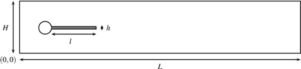
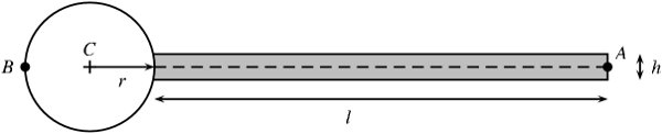
Figure 1. The domain for the FSI problem [27].

The fluid region is governed by the Navier-Stokes equations (8) with $\hbox{\boldmath$f$}^{f}=0$, and the elastic structure is governed by the equations for hyperelasticity (20) with $\hbox{\boldmath$f$}^{s}=0$. The coupling conditions (31a)–(31b) is used on the fluid-structure interface $\Gamma_{t}$, and the following boundary conditions are used:

• A parabolic velocity profile is prescribed at the left channel inflow

  $$\hbox{\boldmath$u$}^{f}(0,y,t)=\left\{\begin{tabular}[]{ll}$\hbox{\boldmath$u$}^{f}(0,y)\frac{1-\cos(\frac{\pi}{2}t)}{2}$&if $t<2$,\\[8.61108pt] $\hbox{\boldmath$u$}^{f}(0,y)$&otherwise,\end{tabular}\right.$$

  where $\hbox{\boldmath$u$}^{f}(0,y)=1.5\bar{U}\frac{y(H-y)}{({H}/{2})^{2}}=61.5\bar{U}\frac{4.0}{0.1681}{y(0.41-y)}$.

• The stress-free boundary condition $\hbox{\boldmath$\sigma$}^{f}\hbox{\boldmath$n$}=0$ is prescribed at the outflow.

• The no-slip condition ($\hbox{\boldmath$u$}^{f}=0$, or $\hbox{\boldmath$d$}=\hbox{\boldmath$u$}^{s}=0$) is prescribed on all the other boundary parts.

Two test cases resulting in time periodic solutions are considered, which are denoted as FSI2 and FSI3 in [27]. The associated material parameters are listed in Table 1.

parameter	$\rho^{s}[10^{3}\mathrm{\frac{kg}{m^{3}}}]$	$\lambda^{s}[10^{6}\mathrm{\frac{kg}{ms^{2}}}]$	$\mu^{s}[10^{6}\mathrm{\frac{kg}{ms^{2}}}]$	$\rho^{f}[10^{3}\mathrm{\frac{kg}{m^{3}}}]$	$\mu^{f}[\mathrm{\frac{kg}{ms}}]$	$\bar{U}[\mathrm{\frac{m}{s}}]$
FSI2	10	2.0	0.5	1	1	1
FSI3	1	8.0	2.0	1	1	2

Table 1. Parameter settings for the two test cases.

Quantities of interest are

• The displacement of the control point $A$ at the end of the beam structure (see Figure 1).

• The lift and drag forces acting on the cylinder and the beam structure:

  $$(F_{D},F_{L})=\int_{S}\hbox{\boldmath$\sigma$}^{f}\hbox{\boldmath$n$}\,\mathrm{ds},$$

  where $S$ denotes the boundary between the fluid domain and the cylinder together with the elastic structure.

We compare the computational results with the reference data provided in [7] after a fully developed periodic flow is formed.

5.2. Discretization

We apply Algorithm 1 to both test cases, and take the polynomial degree $k=3$ throughout. Three set of meshes are used in the simulation. The coarse mesh, which contains $495$ triangular elements, is generated automatically from the geometry by NETGEN [23]. Curved elements with polynomial degree $k=3$ are used for elements near the cylinder. The intermediate and fine meshes are obtained from the coarse mesh by uniform refinements. See Figure 2 for the coarse and intermediate meshes.

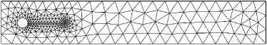
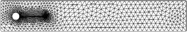
Figure 2. The computational meshes. Left: coarse mesh with 495 elements. Right: intermediate mesh with 1980 elements. Curved elements with polynomial degree $3$ are used near the cylinder.

The nonlinear system in (34) is solved via the Newton’s method where the iteration is terminated with an absolute tolerance of $10^{-8}$ for the $l_{2}$-norm of the residual vector. Static condensation is used for the resulting linear system problems, where the globally coupled degrees of freedom consists of only those lie on the mesh skeleton, namely, those for the normal-normal component of the fluid stress $\widetilde{\sigma}_{h}^{f}$, the tangential component of the fluid velocity $\widetilde{\hbox{\boldmath$u$}}_{h}^{f}$, the normal component of the structure velocity $\widetilde{\hbox{\boldmath$u$}}_{h}^{s}$, and the structure velocity $\hbox{\boldmath$u$}_{h}^{s}$ on the mesh skeleton. The globally coupled linear system is then solved via a sparse direct solver. We observe in average 4-6 iterations for the nonlinear solver to converge. The number of globally coupled degrees of freedom is $6188$ on the coarse mesh, $24256$ on the intermediate mesh, and $96032$ on the fine mesh.

For the FSI2 problem, we use three different time step size, namely, $\Delta t=0.02,0.01,0.005$, and stop the simulation at time $T=15$. A fully developed periodic flow is observed starting around time $t=10$. In Figure 3, we plot the quantities of interest for the fully developed flow over one second time for Algorithm 1 on the three meshes, along with reference data provided in [7]. Two comments are in order.

• On a fixed mesh, we observe a better phase and amplitude accuracy, compared with the reference data, when decreasing the time step size from $\Delta t=0.02$ (in red) to $\Delta t=0.01$ (in green). However, further decreasing the time step size to $\Delta t=0.005$ (in blue) does not lead to significantly better results.

• Comparing the results on different meshes when the time step size is fixed, we find the all results are very similar to each other. This indicates that our spatial discretization is very accurate even on the coarse mesh.

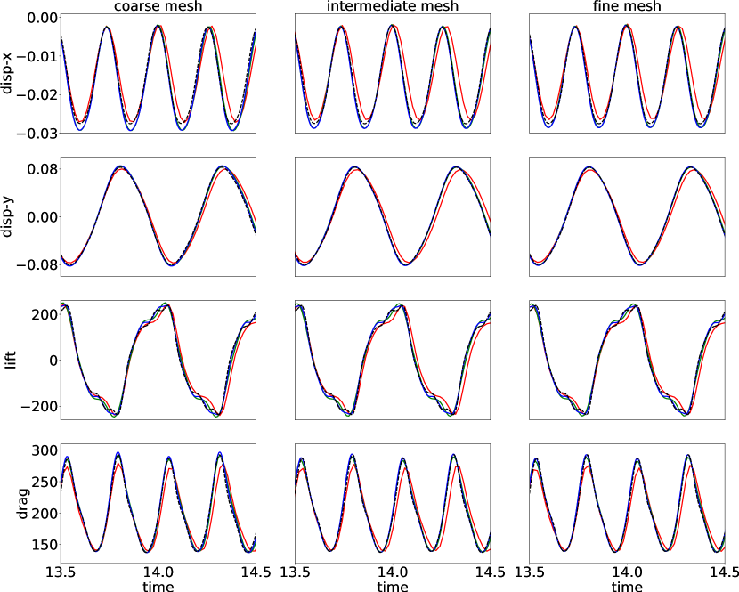
Figure 3. The quantities of interest for FSI2 in the fully developed flow regime. Left column: coarse mesh. Middle column: intermediate mesh. Right column: fine mesh. First row: $x$-component of displacement at point $A$. Second row : $y$-component of displacement at point $A$. Third row: lift force. Last row: drag force. Red line: $\Delta t=0.02$; Green line: $\Delta t=0.01$; Blue line: $\Delta t=0.005$; Dashed black line: reference solution from [7].

For the FSI3 problem, we use three different time step size, namely, $\Delta t=0.01,0.005,0.0025$, and stop the simulation at time $T=9$. A fully developed periodic flow is observed starting around time $t=5$. In Figure 4, we plot the computed quantities of interest for the fully developed flow over half second time. Overall, all the results are in very good agreements with the reference data. We make two more comments.

• Similar to the FSI2 case, on a fixed mesh, we observe a better phase and amplitude accuracy, compared with the reference data, when decreasing the time step size from $\Delta t=0.01$ (in red) to $\Delta t=0.005$ (in green). However, further decreasing the time step size to $\Delta t=0.0025$ (in blue) does not lead to better results.

• Comparing the results on different meshes when the time step size is fixed at $\Delta t=0.005$ (in green) or $\Delta t=0.0025$ (in blue), we find the results in the displacements and lift force are very similar on the intermediate and fine meshes, which are slightly better than those on the coarse mesh. While the results in the drag force on the fine mesh is still the most accurate, those on the coarse mesh is surprisingly better than those on the intermediate mesh, which slightly underestimate the magnitude by about $1\%$.

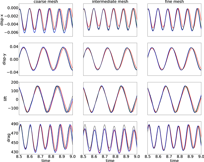
Figure 4. The quantities of interest for FSI3 in the fully developed flow regime. Left column: coarse mesh. Middle column: intermediate mesh. Right column: fine mesh. First row: $x$-component of displacement at point $A$. Second row : $y$-component of displacement at point $A$. Third row: lift force. Last row: drag force. Red line: $\Delta t=0.02$; Green line: $\Delta t=0.01$; Blue line: $\Delta t=0.005$; Dashed black line: reference solution from [7].

6. Conclusion

We have presented a novel coupled HDG scheme for the FSI problem, where the moving domain fluid Navier-Stokes equations are solved using an ALE-divergence-free HDG scheme, and the equations for nonlinear elasticity is solved in the Lagrangian framework using a novel $H(\mathrm{curl})$-conforming HDG scheme. Numerical results on the benchmark problem of Turek and Hron [27] showed good performance of our method. Our ongoing work consists of (1) the construction of good preconditioners for the linearized problems, and (2) the construction of efficient, robust and accurate partitioned algorithms for this HDG scheme.

References

- [1] D. Boffi, F. Brezzi, and M. Fortin, Mixed finite element methods and applications, vol. 44 of Springer Series in Computational Mathematics, Springer, Heidelberg, 2013.
- [2] H.-J. Bungartz and M. Schäfer, Fluid-structure interaction: modelling, simulation, optimisation, vol. 53, Springer Science & Business Media, 2006.
- [3] S. K. Chakrabarti, Numerical models in fluid-structure interaction, WIT, 2005.
- [4] B. Cockburn and G. Fu, Devising superconvergent HDG methods with symmetric approximate stresses for linear elasticity by -decompositions, IMA J. Numer. Anal., 38 (2018), pp. 566–604.
- [5] B. Cockburn, G. Fu, and W. Qiu, Discrete -inequalities for spaces admitting M-decompositions, SIAM J. Numer. Anal., 56 (2018), pp. 3407–3429.
- [6] E. H. Dowell and K. C. Hall, Modeling of fluid-structure interaction, Annual review of fluid mechanics, 33 (2001), pp. 445–490.
- [7] FEATFLOW, Finite element software for the incompressible navier-stokes equations, www.featflow.de.
- [8] G. Fu, Arbitrary Lagrangian–Eulerian hybridizable discontinuous Galerkin methods for incompressible flow with moving boundaries and interfaces, Comput. Methods Appl. Mech. Engrg., 367 (2020), p. 113158.
- [9] G. Fu, Y. Jin, and W. Qiu, Parameter-free superconvergent -conforming HDG methods for the Brinkman equations, IMA J. Numer. Anal., 39 (2019), pp. 957–982.
- [10] F. Fuentes, B. Keith, L. Demkowicz, and S. Nagaraj, Orientation embedded high order shape functions for the exact sequence elements of all shapes, Comput. Math. Appl., 70 (2015), pp. 353–458.
- [11] G. Hou, J. Wang, and A. Layton, Numerical methods for fluid-structure interaction—a review, Communications in Computational Physics, 12 (2012), pp. 337–377.
- [12] C. Lehrenfeld, Hybrid Discontinuous Galerkin methods for solving incompressible flow problems. Diploma Thesis, MathCCES/IGPM, RWTH Aachen, 2010.
- [13] C. Lehrenfeld and J. Schöberl, High order exactly divergence-free hybrid discontinuous Galerkin methods for unsteady incompressible flows, Comput. Methods Appl. Mech. Engrg., 307 (2016), pp. 339–361.
- [14] M. Neunteufel, A. Pechstein, and J. Schöberl, Three-field mixed finite element methods for nonlinear elasticity, 2020.
- [15] M. Neunteufel and J. Schöberl, Fluid-structure interaction with h(div)-conforming finite elements, Computers & Structures, 243 (2021), p. 106402.
- [16] F. Nobile, Numerical approximation of fluid-structure interaction problems with application to haemodynamics, PhD thesis, École polytechnique fédérale de Lausanne, 2001.
- [17] A. Pechstein and J. Schöberl, Tangential-displacement and normal-normal-stress continuous mixed finite elements for elasticity, Math. Models Methods Appl. Sci., 21 (2011), pp. 1761–1782.
- [18] , Anisotropic mixed finite elements for elasticity, Internat. J. Numer. Methods Engrg., 90 (2012), pp. 196–217.
- [19] A. S. Pechstein and J. Schöberl, The TDNNS method for Reissner-Mindlin plates, Numer. Math., 137 (2017), pp. 713–740.
- [20] A. Quaini, Algorithms for Fluid-Structure Interaction Problems Arising in Hemodynamics, PhD thesis, École polytechnique fédérale de Lausanne, 2009.
- [21] T. Richter, Fluid-structure interactions: models, analysis and finite elements, vol. 118, Springer, 2017.
- [22] S. Zaglmayr, High order finite element methods for electromagnetic field computation, 2006. PhD thesis, Johannes Kepler Universit ät Linz, Linz.
- [23] J. Schöberl, NETGEN An advancing front 2D/3D-mesh generator based on abstract rules, Comput Visual Sci, 1 (1997), pp. 41–52.
- [24] J. Schöberl, C++11 Implementation of Finite Elements in NGSolve, 2014. ASC Report 30/2014, Institute for Analysis and Scientific Computing, Vienna University of Technology.
- [25] A. Shamanskiy and B. Simeon, Mesh moving techniques in fluid-structure interaction: robustness, accumulated distortion and computational efficiency, Computational Mechanics, 67 (2021), pp. 583–600.
- [26] S. Terrana, N. C. Nguyen, J. Bonet, and J. Peraire, A hybridizable discontinuous Galerkin method for both thin and 3D nonlinear elastic structures, Comput. Methods Appl. Mech. Engrg., 352 (2019), pp. 561–585.
- [27] S. Turek and J. Hron, Proposal for numerical benchmarking of fluid-structure interaction between an elastic object and laminar incompressible flow, in Fluid-structure interaction, vol. 53 of Lect. Notes Comput. Sci. Eng., Springer, Berlin, 2006, pp. 371–385.
- [28] K. Washizu, Variational methods in elasticity and plasticity, Pergamon Press, Oxford-New York-Toronto, Ont., second ed., 1975. With a foreword by R. L. Bisplinghoff, International Series of Monographs in Aeronautics and Astronautics, Division I: Solid and Structural Mechanics, Vol. 9.
- [29] T. Wick, Fluid-structure interactions using different mesh motion techniques, Comput. Struct., 89 (2011), pp. 1456–1467.