The Josephson-Anderson Relation and the Classical D’Alembert Paradox

Abstract

Generalizing prior work of P. W. Anderson and E. R. Huggins, we show that a “detailed Josephson-Anderson relation” holds for drag on a finite body held at rest in a classical incompressible fluid flowing with velocity ${\bf V}.$ The relation asserts an exact equality between the instantaneous power consumption by the drag, $-{\bf F}{\mbox{\boldmath$\cdot$}}{\bf V},$ and the vorticity flux across the potential mass current, $-(1/2)\int dJ\int\epsilon_{ijk}\Sigma_{ij}\,d\ell_{k}.$ Here $\Sigma_{ij}$ is the flux in the $i$th coordinate direction of the conserved $j$th component of vorticity and the line-integrals over $\ell$ are taken along streamlines of the potential flow solution ${\bf u}_{\phi}={\mbox{\boldmath$\nabla$}}\phi$ of the ideal Euler equation, carrying mass flux $dJ=\rho\,{\bf u}_{\phi}{\mbox{\boldmath$\cdot$}}d{\bf A}.$ The results generalize the theories of M. J. Lighthill for flow past a body and, in particular, the steady-state relation $(1/2)\epsilon_{ijk}\langle\Sigma_{jk}\rangle=\partial_{i}\langle h\rangle,$ where $h=p+(1/2)|{\bf u}|^{2}$ is the generalized enthalpy or total pressure, extends Lighthill’s theory of vorticity generation at solid walls into the interior of the flow. We use these results to explain drag on the body in terms of vortex dynamics, unifying the theories for classical fluids and for quantum superfluids. The results offer a new solution to the “D’Alembert paradox” at infinite Reynolds numbers and imply the necessary conditions for turbulent drag reduction.

I Introduction

The origin of the Josephson-Anderson relation lies in the work of Josephson on tunneling of Cooper pairs through normal-superconductor metal junctions and, in particular, his AC effect Josephson (1962). However, the relation assumed its most elegant and powerful statement in the seminal paper of Anderson on flow in superfluid ${\,\!}^{4}$He Anderson (1966). The relation has had sufficient sustained importance that it garnered two extensive reviews, thirty years Packard (1998) and fifty years Varoquaux (2015) after Anderson’s original work. In its most basic form, it relates the time-derivative of the phase $\theta$ of the superfluid macroscopic wavefunction and the chemical potential $\mu$ as

$$\hbar\frac{d\theta}{dt}=-\left(\mu+\frac{1}{2}m|{\bf u}|^{2}\right)$$ (I.1)

where ${\bf u}=\hbar{\mbox{\boldmath$\nabla$}}\theta/m$ is the superfluid velocity. A special significance holds for this relation because topological phase-defects exist in superfluids as discrete vortex lines with circulation quantized in units of $h/m$ Onsager (1949a); Feynman (1955). The importance of the Josephson-Anderson relation arises from the intimate connection it reveals between force balance and vortex motion. This connection can already be understood by applying a space-gradient to Eq.(I.1) which yields the equation of motion for the superfluid velocity

$$\frac{d{\bf u}}{dt}=\partial_{t}{\bf u}+({\bf u}{\mbox{\boldmath$\cdot$}}{\mbox{\boldmath$\nabla$}}){\bf u}=-(1/m){\mbox{\boldmath$\nabla$}}\mu$$ (I.2)

A superfluid would be expected to flow without any applied chemical potential gradient (or pressure-gradient, for the incompressible isothermal limit), but Anderson showed that a drop in chemical potential would occur if there were a time-average flux of quantized vortices across the streamlines of the potential superfluid flow Anderson (1966). See also Josephson Josephson (1965) for the corresponding effect of voltage drop in superconductors.

A significant extension of these ideas was obtained subsequently by Huggins Huggins (1970a) whose “detailed Josephson equation” was further able to relate vortex motion to energy dissipation. See also Zimmermann (1993); Greiter (2005); Varoquaux (2015) for alternative derivations of Huggins’ result. Such vortex motion by “$2\pi$-phase slips” has been for many years the standard paradigm for energy dissipation in low-temperature superfluids and superconductors Bishop et al. (1993). Furthermore, because Huggins’ detailed relation was derived without any sort of averaging, it could be applied to individual flow realizations and it was found to yield deep insight into otherwise very complicated vortex dynamics. We may quote from the review of Packard, who wrote that

“the equation provides an elegant short cut to certain predictions … that involve the complex motion of quantized vortices. These same predictions by other methods require a detailed knowledge of vortex motion and involve considerable computational effort.” Packard (1998)

The reviews Packard (1998); Varoquaux (2015) both analyzed a large number of concrete examples to justify the remarkable efficacy of the detailed Josephson-Anderson relation to understand and predict complex superfluid vortex dynamics.

That classical fluids should satisfy a similar relation was already understood by Anderson, who devoted Appendix B of his 1966 article to deriving an analogous result for classical hydrodynamics Anderson (1966). He stated that he had been unable to find the same result written anywhere in the literature and conjectured that “it was understood by the ‘classics’ but is of no value in classical hydrodynamics so was never stated” . Most superfluid physicists have followed Anderson in discounting any significance of the Josephson-Anderson relation for classical fluids. As a typical statement, we may quote from the recent review article of Varoquaux:

“This result is of no special importance in classical hydrodynamics because the velocity circulation carried by each vortex, albeit constant, can take any value, while in the superfluid it is directly related to the phase of the macroscopic wave function and quantized.” Varoquaux (2015)

A notable exception to this trend was Huggins, whose original paper Huggins (1970a) already demonstrated the validity of his “detailed relation” for classical viscous Navier-Stokes solutions and who later wrote a paper applying his results to classical turbulent channel flow Huggins (1994) .

Unrecognized by Anderson and the rest of the superfluid community, however, there were already important applications of closely related ideas in classical hydrodynamics. A very early foreshadowing was work on turbulent pipe flow by Taylor Taylor (1932), who realized that pressure-drop down the pipe implies transverse vortex motion but who did not pursue the connection further. More important was a seminal work of Lighthill Lighthill (1963), who presented a very broad vision of classical fluid mechanics from the perspective of vortex dynamics, encompassing laminar, transitional and fully turbulent flow. Just three years before Anderson’s work on superfluids, Lighthill argued that vorticity flux from solid walls is fundamentally due to tangential pressure gradients at the wall and he presented many important applications of this principle to classical incompressible fluid dynamics. In fact, his ideas are closely related to those of Huggins Huggins (1970b, a, 1971, 1994), which naturally extend Lighthill’s concept of vorticity flux at solid walls into the the interior of the flow. These connections were previously discussed by us in a paper on turbulent channel flow Eyink (2008), which further developed Huggins ideas on that problem and put them in the context of contemporary work on the “attached-eddy hypothesis”.

In this paper we present a new application of the classical Josephson-Anderson relation to flow past a finite, solid body and to the problem of the origin of drag. This is in some ways a much more illuminating application of the relation, although it requires some significant modification of the analysis both of Huggins and of Lighthill. In fact, Lighthill in his paper Lighthill (1963) had discussed this same problem in the rest frame of the fluid, appealing there to Kelvin’s minimum-energy theorem Kelvin (1882). We shall see that this theorem does not hold in the body frame, and this fact crucially enters into the analysis. Kelvin’s theorem involves the unique potential flow solution of the inviscid Euler equation satisfying the no-flow-through condition at the body surface, which, according to the famous result of d’Alembert predicts zero drag around a moving body d’Alembert (1749, 1768); Grimberg et al. (2008). In superfluids this is no “paradox” but is instead a physically observable phenomenon when the body moves at low speeds below a critical velocity. The origin of superfluid drag above this critical velocity was the subject of a study by Frisch, Pomeau and Rica Frisch et al. (1992), which spawned a substantial following literature up to the present time, e.g. Jackson et al. (1998); Winiecki et al. (1999, 2000); Winiecki and Adams (2000); Winiecki (2001); Huepe and Brachet (2000); Nore et al. (2000); Sasaki et al. (2010); Stagg et al. (2014, 2015); Musser et al. (2019). Our analysis will demonstrate a deep similarity between the origin of drag in classical and quantum fluids, with the Josephson-Anderson relation providing the key unifying concept. Although we shall focus mainly on the classical case, we shall make various remarks as we proceed concerning differences and similarities with the quantum case. Our approach applies to classical flows at any Reynolds number but in particular extends to the infinite-Reynolds turbulent regime, making a connection of the D’Alembert paradox with the Onsager theory of dissipative Euler solutions Onsager (1949b); Eyink and Sreenivasan (2006); Eyink (2018).

II Concise Review of Theories of Huggins and Lighthill

We begin with a very brief review of the essential ideas in the theories of Huggins Huggins (1970b, a, 1971, 1994) and Lighthill Lighthill (1963).

Although we shall be principally concerned with simple fluids described by the incompressible Navier-Stokes equation at constant density $\rho,$ the ideas of Huggins apply to an extended system of equations with additional accelerations, due to forces both conservative $-{\mbox{\boldmath$\nabla$}}U$ for a potential $U$ and non-conservative ${\bf g}$ with ${\mbox{\boldmath$\nabla$}}{\mbox{\boldmath$\times$}}{\bf g}\neq{\mbox{\boldmath$0$}}$, written in the form:

$$\partial_{t}{\bf u}={\bf u}{\mbox{\boldmath$\times$}}{\mbox{\boldmath$\omega$}}-\nu{\mbox{\boldmath$\nabla$}}{\mbox{\boldmath$\times$}}{\mbox{\boldmath$\omega$}}-{\bf g}-{\mbox{\boldmath$\nabla$}}\left(p+U+\frac{1}{2}|{\bf u}|^{2}\right),$$ (II.1)

where $p=P/\rho$ is kinematic pressure and $\nu=\eta/\rho$ is kinematic viscosity. For example, $U$ could be a gravitational or electrostatic potential and ${\bf g}$ could arise from the stress of a polymer additive. Huggins Huggins (1971, 1994) observed that equations of the above class can be rewritten component-wise as

$$\partial_{t}u_{i}=\frac{1}{2}\epsilon_{ijk}\Sigma_{jk}-\partial_{i}h$$ (II.2)

in terms of an anti-symmetric tensor

$$\Sigma_{ij}=u_{i}\omega_{j}-u_{j}\omega_{i}+\nu\left(\frac{\partial\omega_{i}}{\partial x_{j}}-\frac{\partial\omega_{j}}{\partial x_{i}}\right)-\epsilon_{ijk}g_{k}$$ (II.3)

and a generalized enthalpy or total pressure (static pressure plus dynamic pressure)

$$h=p+U+\frac{1}{2}|{\bf u}|^{2}.$$ (II.4)

The meaning of the tensor $\Sigma$ is discovered by taking the curl of equation (II.1) to obtain the analogue of the Helmholtz equation for conservation of vorticity

$$\partial_{t}{\mbox{\boldmath$\omega$}}+{\mbox{\boldmath$\nabla$}}{\mbox{\boldmath$\cdot$}}{\mbox{\boldmath$\Sigma$}}={\mbox{\boldmath$0$}}$$ (II.5)

with $\Sigma_{ij}$ representing the flux of the $j$th component of vorticity in the $i$th coordinate direction. For this reason, we shall refer to $\Sigma$ as the Huggins vorticity-flux tensor.

The various terms in Eq.(II.3) have transparent physical meanings, with the first representing advective transport, the second transport by vortex-stretching/tilting, the third term in parentheses viscous transport and the final term a flux by the Magnus effect transverse to the applied force. The rewriting of the momentum conservation equation in the form (II.2) is the classical Josephson-Anderson relation in its simplest version. It implies, for example, that for a steady solution or for a suitable time-average $\langle\cdot\rangle$ (average over a period for an oscillatory solution or long-time ergodic average for a chaotic solution) the mean gradients of $h$ and the mean vorticity fluxes are exactly related by

$$\frac{1}{2}\epsilon_{ijk}\langle\Sigma_{jk}\rangle=\partial_{i}\langle h\rangle.$$ (II.6)

Thus, a mean gradient of $h$ must always be associated to a transverse vorticity flux, and vice versa.

Furthermore, Huggins Huggins (1970b, a) (and see also Eyink (2008), Appendix B) derived a less obvious result, the “detailed Josephson relation”, in the case of a generalized channel flow, as pictured in Figure 1. Here the fluid velocity is assumed to be specified on the in-flow surface $S_{in},$ out-flow surface $S_{out},$ and at the channel wall $S_{w}$ as

$$\left.{\bf u}\right|_{S_{in}}={\bf u}_{in},\quad\left.{\bf u}\right|_{S_{out}}={\bf u}_{out},\quad\left.{\bf u}\right|_{S_{w}}={\mbox{\boldmath$0$}}$$ (II.7)

As in the proof of the Kelvin minimum energy theorem (Kelvin (1882); Lamb (1945), Art.45; Batchelor (2000),§6.2; Wu et al. (2007), §2.4.4), Huggins then introduced the unique incompressible potential flow ${\bf u}_{\phi}={\mbox{\boldmath$\nabla$}}\phi$ satisfying the same boundary conditions:

$$\left.{\bf u}_{\phi}\right|_{S_{in}}={\bf u}_{in},\quad\left.{\bf u}_{\phi}\right|_{S_{out}}={\bf u}_{out},\quad\left.{\bf u}_{\phi}\right|_{S_{w}}={\mbox{\boldmath$0$}}$$ (II.8)

and the complementary field ${\bf u}_{\omega}={\bf u}-{\bf u}_{\phi}$ which represents the velocity due to vorticity. It then easily follows that ${\bf u}_{\phi}$ and ${\bf u}_{\omega}$ are orthogonal

$$\int_{\Omega}{\bf u}_{\phi}{\mbox{\boldmath$\cdot$}}{\bf u}_{\omega}\,dV=\int_{\Omega}{\mbox{\boldmath$\nabla$}}\cdot(\phi{\bf u}_{\omega})\,dV=\int_{\partial\Omega}\phi({\bf u}_{\omega}{\mbox{\boldmath$\cdot$}}\hat{{\bf n}})\,dA=0$$ (II.9)

which is the essence of Kelvin’s theorem. Using this orthogonality, Huggins was able to derive equations for energies in the potential flow $E_{\phi}=(\rho/2)\int_{\Omega}|{\bf u}_{\phi}|^{2}dV$ and in the rotational flow $E_{\omega}=(\rho/2)\int_{\Omega}|{\bf u}_{\omega}|^{2}dV$ as

$$\frac{dE_{\phi}}{dt}=\int dJ(h_{in}-h_{out})-{\mathcal{T}}$$ (II.10)

and

$$\frac{dE_{\omega}}{dt}={\mathcal{T}}-\int_{\Omega}[\eta|{\mbox{\boldmath$\omega$}}|^{2}+\rho{\bf u}{\mbox{\boldmath$\cdot$}}{\bf g}]\,dV$$ (II.11)

with

$${\mathcal{T}} = -\rho\int{\bf u}_{\phi}{\mbox{\boldmath$\cdot$}}({\bf u}{\mbox{\boldmath$\times$}}{\mbox{\boldmath$\omega$}}-\nu{\mbox{\boldmath$\nabla$}}{\mbox{\boldmath$\times$}}{\mbox{\boldmath$\omega$}}-{\bf g})\,dV$$ (II.12)

$$= -\int dJ\int({\bf u}{\mbox{\boldmath$\times$}}{\mbox{\boldmath$\omega$}}-\nu{\mbox{\boldmath$\nabla$}}{\mbox{\boldmath$\times$}}{\mbox{\boldmath$\omega$}}-{\bf g}){\mbox{\boldmath$\cdot$}}\,d{\mbox{\boldmath$\ell$}}$$ (II.13)

$$= -\frac{1}{2}\int dJ\int\epsilon_{ijk}\Sigma_{ij}\,d\ell_{k}$$ (II.14)

Here the line integrals are along streamlines of the potential flow and $dJ=\rho{\bf u}_{\phi}{\mbox{\boldmath$\cdot$}}d{\bf A}$ is the element of mass flux along each streamline, with ${\mathcal{T}}$ representing transfer of energy from potential to rotational flow by flux of vorticity across mass current. As a consequence of Eq.(II.10), Huggins then obtained the “detailed Josephson relation”

$${\mathcal{T}}=\int dJ(h_{in}^{\prime}-h_{out}^{\prime})$$ (II.16)

with $h^{\prime}=h+\dot{\phi},$ which implies an instantaneous equality between energy transfer rate and work done by the total pressure field $h^{\prime}.$ Note that energy dissipation due to viscosity and other non-potential forces removes energy only from the rotational motions. See Appendix A for a brief, self-contained derivation of Huggins’ result.

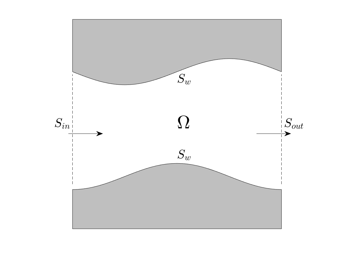
Figure 1: Flow through a channel $\Omega$ with in-flow surface $S_{in},$ out-flow surface $S_{out},$ and channel walls $S_{w}$

The velocity decomposition introduced by Huggins is very natural for superfluids, where ${\bf u}_{\phi}$ represents the ground-state superfluid velocity and ${\bf u}_{\omega}$ the (incompressible) vortical excitations such as vortex rings. As we shall see in Section III.2, Lighthill Lighthill (1963) introduced the identical decomposition in his discussion of flow around a solid body, using quite different arguments. Furthermore, Lighthill recognized that there would be a creation of vorticity at solid walls with a normal flux $\sigma$ related exactly to Huggins’ vorticity flux tensor, as

$${\mbox{\boldmath$\sigma$}}=\hat{{\bf n}}{\mbox{\boldmath$\cdot$}}{\mbox{\boldmath$\Sigma$}}=\hat{{\bf n}}{\mbox{\boldmath$\times$}}\nu({\mbox{\boldmath$\nabla$}}{\mbox{\boldmath$\times$}}{\mbox{\boldmath$\omega$}})+\hat{{\bf n}}{\mbox{\boldmath$\times$}}{\bf g},$$ (II.17)

which is now called the Lighthill vorticity source. In fact, Lighthill wrote his source explicitly for a flat wall only, and the general formula above for a curved wall was first proposed by Lyman Lyman (1990). There is more than one possible generalization of Lighthill’s flat-wall expression to curved walls (e.g. see Panton (1984); Wu and Wu (1993, 1996, 1998)), but Lyman’s proposal is uniquely the one that corresponds to creation of circulation at the boundary (Eyink (2008), Appendix A). Lighthill Lighthill (1963) further realized that vorticity generation at the wall could be related to tangential pressure gradients, as can be seen by substituting the equation of motion (II.1) into (II.17), to obtain

$${\mbox{\boldmath$\sigma$}}=-\hat{{\bf n}}\times({\mbox{\boldmath$\nabla$}}h+\partial_{t}{\bf u}).$$ (II.18)

Here we have included the term $\partial_{t}{\bf u},$ which is non-zero if the wall is accelerating tangential to itself, that was first introduced by Morton Morton (1984), who also emphasized the inviscid nature of vorticity generation according to formula (II.18). In common with Josephson and Anderson, Lighthill Lighthill (1963) thus realized also that pressure gradients and transverse vorticity fluxes are inextricably linked.

III The Classical Josephson-Anderson Relation for a Finite Moving Body

In this section we present the derivation of the new Josephson-Anderson relation for flow around a body, which requires extended mathematical discussion. However, a reader who is most interested in concrete applications can skip directly to section IV where flow around a sphere is considered in detail as an illustrative example.

III.1 Set-Up of the Problem

We consider the flow around a finite solid body $B$ with smooth boundary $\partial B,$ held at rest, in an incompressible fluid that is filling the region $\Omega={\mathbb{R}}^{3}\backslash B$ and moving at constant velocity ${\it{\bf V}}={\rm V}\hat{{\bf x}}$ upstream of the body and at far distances from it. See Figure 2. By Galilean invariance, we can equivalently consider the body to be in translational motion with velocity $-{\rm V}\hat{{\bf x}}$ through a fluid at rest and that point of view is sometimes more convenient. In this flow set-up we shall consider the solution ${\bf u}$ of the viscous incompressible Navier-Stokes equation

$$\partial_{t}{\bf u}+{\mbox{\boldmath$\nabla$}}{\mbox{\boldmath$\cdot$}}\left({\bf u}{\bf u}+p{\bf I}-2\nu{\bf S}\right)={\mbox{\boldmath$0$}},\quad{\mbox{\boldmath$\nabla$}}{\mbox{\boldmath$\cdot$}}{\bf u}=0$$ (III.1)

with the boundary conditions

$$\left.{\bf u}\right|_{\partial B}={\mbox{\boldmath$0$}},\quad{\bf u}\underset{|{\bf x}|\to\infty}{\sim}{\bf V}.$$ (III.2)

Note that in Eq.(III.1) we have written the Navier-Stokes equation as a local conservation law for linear momentum, with the total stress tensor (in dyadic notation)

$${\bf T}={\bf u}{\bf u}+p{\bf I}-2\nu{\bf S}$$ (III.3)

where ${\bf S}=\frac{1}{2}[({\mbox{\boldmath$\nabla$}}{\bf u})+({\mbox{\boldmath$\nabla$}}{\bf u})^{\top}]$ is the strain-rate tensor. We shall assume here that the Navier-Stokes solutions are smooth for all times.

For comparison, we shall also consider the potential-flow solution of the incompressible Euler equation

$$\partial_{t}{\bf u}_{\phi}+{\mbox{\boldmath$\nabla$}}{\mbox{\boldmath$\cdot$}}\left({\bf u}_{\phi}{\bf u}_{\phi}+p_{\phi}{\bf I}\right)={\mbox{\boldmath$0$}},\quad{\mbox{\boldmath$\nabla$}}{\mbox{\boldmath$\cdot$}}{\bf u}_{\phi}=0$$ (III.4)

with ${\bf u}_{\phi}={\mbox{\boldmath$\nabla$}}\phi$ given by a velocity potential $\phi$ which satisfies the boundary conditions

$$\left.\frac{\partial\phi}{\partial n}\right|_{\partial B}=0,\quad\phi\underset{|{\bf x}|\to\infty}{\sim}{\rm V}x$$ (III.5)

Standard theory of potential flow implies that there is a unique, smooth solution with potential $\phi$ satisfying the Laplace equation $\triangle\phi=0$ for b.c. (III.5) and with kinematic pressure given by the Bernoulli equation

$$\partial_{t}\phi+\frac{1}{2}|{\bf u}_{\phi}|^{2}+p_{\phi}=0.$$ (III.6)

Here the pressure $p_{\phi}$ has been assumed for convenience to equal the constant value $-\frac{1}{2}{\rm V}^{2}$ at infinity. This potential flow is, of course, the subject of the famous D’Alembert paradox d’Alembert (1749); Grimberg et al. (2008) according to which the force exerted by the fluid on the body

$${\bf F}_{\phi}=-\int_{\partial B}P_{\phi}\,\hat{{\bf n}}\,dA$$ (III.7)

has vanishing drag, or ${\bf V}{\mbox{\boldmath$\cdot$}}{\bf F}_{\phi}=0.$ Note in Eq.(III.7) and hereafter that $\hat{{\bf n}}$ denotes the normal at the surface $\partial B$ pointing from the solid body into the fluid.

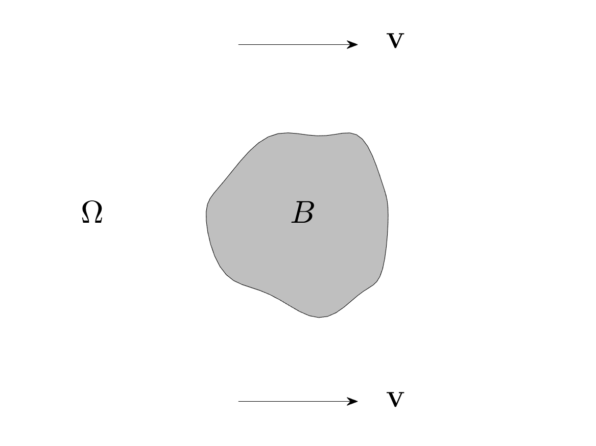
Figure 2: Flow around a finite body $B$ in an unbounded region $\Omega$ filled with fluid moving at a velocity ${\bf V}$ at far distances.

III.2 Potential/Vortical Representation of Navier-Stokes

Following the approach of Huggins Huggins (1970a) to derive the Josephson-Anderson relation, we introduce the corresponding rotational contributions by the definitions

$${\bf u}_{\omega}:={\bf u}-{\bf u}_{\phi},\quad p_{\omega}:=p-p_{\phi}.$$ (III.8)

Although the Navier-Stokes velocity field is thereby decomposed as ${\bf u}={\mbox{\boldmath$\nabla$}}\phi+{\mbox{\boldmath$\nabla$}}{\mbox{\boldmath$\times$}}{\mbox{\boldmath$\psi$}}_{\omega}$ into gradient and curl parts, this is not the familiar Helmholtz decomposition. Recall that the Helmholtz decomposition for a piecewise smooth vector field ${\bf v}$ which is zero inside $B$ and smooth in the external flow domain $\Omega$ takes the form:

$${\bf v}({\bf x})=-{\mbox{\boldmath$\nabla$}}\left(\int_{\Omega}\frac{({\mbox{\boldmath$\nabla$}}{\mbox{\boldmath$\cdot$}}{\bf v})({\bf x}^{\prime})}{4\pi|{\bf x}-{\bf x}^{\prime}|}dV^{\prime}+\int_{\partial B}\frac{\hat{{\bf n}}{\mbox{\boldmath$\cdot$}}{\bf v}({\bf x}^{\prime})}{4\pi|{\bf x}-{\bf x}^{\prime}|}dA^{\prime}\right)$$ (III.9)

$$+{\mbox{\boldmath$\nabla$}}{\mbox{\boldmath$\times$}}\left(\int_{\Omega}\frac{({\mbox{\boldmath$\nabla$}}{\mbox{\boldmath$\times$}}{\bf v})({\bf x}^{\prime})}{4\pi|{\bf x}-{\bf x}^{\prime}|}dV^{\prime}+\int_{\partial B}\frac{\hat{{\bf n}}{\mbox{\boldmath$\times$}}{\bf v}({\bf x}^{\prime})}{4\pi|{\bf x}-{\bf x}^{\prime}|}dA^{\prime}\right)$$ (III.10)

(III.11)

See Kustepeli (2016) for an engaging discussion of the history of the Helmholtz decomposition and a useful survey of the mathematical literature, and see also Vladimirov (1977) for application to Navier-Stokes solutions outside a solid body. It is important to emphasize that the Helmholtz decomposition cannot be used to obtain uniquely the solenoidal velocity field ${\bf u}$ corresponding to a given vorticity field $\omega$ in $\Omega$ without specifying appropriate boundary conditions at $\partial B$ and, furthermore, that arbitrary boundary conditions cannot be imposed. Applied to a Navier-Stokes solution ${\bf u}$ with b.c. (III.2), the Helmholtz decomposition yields

$${\bf u}({\bf x},t)={\mbox{\boldmath$\nabla$}}{\mbox{\boldmath$\times$}}\left(\int_{\Omega}\frac{{\mbox{\boldmath$\omega$}}({\bf x}^{\prime},t)}{4\pi|{\bf x}-{\bf x}^{\prime}|}dV^{\prime}\right)$$ (III.12)

As already noted by Lighthill, “there is only a restricted class of vorticity distributions that correspond to real flows satisfying also the no-slip condition” Lighthill (1963).

The velocity field (III.12) is not, however, the only one that yields the vorticity distribution ${\mbox{\boldmath$\omega$}}={\mbox{\boldmath$\nabla$}}{\mbox{\boldmath$\times$}}{\bf u}.$ As also noted by Lighthill, “for any given solenoidal distribution of vorticity $\omega$ outside the body (whose motion is again prescribed), one and only one solenoidal velocity field exists, tending to zero at infinity and with zero normal velocity relative to the surface” Lighthill (1963). In fact, this unique velocity field mentioned by Lighthill for the Navier-Stokes solution ${\bf u}$ is exactly the field ${\bf u}_{\omega}$ defined in (III.8), which by its definition satisfies the boundary conditions

$$\left.\hat{{\bf n}}{\mbox{\boldmath$\cdot$}}{\bf u}_{\omega}\right|_{\partial B}=0, \left.\hat{{\bf n}}{\mbox{\boldmath$\times$}}{\bf u}_{\omega}\right|_{\partial B}=-\left.\hat{{\bf n}}{\mbox{\boldmath$\times$}}{\bf u}_{\phi}\right|_{\partial B}$$ (III.13)

$${\bf u}_{\omega} \underset{|{\bf x}|\to\infty}{\sim} {\mbox{\boldmath$0$}},$$ (III.15)

as a consequence of (III.2),(III.5). The Helmholtz decomposition for this velocity field ${\bf u}_{\omega}$ yields the representation

$${\bf u}_{\omega}({\bf x},t)={\mbox{\boldmath$\nabla$}}{\mbox{\boldmath$\times$}}\left(\int_{\Omega}\frac{{\mbox{\boldmath$\omega$}}({\bf x}^{\prime},t)}{4\pi|{\bf x}-{\bf x}^{\prime}|}dV^{\prime}+\int_{\partial B}\frac{\hat{{\bf n}}{\mbox{\boldmath$\times$}}{\bf u}_{\omega}({\bf x}^{\prime},t)}{4\pi|{\bf x}-{\bf x}^{\prime}|}dA^{\prime}\right)$$ (III.16)

and likewise the Euler solution ${\bf u}_{\phi}$ is given by

$${\bf u}_{\phi}({\bf x},t)={\mbox{\boldmath$\nabla$}}{\mbox{\boldmath$\times$}}\left(\int_{\partial B}\frac{\hat{{\bf n}}{\mbox{\boldmath$\times$}}{\bf u}_{\phi}({\bf x}^{\prime},t)}{4\pi|{\bf x}-{\bf x}^{\prime}|}dA^{\prime}\right),$$ (III.17)

which is an alternative representation of the potential flow as ${\bf u}_{\phi}={\mbox{\boldmath$\nabla$}}{\mbox{\boldmath$\times$}}{\mbox{\boldmath$\psi$}}_{\phi}$ in terms of a vector potential.

The quantities $\hat{{\bf n}}{\mbox{\boldmath$\times$}}{\bf u}_{\omega},$ $\hat{{\bf n}}{\mbox{\boldmath$\times$}}{\bf u}_{\phi}$ in the integral representations (III.16),(III.17) have a simple physical interpretation as singular vorticity sheets on the surface $\partial B,$ equal and opposite to each other. This observation allows us to identify the fields ${\bf u}_{\omega},$ ${\bf u}_{\phi}$ introduced by Huggins Huggins (1970a) with corresponding fields that appear in Lagrangian vortex methods for solving the Navier-Stokes equation, which were pioneered by Payne Payne (1956, 1958) and advocated by Lighthill Lighthill (1963). These methods have since been substantially developed with many alternative schemes proposed. See Ploumhans et al. (2002) for a clear discussion of the application to flow around a solid body and see Branlard (2017) for a recent general review. In the version explained by Lighthill Lighthill (1963), given a vorticity distribution $\omega$ in $\Omega$ at each instant (obtained by advecting, stretching and diffusing the prior distribution), one uses the Biot-Savart formula to construct the unique solenoidal velocity field which is vanishing at infinity and satisfying no-flow-through conditions at $\partial B,$ which is the field ${\bf u}_{\omega}.$ However, this velocity field does not satisfy the stick b.c at $\partial B$ on its tangential components and, also, it is not a constant velocity ${\bf V}$ at infinity in the body frame. To remedy these defects, one must add a tangential vortex sheet $\hat{{\bf n}}{\mbox{\boldmath$\times$}}{\bf u}_{\phi}$ at the body surface $\partial B,$ so that the resultant velocity field ${\bf u}={\bf u}_{\omega}+{\bf u}_{\phi}$ satisfies both conditions. More physically, $\hat{{\bf n}}{\mbox{\boldmath$\times$}}{\bf u}_{\phi}$ is considered as the newly generated vorticity at the surface which, as pointed out by Lighthill, corresponds to vorticity oriented along equipotential lines of the Euler flow.

We take here, however, a very different point of view. Since the Euler flow ${\bf u}_{\phi}$ satisfying the b.c. (III.5) is unique and easily computed, either analytically or numerically, we shall instead use the definitions (III.8) to introduce a new formulation of incompressible Navier-Stokes which we call the potential/vortical formulation. This can be easily obtained by taking the difference of the Navier-Stokes and Euler equations to obtain an equation of motion for ${\bf u}_{\omega},$ of the form

$$\partial_{t}{\bf u}_{\omega}+{\mbox{\boldmath$\nabla$}}{\mbox{\boldmath$\cdot$}}\left({\bf u}_{\omega}{\bf u}_{\omega}+{\bf u}_{\phi}{\bf u}_{\omega}+{\bf u}_{\omega}{\bf u}_{\phi}+p_{\omega}{\bf I}-2\nu{\bf S}\right)={\mbox{\boldmath$0$}}.$$ (III.18)

This must be solved with the b.c.

$$\left.{\bf u}_{\omega}\right|_{\partial B}=-\left.{\bf u}_{\phi}\right|_{\partial B},\quad{\bf u}_{\omega}\underset{|{\bf x}|\to\infty}{\sim}{\mbox{\boldmath$0$}}.$$ (III.19)

and also the pressure $p_{\omega}$ chosen to enforce the incompressibility condition ${\mbox{\boldmath$\nabla$}}{\mbox{\boldmath$\cdot$}}{\bf u}_{\omega}=0.$ From the obtained ${\bf u}_{\omega}$, the Navier-Stokes solution can then be reconstructed as

$${\bf u}={\bf u}_{\phi}+{\bf u}_{\omega}.$$ (III.20)

The equation (III.18) can be regarded as expressing the local conservation of the integral ${\bf P}_{\omega}=\rho\int_{\Omega}{\bf u}_{\omega}\,dV,$ which we shall call the vortex momentum. Of course, other equivalent forms of equation (III.18) can be derived. For example, substituting $\partial_{t}{\bf u}_{\phi}={\mbox{\boldmath$\nabla$}}\dot{\phi}$ and using vector calculus identities yields

$$\partial_{t}{\bf u}_{\omega} = {\bf u}{\mbox{\boldmath$\times$}}{\mbox{\boldmath$\omega$}}-\nu{\mbox{\boldmath$\nabla$}}{\mbox{\boldmath$\times$}}{\mbox{\boldmath$\omega$}}+{\mbox{\boldmath$\nabla$}}\left(p+\frac{1}{2}|{\bf u}|^{2}+\dot{\phi}\right).$$ (III.21)

$$= {\bf u}{\mbox{\boldmath$\times$}}{\mbox{\boldmath$\omega$}}-\nu{\mbox{\boldmath$\nabla$}}{\mbox{\boldmath$\times$}}{\mbox{\boldmath$\omega$}}+{\mbox{\boldmath$\nabla$}}\left(p_{\omega}+\frac{1}{2}|{\bf u}_{\omega}|^{2}+{\bf u}_{\omega}{\mbox{\boldmath$\cdot$}}{\bf u}_{\phi}\right),$$ (III.22)

where in the second line the Bernoulli equation (III.6) was invoked. This version of the potential/vortical formulation is more physically intuitive in terms of vortex dynamics and shall be our main tool in this work. However, this version contains expressions such as ${\bf u}{\mbox{\boldmath$\times$}}{\mbox{\boldmath$\omega$}}$ which are hard to give rigorous meaning when $Re\to\infty,$ and thus the conservation form (III.18) is preferred in considering the infinite Reynolds-number limit.

As should be clear from the review in section II, the detailed Josephson-Anderson relation involves as well the conservation of vorticity and kinetic energy. The equation expressing local conservation of vorticity can be obtained in the potential/vortical formulation by taking the curl of (LABEL:NS-omega-mom2). It has the same form as (II.5) with the vorticity-flux tensor $\Sigma$ as given in (II.3) with ${\bf g}\equiv{\mbox{\boldmath$0$}}.$ This is, of course, just the usual Helmholtz equation.

The equation for the local conservation of the kinetic energy of the rotational flow can be obtained by dotting ${\bf u}_{\omega}$ into (LABEL:NS-omega-mom2), which yields

$$\partial_{t}\left(\frac{1}{2}|{\bf u}_{\omega}|^{2}\right)+{\mbox{\boldmath$\nabla$}}{\mbox{\boldmath$\cdot$}}\left[\left(p_{\omega}+\frac{1}{2}|{\bf u}_{\omega}|^{2}+{\bf u}_{\omega}{\mbox{\boldmath$\cdot$}}{\bf u}_{\phi}\right){\bf u}_{\omega}-\nu{\bf u}{\mbox{\boldmath$\times$}}{\mbox{\boldmath$\omega$}}\right]$$ (III.24)

$$\qquad\qquad\qquad=-{\bf u}_{\phi}{\mbox{\boldmath$\cdot$}}({\bf u}{\mbox{\boldmath$\times$}}{\mbox{\boldmath$\omega$}}-\nu{\mbox{\boldmath$\nabla$}}{\mbox{\boldmath$\times$}}{\mbox{\boldmath$\omega$}})-\nu|{\mbox{\boldmath$\omega$}}|^{2}$$ (III.25)

Note that the ${\bf u}_{\phi}{\mbox{\boldmath$\cdot$}}(\nu{\mbox{\boldmath$\nabla$}}{\mbox{\boldmath$\times$}}{\mbox{\boldmath$\omega$}})$ term is needed on the righthand side of (III.25) so that $\nu{\bf u}{\mbox{\boldmath$\times$}}{\mbox{\boldmath$\omega$}}$ will appear in the square bracket on the lefthand side. Otherwise, the term inside the square bracket would be $\nu{\bf u}_{\omega}{\mbox{\boldmath$\times$}}{\mbox{\boldmath$\omega$}},$ whose normal component does not vanish on the surface $\partial B$ of the object. Since the expression in the square bracket is a spatial energy flux, it should imply a vanishing flux through the surface. A corresponding equation can be obtained also for the interaction energy of potential and vortical flow, by dotting ${\bf u}_{\phi}$ into (LABEL:NS-omega-mom2):

$$\partial_{t}\left({\bf u}_{\phi}{\mbox{\boldmath$\cdot$}}{\bf u}_{\omega}\right)+{\mbox{\boldmath$\nabla$}}{\mbox{\boldmath$\cdot$}}\left[\left(p_{\omega}+\frac{1}{2}|{\bf u}_{\omega}|^{2}+{\bf u}_{\omega}{\mbox{\boldmath$\cdot$}}{\bf u}_{\phi}\right){\bf u}_{\phi}\right.$$ (III.26)

$$+\left.\left(p_{\phi}+\frac{1}{2}|{\bf u}_{\phi}|^{2}\right){\bf u}_{\omega}\right]=+{\bf u}_{\phi}{\mbox{\boldmath$\cdot$}}({\bf u}{\mbox{\boldmath$\times$}}{\mbox{\boldmath$\omega$}}-\nu{\mbox{\boldmath$\nabla$}}{\mbox{\boldmath$\times$}}{\mbox{\boldmath$\omega$}})$$ (III.27)

(III.28)

The equal and opposite terms on the righthand sides of Eqs.(III.25),(III.28) clearly represent energy transfer between rotational and potential flow. Note that the triple product ${\bf u}_{\phi}{\mbox{\boldmath$\cdot$}}({\bf u}{\mbox{\boldmath$\times$}}{\mbox{\boldmath$\omega$}})$ can be rewritten as ${\bf u}_{\phi}{\mbox{\boldmath$\cdot$}}({\bf u}_{\omega}{\mbox{\boldmath$\times$}}{\mbox{\boldmath$\omega$}})$ using ${\bf u}={\bf u}_{\omega}+{\bf u}_{\phi},$ so that only self-advection of vorticity by the rotational motions themselves contributes to transfer.

Because of the cancellation of these two terms, the sum of the rotational and interaction energies satisfies the equation

$$\partial_{t}\left(\frac{1}{2}|{\bf u}_{\omega}|^{2}+{\bf u}_{\phi}{\mbox{\boldmath$\cdot$}}{\bf u}_{\omega}\right)$$ (III.29)

$$+{\mbox{\boldmath$\nabla$}}{\mbox{\boldmath$\cdot$}}\bigg{[}\left(p_{\omega}+\frac{1}{2}|{\bf u}_{\omega}|^{2}+{\bf u}_{\omega}{\mbox{\boldmath$\cdot$}}{\bf u}_{\phi}\right){\bf u}+\left(p_{\phi}+\frac{1}{2}|{\bf u}_{\phi}|^{2}\right){\bf u}_{\omega}$$ (III.30)

$$\qquad\qquad\qquad\qquad\qquad-\nu{\bf u}{\mbox{\boldmath$\times$}}{\mbox{\boldmath$\omega$}}\bigg{]}\ =\ -\nu|{\mbox{\boldmath$\omega$}}|^{2}.$$ (III.31)

Importantly, this combination of energies is conserved for $\nu\to 0,$ as long as solutions remain smooth in the limit. For this reason, we shall refer to the combined quantity $E(t)=\rho\int_{\Omega}\left[\frac{1}{2}|{\bf u}_{\omega}|^{2}+{\bf u}_{\omega}{\mbox{\boldmath$\cdot$}}{\bf u}_{\phi}\right]$ as the total kinetic energy. Of course, this is not literally true, because the kinetic energy of the potential flow $\frac{1}{2}\rho|{\bf u}_{\phi}|^{2}$ is missing. However, the latter energy is separately conserved by the Euler equation (III.4) for ${\bf u}_{\phi},$ so that this contribution can be neglected when considering the total energy balance involving the rotational motions.

The detailed Josephson-Anderson relation for confined channel flow that was considered in section II involves the global balances of kinetic energy, not the local ones. Before we can derive the analogue of that relation for our problem, we must consider vorticity generation at the body surface and the precise far-field asymptotics of the rotational velocity field.

III.3 Generation of Vorticity at the Boundary

In order to make certain that our problem is physically meaningful, we must consider an issue neglected until now, namely, the acceleration of the body from rest to constant velocity. Here it is more natural to consider the body as moving and the fluid as at rest at infinity. This relative motion can be accomplished by a translational acceleration protocol ${\bf a}(t)$ which over some time interval $0\leq t\leq T$ takes the body from zero velocity to velocity ${\bf V},$ including the possibility of an impulsive acceleration ${\bf a}(t)={\bf V}\delta(t)$ with $T=0.$ The Lighthill vorticity source for this situation is of the form Morton (1984)

$${\mbox{\boldmath$\sigma$}}=-\hat{{\bf n}}{\mbox{\boldmath$\times$}}({\bf a}(t)+{\mbox{\boldmath$\nabla$}}p)$$ (III.32)

where it is assumed that ${\bf a}(t)\equiv{\mbox{\boldmath$0$}}$ for $t>T.$ It follows that vorticity is created only tangential to the body surface and, after the time $T,$ is generated along the surface isobars or pressure isolines Lighthill (1963). Here it is appropriate to note that, because of the stick boundary conditions on the velocity, $\hat{{\bf n}}{\mbox{\boldmath$\cdot$}}{\mbox{\boldmath$\omega$}}=0$ everywhere on the surface of any non-rotating body $B.$ Thus, vortex lines on solid surfaces in classical Newtonian fluids lie in general parallel to the surface $\partial B.$ Vortex lines can only terminate on a solid (non-rotating) wall at some exceptional points where ${\mbox{\boldmath$\omega$}}={\mbox{\boldmath$0$}},$ which are possible points of boundary-layer separation Lighthill (1963). This is an important difference from superfluids, where quantized vortex lines can often terminate at a solid surface and, when they do so, intersect it almost normally so as to satisfy the no-flow-through condition Schwarz (1985). Vortex half-rings can in fact be observed standing at the surface of a body moving through a superfluid (e.g. see Fig.2 in Winiecki and Adams (2000)). On the contrary, vorticity is generated principally parallel to the surface in the classical case, as closed vortex loops encircling the body.

If the fluid is initially at rest or, more generally, has zero net vorticity, then this condition is preserved in time:

$$\int_{\Omega}{\mbox{\boldmath$\omega$}}\,dV={\mbox{\boldmath$0$}}.$$ (III.33)

This result is known as Föppl’s theorem Föppl (1897), but the standard proof (e.g. see Wu et al. (2007), p.74) assumes some sufficient decay of the vorticity at infinity, which is a priori unknown in our problem. It is therefore important and illuminating to give a direct proof based upon Lighthill’s theory, by showing that

$$\frac{d}{dt}\int_{\Omega}{\mbox{\boldmath$\omega$}}\,dV=-\int_{\partial B}\hat{{\bf n}}{\mbox{\boldmath$\times$}}({\bf a}(t)+{\mbox{\boldmath$\nabla$}}p)dA={\mbox{\boldmath$0$}}.$$ (III.34)

The first term involving the spatially uniform acceleration ${\bf a}(t)$ easily vanishes due to the elementary result Wu et al. (2007)

$$\int_{\partial B}\hat{{\bf n}}\,dA={\mbox{\boldmath$0$}}.$$ (III.35)

The term involving the pressure gradient can be rewritten as

$$\int_{\partial B}\hat{{\bf n}}{\mbox{\boldmath$\times$}}{\mbox{\boldmath$\nabla$}}p\,dA=\int_{\partial B}\hat{{\bf t}}\,|{\mbox{\boldmath$\nabla$}}p|\,dA$$ (III.36)

where

$$\hat{{\bf t}}=\hat{{\bf n}}{\mbox{\boldmath$\times$}}\frac{{\mbox{\boldmath$\nabla$}}p}{|{\mbox{\boldmath$\nabla$}}p|}=\frac{d{\bf x}}{ds}(p,s)$$

is the tangent vector to surface isobars and ${\bf x}(p,s)$ is a smooth parameterization of the isobar with pressure value $p,$ in terms of arclength $s$ along the isobar. Here we appeal to the Sard theorem of differential topology which implies for a smooth pressure field $p({\bf x},t)$ that, for a.e. $p,$ the connected components of the surface isobar with that $p$-value are simple closed smooth curves on $\partial B$ Hirsch (2012). Then using the standard result

$$\int_{\partial B}\delta(p({\bf x},t)-p)dA=\int_{\{{\bf x}:\,p({\bf x},t)=p\}}\frac{ds}{|{\mbox{\boldmath$\nabla$}}p({\bf x}(p,s),t)|}$$ (III.37)

known in mathematics as the coarea formula Federer (2014), it follows that

$$\int_{\partial B}\hat{{\bf n}}{\mbox{\boldmath$\times$}}{\mbox{\boldmath$\nabla$}}p\,dA=\int_{\partial B}\hat{{\bf t}}(p,s)\,dp\,ds=\int dp\int ds\frac{d{\bf x}}{ds}={\mbox{\boldmath$0$}}$$

since the isobars are closed curves for a.e. $p$-value.

III.4 Far-Field Velocities and Vortex Impulse

With the previous results in hand, we now develop asymptotic formulas for the velocities ${\bf u}_{\omega}({\bf x},t)$ and ${\bf u}_{\phi}({\bf x},t)$ in the far-field, or for large $r=|{\bf x}|.$

We begin with the rotational velocity field ${\bf u}_{\omega}.$ Here we follow closely an argument of Cantwell for a different problem of forced jets Cantwell (1986), by considering the vector potential that appears in the Helmholtz formula (III.16)

$${\mbox{\boldmath$\psi$}}_{\omega}({\bf x},t)=\int_{\Omega}\frac{{\mbox{\boldmath$\omega$}}({\bf x}^{\prime},t)}{4\pi|{\bf x}-{\bf x}^{\prime}|}dV^{\prime}+\int_{\partial B}\frac{\hat{{\bf n}}{\mbox{\boldmath$\times$}}{\bf u}_{\omega}({\bf x}^{\prime},t)}{4\pi|{\bf x}-{\bf x}^{\prime}|}dA^{\prime}$$ (III.38)

so that ${\bf u}_{\omega}={\mbox{\boldmath$\nabla$}}{\mbox{\boldmath$\times$}}{\mbox{\boldmath$\psi$}}_{\omega}.$ As in Cantwell (1986), we make a multipole expansion using $\frac{1}{|{\bf x}-{\bf x}^{\prime}|}=\frac{1}{r}+\frac{{\bf x}{\mbox{\boldmath$\cdot$}}{\bf x}^{\prime}}{r^{3}}+\cdots$ obtaining

$${\mbox{\boldmath$\psi$}}_{\omega}({\bf x},t)=\frac{{\bf q}_{\omega}(t)}{4\pi r}+\frac{{\bf I}_{\omega}(t){\mbox{\boldmath$\times$}}{\bf x}}{4\pi r^{3}}+O\left(\frac{1}{r^{3}}\right)\cdots$$ (III.39)

where we have introduced the total vorticity

$${\bf q}_{\omega}(t)=\int_{\Omega}{\mbox{\boldmath$\omega$}}({\bf x},t)\,dV+\int_{\partial B}\hat{{\bf n}}{\mbox{\boldmath$\times$}}{\bf u}_{\omega}({\bf x},t)\,dA,$$ (III.40)

including the contribution from the surface vortex sheet, and also the corresponding vortex impulse Huggins (1971); Vladimirov (1977)

$${\bf I}_{\omega}(t)=\frac{1}{2}\left[\int_{\Omega}{\bf x}{\mbox{\boldmath$\times$}}{\mbox{\boldmath$\omega$}}({\bf x},t)\,dV+\int_{\partial B}{\bf x}{\mbox{\boldmath$\times$}}(\hat{{\bf n}}{\mbox{\boldmath$\times$}}{\bf u}_{\omega}({\bf x},t))\,dA\right]$$ (III.41)

We first note that ${\bf q}_{\omega}(t)\equiv{\mbox{\boldmath$0$}}$ so that the “monopole” term in Eq.(III.39) is zero. The volume integral in the definition (III.40) of ${\bf q}_{\omega}$ vanishes by the results of the previous section III.3. Furthermore, by the boundary condition for ${\bf u}_{\omega}$ on $\partial B,$

$$\int_{\partial B}\hat{{\bf n}}{\mbox{\boldmath$\times$}}{\bf u}_{\omega}({\bf x},t)\,dA=-\int_{\partial B}\hat{{\bf n}}{\mbox{\boldmath$\times$}}{\mbox{\boldmath$\nabla$}}\phi({\bf x},t)\,dA={\mbox{\boldmath$0$}}$$ (III.42)

by precisely the same argument as in section III.3.

We thus obtain by a curl of (III.39) the final result

$${\bf u}_{\omega}({\bf x},t)\underset{|{\bf x}|\to\infty}{\sim}\frac{-{\bf I}_{\omega}(t)r^{2}+3({\bf I}_{\omega}(t){\mbox{\boldmath$\cdot$}}{\bf x}){\bf x}}{4\pi r^{5}}$$ (III.43)

which is a dipole field. Quite intuitively, the vortical wake behind the body appears at very large distances like a vortex ring with impulse ${\bf I}_{\omega}(t)$. The formula (III.43) can be simply rewritten in spherical coordinates for polar angle $\theta$ measured from the positive $x$-axis, as:

$${\bf u}_{\omega}({\bf x},t)\underset{|{\bf x}|\to\infty}{\sim}\frac{{\rm I}_{\omega}}{4\pi r^{3}}\hat{{\bf x}}-\frac{3{\rm I}_{\omega}\cos\theta}{4\pi r^{3}}\hat{{\bf r}}$$ (III.44)

with ${\bf I}_{\omega}=-{\rm I}_{\omega}\hat{{\bf x}}.$ The sign here can be simply understood because the vortical wake behind the body must reduce the velocity of the potential flow. Alternatively, in the fluid rest frame, the vortical impulse must be in the direction of motion of the body.

Asymptotics of the potential flow velocity can be similarly obtained from ${\bf u}_{\phi}={\mbox{\boldmath$\nabla$}}{\mbox{\boldmath$\times$}}{\mbox{\boldmath$\psi$}}_{\phi}$ where

$${\mbox{\boldmath$\psi$}}_{\phi}({\bf x},t)=\int_{\partial B}\frac{\hat{{\bf n}}{\mbox{\boldmath$\times$}}{\bf u}_{\phi}({\bf x}^{\prime},t)}{4\pi|{\bf x}-{\bf x}^{\prime}|}dA^{\prime}$$ (III.45)

This velocity to leading order is the constant ${\rm V}\hat{{\bf x}}$ plus a dipole term similar to Eq.(III.43), but involving the vortex impulse ${\bf I}_{\phi}(t)$ associated to the surface discontinuity. However, in what follows we shall only need the leading term, so that

$${\bf u}_{\phi}({\bf x},t)\underset{|{\bf x}|\to\infty}{\sim}{\rm V}\hat{{\bf x}}+O\left(\frac{1}{r^{3}}\right)$$ (III.46)

or equivalently in terms of the scalar potential

$$\phi({\bf x},t)\underset{|{\bf x}|\to\infty}{\sim}{\rm V}r\cos\theta+O\left(\frac{1}{r^{2}}\right).$$ (III.47)

III.5 Global Momentum and Energy Integrals

Using the asymptotic formulas of the preceding section we can now study the global integrals of momentum and kinetic energy for our flow.

The total vortex momentum is defined by

$${\bf P}_{\omega}(t)=\rho\int{\bf u}_{\omega}({\bf x},t)\,dV.$$ (III.48)

With the dipole asymptotics (III.43) for the integrand, this integral is convergent but only conditionally so. Note that the vortex momentum is not equal to density times vortex impulse. In fact, it is well-known that

$${\bf P}_{\omega}(t)=\frac{2}{3}\rho{\bf I}_{\omega}(t).$$ (III.49)

This can be shown by an argument of Cantwell Cantwell (1986), using the representation ${\bf u}_{\omega}={\mbox{\boldmath$\nabla$}}{\mbox{\boldmath$\times$}}{\mbox{\boldmath$\psi$}}_{\omega}$ and the identity $\int_{S_{R}}\frac{{\bf x}}{4\pi|{\bf x}-{\bf x}^{\prime}|}d\Omega=\frac{1}{3}\frac{{\bf x}^{\prime}}{R}$ for a sphere $S_{R}$ of radius $R>r^{\prime}.$ In the Appendix B we give another proof.

Total kinetic energy of the vortical wake is clearly well-defined by the integral

$$E_{\omega}(t)=\frac{1}{2}\rho\int_{\Omega}|{\bf u}_{\omega}({\bf x},t)|^{2}\,dV,$$ (III.50)

because the square of the dipole field decays $\sim 1/r^{6}.$ However, the total interaction energy

$$E_{int}(t)=\rho\int_{\Omega}{\bf u}_{\omega}({\bf x},t){\mbox{\boldmath$\cdot$}}{\bf u}_{\phi}({\bf x},t)\,dV$$ (III.51)

is again at most conditionally convergent and, if convergent, might be expected to vanish! As we recall, the Kelvin minimum energy theorem is exactly the statement that the potential and vortical velocity fields are orthogonal and, in his discussion of a moving body, Lighthill appealed to this result (see Lighthill (1963), p.56). However, he worked in the rest frame of the fluid, where the Kelvin minimum energy theorem indeed holds, but we work in the rest frame of the body where it does not.

We find instead that

$$E_{int}(t)={\bf P}_{\omega}(t){\mbox{\boldmath$\cdot$}}{\bf V}.$$ (III.52)

The proof is simple: using ${\bf u}_{\omega}{\mbox{\boldmath$\cdot$}}{\bf u}_{\phi}={\mbox{\boldmath$\nabla$}}{\mbox{\boldmath$\cdot$}}(\phi{\bf u}_{\omega}),$ we obtain

$$E_{int}(t) = \lim_{R\to\infty}\rho\int_{B_{R}\backslash B}{\mbox{\boldmath$\nabla$}}\cdot(\phi{\bf u}_{\omega})\,dV$$ (III.53)

$$= \lim_{R\to\infty}\rho\int_{S_{R}}\phi(\hat{{\bf r}}{\mbox{\boldmath$\cdot$}}{\bf u}_{\omega})\,dA$$ (III.54)

where $B_{R}$ is the ball of radius $R$ centered at the origin so that $\partial B_{R}=S_{R}.$ Note that the contribution from the body surface $\partial B$ vanishes because $\hat{{\bf n}}{\mbox{\boldmath$\cdot$}}{\bf u}_{\omega}=0$ there. Using the asymptotics Eq.(III.44),(III.47) for ${\bf u}_{\omega}$ and $\phi,$ gives the integral over solid angle $d\Omega=\sin\theta\,d\theta\,d\varphi$

$$E_{int}(t) = \lim_{R\to\infty}\rho\int_{S_{R}}{\rm V}R\cos\theta\left(-\frac{{\rm I}_{\omega}\cos\theta}{2\pi R^{3}}\right)R^{2}\,d\Omega$$ (III.55)

$$= -\frac{2}{3}\rho{\rm I}_{\omega}{\rm V}\ =\ \frac{2}{3}\rho{\bf I}_{\omega}{\mbox{\boldmath$\cdot$}}{\bf V}\ =\ {\bf P}_{\omega}{\mbox{\boldmath$\cdot$}}{\bf V}.$$ (III.56)

We conclude finally that the total energy in the body frame is given by

$$E(t)=E_{\omega}(t)+{\bf P}_{\omega}(t){\mbox{\boldmath$\cdot$}}{\bf V},$$ (III.57)

a result that should be expected by Galilean invariance. This conclusion will appear very familiar to superfluid physicists, since a similar result holds for a vortex ring moving in unbounded space Schwarz (1975); Varoquaux (2015). However, in that case $E_{int}=\rho{\bf I}_{\omega}{\mbox{\boldmath$\cdot$}}{\bf V}$ in our notations , i.e. it is vortex impulse which appears rather than vortex momentum.

III.6 Global Balances of Momentum and Energy

We can now derive the balance equations for the global integrals in section III.5 by integrating the local balance equations over $\Omega$. Integrating Eq.(III.18) gives the global momentum balance as

$$\frac{d{\bf P}_{\omega}}{dt}={\bf F}$$ (III.58)

where

$${\bf F}=\int_{\partial B}(P_{\omega}\hat{{\bf n}}+2\eta{\bf S}\hat{{\bf n}})dA$$ (III.59)

is the total force applied to the fluid by the body. Note that all contributions from infinity are vanishing because the momentum-flux $\sim r^{-3}$ from the asymptotics (III.44),(III.46). This force can be rewritten also as

$${\bf F}=\int_{\partial B}(P_{\omega}\hat{{\bf n}}+\eta\hat{{\bf n}}{\mbox{\boldmath$\times$}}{\mbox{\boldmath$\omega$}})dA$$ (III.60)

since the viscous Newtonian stress vector at the wall ${\mbox{\boldmath$\tau$}}_{w}=-2\eta{\bf S}\hat{{\bf n}}$ is related to the wall vorticity ${\mbox{\boldmath$\omega$}}_{w}$ by ${\mbox{\boldmath$\tau$}}_{w}=\eta{\mbox{\boldmath$\omega$}}_{w}{\mbox{\boldmath$\times$}}\hat{{\bf n}}$ Lighthill (1963); Wu et al. (2007). An importance consequence of (III.58) is that the total momentum of the vortical wake increases monotonically in time. In particular, there can be no global statistical steady-state for this flow.

Integrating (III.28) gives the global balance of the interaction energy as

$$\frac{dE_{int}}{dt}=+\rho\int_{\Omega}{\bf u}_{\phi}{\mbox{\boldmath$\cdot$}}({\bf u}{\mbox{\boldmath$\times$}}{\mbox{\boldmath$\omega$}}-\nu{\mbox{\boldmath$\nabla$}}{\mbox{\boldmath$\times$}}{\mbox{\boldmath$\omega$}})dV,$$ (III.61)

where the asymptotics of the energy-flux $\sim r^{-3}$ implies no contribution from infinity and the no-flow-through condition implies no contribution from the body surface. On the other hand, directly differentiating expression (III.56) for interaction energy and using the global momentum balance (III.58) gives ,

$$\frac{dE_{int}}{dt}={\bf F}{\mbox{\boldmath$\cdot$}}{\bf V}.$$ (III.62)

Although ${\bf F}$ must fluctuate in time, the dot-product above will generally be negative, as the force applied by the body opposes the fluid flow. Thus, drag appears as loss of energy of the potential flow, due to negative work by the body on the fluid. Note that $E_{int}(t)$ is monotonically decreasing, but the energy $E_{int}(t)+E_{\phi}$ does not decrease, of course, because there is an infinite reservoir of kinetic energy in the potential flow. The energy is transferred to the vortical flow, as can be seen by integrating Eq.(III.25) in like fashion over $\Omega$ to give

$$\frac{dE_{\omega}}{dt}=-\rho\int_{\Omega}{\bf u}_{\phi}{\mbox{\boldmath$\cdot$}}({\bf u}{\mbox{\boldmath$\times$}}{\mbox{\boldmath$\omega$}}-\nu{\mbox{\boldmath$\nabla$}}{\mbox{\boldmath$\times$}}{\mbox{\boldmath$\omega$}})\,dV-\int_{\Omega}\eta|\omega|^{2}\,dV.$$ (III.63)

The energy transferred to the rotational fluid motions is ultimately dissipated by viscosity.

The combination of (III.61),(III.62) yields the most fundamental result of our paper, the classical version of the detailed Josephson-Anderson relation for flow past a solid body, written in various equivalent forms as

$$-{\bf F}{\mbox{\boldmath$\cdot$}}{\bf V} = -\rho\int_{\Omega}{\bf u}_{\phi}{\mbox{\boldmath$\cdot$}}({\bf u}{\mbox{\boldmath$\times$}}{\mbox{\boldmath$\omega$}}-\nu{\mbox{\boldmath$\nabla$}}{\mbox{\boldmath$\times$}}{\mbox{\boldmath$\omega$}})dV$$ (III.64)

$$= -\int dJ\int({\bf u}{\mbox{\boldmath$\times$}}{\mbox{\boldmath$\omega$}}-\nu{\mbox{\boldmath$\nabla$}}{\mbox{\boldmath$\times$}}{\mbox{\boldmath$\omega$}}){\mbox{\boldmath$\cdot$}}d{\mbox{\boldmath$\ell$}}$$ (III.65)

$$= -\frac{1}{2}\int dJ\int\epsilon_{ijk}\Sigma_{ij}d\ell_{k},$$ (III.66)

where the second two expressions follow the notations in section II. The relation (III.66) expresses an instantaneous balance between power injected by the drag force ${\bf F}$ acting back on the fluid and the vorticity flux crossing the mass current along potential flow lines. This should be compared with the detailed Josephson-Anderson relation (II.16) derived by Huggins, which expresses an instantaneous equality between the rate of work done on the ideal potential flow by the total pressure $h^{\prime}$ and the vorticity flux across the mass current, which thereby transfers that energy to vortical motions, exactly as here.

Although the momentum of the vortical motions is constantly increasing, Eq.(III.63) makes it plausible that the rotational flow energy should have a long-time steady-state limit, sufficiently long after the initial acceleration of the body when the potential flow solution ${\bf u}_{\phi}$ becomes time-independent. In fact, it is generally expected that the entire flow within any fixed distance of the body, after a sufficiently long time that depends upon the distance, shall reach a steady-state whose character depends upon the Reynolds number, with a deterministic stationary flow at low Reynolds numbers, then periodic flow, and finally a chaotic flow with a long-time ergodic behavior at sufficiently high Reynolds number. Of course, there may be multiple distinct stable regimes, each attracting some domain of initial conditions. We shall refer to these hypothesized quasi-steady regimes in some vicinity of the body as the local steady-states. At any finite time, however, one can observe at some far distance downstream a time-dependent flow with increasing momentum.

Denoting the suitable time-average for such a local steady regime as $\langle\cdot\rangle$ and assuming that total vortical energy does in fact achieve a long-time mean value, we can then average (III.63) and (III.66) to obtain a steady-state version of the Josephson-Anderson relation as

$$-\langle{\bf F}\rangle{\mbox{\boldmath$\cdot$}}{\bf V} \doteq -\rho\int_{\Omega^{\prime}}\langle{\bf u}_{\phi}{\mbox{\boldmath$\cdot$}}({\bf u}{\mbox{\boldmath$\times$}}{\mbox{\boldmath$\omega$}}-\nu{\mbox{\boldmath$\nabla$}}{\mbox{\boldmath$\times$}}{\mbox{\boldmath$\omega$}})\rangle\,dV$$ (III.67)

$$\doteq \eta\int_{\Omega^{\prime}}\langle|{\mbox{\boldmath$\omega$}}|^{2}\rangle\,dV,$$ (III.68)

where $\Omega^{\prime}\subset\Omega$ has here been chosen large enough so that the space-integrals over $\Omega^{\prime}$ and $\Omega$ agree to any desired precision , denoted by “$\doteq$”, and then time-averages are taken over a long enough interval to obtain a steady-state within the region $\Omega^{\prime}.$ The relation (III.68) expresses equality in the mean of three distinct quantities: the power input by the drag force, the energy transfer from potential to rotational motions by vortex motion, and the viscous energy dissipation. The third expression is clearly non-negative, expressing the time-irreversibility of the viscous Navier-Stokes dynamics. It follows that the drag force must generally oppose the freestream velocity, just as expected. The middle expression in (III.68) involves the vector quantity

$${\bf f}_{v}=\rho({\bf u}{\mbox{\boldmath$\times$}}{\mbox{\boldmath$\omega$}}-\nu{\mbox{\boldmath$\nabla$}}{\mbox{\boldmath$\times$}}{\mbox{\boldmath$\omega$}})$$ (III.69)

which is sometimes called the vortex force, and, intuitively, drag is associated to the vortex force opposing the potential flow. An even more useful expression is

$$-\langle{\bf F}\rangle{\mbox{\boldmath$\cdot$}}{\bf V}=-\frac{1}{2}\int dJ\int\epsilon_{ijk}\langle\Sigma_{ij}\rangle d\ell_{k}$$ (III.70)

which represents mean drag in terms of vorticity flux crossing the potential mass current. In a local steady-state, mean vorticity flux further satisfies the relation dual to (II.6)

$$\langle\Sigma_{ij}\rangle=\epsilon_{ijk}\partial_{k}\langle h\rangle,$$ (III.71)

implying also that $\partial_{j}\langle\Sigma_{ij}\rangle=0.$ Together, the two relations (III.70), (III.71) very strongly constrain the vortex dynamics and statistics that contribute to the mean drag.

The detailed relation (III.66) holds, of course, even before a local steady regime is achieved (but after the period of initial acceleration). One simple, general deduction can be made from this principle, by substituting the equation of motion (LABEL:NS-omega-mom2) into the energy transfer term to obtain

$$-{\bf F}{\mbox{\boldmath$\cdot$}}{\bf V} = -\rho\int_{\Omega}{\bf u}_{\phi}{\mbox{\boldmath$\cdot$}}({\bf u}{\mbox{\boldmath$\times$}}{\mbox{\boldmath$\omega$}}-\nu{\mbox{\boldmath$\nabla$}}{\mbox{\boldmath$\times$}}{\mbox{\boldmath$\omega$}})\,dV$$ (III.72)

$$= -\rho\int_{\Omega}{\bf u}_{\phi}{\mbox{\boldmath$\cdot$}}(\dot{{\bf u}}_{\omega}+{\mbox{\boldmath$\nabla$}}h^{\prime})\,dV$$ (III.73)

with $h^{\prime}=p+\frac{1}{2}|{\bf u}|^{2}+\dot{\phi}$ as in (II.16). By applying the same arguments as those used to evaluate $\int_{\Omega}{\bf u}_{\phi}{\mbox{\boldmath$\cdot$}}{\bf u}_{\omega}\,dV$ in section III.5,

$$-\rho\int_{\Omega}{\bf u}_{\phi}{\mbox{\boldmath$\cdot$}}\dot{{\bf u}}_{\omega}\,dV=-\dot{{\bf P}}_{\omega}(t){\mbox{\boldmath$\cdot$}}{\bf V}=-{\bf F}{\mbox{\boldmath$\cdot$}}{\bf V}.$$ (III.74)

The consequence is that

$$\rho\int_{\Omega}{\bf u}_{\phi}{\mbox{\boldmath$\cdot$}}{\mbox{\boldmath$\nabla$}}h^{\prime}\,dV=\int dJ(\Delta h^{\prime})=0$$ (III.75)

with the quantity

$$\Delta h^{\prime}=\int{\mbox{\boldmath$\nabla$}}h^{\prime}{\mbox{\boldmath$\cdot$}}d{\mbox{\boldmath$\ell$}}=h^{\prime}(\ell=+\infty)-h^{\prime}(\ell=-\infty)$$ (III.76)

given as an integral along each streamline and representing the drop in the total pressure along this entire line. It seems certain that $\Delta h^{\prime}\leq 0,$ since the presence of the body should cause a pressure drop and a reduced streamwise velocity in its wake. The conclusion from (III.75) is that $\Delta h^{\prime}=0$ along all of these lines, so that the total pressure recovers completely from whatever drop it experienced by the presence of the body. This result underlines the great difference from channel flow, where the detailed Josephson-Anderson relation (II.16) derived by Huggins involves only the total press head in the channel.

IV Flow Past a Sphere

To make the preceding discussion more concrete, we consider in this section the special case of flow past a sphere. The rich phenomenology of this flow has been the subject of a recent review Tiwari et al. (2020), which classifies the flow into eight regimes as a function of increasing Reynolds number: (i) the axisymmetric wake regime, (ii) the planar symmetric wake regime with a counter-rotating pair of trailing streamwise vortices, (iii) the shedding regime with alternating hairpin vortices, (iv) a regime with separating vortex-tubes due to Kelvin-Helmholtz instability of the separated boundary layer, (v) the subcritical regime where the point of instability moves upstream closer to the sphere, (vi) the critical regime of “drag crisis” with reattachment of the boundary layer and formation of a laminar separation bubble, (vii) the supercritical regime in which the bubble shrinks or disappears, and finally (viii) the transcritical regime, which is an apparently asymptotic state with constant mean drag. The detailed Josephson-Anderson relation (III.66) holds in all of these regimes and reveals that, despite the very substantial differences in flow physics between the different regimes, the mechanism of drag in terms of vortex dynamics is intrinsically the same for all of them.

IV.1 Josephson-Anderson Relation for Sphere

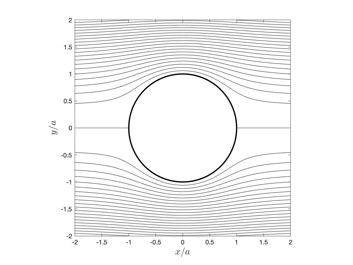
Figure 3: Streamlines of the ideal flow around a sphere

We give here the general relation (III.66) a concrete form for flow around a sphere of radius $a$. The first important ingredient of that relation is the inviscid flow solution ${\bf u}_{\phi}.$ This is well-known (Batchelor (2000), §6.8) to be given in spherical coordinates $(r,\theta,\varphi)$ by the scalar potential

$$\phi=V\left(r+\frac{a^{3}}{2r^{2}}\right)\cos\theta$$ (IV.1)

where, once again, the zenith for measurement of the polar angle $\theta$ is the positive streamwise direction. This implies the potential flow velocity

$$u_{\phi r}=V\left(1-\frac{a^{3}}{r^{3}}\right)\cos\theta,\quad u_{\phi\theta}=-V\left(1+\frac{a^{3}}{2r^{3}}\right)\sin\theta$$ (IV.2)

whose streamlines are plotted in Figure 3 for an axial plane at fixed azimuthal angle $\varphi=0$. It is even more useful to represent this flow by the Stokes stream function (Batchelor (2000), §2.2), given both in spherical coordinates and in cylindrical coordinates $(\sigma,\varphi,x)$ as

$$\psi = \frac{1}{2}Vr^{2}\sin^{2}\theta\left(1-\frac{a^{3}}{r^{3}}\right)$$ (IV.3)

$$= \frac{1}{2}V\sigma^{2}\left[1-\frac{a^{3}}{(\sigma^{2}+x^{2})^{3/2}}\right]$$ (IV.4)

(Batchelor (2000), §6.8) so that

$$u_{\phi x}=\frac{1}{\sigma}\frac{\partial\psi}{\partial\sigma},\quad u_{\phi\sigma}=-\frac{1}{\sigma}\frac{\partial\psi}{\partial x}.$$ (IV.5)

Here we follow the fluid mechanics literature in denoting $\sigma=\sqrt{y^{2}+z^{2}}$ to avoid confusion with mass density $\rho.$ Note that streamlines are uniquely identified by the values of stream function $\psi$ and azimuthal angle $\varphi.$

Although not needed for the Josephson-Anderson relation, it is worth recalling that the pressure $p_{\phi}$ for the ideal Euler solution ${\bf u}_{\phi}$ follows from the Bernoulli equation (III.6) as

$$p_{\phi}=p_{\infty}+\frac{1}{4}{\rm V}^{2}\left(1-\frac{5a^{3}}{4r^{3}}\right)\frac{a^{3}}{r^{3}}+\frac{3}{4}{\rm V}^{2}\left(1-\frac{a^{3}}{4r^{3}}\right)\frac{a^{3}}{r^{3}}\cos(2\theta)$$ (IV.6)

and, in particular, on the surface of the sphere:

$$p_{\phi}(a,\theta)=p_{\infty}-\frac{1}{6}{\rm V}^{2}+\frac{9}{16}{\rm V}^{2}\cos(2\theta).$$ (IV.7)

This ideal pressure distribution is perfectly symmetrical, with maximum value equal to $p_{\infty}+\frac{1}{2}{\rm V}^{2},$ the stagnation pressure, at $\theta=0,\pi$ and minimum $p_{\infty}-\frac{1}{16}{\rm V}^{2}$ at $\theta=\pi/2.$ This symmetry of $p_{\phi}$ around $\theta=\pi/2$ explains, of course, the vanishing drag for ideal flow past a sphere.

We can now use the above results to develop a more concrete expression for the Josephson-Anderson relation (III.66) in the flow around a sphere. First, it is useful to recall that the Stokes stream function is defined for any axisymmetric flow ${\bf u}$ so that $d\psi\,d\varphi={\bf u}{\mbox{\boldmath$\cdot$}}d{\bf A}$ along the streamline labelled by $\psi,$ $\varphi,$ (see Batchelor (2000), §2.2). Thus, the element of mass flux appearing in (III.66) is

$$dJ=\rho{\bf u}_{\phi}{\mbox{\boldmath$\cdot$}}d{\bf A}=\rho\,d\psi\,d\varphi.$$ (IV.8)

It is also straightforward to obtain from (IV.4) an explicit parameterization of the streamlines with fixed $\psi$ in the form $x=\pm x(\sigma;\psi)$ for $\sigma_{\min}(\psi)<\sigma<\sigma_{\max}(\psi)$ and with azimuthal angle $\varphi$ constant independent of $\sigma.$ However, for the qualitative arguments that we make in the next section, the plots of the streamlines in Figure 3 are more useful than these analytical expressions.

We shall furthermore require in the next section a projected version of the vorticity conservation equation (II.5) for the azimuthal vorticity $\omega_{\varphi},$ which we will see is the most crucial component of vorticity for origin of drag. Here we follow a general idea of Huggins Huggins (1994), who observed that one can obtain a balance in any plane for the out-of-plane vorticity $\omega_{n}$ by dotting (II.5) on the right with the unit vector $\hat{{\bf N}}$ normal to the plane. The application of this idea to $\omega_{\varphi}$ involves one subtlety, however: the sets of constant $\varphi$ are half-planes terminating on the $x$-axis, not full planes. Thus, dotting (II.5) with the unit vector $\hat{{\bf N}}=\hat{{\mbox{\boldmath$\varphi$}}}$ for one such half-plane at constant $\varphi$ yields a planar conservation law

$$\partial_{t}\omega_{n}+{\mbox{\boldmath$\nabla$}}{\mbox{\boldmath$\cdot$}}{\mbox{\boldmath$\dot{\j}$}}_{n}=0$$ (IV.9)

in the entire plane normal to $\hat{{\bf N}},$ with

$$\omega_{n}={\mbox{\boldmath$\omega$}}{\mbox{\boldmath$\cdot$}}\hat{{\bf N}},\quad{\mbox{\boldmath$\dot{\j}$}}_{n}={\mbox{\boldmath$\Sigma$}}{\mbox{\boldmath$\cdot$}}\hat{{\bf N}}.$$ (IV.10)

Note that ${\rm j}_{n\,k}=\epsilon_{knl}({\bf u}{\mbox{\boldmath$\times$}}{\mbox{\boldmath$\omega$}}-\nu{\mbox{\boldmath$\nabla$}}{\mbox{\boldmath$\times$}}{\mbox{\boldmath$\omega$}})_{l}$ lies in the plane. However, only the upper part of this plane corresponds to azimuthal angle $\varphi,$ whereas the lower part corresponds instead to the half plane with azimuthal angle $\varphi+\pi$ and whose normal vector is $\hat{{\mbox{\boldmath$\varphi$}}}=-\hat{{\bf N}}.$ Thus, only in the upper half plane does $\omega_{n}=\omega_{\varphi},$ whereas in the lower half-plane $\omega_{n}=-\omega_{\varphi}.$ We shall see that the conservation laws (IV.9), which hold separately for each plane through the $x$-axis, are very useful for elucidating the physics.

IV.2 Physical Consequences

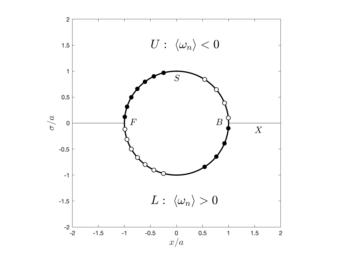
Figure 4: Schematic of azimuthal vorticity generation on the surface of the sphere. Following the convention of Huggins Huggins (1994), we use white circles to denote vorticity out of the plane ($\omega_{n}>0$) and black circles to denote vorticity into the plane ($\omega_{n}<0$). The mean normal (azimuthal) vorticity in the upper half-plane $U$ is negative and the mean normal (anti-azimuthal) vorticity in the lower half-plane $L$ is positive, implying a pole-to-pole asymmetry in the pressure distribution on the surface $S$ of the sphere. The pressure
drop along the surface of the sphere from $F$ to $B$ is exactly compensated by the pressure rise from $B$ to infinity along the direction of the positive streamwise axis $X$.

We shall now exploit the Josephson-Anderson relation (III.66) and its time-averaged form (III.70) in order to develop an exact but qualitative picture of the origin of drag in terms of vortex dynamics. Although our picture has the nature of a “cartoon” which ignores many complex details of the flow in its different regimes (i)-(viii), we argue that it describes the essence of the phenomenon. The concrete predictions that we make should be verifiable empirically in each regime, realized somewhat differently by the specific flow features that are characteristic of that regime which determine the drag quantitatively.

An important general deduction from (III.66) is that vorticity ${\mbox{\boldmath$\omega$}}\parallel{\bf u}_{\phi}$ does not contribute directly to drag, and, furthermore, that vorticity flux in the directions of ${\bf u}_{\phi}$ or $\omega$ do not contribute. As can be seen from Fig.3, ${\bf u}_{\phi}\propto\hat{{\bf x}}$ to a good approximation already at distances about one radius away from the sphere. Thus, we see that, throughout most of the flow, streamwise vorticity $\omega_{x}$ makes no direct contribution to the drag. Although streamwise vorticity appears in the wake, e.g. in the pair of trailing vortices in regime (ii), these features do not contribute anything to (III.66). On the other hand, at the surface of the sphere where all flow vorticity is generated and in its close vicinity, ${\bf u}_{\phi}\propto\hat{{\mbox{\boldmath$\theta$}}}$ so that it is the polar vorticity $\omega_{\theta}$ which does not contribute to drag in that region. Since all of the vorticity on the sphere is parallel to its surface, it follows that the azimuthal vorticity $\omega_{\varphi}$ plays the crucial role and, in particular, its viscous flux $\Sigma_{r\varphi}$ radially outward. This is our first essential conclusion about the origin of drag in the flow past a sphere.

The next implication of (III.66) is that outward flux of negative azimuthal vorticity $\omega_{\varphi}<0$ increases drag, whereas flux of positive azimuthal vorticity $\omega_{\varphi}>0$ in fact decreases drag. Since the mean power consumption by drag can only be positive (see (III.68)), it follows that outward flux of negative azimuthal vorticity must be larger in magnitude. In other words, there must be an asymmetry in sign of the azimuthal vorticity on the sphere, with more area and/or stronger magnitudes where $\omega_{\varphi}<0$ and less areas or magnitudes for $\omega_{\varphi}>0.$ This situation is illustrated by the cartoon in Figure 4. According to Lighthill’s theory Lighthill (1963), the rate of generation of $\omega_{\varphi}$ is exactly $\sigma_{\varphi}=\frac{1}{a}\frac{\partial p}{\partial\theta},$ so that negative azimuthal vorticity is generated by negative or “favorable” pressure gradient, and positive vorticity by positive or “adverse” pressure gradient. We thus conclude that there must be greater area or greater magnitudes of favorable pressure gradient near the front of the sphere than the area or magnitudes of adverse pressure gradient toward the back. This results in a pressure asymmetry unlike that for ideal flow, with the base pressure $p_{B}$ behind the sphere not fully recovering from its drop in the front, thus remaining lower than the stagnation pressure $p_{F}=p_{\infty}+\frac{1}{2}{\rm V}^{2}$ in the front. Along the sphere surface $S$

$$p_{B}-p_{F}=p(a,0)-p(a,\pi)=\int_{\pi}^{0}\frac{\partial p}{\partial\theta}\,d\theta<0.$$ (IV.11)

Of course, these conclusions are all in agreement with common observations but it is now seen how they are required for the generation of drag by vortex dynamics.

The picture in Figure 4 for an axial plane corresponds in three dimensions to generation of azimuthal vortex loops or rings on the surface of the sphere. Those in the front of the sphere have $\omega_{\varphi}<0$ while those toward the rear have mostly $\omega_{\varphi}>0.$ As these rings flow radially outward from the surface, they encircle greater amounts of the potential mass-flux $J,$ with the negative-$\omega_{\varphi}$ rings removing proportionate energy from the potential flow and positive-$\omega_{\varphi}$ rings returning that energy. Since $\omega_{\varphi}<0$ predominates, the net effect is a transfer of kinetic energy from potential to vortical motions, where it is ultimately dissipated by viscosity. In the axisymmetric wake regime (i) this picture is exact, because all vorticity is azimuthal. In higher-$Re$ regimes there will also be some polar vorticity $\omega_{\theta}$ generated on the sphere by azimuthal pressure gradients as $\sigma_{\theta}=-\frac{1}{a}\frac{\partial p}{\partial\varphi},$ but these components and their radial flux from the sphere do not contribute to the drag. See Figure 5 for a rough cartoon of the mechanism. It should be noted that this entire picture developed on the basis of the relation (III.66) is consistent with the direct formula (III.60) for the drag force ${\bf F}$, since the asymmetry in pressure $P$ and the negative azimuthal vorticity $\omega$ on the surface of the sphere result in pressure and viscous forces both opposing the fluid velocity ${\bf V}.$

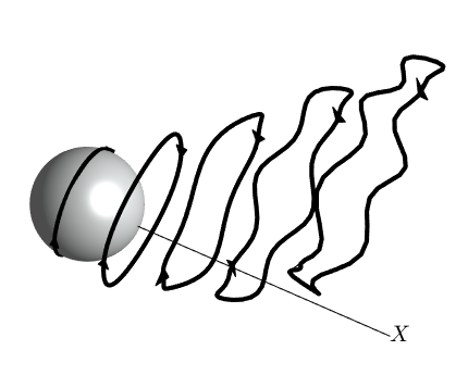
Figure 5: Rough cartoon of the drag mechanism by generation and outward flux of vortex loops with negative azimuthal vorticity. The rings are generated by pressure drop along the surface. As the rings expand outward, they enclose greater mass flux $J$ and subtract proportionate energy from the potential flow. Although the rings initially loop around the streamwise axis $X,$ they drift across in time. This implies a flux of azimuthal vorticity across $X$ and allows the pressure to recover far downstream from its drop around the sphere.

As the vortex loops grow, they enter the region where ${\bf u}_{\phi}\propto\hat{{\bf x}}$ and then azimuthal vorticity $\omega_{\varphi}$ is no longer the only relevant component. Indeed, referring now to the cylindrical coordinate system, axial vorticity $\omega_{\sigma}$ appears in this region through the tilting of azimuthal vorticity by the shear in the wake, e.g. as alternating hairpin vortices observed in the shedding regime (iii). It is easy to check that the flux $\Sigma_{\varphi\sigma}$ due to opposite azimuthal motion of the two legs of growing hairpin vortices, one with $\omega_{\sigma}>0$ and the other with $\omega_{\sigma}<0,$ contributes also to drag through the relation (III.66) in this spatial region, in addition to the flux $\Sigma_{\sigma\varphi}$ of negative azimuthal vorticity axially outward. In fact, these two effects are basically the same because of the anti-symmetry $\Sigma_{\varphi\sigma}=-\Sigma_{\sigma\varphi}$ and both correspond to growth of the tilted vortex rings, which encompass an increasing amount of mass flux $J$ and gain a proportionate amount of energy from the potential flow. This is the essential mechanism of drag in terms of vortex dynamics for the flow around a sphere as already illustrated in Figure 5.

Conservation of azimuthal vorticity has one very important additional implication for this process. We showed at the end of section III.6 that $\Delta h^{\prime}=0$ along each streamline of the potential flow. Since now $\dot{\phi}=0,$ $h^{\prime}=h$ and $h(\ell=\pm\infty)=h_{\infty}=p_{\infty}+\frac{1}{2}{\rm V}^{2}$ at each limit of the streamline. Notice that this value is the same as the stagnation pressure at the front of the sphere $h_{F}=p_{F}=p_{\infty}+\frac{1}{2}{\rm V}^{2}$ and also that $h_{B}=p_{B}$ at the base point behind the sphere, since the fluid velocity vanishes everywhere on the surface. We thus see that the decrease of $h$ on the surface $S$ of the sphere

$$\int_{\pi}^{0}\frac{\partial h}{\partial\theta}(a,\theta)\,d\theta=h_{B}-h_{F}<0$$ (IV.12)

is exactly equal and opposite to the increase of $h$ along the streamwise axis $X$ from the base of the sphere to infinity:

$$\int_{a}^{\infty}\frac{\partial h}{\partial x}(0,x)\,dx=h_{\infty}-h_{B}>0$$ (IV.13)

See Figure 4. Since $\langle\Sigma_{r\varphi}\rangle=\frac{1}{a}\frac{\partial\langle h\rangle}{\partial\theta}$ on $S$ and $\langle\Sigma_{\sigma\varphi}\rangle=\frac{\partial\langle h\rangle}{\partial x}$ on $X$, it follows that, on average, the net negative azimuthal vorticity generated on the surface of the sphere is exactly cancelled by flux of opposite-signed vorticity across the $x$-axis. This fact was previously noted by Brown & Roshko Brown and Roshko (2012) for flow around a cylinder and by Terrington et al. Terrington et al. (2021) for flow around a sphere. This exact balance is what permits a steady state to exist with a mean negative value $\langle\omega_{\varphi}\rangle<0$ in the axial half-planes for each fixed value of $\varphi.$ The precise origin of the flux across the $x$-axis is still debated, but it is most likely due to lateral motion of shed vortex rings, which initially loop around the $x$-axis but drift across the $x$-axis to become unlinked from it as they advect downstream. See Figure 5. Although this is a “cartoon picture” assuming simple closed vortex rings, it presumably has an exact counterpart in the actual vortex motions, because solenoidality requires a pairing of the points with $\omega_{\varphi}<0$ on opposite sides of the $x$-axis and viscous or turbulent diffusion will tend to mix those points from one side to the other.

In this section we have attempted to give a clear and intuitive description of the origin of drag in terms of a schematic picture of the vortex motions. Although qualitative, this picture makes specific predictions in terms of the signs of the vorticity components $\omega_{j}$ and their fluxes $\Sigma_{ij},$ which can be checked empirically by measuring these quantities in numerical simulation or experiment and evaluating their contribution to the drag through the relation (III.66). We note that the numerical study Terrington et al. (2021) has already used Huggins’ vorticity flux (II.3) to illuminate other aspects of the vortex dynamics in the wake behind a sphere, such as tilting of the azimuthal vorticity in the streamwise direction

IV.3 Superfluid Comparisons

The cartoon picture that we presented in the previous section in order to interpret the exact Josphson-Anderson relation (III.66) should be more literally correct for a superfluid, where vorticity is quantized and vortex lines are discrete objects whose motion is objectively defined. In fact, the most fundamental differences between our theoretical results and those for superfluids arise not from the differences between classical and quantum fluids, but instead from the differences between incompressible and compressible. In superfluids there are generally substantial compressibility effects, due to emission of phonons that propagate at the finite speed of sound. Of course, the Josephson-Anderson relation arose in the study of superfluids and its application there to understanding drag and critical velocities is well-established. It is therefore worth reviewing briefly the existing literature in order to point out both the similarities and the differences with classical incompressible fluids.

The pioneer work concerning drag acting on bodies moving through a superfluid is that of Frisch et al. Frisch et al. (1992), who adopted the zero-temperature Gross-Pitaevskii model to study numerically the motion of a disk at velocity ${\rm V}$ through a 2D superfluid. We remark that it is straightforward to extend our own analysis for incompressible classical fluids to 2D. Already showing the important effects of compressibility, the authors of Frisch et al. (1992) identified the critical velocity ${\rm V}_{c}$ for appearance of drag to be that for which the local velocity $u$ on the surface of the disk exceeds the sound speed $c_{s}.$ At this velocity ${\rm V}_{c}\doteq 0.44\,c_{s}$, quantized vortices are nucleated and emitted as a wake behind the disk. Although compressibility plays a crucial role in their generation, the vortices themselves are incompressible excitations in the superfluid. The picture proposed in Frisch et al. (1992) has been further developed in many subsequent works on this same problem Jackson et al. (1998); Winiecki et al. (1999, 2000); Winiecki (2001); Huepe and Brachet (2000); Nore et al. (2000); Sasaki et al. (2010). In particular, we note that the generation of the vortices has been verified to occur by the $2\pi$-phase slip mechanism Jackson et al. (1998) and their shedding occurs with the Josephson frequency corresponding to the difference in the generalized chemical potential $\mu_{T}=gn+\frac{1}{2}mu^{2}$ that develops between the exterior flow and the wake behind the disk with low density $n$ and low speed $u$ Winiecki et al. (1999). Thus, at least for ${\rm V}<c_{s},$ there is great similarity with the theory that we have developed for classical, incompressible fluids. Of course, for supersonic motions with ${\rm V}>c_{s},$ new compressible effects can be observed in superfluids, such as drag by phonon radiation and standing bow waves in front of the disk Winiecki et al. (2000); Winiecki (2001), which have no parallel in the incompressible theory developed here.

Studies of superfluid drag have since been extended to 3D, with the superfluid modeled again by Gross-Pitaevskii and the moving object by a suitable time-dependent potential Winiecki and Adams (2000); Stagg et al. (2014). The object was taken in Winiecki and Adams (2000) to be spherical and subject to constant force ${\bf F},$ whereas Stagg et al. (2014) considered more general ellipsoidal bodies and moving at constant velocity ${\bf V}.$ The picture emerging from these 3D simulation studies is even more strikingly similar to the one that we have derived for classical fluids. In both studies, quantized vortex rings are excited at the surface of the object when it reaches the critical speed ${\rm V}_{c},$ with the vorticity oriented in the negative azimuthal direction (according to our coordinate conventions). In the case of the body moving at constant speed studied in Stagg et al. (2014), the ring vortices are shed into the wake where they grow, extracting energy from the potential flow, and also drift cross-stream so that the asymmetry in the vortex polarity is relaxed far downstream. The observed simulation results are very close to our sketch in Figure 5. The case with constant applied force ${\bf F}$ studied in Winiecki and Adams (2000) shows a bit more complex behavior, because the body decelerates when the vortex ring is emitted. At lower forcing, the quantized vortex ring reattaches to the spherical body and remains pinned there as an arch, legs perpendicular to the surface, even as it continues to grow and expand outward. This regime has no strict classical analogue, although it distantly resembles the reattachment of the separating laminar boundary layer observed in the “drag crisis” of the classical regime (vi). At higher forcing, however, the vortex rings completely detach and are shed in the wake, again very similar to our Figure 5.

Somewhat ironically, the detailed Josephson-Anderson relation was derived by Huggins Huggins (1970a) assuming flow incompressibility, and we are aware of no full extension to the Gross-Pitaevskii model of a superfluid. The original Josephson-Anderson phase relation (I.1) is, of course, directly embodied in the Gross-Pitaevskii equation (with an additional “quantum pressure” term), but this implies no direct connection of vortex motion with energy dissipation. Thus, based on our results in the present paper, we currently have a better understanding for a classical incompressible fluid how energy dissipation is associated to vorticity flux than we do for quantum superfluids, where the Josephson-Anderson relation originated!

V Why is It Important?

To briefly summarize our results in this paper, we have derived the detailed Josephson-Anderson relation (III.66) for incompressible fluid flow around a finite solid body, relating drag and energy dissipation to vorticity flux and implying a time-averaged version (III.68) valid for the local steady-states of the fluid wake. We have furthermore discussed in detail the origins of drag in terms of vortex motion for the concrete example of flow past a sphere, obtaining numerous predictions that can be checked empirically. But why are these results important?

We believe first of all that the Josephson-Anderson relation is important because of the theoretical unity that it brings to our understanding of drag for both quantum and classical fluid systems, across all Reynolds number ranges of the latter. The relation clearly identifies what is essential for drag in the vortex dynamics and statistics, bypassing all details of secondary importance. In the classical case, these “details” include fascinating phenomena such as boundary-layer separation, formation of streamwise vortices by tilting, transition to turbulence first in the wake and then in the boundary-layer, etc. All such “details” are, of course, crucial in order to determine the drag quantitatively, but only insofar as they modify the primary process: flux of vorticity across the potential mass flux. The precise vortex dynamics and statistics which contribute to the Josephson-Anderson relation must be explained in any quantitative theory of drag.

The relation (III.66) furthermore sheds new insight on the D’Alembert paradox d’Alembert (1749); Grimberg et al. (2008). We should emphasize that, in our opinion, the paradox in its original form had its solution in the realization by Saint-Venant of the importance of even a very small viscosity Saint-Venant (1846), as further elaborated by Prandtl Prandtl (1904) and others Stewartson (1981). However, the paradox has recently arisen in a new guise, because of two apparently conflicting facts, one empirical and the other mathematical. The empirical fact from laboratory observations is that the dimensionless drag coefficient $C_{D}(Re)$ for flow around a finite object such as a sphere apparently tends to a non-zero constant value as $Re\to\infty$ Achenbach (1972).
The mathematical fact is that, under very modest assumptions, the viscous Navier-Stokes solution must tend in the limit $Re\to\infty$ (along a suitable subsequence) to a weak solution of the incompressible Euler equations Drivas and Nguyen (2019). The “paradox” is then how the limiting weak Euler solution can produce a non-vanishing drag.

This puzzle is obviously connected with the Onsager theory of turbulence in terms of dissipative weak solutions of the Euler equations Onsager (1949b); Eyink and Sreenivasan (2006); Eyink (2018). In fact, our results in this paper open up the possibility of a novel analysis that directly relates the D’Alembert paradox with Onsager’s theory. One crucial observation is that the new potential-vortical formulation (III.18) of incompressible Navier-Stokes is a local conservation equation for $\rho{\bf u}_{\omega},$ the density of “vortex momentum”, and it thus has a weak interpretation. We may therefore apply in this formulation the recent techniques to derive Onsager’s theory for wall-bounded flows Bardos and Titi (2018); Drivas and Nguyen (2018); Bardos et al. (2019); Chen et al. (2020), obtaining necessary conditions for non-vanishing drag and dissipation in the infinite Reynolds-number limit. The relevant limiting Euler solutions must obviously describe rotational flow very distinct from the smooth potential-flow solution. The local energy balances (III.25), (III.28) make sense also in a weak interpretation and, in the infinite-$Re$ limit, the viscous dissipation appearing in (III.25) will yield a “dissipative anomaly” like that appearing in the work of Duchon & Robert for periodic domains Duchon and Robert (2000). However, a priori the energy transfer term in the two equations (III.25), (III.28) may have no limit because the pointwise product ${\bf u}_{\omega}{\mbox{\boldmath$\times$}}\omega$ has no clear meaning when ${\bf u}_{\omega}$ and $\omega$ for the limiting Euler solution are merely distributions. Fortunately, this term can be rewritten as a space-gradient using the familiar vector calculus identity

$${\bf u}_{\omega}{\mbox{\boldmath$\times$}}{\mbox{\boldmath$\omega$}}=-{\mbox{\boldmath$\nabla$}}{\mbox{\boldmath$\cdot$}}\left[{\bf u}_{\omega}{\bf u}_{\omega}-\frac{1}{2}|{\bf u}_{\omega}|^{2}{\bf I}\right]$$ (V.1)

and this is a well-defined distribution even if ${\bf u}_{\omega}$ is only square-integrable. Because the potential-flow solution ${\bf u}_{\phi}$ is smooth, this observation allows us to rewrite the transfer term in the Josephson-Anderson relation (III.66) as

$$\int_{\Omega}{\bf u}_{\phi}{\mbox{\boldmath$\cdot$}}({\bf u}_{\omega}{\mbox{\boldmath$\times$}}{\mbox{\boldmath$\omega$}})\,dV=\int_{\Omega}{\mbox{\boldmath$\nabla$}}{\bf u}_{\phi}{\mbox{\boldmath$:$}}{\bf u}_{\omega}{\bf u}_{\omega}\,dV$$ (V.2)

and, in this form, the relation can be valid even for the limiting weak solutions of Euler equations Eyink et al. (2021). It is very natural that drag for the limiting Euler solution should be connected with vorticity flux since, as emphasized by Morton Morton (1984), generation of vorticity at the wall by tangential pressure-gradients is a purely inviscid process.

Of more immediate importance for practical applications is the new insight that the Josephson-Anderson relation (III.66) provides on techniques for drag reduction. As discussed previously Huggins (1994); Eyink (2008), a “drag problem” occurs not only in turbulent flow at high Reynolds number but also in high-temperature superconductors because, above a critical electric current, quantized magnetic flux-lines are nucleated which migrate cross-current and create a voltage drop and effective resistance Josephson (1965); Bishop et al. (1993). The technological solution that has been found is to introduce some sort of disorder to pin the quantized lines so that they are not free to cross the current, permitting resistance-less conduction up to higher values of electric current. It might be thought that vortices cannot be so easily “pinned” in a classical fluid with smoothly distributed vorticity, but, in fact, the Josephson-Anderson relation (III.66) tells us that any mechanism which reduces drag must somehow decrease vorticity flux across the potential mass current! This includes mechanisms such as drag reduction by polymer additives or the Toms effect, Toms (1948); White and Mungal (2008), whose efficacy is well-documented but whose detailed physical explanation is still debated. We believe that empirical investigation of the vorticity flux will provide new clues into the underlying mechanism.

Granted that the detailed Josephson-Anderson relation (III.66) has important implications, it then becomes interesting to explore the full range of its validity. Although bodies of finite extent are most realistic, it should be illuminating to generalize the relation to more idealized geometries such as flow past cylinders and semi-infinite plates. Validity of the relation for compressible flow would greatly widen the range of applications and we believe that this could be possible, especially for barotropic models where smooth Euler solutions satisfy a Kelvin circulation theorem and potential flow conditions are preserved in time (including the Gross-Pitaevskii model). Finally, there should be a connection with stochastic Lagrangian representation of the vorticity dynamics Constantin and Iyer (2008, 2011); Eyink et al. (2020a, b), which gives a more precise meaning to the “motion” of vortex lines in a classical fluid. This approach has recently been generalized to solve the Helmholtz equation with the Lighthill vorticity source as Neumann boundary conditions Eyink and Peng (2021); Wang et al. (2021), but it is not yet clear how to relate the stochastic Lagrangian trajectories to the Huggins vorticity flux tensor in the flow interior. These stochastic representations are an exact mathematical approach to realize Huggins’ suggestion Huggins (1971) of a probability interpretation of the vorticity field.

Appendix A Derivation of Huggins’ Relation

For completeness, we reproduce here the derivation of the detailed Josephson-Anderson relation for the channel-flow geometry, originally obtained by Huggins. The starting point is the Bernoulli equation for the scalar potential of the ideal flow:

$$\dot{\phi}+\frac{1}{2}|{\bf u}_{\phi}|^{2}+p_{\phi}+U=0.$$ (A.1)

Its space-gradient is the Euler equation for ${\bf u}_{\phi}={\mbox{\boldmath$\nabla$}}\phi,$ which, subtracted from the Navier-Stokes equation (II.1), yields the equation of motion for ${\bf u}_{\omega}:={\bf u}-{\bf u}_{\phi}:$

$$\partial_{t}{\bf u}_{\omega}={\bf u}{\mbox{\boldmath$\times$}}{\mbox{\boldmath$\omega$}}-\nu{\mbox{\boldmath$\nabla$}}{\mbox{\boldmath$\times$}}{\mbox{\boldmath$\omega$}}-{\bf g}-{\mbox{\boldmath$\nabla$}}\left(p_{\omega}+\frac{1}{2}|{\bf u}_{\omega}|^{2}+{\bf u}_{\omega}{\mbox{\boldmath$\cdot$}}{\bf u}_{\phi}\right),$$ (A.2)

with the boundary conditions

$$\left.{\bf u}_{\omega}\right|_{S_{in}}={\mbox{\boldmath$0$}},\quad\left.{\bf u}_{\omega}\right|_{S_{out}}={\mbox{\boldmath$0$}},\quad\left.{\bf u}_{\omega}\right|_{S_{w}}={\mbox{\boldmath$0$}}.$$ (A.3)

Dotting (A.2) with ${\bf u}_{\omega}$ and integrating over the channel domain $\Omega$ immediately yields

$$\frac{dE_{\omega}}{dt}={\mathcal{T}}-\int_{\Omega}[\eta|{\mbox{\boldmath$\omega$}}|^{2}+\rho{\bf u}{\mbox{\boldmath$\cdot$}}{\bf g}]\,dV$$ (A.4)

which is (II.11) in the main text. On the other hand, the total kinetic energy $E(t)=(1/2)\int\rho|{\bf u}|^{2}\,dV$ satisfies

$$\frac{dE}{dt}=\int dJ(h_{in}-h_{out})-\int_{\Omega}[\eta|{\mbox{\boldmath$\omega$}}|^{2}+\rho{\bf u}{\mbox{\boldmath$\cdot$}}{\bf g}]\,dV$$ (A.5)

and since $E=E_{\phi}+E_{\omega}$ by the Kelvin minimum energy theorem, we obtain

$$\frac{dE_{\phi}}{dt}=\int dJ(h_{in}-h_{out})-{\mathcal{T}}$$ (A.6)

which is (II.10) in the main text. Finally,

$$\frac{dE_{\phi}}{dt} = \int_{\Omega}\rho{\bf u}_{\phi}{\mbox{\boldmath$\cdot$}}\dot{{\bf u}}_{\phi}\,dV$$ (A.7)

$$= \int_{\Omega}\rho{\mbox{\boldmath$\nabla$}}{\mbox{\boldmath$\cdot$}}(\dot{\phi}{\bf u}_{\phi})\,dV=\int dJ(\dot{\phi}_{out}-\dot{\phi}_{in})$$ (A.8)

by using the divergence theorem and $dJ=\rho{\bf u}_{\phi}{\mbox{\boldmath$\cdot$}}d{\bf A}.$ Combining (A.6) and (A.8) yields

$${\mathcal{T}}=\int dJ(h_{in}^{\prime}-h_{out}^{\prime})$$ (A.9)

which is the “detailed Josephson relation” (II.16) first derived by Huggins.

Appendix B Vortex Momentum and Impulse

We give here another derivation of (III.49), different from that of Cantwell (1986). Using the identity

$${\bf x}{\mbox{\boldmath$\times$}}{\mbox{\boldmath$\omega$}}=x_{i}{\mbox{\boldmath$\nabla$}}u_{\omega i}-({\bf x}{\mbox{\boldmath$\cdot$}}{\mbox{\boldmath$\nabla$}}){\bf u}_{\omega}$$ (B.1)

we find after integration by parts that

$$\int_{\Omega}{\bf x}{\mbox{\boldmath$\times$}}{\mbox{\boldmath$\omega$}}\,dV=\int_{\Omega}(-1+3){\bf u}_{\omega}\,dV$$ (B.2)

$$-\int_{\partial B}{\bf x}{\mbox{\boldmath$\times$}}(\hat{{\bf n}}{\mbox{\boldmath$\times$}}{\bf u}_{\omega})\,dA+\lim_{R\to\infty}\int_{S_{R}}{\bf x}{\mbox{\boldmath$\times$}}(\hat{{\bf r}}{\mbox{\boldmath$\times$}}{\bf u}_{\omega})\,dA$$ (B.3)

or from the definition of ${\bf I}_{\omega}$

$$2{\bf I}_{\omega}=2\int_{\Omega}{\bf u}_{\omega}\,dV+\lim_{R\to\infty}\int_{S_{R}}{\bf x}{\mbox{\boldmath$\times$}}(\hat{{\bf r}}{\mbox{\boldmath$\times$}}{\bf u}_{\omega})\,dA$$ (B.5)

Using the asymptotic far-field expansion of ${\bf u}_{\omega}$

$$\lim_{R\to\infty}\int_{S_{R}}{\bf x}{\mbox{\boldmath$\times$}}(\hat{{\bf r}}{\mbox{\boldmath$\times$}}{\bf u}_{\omega})\,dA\ =\ \lim_{R\to\infty}\int_{S_{R}}R\hat{{\bf r}}{\mbox{\boldmath$\times$}}\frac{\hat{{\bf r}}{\mbox{\boldmath$\times$}}(-{\bf I}_{\omega})}{4\pi R^{3}}\ R^{2}\,d\Omega$$ (B.6)

$$\hskip 50.0pt=\frac{1}{4\pi}\int({\bf I}_{\omega}-({\bf I}_{\omega}{\mbox{\boldmath$\cdot$}}\hat{{\bf r}})\hat{{\bf r}})\ d\Omega\ =\ \frac{2}{3}{\bf I}_{\omega}$$ (B.7)

Thus, we finally obtain

$$\int_{\Omega}{\bf u}_{\omega}\,dV=\frac{2}{3}{\bf I}_{\omega}.$$ (B.8)

References

- Josephson (1962) Brian D Josephson, “Possible new effects in superconductive tunnelling,” Physics letters 1, 251–253 (1962).
- Anderson (1966) Philip W Anderson, “Considerations on the flow of superfluid helium,” Reviews of Modern Physics 38, 298 (1966).
- Packard (1998) Richard E Packard, “The role of the Josephson-Anderson equation in superfluid helium,” Reviews of Modern Physics 70, 641 (1998).
- Varoquaux (2015) Eric Varoquaux, “Anderson’s considerations on the flow of superfluid helium: Some offshoots,” Reviews of Modern Physics 87, 803 (2015).
- Onsager (1949a) L. Onsager, “Discussion remark on ‘The two fluid model for Helium II’, by C. J. Gorter,” Nuovo Cimento Suppl. 6, 249–251 (1949a).
- Feynman (1955) Richard P Feynman, “Application of quantum mechanics to liquid helium,” in Progress in low temperature physics, Vol. 1 (Elsevier, 1955) Chap. II, pp. 17–53.
- Josephson (1965) BD Josephson, “Potential differences in the mixed state of type II superconductors,” Phys. Lett. 16, 242–243 (1965).
- Huggins (1970a) Elisha R Huggins, “Energy-dissipation theorem and detailed Josephson equation for ideal incompressible fluids,” Physical Review A 1, 332 (1970a).
- Zimmermann (1993) W Zimmermann, “Energy transfer and phase slip by quantum vortex motion in superfluid He,” Journal of Low Temperature Physics 93, 1003–1018 (1993).
- Greiter (2005) Martin Greiter, “Is electromagnetic gauge invariance spontaneously violated in superconductors?” Annals of Physics 319, 217–249 (2005).
- Bishop et al. (1993) David J Bishop, Peter L Gammel, and David A Huse, “Resistance in high-temperature superconductors,” Scientific American 268, 48–55 (1993).
- Note (1) The author had a conversation with Anderson about this during a sabbatical at Princeton in 2017 and Anderson still maintained the opinion at that time that the relation was of special importance in superfluids where vortices are quantized and was not obviously useful in classical hydrodynamics.
- Huggins (1994) Elisha R Huggins, “Vortex currents in turbulent superfluid and classical fluid channel flow, the Magnus effect, and Goldstone boson fields,” Journal of low temperature physics 96, 317–346 (1994).
- Note (2) Elisha Huggins was a PhD student of Richard Feynman, from whom he may have inherited his interest in classical fluid turbulence.
- Taylor (1932) Geoffrey Ingram Taylor, “The transport of vorticity and heat through fluids in turbulent motion,” Proceedings of the Royal Society of London. Series A, Containing Papers of a Mathematical and Physical Character 135, 685–702 (1932).
- Lighthill (1963) M. J. Lighthill, “Introduction: Boundary layer theory,” in Laminar Boundary Theory, edited by L. Rosenhead (Oxford University Press, Oxford, 1963) pp. 46–113.
- Huggins (1970b) Elisha R Huggins, “Exact Magnus-force formula for three-dimensional fluid-core vortices,” Physical Review A 1, 327 (1970b).
- Huggins (1971) Elisha R Huggins, “Dynamical theory and probability interpretation of the vorticity field,” Physical Review Letters 26, 1291 (1971).
- Eyink (2008) Gregory L Eyink, “Turbulent flow in pipes and channels as cross-stream ‘inverse cascades’ of vorticity,” Physics of Fluids 20, 125101 (2008).
- Kelvin (1882) Lord Kelvin, “On vis-viva of a liquid in motion, Cambridge and Dublin Math. J. (1849),” in Mathematical and Physical Papers: Collected from Different Scientific Periodicals from May, 1841, to the Present Time, Vol. I (C. J. Clay & Sons, Cambridge University Press, 1882).
- d’Alembert (1749) Jean le Rond d’Alembert, “Theoria resistentiae quam patitur corpus in fluido motum, ex principiis omnino novis et simplissimis deducta, habita ratione tum velocitatis, figurae, et massae corporis moti, tum densitatis compressionis partium fluidi,” manuscript at Berlin-Brandenburgische Akademie der Wissenschaften, Akademie-Archiv call number: I-M478 (1749).
- d’Alembert (1768) Jean le Rond d’Alembert, “Paradoxe proposé aux géomètres sur la résistance des fluides,” in: Opuscules mathématiques, vol. 5 (Paris), Memoir XXXIV, Section I, 132–138 (1768).
- Grimberg et al. (2008) Gérard Grimberg, Walter Pauls, and Uriel Frisch, “Genesis of d’Alembert’s paradox and analytical elaboration of the drag problem,” Physica D: Nonlinear Phenomena 237, 1878–1886 (2008).
- Frisch et al. (1992) Thomas Frisch, Yves Pomeau, and Sergio Rica, “Transition to dissipation in a model of superflow,” Physical review letters 69, 1644 (1992).
- Jackson et al. (1998) B Jackson, JF McCann, and CS Adams, “Vortex formation in dilute inhomogeneous Bose-Einstein condensates,” Physical Review Letters 80, 3903 (1998).
- Winiecki et al. (1999) T Winiecki, JF McCann, and CS Adams, “Pressure drag in linear and nonlinear quantum fluids,” Physical review letters 82, 5186 (1999).
- Winiecki et al. (2000) T Winiecki, B Jackson, JF McCann, and CS Adams, “Vortex shedding and drag in dilute Bose-Einstein condensates,” Journal of Physics B: Atomic, Molecular and Optical Physics 33, 4069 (2000).
- Winiecki and Adams (2000) T Winiecki and CS Adams, “Motion of an object through a quantum fluid,” EPL (Europhysics Letters) 52, 257 (2000).
- Winiecki (2001) Thomas Winiecki, Numerical studies of superfluids and superconductors, Ph.D. thesis, Durham University (2001).
- Huepe and Brachet (2000) Cristián Huepe and Marc-Etienne Brachet, “Scaling laws for vortical nucleation solutions in a model of superflow,” Physica D: Nonlinear Phenomena 140, 126–140 (2000).
- Nore et al. (2000) C Nore, C Huepe, and ME Brachet, “Subcritical dissipation in three-dimensional superflows,” Physical review letters 84, 2191 (2000).
- Sasaki et al. (2010) Kazuki Sasaki, Naoya Suzuki, and Hiroki Saito, “Bénard–von Kármán vortex street in a Bose-Einstein condensate,” Physical review letters 104, 150404 (2010).
- Stagg et al. (2014) GW Stagg, NG Parker, and CF Barenghi, “Quantum analogues of classical wakes in Bose–Einstein condensates,” Journal of Physics B: Atomic, Molecular and Optical Physics 47, 095304 (2014).
- Stagg et al. (2015) GW Stagg, AJ Allen, NG Parker, and CF Barenghi, “Generation and decay of two-dimensional quantum turbulence in a trapped Bose-Einstein condensate,” Physical Review A 91, 013612 (2015).
- Musser et al. (2019) Seth Musser, Davide Proment, Miguel Onorato, and William TM Irvine, “Starting flow past an airfoil and its acquired lift in a superfluid,” Physical review letters 123, 154502 (2019).
- Onsager (1949b) Lars Onsager, “Statistical hydrodynamics,” Nuovo Cim. Suppl. 6, 279–287 (1949b).
- Eyink and Sreenivasan (2006) Gregory L Eyink and Katepalli R Sreenivasan, “Onsager and the theory of hydrodynamic turbulence,” Rev Mod Phys 78, 87 (2006).
- Eyink (2018) Gregory L Eyink, “Review of the Onsager ‘ideal turbulence’ theory,” arXiv preprint arXiv:1803.02223 (2018).
- Lamb (1945) H. Lamb, Hydrodynamics, Dover Books on Physics (Dover publications, 1945).
- Batchelor (2000) G. K. Batchelor, An Introduction to Fluid Dynamics, Cambridge Mathematical Library (Cambridge University Press, 2000).
- Wu et al. (2007) J.Z. Wu, H. Ma, and M.D. Zhou, Vorticity and Vortex Dynamics, Lecture notes in mathematics (Springer Berlin Heidelberg, 2007).
- Lyman (1990) F. A. Lyman, “Vorticity production at a solid boundary,” Appl. Mech. Rev 43, 157–158 (1990).
- Panton (1984) R.L. Panton, Incompressible Flow (John Wiley & Sons Australia, Limited, 1984).
- Wu and Wu (1993) Jie-Zhi Wu and Jain-Ming Wu, “Interactions between a solid surface and a viscous compressible flow field,” Journal of Fluid Mechanics 254, 183–211 (1993).
- Wu and Wu (1996) JZ Wu and JM Wu, “Vorticity dynamics on boundaries,” Advances in applied mechanics 32, 119–275 (1996).
- Wu and Wu (1998) JZ Wu and JM Wu, “Boundary vorticity dynamics since Lighthill’s 1963 article: review and development,” Theoretical and computational fluid dynamics 10, 459–474 (1998).
- Morton (1984) B. R. Morton, “The generation and decay of vorticity,” Geophysical & Astrophysical Fluid Dynamics 28, 277–308 (1984).
- Kustepeli (2016) Alp Kustepeli, “On the Helmholtz theorem and its generalization for multi-layers,” Electromagnetics 36, 135–148 (2016).
- Vladimirov (1977) V. A. Vladimirov, “Vortical momentum of flows of an incompressible liquid [in Russian],” PMTF Zhurnal Prikladnoi Mekhaniki i Tekhnicheskoi Fiziki 18, 72–77 (1977), English transl, Journal of Applied Mechanics and Technical Physics, 18 (6), 791–794 (1978).
- Payne (1956) Ronald Bruce Payne, “A numerical method for calculating the starting and perturbation of a two-dimensional jet at low Reynolds number,” Aeronautical Research Council, Reports and Memoranda, No. 3047 , 1–50 (1956).
- Payne (1958) R. B. Payne, “Calculations of unsteady viscous flow past a circular cylinder,” Journal of Fluid Mechanics 4, 81–86 (1958).
- Ploumhans et al. (2002) Paul Ploumhans, GS Winckelmans, John K Salmon, Anthony Leonard, and MS Warren, “Vortex methods for direct numerical simulation of three-dimensional bluff body flows: application to the sphere at Re= 300, 500, and 1000,” Journal of Computational Physics 178, 427–463 (2002).
- Branlard (2017) Emmanuel Branlard, “The different aspects of vortex methods,” in Wind Turbine Aerodynamics and Vorticity-Based Methods, Research Topics in Wind Energy, Vol. 7 (Springer, 2017) Chap. 41, pp. 493–543.
- Schwarz (1985) KW Schwarz, “Three-dimensional vortex dynamics in superfluid He: Line-line and line-boundary interactions,” Physical Review B 31, 5782 (1985).
- Föppl (1897) A. Föppl, Die Geometrie der Wirbelfelder (Teubner, Leipzig, 1897).
- Hirsch (2012) M.W. Hirsch, Differential Topology, Graduate Texts in Mathematics (Springer New York, 2012).
- Federer (2014) H. Federer, Geometric Measure Theory, Classics in Mathematics (Springer Berlin Heidelberg, 2014).
- Cantwell (1986) Brian J Cantwell, “Viscous starting jets,” Journal of Fluid Mechanics 173, 159–189 (1986).
- Schwarz (1975) KW Schwarz, “Onset of phase slip in superflow through channels,” Physical Review B 12, 3658 (1975).
- Note (3) Note that Schwarz (1975); Varoquaux (2015) and the superfluid community in general use the notation for the vortex impulse !
- Note (4) Notice that, until this point, none of our analysis requires that the velocity at infinity must be constant in time, and so applies to more general cases of a body linearly accelerating through a fluid, but without body rotation. The Bernoulli equation (III.6\@@italiccorr) simply requires a new term on the righthand side to obtain the Euler equation in the non-inertial body-frame. Body rotation, on the other hand, leads to new effects that are beyond the scope of the present paper.
- Note (5) It is important to note all of the spatial integrals over are absolutely convergent, because of the decay laws and asymptotically at large-. Thus, the integrands both in the detailed Josephson-Anderson relation (III.66\@@italiccorr) and in the viscous dissipation in (III.63\@@italiccorr) are rather well-localized and the integrals can be calculated accurately in a possibly large, but finite-volume region of space.
- Note (6) Note that the two integrands in the second line of (III.73\@@italiccorr) are separately only conditionally convergent, but their combination, which equals the integrand in the first line, is absolutely convergent.
- Tiwari et al. (2020) Shashank S Tiwari, Eshita Pal, Shivkumar Bale, Nitin Minocha, Ashwin W Patwardhan, Krishnaswamy Nandakumar, and Jyeshtharaj B Joshi, “Flow past a single stationary sphere, 2. Regime mapping and effect of external disturbances,” Powder Technology 365, 215–243 (2020).
- Brown and Roshko (2012) Garry L Brown and Anatol Roshko, “Turbulent shear layers and wakes,” Journal of Turbulence , N51 (2012).
- Terrington et al. (2021) S. J. Terrington, K. Hourigan, and M. C. Thompson, “The generation and diffusion of vorticity in three-dimensional flows: Lyman’s flux,” Journal of Fluid Mechanics 915, A106 (2021).
- Note (7) Note that the authors of Terrington et al. (2021) refer to Huggins’ flux in (II.3\@@italiccorr), as “Lyman-Huggins flux”, citing also Lyman (1990). This double attribution is not really proper, in our opinion, since Lyman considered vorticity generated only at the boundary, whereas it was Huggins who first considered this flux in the interior of the flow.
- Saint-Venant (1846) A. Saint-Venant, “Résistance des fluides: considérations historiques, physiques et pratiques relatives au problème de l’action dynamique muteulle d’un fluide a d’un solide, dans l’état de permanence supposé acquis par leurs mouvements,” Academie des Science, Mémoires 44, 1–280 (1846).
- Prandtl (1904) L Prandtl, “Über Flüssigkeitsbewegung mit kleiner Reibung,” Verhandlungen des dritten internationalen Mathematiker-Kongresses in Heidelberg , 484–491 (1904), English transl., “On motion of fluids with very little viscosity,” Third International Congress of Mathematics, Heidelberg, https://ntrs.nasa.gov/api/citations/19930090813/downloads/19930090813.pdf.
- Stewartson (1981) Keith Stewartson, “D’Alembert’s paradox,” SIAM review 23, 308–343 (1981).
- Achenbach (1972) Elmar Achenbach, “Experiments on the flow past spheres at very high Reynolds numbers,” Journal of Fluid Mechanics 54, 565–575 (1972).
- Drivas and Nguyen (2019) Theodore D Drivas and Huy Q Nguyen, “Remarks on the emergence of weak Euler solutions in the vanishing viscosity limit,” Journal of Nonlinear Science 29, 709–721 (2019).
- Bardos and Titi (2018) Claude Bardos and Edriss S Titi, “Onsager’s conjecture for the incompressible Euler equations in bounded domains,” Archive for Rational Mechanics and Analysis 228, 197–207 (2018).
- Drivas and Nguyen (2018) Theodore D Drivas and Huy Q Nguyen, “Onsager’s conjecture and anomalous dissipation on domains with boundary,” SIAM Journal on Mathematical Analysis 50, 4785–4811 (2018).
- Bardos et al. (2019) Claude Bardos, Edriss S Titi, and Emil Wiedemann, “Onsager’s conjecture with physical boundaries and an application to the vanishing viscosity limit,” Communications in Mathematical Physics 370, 291–310 (2019).
- Chen et al. (2020) Robin Ming Chen, Zhilei Liang, and Dehua Wang, “A Kato-type criterion for vanishing viscosity near the Onsager’s critical regularity,” arXiv preprint arXiv:2007.12746 (2020).
- Duchon and Robert (2000) Jean Duchon and Raoul Robert, “Inertial energy dissipation for weak solutions of incompressible Euler and Navier-Stokes equations,” Nonlinearity 13, 249 (2000).
- Eyink et al. (2021) G. L. Eyink, H. Quan, and S. Kumar, “Onsager’s theory of turbulence and the modern D’Alembert paradox,” in preparation (2021).
- Toms (1948) B. A. Toms, “Some observations on the flow of linear polymer solutions through straight tubes at large Reynolds numbers,” Proc. of 1st Int. Cong. On Rheology 2, 135–141 (1948).
- White and Mungal (2008) Christopher M White and M Godfrey Mungal, “Mechanics and prediction of turbulent drag reduction with polymer additives,” Annu. Rev. Fluid Mech. 40, 235–256 (2008).
- Constantin and Iyer (2008) Peter Constantin and Gautam Iyer, “A stochastic Lagrangian representation of the three-dimensional incompressible Navier-Stokes equations,” Communications on Pure and Applied Mathematics 61, 330–345 (2008).
- Constantin and Iyer (2011) Peter Constantin and Gautam Iyer, “A stochastic-Lagrangian approach to the Navier–Stokes equations in domains with boundary,” Annals of Applied Probability 21, 1466–1492 (2011).
- Eyink et al. (2020a) Gregory L Eyink, Akshat Gupta, and Tamer A Zaki, “Stochastic Lagrangian dynamics of vorticity. Part 1. General theory for viscous, incompressible fluids,” Journal of Fluid Mechanics 901, A2 (2020a).
- Eyink et al. (2020b) Gregory L Eyink, Akshat Gupta, and Tamer A Zaki, “Stochastic Lagrangian dynamics of vorticity. Part 2. Application to near-wall channel-flow turbulence,” Journal of Fluid Mechanics 901, A3 (2020b).
- Eyink and Peng (2021) G. L. Eyink and L. Peng, “Stochastic Lagrangian dynamics of vorticity with Neumann boundary conditions,” in preparation (2021).
- Wang et al. (2021) M. Wang, T. Zaki, and G. L. Eyink, “Origin of enhanced drag in a transitional, zero pressure-gradient boundary layer,” in preparation (2021).