Entropy methods for the confidence assessment of probabilistic classification models

Abstract.

Many classification models produce a probability distribution as the outcome of a prediction. This information is generally compressed down to the single class with the highest associated probability. In this paper we argue that part of the information that is discarded in this process can be in fact used to further evaluate the goodness of models, and in particular the confidence with which each prediction is made. As an application of the ideas presented in this paper, we provide a theoretical explanation of a confidence degradation phenomenon observed in the complement approach to the (Bernoulli) Naïve Bayes generative model.

1. Introduction

A classification model, or classifier in brief, is a statistical model that produces a qualitative (that is, discrete) output. Within the scopes of supervised learning, its target values are generally known a-priori and are sometimes referred to as classes. As opposed to regression, it is often the case that classification problems require ad-hoc, and generally not uniquely agreed-upon, definitions of certain concepts. Typical examples that come to mind are the Bias-Variance decomposition and the Prediction Error [9].

A similar problem arises when one looks at evaluation metrics for classifiers. Many different evaluation techniques have been developed that apply only to classification problems. One of the most widely used is certainly the confusion matrix, together with the related scores that can be computed from it, like recall, precision, accuracy [8] to name a few. Receiver Operating Characteristics (ROC) Analysis, which began with electrical and radar engineers for martial purposes, has been introduced in Machine Learning problems by [7] in 1989 and constitutes now a standard evaluation tool for classification models. A good survey on the topic can be found in [2].

Many classification models, though, provide an interim probability distribution $p$, or a score function that can be regarded as a probability distribution, over the set of allowed classes. This is done either directly or via ensemble techniques, like bagging [1], and the final, discrete output is produced by picking the argument with the highest probability, or score. We shall refer to models of this kind as probabilistic, as opposed to the purely discrete cases that only provide a class but no interim probability distribution or score function.

Now, it should be evident that the process of computing $\arg\max p$, whilst yielding the result of interest, which in many cases is just the predicted class, is also discarding the further (potentially useful) information encoded in the full description of the probability distribution $p$.

An interesting question is whether the extra information that resides in the distribution $p$ is, in some ways, useful or not. Our aim here is to argue that, whilst a classification model, as previously stated, is generally asked to provide a choice from a discrete set of classes, any such $p$ can provide information that can be used to assess how confident the model is.

The aim of this paper is to formally define and analyse new evaluation metrics for probabilistic classification models that can complement the information provided by the standard evaluation metrics and techniques mentioned earlier. To illustrate the theoretical importance of such metrics, we illustrate an application where we provide a theoretical explanation of why the probability distributions produced by the Complement Naïve Bayes model of [4] are observed to be, in many cases, closer to the uniform distribution than those generated by, e.g., the traditional Bernoulli Naïve Bayes classifier. From a practical point of view, we provide text classification experiments with which we reproduce the phenomenon and show how the new metrics capture it.

2. Confidence scores

In order to avoid confusion with well established terminology, we shall start by clarifying that, throughout this paper, the use of the word confidence is by all means not related to the concept of confidence intervals. By the confidence of a probabilistic classifier we mean the value of the highest predicted probability. For example, if two binary classifiers provide the predictions $(0.45,0.55)$ and $(0.1,0.9)$ respectively, we say that the second model is more confident in its prediction, as $0.9>0.55$. Whether the prediction is correct or not is a different question. In this sense, our meaning of confidence is somehow related to a confidence interval, but that is perhaps as far as the analogy goes.

Thus, when comparing two classifiers, say $h$ and $g$, we may say that the predictions of $h$ are sharper than those of $g$ if the confidence of $h$ is higher, on average, than that of $g$. The rest of this section is devoted to making the notion of sharpness more rigorous and to providing evaluation metrics by which one can get an idea of the confidence of a probabilistic classification model.

Some other authors prefer to use the antipodal concept of uncertainty when it comes to assessing probabilistic classifiers. For example, notions similar to the ones presented in this paper, based on entropy (or information) can be found in [11]. The use of deviance as a measure of the uncertainty of probabilistic classifiers appears to be common practice (see, e.g., [5] for a discussion on decision trees). Uncertainty can also be quantified in terms of probability, as argued in [6], where the notion of Uncertainty Envelope Technique is introduced.

In this paper, however, we present and focus on a measure that is bounded in nature within the interval $[0,1]$ and that correlates with the classifier confidence, that is, the higher the score the more confident the model is. We will then exploit some of the basic properties of entropy to give a mathematical justification of a phenomenon of decreased confidence in certain Naïve Bayes models with good training scores.

2.1. Entropy score

Given a probability distribution $p$ on a discrete set $C$ of finite cardinality $|C|=n$, we may compute its entropy, that is, the number

$$H[p]=-\sum_{c\in C}p(c)\log p(c).$$

It is well known and immediate to verify that $H$ attains its minimum value of $0$ when $p(c)=1$ for some $c\in C$, and its maximum value of $\log n$ when $p(c)=\frac{1}{n}$ for any $c\in C$.

Suppose now that we have two distributions, $p$ and $q$, over the same space $C$, and such that $\arg\max p=\arg\max q$, but with $H[p]<H[q]$. If $p$ and $q$ come from two classification models for the same problem, we now appreciate that, whilst the predicted classes are the same, the model that yields the distribution $p$ is doing so with a higher confidence in its “choices” of probable classes. If we find that the two models have comparable training scores and we are to choose one, how can we use an “entropy score” as a tiebreaker? Of course, if the training scores are quite low, we would hope for such entropy score to be poor too, for otherwise we would have models that are very confident in making the wrong predictions. This is probably a further indication that perhaps we should look for models from a different family. If we then disregard this possibility and only consider models with good training scores, we can argue that the preference should be given to the model that yields sharper distributions, i.e. that with the highest entropy score.

Based on the argument above, one could then think of defining the mentioned entropy score for model evaluation as the $[0,1]$-valued metric

(1) $$h=1-\frac{\operatorname{E}\left[H[p]\right]}{\log n}.$$

The closer $h$ is to 1, the sharper the distributions $p$ are on average, and hence the more confident the classification model. Of course, as we have just seen from the above discussion, this metric alone is not enough for model selection, as a model could be very confident in making wrong predictions, but can certainly be used when trying to decide between models that otherwise seem to perform equally well when evaluated against other metrics.

2.2. Purity

Another possible way of assessing the confidence of a classification model that also takes into account the accuracy of its predictions is by looking at the probabilistic confusion matrix [10]

$$P_{ij}=\frac{1}{|T_{i}|}\displaystyle\sum_{s\in T_{i}}p_{s}(j)$$

where $T_{i}$ is the subset of the sample set $T$ with true classes $i\in C$ and $p_{s}$ is the probability distribution that the model produced for sample $s$.

We shall say that a probabilistic confusion matrix is pure if it coincides with the identity matrix $\delta_{ij}$. It goes without saying that, in reality, almost no probability distribution matrix will ever be pure, as $\{I\}$ is just a subset of null (Lebesgue) measure inside the space of all the square matrices $\operatorname{Mat}_{n\times n}$. Nonetheless we can introduce a notion of purity, which gives a measure of how close the matrix $P$ is to the ideal case, i.e. the identity matrix $I$. A possible definition is to treat both $P$ and $I$ as elements of $\mathbb{R}^{n^{2}}$ and take the (normalised) Euclidean norm, viz.

$$\operatorname{purity}(P):=1-\frac{\|P-I\|_{2}}{\sqrt{2n}}.$$

Hence, with this definition, $\operatorname{purity}(I)=1$, whereas for any other matrix $P$ we would have a purity in $[0,1)$.

To get a feel for this metric and how it can assess the confidence of a probabilistic classifier, let us look at the case $n=2$. If the predictions are accurate and confident, we expect to find a probabilistic confusion matrix that is very close to the identity matrix. Hence, we would expect a purity quite close to 1. On the other hand, for a model that gives the wrong answers with great confidence, we expect to find a matrix $P$ very close to

$$\sigma_{1}=\begin{bmatrix}0&1\\ 1&0\end{bmatrix}.$$

Hence, the purity of $P$ would be close to

$$\operatorname{purity}(\sigma_{1})=0.$$

The case of a classifier that produces predictions with a distribution quite close to the uniform one would give a matrix $P$ close to $\frac{1}{2}(I+\sigma_{1})$, for which we have

$$\operatorname{purity}\left(\frac{1}{2}(I+\sigma_{1})\right)=\frac{1}{2}.$$

Therefore, a classifier that exhibits poor confidence in its prediction would have an intermediate value of purity for the probabilistic confusion matrix. Observe that, in the general case of dimension $n$, we would have a purity value of $\sqrt{\frac{n-1}{2n}}$, which tends to $\frac{1}{\sqrt{2}}$ from below as $n$ grows arbitrarily large.

To summarise, from the above observations we have learned that a purity close to the extreme values of the interval $[0,1]$ indicate a model that is making pretty confident predictions, which are good when the value is close to 1 and bad when it is close to 0. Intermediate values are, in general, the indication of a model that is somewhat uncertain about its predictions, regardless of whether they are good or bad.

3. Applications

We shall now apply the entropy considerations of the previous section to the Complement Naïve Bayes model described in [4]. In fact, here we shall consider a variant where even the a-priori class probabilities are complemented. The result that we obtain here can also be observed in experiments carried out with the model defined in [4].

3.1. The complement assumption

First of all, we shall briefly explain why one might want to destroy the generative properties of the standard Naïve Bayes model by manually tweaking its parameters. As argued in [4], when one is dealing with a heavily unbalanced sample set, the traditional Naïve Bayes model tends to favour classes with a larger support during training. Indeed it is hard for a model to understand well the “meaning” of a class when it can only see just a few example, and it is therefore quite likely to lean towards better understood ones.

This “bias” can be alleviated by complementing on classes, that is, by considering the contributions from the features that appear in samples from classes other than a certain class $c$. In a sense, we are now asking the classification model to recognise a class by learning what the class is not, in relation to a given set of classes. This way, the model can have access to a larger number of examples for each class, making the training set less unbalanced.

Taking a step back, we start by looking at the generative Bayesian approach, whereby the probability of having class $c$ given the feature vector $x\in\{0,1\}^{m}$, can be expressed, up to a normalisation factor, as

$$p(c|x)\propto p(x|c)p(c).$$

The naïve assumption takes the form of conditional independence for the marginals of each component of $x$, namely

$$p(x|c)=\prod_{\mu=1}^{m}p(x_{\mu}|c).$$

The (Bernoulli) Naïve Bayes model is then characterised by the parameters

$$\phi_{\mu c}=p(x_{\mu}=1|c)\quad\text{and}\quad\psi_{c}=p(c),$$

with the obvious constraint

$$\sum_{c\in C}\psi_{c}=1.$$

When the (log-)likelihood is maximised over a given training set $T$, we obtain the estimates

(2) $$\phi_{\mu c}=\frac{N_{\mu c}}{N_{c}}\quad\text{and}\quad\psi_{c}=\frac{N_{c}}{N},$$

where $N$ is the cardinality of $T$, $N_{c}$ the number of samples of true class $c$ and $N_{\mu c}$ the number of samples in $T$ where the $\mu$th feature is 1 and is of true class $c$.

To make the argument slightly more concrete, suppose that the problem at hand is text classification. Each $x_{\mu}$ indicates the presence or absence of the word $\mu$ in the document $x$. We then find that the probability of being of class $c$ for a document containing the word $\mu$ can be estimated with

$$p(c|x_{\mu}=1)=\frac{N_{\mu c}}{N_{\mu}},$$

where $N_{\mu}$ is the number of documents in the training set containing at least one occurrence of the word $\mu$, viz.

$$N_{\mu}=\sum_{c\in C}N_{\mu c}.$$

We now apply the ideas set out in [4] to the estimates (3) to produce a “complement” model. We set

(3) $$\tilde{\phi}_{\mu c}=\frac{N-N_{c}}{N_{\mu}-N_{\mu c}}\quad\text{and}\quad\tilde{\psi}_{c}=\frac{N}{N-N_{c}},$$

with which we get

$$q(c|x_{\mu}=1)\propto\frac{1}{1-p(c|x_{\mu}=1)}.$$

It is important now to make the observation that, when $n=2$, $\tilde{\phi}_{\mu c}=\phi_{\mu c}$ and $\tilde{\psi}_{c}=\psi_{c}$, and therefore, from now on, we make the assumption that $n>2$. That is, we are only interested in multi-class classification problems, where the results that follow are non-trivial.

3.2. Degraded confidence

As shown in the already cited work [4], the complement construction can alleviate the problems caused by unbalanced classes. Unfortunately, as we shall now see, this comes at a cost.

Abstracting from the result obtained at the end of the previous section, we shall now focus on the transformation $q:\Delta^{n-1}\to\Delta^{n-1}$, where $\Delta^{n-1}$ is the standard $(n-1)$-simplex, given by

(4) $$q_{k}(p)=\frac{\frac{1}{1-p_{k}}}{\sum_{k=1}^{n}\frac{1}{1-p_{k}}},\quad k=1,\ldots,n.$$

It is easy to see (cf. Figure 1) that this map moves every probability distribution $p\in\Delta^{n-1}$ closer to the uniform distribution $(\frac{1}{n},\ldots,\frac{1}{n})$, which is a fixed point, with the exception of all the vertices, which are also fixed points of the transformation. As a direct consequence of this property, we conclude immediately that

$$H[q(p)]\geq H[p],\quad\forall p\in\Delta^{n-1},$$

with the equality attained only on the fixed points. The larger $n$, the closer some probability distributions are moved towards the uniform case. Consider, for instance, the image of the distribution

$$\left(\frac{1}{2},\frac{1}{2},0,\ldots,0\right),$$

which is

$$\left(\frac{2}{n+2},\frac{2}{n+2},\frac{1}{n+2},\ldots,\frac{1}{n+2}\right),$$

quite evidently asymptotic to the uniform distribution as $n\to\infty$.

Figure 1. Representation of the map (4) for the case $n=3$ on the $q_{1}+q_{2}+q_{3}=1$ plane in $\mathbb{R}^{3}$, isometrically projected down to $\mathbb{R}^{2}$. The 2-simplex $\Delta^{2}$ (purple) is shrunk to a star-shaped domain (green) that seems to “implode” towards the uniform distribution, which is the centre of mass of both $\Delta^{2}$ and the image of the transformation.

Based on the previous discussion on entropy, we further conclude that the confidence of the prediction that comes with the probability $q$ is lower than the confidence associated with $p$. We then expect the probability distributions generated by the Complement Naïve Bayes model to be certainly more accurate, but less sharp than the standard Naïve Bayes case. In a sense, the complement construction is trading in some of the model’s confidence for extra accuracy.

3.3. Experimental results

We shall now give some experimental evidence to the claim that was made at the beginning, namely, that the confidence degradation that has been proved for the complement model described in this paper can also be observed in the Complement Naïve Bayes model of [4].

To this end, we have prepared two different experiments, where we compare three different Naïve Bayes models, namely Binomial, Multinomial and Complement Naïve Bayes, as implemented in scikit-learn [3]. For the Binomial model we have used a binary TfidfTransformer layer with no inverse document frequency, whereas for the other two models we have used the default parameters. All the metrics are evaluated out-of-sample on a separate test set.

The first experiment is based on the 20 Newsgroup data set available via scikit-learn. We have selected three news categories, namely soc.religion.christian, comp.graphics, sci.med, and adjusted the class supports to produce both a balanced and unbalanced training data set.

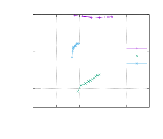
Figure 2 is the plot of accuracy versus entropy score for the balanced case. The different points have been obtained by increasing the support of all the classes simultaneously by the same factor of the total support. As expected, the accuracy increases with the supports, and so the points move from left to right as more data is fed to the models.

We see that the complement model starts with the highest accuracy with the lowest support, but confidence is poor. As we let the supports grow, accuracy grows too and outperform the other models with the same support, but we can also see that the confidence of the complement model stays consistently below the other curves, as it was expected.

Figure 2. The accuracy versus entropy score for the 20 Newsgroup experiment with balanced supports. The left-most points are obtained from models trained with just the 10% of all the samples in each class. Supports are increased in a linear fashion up to 100% of all the samples in each class. As more data is fed into the models, their accuracy increases. However, the confidence of the complement model stays below the other curves.

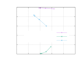
Figure 3 shows similar trends for the unbalanced case. Indeed, with low support, the complement model gives the highest accuracy, but confidence remains poor when compared against the other models. In this particular instance, however, the Binomial model seems to provide better accuracy and confidence scores as the supports increase.

Figure 3. The accuracy versus entropy score for the 20 Newsgroup experiment with unbalanced supports. As in the balanced case, we increase the support size of each class linearly, but we keep relative proportions of roughly $2:5:10$ among the three classes mentioned in the paper. The picture that we get is quite different from the balanced case, but we still spot the poor confidence of the complement model.

The second experiment that we present is different from the first one, in the sense that we have not fixed the classes, but we have set a threshold for the class supports. As a consequence, it is more difficult to compare points on the same curve with each other, but we can still spot the expected behaviour of the complement model.

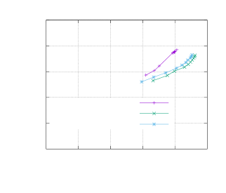
The training data is based on the Wikipedia Movie Plots data set. What we do here is to select all the classes whose support is above a certain threshold. We then repeat the training with increasing values of the threshold to gradually reduce the number of classes that the models see. The training sets are then unbalanced at every run. The result of the experiment is summarised in Figure 4. Again, we move from left to right as the threshold increases (and the number of classes decreases). Contrary to the other two, the complement model shows an upward trend, but as the accuracy grows the confidence attains pretty low values.

Figure 4. The accuracy versus entropy score for the Wikipedia Movie Plots experiment. The threshold values that have been used are 100, 200, 500, 1000. The corresponding numbers of classes that were selected from the training set are 29, 21, 9, 4. Low threshold values then imply more classes and hence lower accuracy (left-ward in the plot). A higher threshold filters out many more classes, thus allowing the models to focus on a restricted pool of choices, yielding better accuracy (rightward in the plot).

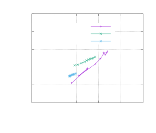
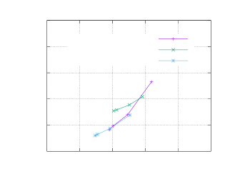
For completeness, we present the results of accuracy vs purity. Based on the analysis of the behaviour of purity as an estimator of confidence, we expect that, as the accuracy grows, the values of purity move from bottom to top. Models that are very confident of the wrong answers will tend to live in the bottom left corner of the plot, whereas models that make good and confident decisions will be located in the top right corner. In the middle we have a horizontal strip, between $0.5$ and $0.7$ of poorly confident models. We can see from the three plots 5, 6 and 7 that the complement models are, as we expected, all located near this middle strip.

Figure 5. The accuracy versus purity for the 20 Newsgroup experiment with balanced supports.

Figure 6. The accuracy versus purity for the 20 Newsgroup experiment with unbalanced supports.

Figure 7. The accuracy versus purity for the Wikipedia Movie Plots experiment.

4. Concluding remarks

It emerges from existing literature that the idea of using entropy to estimate the confidence (or uncertainty) of a probabilistic classifier is, without any doubts, natural and, we could add, almost common sense. Whilst we present the metric (1) as new, we have also observed that, in fact, many authors mention entropy or information when dealing with uncertainty (see, e.g., the already cited [11]). What we have done here was to formalise this idea into the form of a $[0-1]$-metric that can give an estimate of the average confidence of the predictions of a probabilistic classification model.

The applications that we presented showed the usefulness of these metrics both from a practical and a theoretical point of view. Indeed, we made use of the the entropy considerations that are at the heart of the entropy score (1) to provide a theoretical explanation of the degraded confidence observed with the Complement Naïve Bayes model of [4]. On the practical side, we have shown how the accuracy vs entropy score plots can provide a better insight into probabilistic classifiers, especially when decision rules are based on a probability or score threshold. We believe that being able to identify models that are good both in accuracy and confidence is important in those applications where decisions need to be taken only when their confidence is relatively high. For example, one might find that a Multinomial Naïve Bayes model on an unbalanced data set provides satisfactory results in terms of accuracy, and that a decision is taken based on its prediction provided that the probability of the predicted class is above, say, 70%. It is natural to try different models to improve on the accuracy as much as possible, and the Complement Naïve Bayes model of [4] is one way to go. However, one might then find that all the predictions do not go above, say, 30% confidence, meaning that, whilst the model yields higher accuracy, no decision will ever be taken based in its predictions, rendering the “better” model useless.

In this paper we have focused on Naïve Bayes models for the sole purpose of providing a good baseline for comparison against the Complement Naïve Bayes model. Of course, this analysis can be carried out with any probabilistic classifier.

5. Acknowledgements

The author wishes to thank Craig Alexander, Vinny Davies and Martina Pugliese for their valuable comments and suggestions on an earlier draft of this paper.

References

- [1] Pedro Domingos. MetaCost: A general method for making classifiers cost-sensitive. In Proceedings of the Fifth ACM SIGKDD International Conference on Knowledge Discovery and Data Mining, KDD ’99, pages 155–164, New York, NY, USA, 1999. Association for Computing Machinery.
- [2] Tom Fawcett. An introduction to ROC analysis. Pattern Recogn. Lett., 27(8):861–874, 2006.
- [3] F. Pedregosa, G. Varoquaux, A. Gramfort, V. Michel, B. Thirion, O. Grisel, M. Blondel, P. Prettenhofer, R. Weiss, V. Dubourg, J. Vanderplas, A. Passos, D. Cournapeau, M. Brucher, M. Perrot, and E. Duchesnay. Scikit-learn: Machine learning in Python. Journal of Machine Learning Research, 12:2825–2830, 2011.
- [4] Jason D. M. Rennie, Lawrence Shih, Jaime Teevan, and David R. Karger. Tackling the poor assumptions of naive bayes text classifiers. In Proceedings of the Twentieth International Conference on International Conference on Machine Learning, ICML’03, pages 616–623. AAAI Press, 2003.
- [5] Gilbert Ritschard. Computing and using the deviance with classification trees. In Alfredo Rizzi and Maurizio Vichi, editors, Compstat 2006 - Proceedings in Computational Statistics, pages 55–66, Heidelberg, 2006. Physica-Verlag HD.
- [6] Vitaly Schetinin, Derek Partridge, Wojtek J. Krzanowski, Richard M. Everson, Jonathan E. Fieldsend, Trevor C. Bailey, and Adolfo Hernandez. Experimental comparison of classification uncertainty for randomised and bayesian decision tree ensembles. In Zheng Rong Yang, Hujun Yin, and Richard M. Everson, editors, Intelligent Data Engineering and Automated Learning – IDEAL 2004, pages 726–732, Berlin, Heidelberg, 2004. Springer Berlin Heidelberg.
- [7] Kent A. Spackman. Signal detection theory: Valuable tools for evaluating inductive learning. In Proceedings of the Sixth International Workshop on Machine Learning, pages 160–163, San Francisco, CA, USA, 1989. Morgan Kaufmann Publishers Inc.
- [8] Stephen V. Stehman. Selecting and interpreting measures of thematic classification accuracy. Remote Sensing of Environment, 62(1):77–89, 1997.
- [9] Robert Tibshirani. Bias, variance and prediction error for classification rules. University of Toronto, Department of Statistics, 1996.
- [10] Xiao-Ning Wang, Jin-Mao Wei, Han Jin, Gang Yu, and Hai-Wei Zhang. Probabilistic confusion entropy for evaluating classifiers. Entropy, 15(12):4969–4992, Nov 2013.
- [11] Xuchao Zhang, Fanglan Chen, Chang-Tien Lu, and Naren Ramakrishnan. Mitigating uncertainty in document classification. In Proceedings of the 2019 Conference of the North American Chapter of the Association for Computational Linguistics: Human Language Technologies, Volume 1 (Long and Short Papers), pages 3126–3136, Minneapolis, Minnesota, 2019. Association for Computational Linguistics.