TransCenter: Transformers with Dense Representations for Multiple-Object Tracking
Abstract
Transformers have proven superior performance for a wide variety of tasks since they were introduced. In recent years, they have drawn attention from the vision community in tasks such as image classification and object detection. Despite this wave, an accurate and efficient multiple-object tracking (MOT) method based on transformers is yet to be designed. We argue that the direct application of a transformer architecture with quadratic complexity and insufficient noise-initialized sparse queries – is not optimal for MOT. We propose TransCenter, a transformer-based MOT architecture with dense representations for accurately tracking all the objects while keeping a reasonable runtime. Methodologically, we propose the use of image-related dense detection queries and efficient sparse tracking queries produced by our carefully designed query learning networks (QLN). On one hand, the dense image-related detection queries allow us to infer targets’ locations globally and robustly through dense heatmap outputs. On the other hand, the set of sparse tracking queries efficiently interacts with image features in our TransCenter Decoder to associate object positions through time. As a result, TransCenter exhibits remarkable performance improvements and outperforms by a large margin the current state-of-the-art methods in two standard MOT benchmarks with two tracking settings (public/private). TransCenter is also proven efficient and accurate by an extensive ablation study and comparisons to more naive alternatives and concurrent works. For scientific interest, the code is made publicly available at https://github.com/yihongxu/transcenter.
Index Terms:
Multiple-Object Tracking, Efficient Transformer, Dense Image-Related Detection Queries, Sparse Tracking Queries.1 Introduction
The task of tracking multiple objects, usually understood as the simultaneous inference of the positions and identities of various objects/pedestrians (trajectories) in a visual scene recorded by one or more cameras, became a core problem in computer vision in the past years. Undoubtedly, the various multiple-object tracking (MOT) challenges and associated datasets [46, 11], helped foster research on this topic and provided a standard way to evaluate and monitor the performance of the methods proposed by many research teams worldwide.
Recent progress in computer vision using transformers [71] for tasks such as object detection [8, 97, 39], person re-identification (Re-ID) [25] or image super resolution [82], showed the benefit of the attention-based mechanism. Transformers are good at modeling simultaneously dependencies between different parts of the input and thus at making global decisions. These advantages fit perfectly the underlying challenges of MOT, where current methods often struggle when modeling the interaction between objects, especially in crowded scenes. We, therefore, are motivated to investigate the use of a transformer-based architecture for MOT, enabling global estimations when finding trajectories thus reducing missed or noisy predictions of trajectories.
Current MOT methods follow in principle the predominant tracking-by-detection paradigm where we first detect objects in the visual scene and associate them through time. The detection ability is critical for having a good MOT performance. To this end, MOT methods usually combine probabilistic models [55, 3, 41, 2] or deep convolutional architectures [4, 81, 50, 74, 17, 87, 61] with an integrated or external detector to predict bounding-box outputs. They are often based on overlapping predefined anchors that predict redundant outputs, which might create noisy detections, and thus need hand-crafted post-processing techniques such as non-maximum suppression (NMS), which might suppress correct detections. Instead, concurrent MOT methods [65, 45] built on recent object detectors like DETR [8] leverage transformers where sparse noise-initialized queries are employed, which perform cross-attention with encoded images to output one-to-one object-position predictions, thanks to the one-to-one assignment of objects and queries during training. However, using a fixed-number of sparse queries leads to a lack of detections when the visual scene becomes crowded, and the hyper-parameters of the model need to be readjusted. For these reasons, we argue that having dense but non-overlapping representations for detection is beneficial in MOT, especially in crowded scenes.
Indeed, the image-size dense queries are naturally compatible with center heatmap predictions, and there exist center-based MOT methods [94, 89] that output dense object-center heatmap predictions directly related to the input image. Moreover, the center heatmap representations are pixel-related and thus inherit the one-to-one assignment of object centers and queries (pixels) without external assignment algorithms. However, the locality of CNN architecture limits the networks to explore, as transformers do, the co-dependency of objects globally. Therefore, we believe that the transformer-based approach with dense image-related (thus non-overlapping) representations is a better choice for building a powerful MOT method.
Designing such transformer-based MOT with dense image-related representations is far from evident. The main drawback is the computational efficiency related to the quadratic complexity in transformers w.r.t. the dense inputs. To overcome this problem, we introduce TransCenter, with powerful and efficient attention-based encoder and decoder, as well as the query generator.
For the encoder, the DETR [8] structure alleviates this issue by introducing a pre-feature extractor like ResNet-50 to extract lower-scale features before inputting the images to the transformers, but the CNN feature extractor itself contributes to the network complexity. Deformable transformers reduce significantly the attention complexity but the ResNet-50 feature extractor is still kept. Alternatively, recent efficient transformers like [73] discard the pre-feature extractor and input directly image patches, following the ViT structure [13]. They also reduce the attention complexity in transformers by spatial-reduction attention, which makes building efficient transformer-based MOT possible.
In TransCenter Decoder, the use of a deformable transformer indeed reduces the attention complexity. However, with our dense queries, the attention calculation remains heavy, which hinders computational efficiency. Alternatively, our image-size detection queries are generated from the lightweight query learning networks (QLN) that inputs image features from the encoder, and they are already globally related. Therefore, the heavy detection cross-attention with image features can be omitted. Furthermore, The tracking happens in the decoder where we search the current object positions with the known previous ones. With this prior positional information, we design the tracking queries to be sparse, which do not need to search every pixel for finding current object positions and significantly speed up the MOT method without losing accuracy.
To summarize, as roughly illustrated in Fig. 1, TransCenter tackles the MOT problem with image-related dense detection queries and sparse tracking queries. It (i) introduces dense image-related queries to deal with miss detections from insufficient sparse queries or over detections in overlapping anchors of current MOT methods, yielding better MOT accuracy; (ii) solves the efficiency issue inherited in transformers with careful network designs, sparse tracking queries, and removal of useless external overheads, allowing TransCenter to perform MOT efficiently. Overall, this work has the following contributions:
-
•
We introduce TransCenter, the first center-based transformer framework for MOT and among the first to show the benefits of using transformer-based architectures for MOT.
-
•
We carefully explore different network structures to combine the transformer with center representations, specifically proposing dense image-related multi-scale representations that are mutually correlated within the transformer attention and produce abundant but less noisy tracks, while keeping a good computational efficiency.
-
•
We extensively compare with up-to-date online MOT tracking methods, TransCenter sets a new state-of-the-art baseline both in MOT17 [46] (+4.0% Multiple-Object Tracking Accuracy, MOTA) and MOT20 [11] (+18.8% MOTA) by large margins, leading both MOT competitions by the time of our submission in the published literature.
-
•
Moreover, two more model options, TransCenter-Dual, which further boosts the performance in crowded scenes, and TransCenter-Lite, enhancing the computational efficiency, are provided for different requirements in MOT applications.
2 Related Works
2.1 Multiple-Object Tracking
In MOT literature, initial works [3, 55, 1] focus on how to find the optimal associations between detections and tracks through probabilistic models while [47] first formulates the problem as an end-to-end learning task with recurrent neural networks. Moreover, [57] models the dynamics of objects by a recurrent network and further combines the dynamics with an interaction and an appearance branch. [81] proposes a framework to directly use the standard evaluation measures MOTA and MOTP as loss functions to back-propagate the errors for an end-to-end tracking system. [4] employs object detection methods for MOT by modeling the problem as a regression task. A person Re-ID network [68, 4] can be added at the second stage to boost the performance. However, it is still not optimal to treat the Re-ID as a secondary task. [89] further proposes a framework that treats the person detection and Re-ID tasks equally and [48] uses quasi-dense proposals from anchor-based detectors to learn Re-ID features for MOT in a dense manner. [63] proposes a fast online MOT with detection refinement. Motion clues in MOT are also important since a well-designed motion model can compensate for missing detections due to occlusions. To this end, [83] unifies the motion and affinity models for MOT. [43] leverages articulation information to perform MOT. [58, 22] focus on the motion-based interpolation based on probabilistic models. [78] unifies the segmentation and detection task in an MOT framework combining historic tracking information as a strong clue for the data association. Derived from the success in single-object tracking, [64] employs siamese networks for MOT. [88] simply leverages low-score detections to explore partially occluded objects. Moreover, traditional graphs are also used to model the positions of objects as nodes and the temporal connection of the objects as edges [26, 68, 66, 32, 67]. The performance of those methods is further boosted by the recent rise of Graph Neural Networks (GNNs): hand-designed graphs are replaced by learnable GNNs [76, 77, 74, 49, 7, 23] to model the complex interaction of the objects.
Most of the above methods follow the tracking by detections/regression paradigm where a detector provides detections for tracking. The paradigm has proven state-of-the-art performance with the progress in object detectors. Unlike classic anchor-based detectors [54, 53], recent progress in keypoint-based detectors [35, 95] exhibited better performance while discarding overlapping and manually-designed box anchors trying to cover all possible object shapes and positions. Built on keypoint-based detectors, [94], [89] and [93] represent objects as centers in a heatmap then reason about all the objects jointly and associate them across adjacent frames with a tracking branch or Re-ID branch.
2.2 Transformers in Multiple-Object Tracking
Transformer is first proposed by [71] for machine translation and has shown its ability to handle long-term complex dependencies between entries in a sequence by using a multi-head attention mechanism. With its success in natural language processing, works in computer vision start to investigate transformers for various tasks, such as image recognition [13], Person Re-ID [25], realistic image generation [29], super-resolution [82] and audio-visual learning [16, 15].
Object detection with Transformer (DETR) [8] can be seen as an exploration and correlation task. It is an encoder-decoder structure where the encoder extracts the image information and the decoder finds the best correlation between the object queries and the encoded image features with an attention module. The attention module transforms the inputs into Query (), Key (), and Value () with fully-connected layers. Having , the attended features are calculated with the attention function [71]:
| (1) |
where is the hidden dimension of and . The attention calculation suffers from heavy computational and memory complexities w.r.t the input size: the feature maps extracted from a ResNet-50 [24] backbone are used to alleviate the problem. Deformable DETR [97] further tackles the issue by proposing deformable attention inspired by [10], drastically speeding up the convergence (10) and reducing the complexity. The reduction of memory consumption allows in practice using multi-scale features to capture finer details, yielding better detection performance. However, the CNN backbone is still kept in Deformable DETR. This important overhead hinders the Transformer from being efficient. Alternatively, Pyramid Vision Transformer [73] (PVT) extracts the visual features directly from the input images and the attention is calculated with efficient spatial-reduction attention (SRA). Precisely, PVT follows the ViT [13] structure while the feature maps are gradually down-scaled with a patch embedding module (with convolutional layers and layer normalization). To reduce the quadratic complexity of Eq. 1 w.r.t the dimension of , the SRA in PVT reduces beforehand the dimension of from to (with , the scaling factor) and keeps the dimension of unchanged. The complexity can be reduced by times while the dimension of the output attended features remains unchanged, boosting the efficiency of transformer attention modules.
The use of transformers is still recent in MOT. Before transformers, some attempts with simple attention-based modules have been introduced for MOT. Specifically, [21] proposes a target and distractor-aware attention module to produce more reliable appearance embeddings, which also helps suppress detection drift and [72] proposes hand-designed spatial and temporal correlation modules to achieve long-range information similar to what transformers inherit. After the success in detection using transformers, two concurrent works directly apply transformers on MOT based on the (deformable) DETR framework. First, Trackformer [45] builds directly from DETR [8] and is trained to propagate the queries through time. Second, Transtrack [65] extends [97] to MOT by adding a decoder that processes the features at to refine previous detection positions. Importantly, both methods stay in the DETR framework with sparse queries and extend it for tracking. However, recent literature [94, 89, 93] also suggests that point-based tracking may be a better option for MOT while the use of pixel-level dense queries with transformers to predict dense heatmaps for MOT has never been studied. In addition, we question the direct transfer from DETR to MOT as concurrent works do [65, 45]. Indeed, the sparse queries without positional correlations might be problematic in two folds. Firstly, the insufficient number of queries could cause severe miss detections thus false negatives (FN) in tracking. Secondly, queries are highly overlapping, and simply increasing the number of non-positional-correlated queries may end up having many false detections and false positives (FP) in tracking. All of the above motivates us to investigate a better transformer-based MOT framework. We thus introduce TransCenter a methodology that takes existing drawbacks into account at the design level and achieves state-of-the-art performance.
3 TransCenter
TransCenter tackles the detection and temporal association in MOT accurately and efficiently. Different from concurrent transformer-based MOT methods, TransCenter questions the use of sparse queries without image correlations (i.e. noise initialized), and explores the use of image-related dense queries, producing dense representations using transformers. To that aim, we introduce the query learning networks (QLN) responsible for converting the outputs of the encoder into the inputs of the TransCenter Decoder. Different possible architectures for QLN and TransCenter Decoder are proposed, and the choice is made based on both the accuracy and the efficiency aspects.
While exploiting dense representations from dense queries111See visualization in Supplementary Material Sec. B.2., can help to sufficiently detect the objects, especially in crowded scenes, the design of dense queries is not trivial. Notably, the quadratic increase of calculation complexity in transformers should be solved, and the noise tracks from randomly initialized dense queries should be addressed. To this end, we propose image-related dense queries, which have three prominent advantages: (1) the queries are multi-scale and exploit the multi-resolution structure of the encoder, allowing for very small targets to be captured by those queries; (2) image-related dense detection queries also make the network more flexible. The number of queries grows with the input resolution. No fixed hyper-parameters like in [65] need to be adjusted to re-train the model, which depends on the density of objects in the scene; (3) the query-pixel correspondence discards the time-consuming Hungarian matching [34] for the query-ground-truth object association. Up to our knowledge, we are the first to explore the use of image-related dense detection queries that scale with the input image size. Meanwhile, we solve the efficiency issue through a careful network design that appropriately handles the dense representation of queries, which provides an accurate and efficient MOT method.
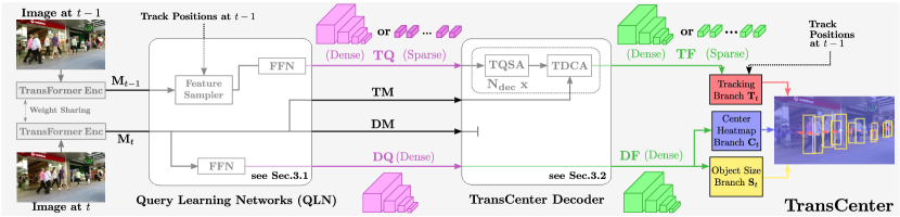
A generic pipeline of TransCenter is illustrated in Fig. 2. RGB images at and are input to the weight-shared transformer encoder from which dense multi-scale attended features are obtained, namely memories and . They are the inputs of the QLN. QLN produces two sets of output pairs, detection queries () and memory () for detecting the objects at time , and tracking queries () and memory () for associating the objects at with previous time step . Furthermore, TransCenter Decoder, leveraging the deformable transformer [97], is used to correlate / with /. To elaborate, interacts with in the cross-attention module of the TransCenter Decoder, resulting in the tracking features (). Similarly, the detection features () are the output of the cross-attention between and . To produce the output dense representations, are used to estimate the object size and the center heatmap . Meanwhile are used to estimate the tracking displacement .
One can argue that the downside of using dense queries is the associated higher memory consumption and lower computational efficiency. One drawback with previous or concurrent approaches is the use of the deformable DETR encoder including the CNN feature extractor ResNet-50 [24], which significantly slows down the feature extraction. Instead, TransCenter leverages PVTv2 [73] as its encoder, the so-called PVT-Encoder. The reasons are three-fold: (1) it discards the ResNet-50 backbone and uses efficient attention heads [73], reducing significantly the network complexity; (2) it has flexible scalability by modifying the feature dimension and block structures. Specifically, we use B0 (denoted as PVT-Lite) in TransCenter-Lite and B2 (PVT-Encoder) for TransCenter and TransCenter-Dual, see details in [73] and Sec.4.1; (3) its feature pyramid structure is suitable for building dense pixel-level multi-scale queries.
Once the transformer encoder extracts the dense memory representations and , they are passed to QLN and then to the TransCenter Decoder. We carefully search the design choices of QLN (see Sec. 3.1) and TransCenter Decoder (see Sec. 3.2), and select the best model based on the efficiency and accuracy. In particular, we demonstrate that can be sparse 222See visualization in Supplementary Material Sec. B.3., different from , since we have the prior information of object positions at the previous time step that helps to search their corresponding positions at the current time step. Therefore, it is not necessary to search every pixel for this aim. Consequently, the discretization of tracking queries based on previous object positions (roughly from 14k to less than 500 depending on the number of objects) can significantly speed up the tracking attention calculation in the TransCenter Decoder.
Regarding the detection, the cross attention module between the dense detection queries () and the detection memory () is beneficial in terms of performance but at the cost of significant computational loads. We solve this by studying the impact of the detection cross-attention on the computational efficiency and the accuracy. We introduce two variants of the proposed method, TransCenter-Dual and TransCenter-Lite. The former shares the same structure as TransCenter but having DDCA for detection in the decoder, as detailed in Sec. 3.2; The latter is a lighter version of TransCenter with a lighter encoder (PVT-Lite).
In the following sections, we detail the design choices of the QLN and the TransCenter Decoder, and provide the details of the final output branches (see Sec. 3.3) as well as the training losses (see Sec. 3.4).
3.1 QLN: Query Learning Networks
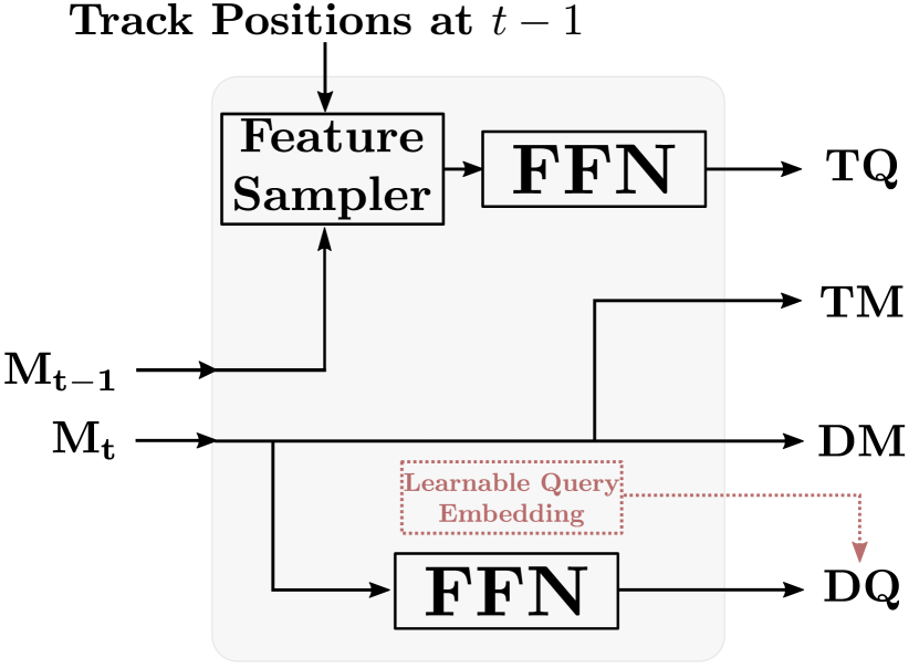
QLN are networks that relate the queries and the memories. In our design, (1) are dense and image-related that discover object positions precisely and abundantly. (2) Different from , are sparse and aim at finding object displacements between two different frames, and thus and should be produced by input features from different time steps.
Based on these attributes, we design the chosen QLNS-333”S” means sparse, ”” means that the features are sampled from . It is counter-intuitive to have QLNS because at time , we know neither the number of tracked objects (tracks) at nor their positions, we cannot thus sample features with track positions. that produces by passing (attended features from image ) through a FFN (feed-forward network with fully-connected layers). For , QLNS- samples object features with a feature sampler using bilinear interpolation from using object positions at , while outputting from features at a different time step, . Moreover, different possible variants of QLN are visualized in Fig. 3 and are summarized as follows:
-
1.
QLND-: QLNS- with dense (with the subscript ”D”) without the feature sampler.
-
2.
QLN: QLND- with dense from and from .
-
3.
QLNDQ: QLND- with dense from and from .
-
4.
QLNE: QLNDQ with noise-initialized learnable embeddings (with the subscript ”E”).
-
5.
QLNSE-: QLNS- with noise-initialized learnable embeddings for detection.
In Sec. 4.5, different QLN are carefully designed and ablated to produce dense detection queries relative to the input image and sparse tracking queries for accurate and efficient MOT with transformers.
3.2 TransCenter Decoder
To successfully find object trajectories, a MOT method should not only detect the objects but also associate them across frames. To do so, TransCenter Decoder tackles in parallel the two sub-tasks: detection and object temporal association (tracking). Concretely, TransCenter Decoder consists of Tracking Deformable Cross-Attention (TDCA), and Detection Deformable Cross-Attention (DDCA) modules. Moreover, Tracking Query Self-Attention (TQSA) module is introduced to enhance the interactions among sparse tracking queries through a multi-head self-attention, knowing that the overhead is acceptable because the tracking queries are sparse in TransCenter. TDCA calculates cross attention between tracking queries and memories ( and ), resulting in tracking features (). Analogously, DDCA calculates cross attention between detection queries and memories ( and ), producing detection features (). Deformable cross attention module [97] with linear complexity w.r.t. input size is used.
From the efficiency perspective, the use of the multi-head attention modules in traditional transformers [71] like DETR [8] implies a complexity growth that is quadratic with the input size. Of course, this is undesirable and would limit the scalability and usability of the method. To mitigate this, we resort to the deformable multi-head attention [97]–Deformable Cross-Attention (DCA), where the queries are input to produce sampling offsets for displacing the input reference points. The reference points are from either the track position at for tracking in TDCA or the pixel coordinates of the dense queries for detection in DDCA666The reference points are omitted in the figures for simplicity.. The displaced coordinates are used to locate and sample features in or . The input queries also produce in DCA the attention weights for merging sampled features. However, the cost of calculating the cross attention between and is still not negligible because of their multi-scale image resolutions. To solve this, we demonstrate in Sec. 4.5 (Single v.s. Dual decoder) that it is possible to output directly as for output-branch predictions, with an acceptable loss of accuracy as expected. In addition, under this sparse nature of in TransCenter, we enhance the interactions among queries by adding lightweight TQSA before TDCA.
To conclude, we choose to use a TQSA-Single TransCenter Decoder for the cross attention of and while we directly use for the output branches. This is possible thanks to the sparse and dense , which yields a good balance between computational efficiency and accuracy, The overall Decoder design is illustrated in Fig. 5 and the comparison between different design choices can be found in Sec. 4.5.
3.3 The Center, the Size, and the Tracking Branches
Given and from the TransCenter Decoder, we use them as the input of different branches to output object center heatmap , their box size and the tracking displacements . contain feature maps of four different resolutions, namely , and of the input image resolution. For the center heatmap and the object size, the feature maps at different resolutions are combined using deformable convolutions [10] and bilinear interpolation up-sampling, following the architecture shown in Fig. 5. They are up-sampled into a feature map of of the input resolution and then input to and . and are the input image height and width, respectively, and the two channels of encode the object size in width and height.
Regarding the tracking branch, the tracking features are sparse having the same size as the number of tracks at . One tracking query feature corresponds to one track at . , together with object positions at ( in the case of sparse ) or center heatmap and (dense ), are input to two fully-connected layers with ReLU activation. The latter layers predict the horizontal and vertical displacements of objects at in the adjacent frames.
3.4 Model Training
The model training is achieved by jointly learning a 2D classification task for the object center heatmap and a regression task for the object size and tracking displacements, covering the branches of TransCenter. For the sake of clarity, in this section, we will drop the time index . Center Focal Loss. To train the center branch, we need first to build the ground-truth heatmap response . As done in [94], we construct by considering the maximum response of a set of Gaussian kernels centered at each of the ground-truth object centers. More formally, for every pixel position the ground-truth heatmap response is computed as:
| (2) |
where is the ground-truth object center, and is the Gaussian kernel with spread . In our case, is proportional to the object’s size, as described in [35]. Given the ground-truth and the inferred center heatmaps, the center focal loss, is formulated as:
| (3) |
where the scaling factors are and , see [89]. Sparse Regression Loss. The values of is supervised only on the locations where object centers are present, i.e. using a loss:
| (4) |
The formulation of for is analogous to but using the tracking output and ground-truth displacement, instead of the object size. To complete the sparsity of , we add an extra regression loss, denoted as with the bounding boxes computed from and ground-truth centers. To summarize, the overall loss is formulated as the weighted sum of all the losses, where the weights are chosen according to the numeric scale of each loss:
| (5) |
4 Experimental Evaluation
4.1 Implementation Details
Inference with TransCenter. Once the method is trained, we detect objects by selecting the maximum responses from the output center heatmap . Since the datasets are annotated with bounding boxes, we need to convert our estimates into this representation. In detail, we apply (after max pooling) a threshold (e.g. 0.3 for MOT17 and 0.4 for MOT20 in TransCenter) to the center heatmap, thus producing a list of center positions . We extract the object size associated to each position in . The set of detections produced by TransCenter is denoted as . In parallel, for associating objects through frames (tracking), given the position of an object at , we can estimate the object position in the current frame by extracting the corresponding displacement estimate from . Therefore, we can construct a set of tracked positions . Finally, we use the Hungarian algorithm [34] to match the tracked positions – and the detection at – . The matched detections are used to update the tracked object positions at . The birth and death processes are naturally integrated in TransCenter: detections not associated with any tracked object give birth to new tracks, while unmatched tracks are put to sleep for at most frames before being discarded. An external Re-ID network is often used in MOT methods [4] to recover tracks in sleep, which is proven unnecessary in our experiment in Sec. 4.5. We also assess inference speed in fps in the testset results either obtained from [88] or tested under the same GPU setting. Network and Training Parameters. The input images are resized to with padding in TransCenter and TransCenter-Dual while it is set to in TransCenter-Lite. In TransCenter, the PVT-Encoder has layers ( in PVT-Lite) for each image feature scale and the corresponding hidden dimension ( in PVT-Lite). for the TransCenter Decoder with eight attention heads and six layers (four layers in TransCenter-Lite). All TransCenter models are trained with loss weights , and by the AdamW optimizer [44] with learning rate . The training converges at around 50 epochs, applying a learning rate decay of at the 40th epoch. The entire network is pre-trained on the pedestrian class of COCO [40] and then fine-tuned on the respective MOT dataset [46, 11]. We also present the results finetuned with extra data like CrowdHuman dataset [62] (see Sec. 4.3 for details).
| Public Detections | Private Detections | |||||||||||||||||||
| Method | Data | MOTA | MOTP | IDF1 | MT | ML | FP | FN | IDS | FPS | Data | MOTA | MOTP | IDF1 | MT | ML | FP | FN | IDS | FPS |
| MOTDT17 [9] | \cellcolororange!12re1 | \cellcolororange!1250.9 | \cellcolororange!1276.6 | \cellcolororange!1252.7 | \cellcolororange!1217.5 | \cellcolororange!1235.7 | \cellcolororange!1224,069 | \cellcolororange!12250,768 | \cellcolororange!122,474 | \cellcolororange!1218.3 | \cellcolorblack!12 | \cellcolorblack!12 | \cellcolorblack!12 | \cellcolorblack!12 | \cellcolorblack!12 | \cellcolorblack!12 | \cellcolorblack!12 | \cellcolorblack!12 | \cellcolorblack!12 | \cellcolorblack!12 |
| *UnsupTrack [30] | \cellcolororange!12pt | \cellcolororange!1261.7 | \cellcolororange!1278.3 | \cellcolororange!1258.1 | \cellcolororange!1227.2 | \cellcolororange!1232.4 | \cellcolororange!1216,872 | \cellcolororange!12197,632 | \cellcolororange!121,864 | \cellcolororange!1217.5 | \cellcolorblack!12 | \cellcolorblack!12 | \cellcolorblack!12 | \cellcolorblack!12 | \cellcolorblack!12 | \cellcolorblack!12 | \cellcolorblack!12 | \cellcolorblack!12 | \cellcolorblack!12 | \cellcolorblack!12 |
| GMT_CT [23] | \cellcolororange!12re2 | \cellcolororange!1261.5 | \cellcolorblack!12 | \cellcolororange!1266.9 | \cellcolororange!1226.3 | \cellcolororange!1232.1 | \cellcolororange!1214,059 | \cellcolororange!12200,655 | \cellcolororange!122,415 | \cellcolorblack!12 | \cellcolorblack!12 | \cellcolorblack!12 | \cellcolorblack!12 | \cellcolorblack!12 | \cellcolorblack!12 | \cellcolorblack!12 | \cellcolorblack!12 | \cellcolorblack!12 | \cellcolorblack!12 | \cellcolorblack!12 |
| TrackFormer [45] | \cellcolororange!12ch | \cellcolororange!1262.5 | \cellcolorblack!12 | \cellcolororange!1260.7 | \cellcolororange!1229.8 | \cellcolororange!1226.9 | \cellcolororange!1214,966 | \cellcolororange!12206,619 | \cellcolororange!121,189 | \cellcolororange!126.8 | \cellcolorblack!12 | \cellcolorblack!12 | \cellcolorblack!12 | \cellcolorblack!12 | \cellcolorblack!12 | \cellcolororange!12\cellcolorblack!12 | \cellcolorblack!12 | \cellcolororange!12\cellcolorblack!12 | \cellcolorblack!12 | \cellcolorblack!12 |
| SiamMOT [64] | \cellcolororange!12ch | \cellcolororange!1265.9 | \cellcolorblack!12 | \cellcolororange!1263.5 | \cellcolororange!1234.6 | \cellcolororange!1223.9 | \cellcolororange!1218,098 | \cellcolororange!12170,955 | \cellcolororange!123,040 | \cellcolororange!1212.8 | \cellcolorblack!12 | \cellcolorblack!12 | \cellcolorblack!12 | \cellcolorblack!12 | \cellcolorblack!12 | \cellcolorblack!12 | \cellcolorblack!12 | \cellcolorblack!12 | \cellcolorblack!12 | \cellcolorblack!12 |
| *MOTR [85] | \cellcolororange!12ch | \cellcolororange!1267.4 | \cellcolorblack!12 | \cellcolororange!1267.0 | \cellcolororange!1234.6 | \cellcolororange!1224.5 | \cellcolororange!1232,355 | \cellcolororange!12149,400 | \cellcolororange!121,992 | \cellcolororange!127.5 | \cellcolorblack!12 | \cellcolorblack!12 | \cellcolorblack!12 | \cellcolorblack!12 | \cellcolorblack!12 | \cellcolorblack!12 | \cellcolorblack!12 | \cellcolorblack!12 | \cellcolorblack!12 | \cellcolorblack!12 |
| TrackFormer [45] | \cellcolorblack!12 | \cellcolorblack!12 | \cellcolorblack!12 | \cellcolorblack!12 | \cellcolorblack!12 | \cellcolorblack!12 | \cellcolorblack!12 | \cellcolorblack!12 | \cellcolorblack!12 | \cellcolorblack!12 | \cellcolororange!12ch | \cellcolororange!1265.0 | \cellcolorblack!12 | \cellcolororange!1263.9 | \cellcolororange!1245.6 | \cellcolororange!1213.8 | \cellcolororange!1270,443 | \cellcolororange!12123,552 | \cellcolororange!123,528 | \cellcolororange!126.8 |
| CenterTrack [94] | \cellcolorblack!12 | \cellcolorblack!12 | \cellcolorblack!12 | \cellcolorblack!12 | \cellcolorblack!12 | \cellcolorblack!12 | \cellcolorblack!12 | \cellcolorblack!12 | \cellcolorblack!12 | \cellcolorblack!12 | \cellcolororange!12ch | \cellcolororange!1267.8 | \cellcolororange!1278.4 | \cellcolororange!1264.7 | \cellcolororange!1234.6 | \cellcolororange!1224.6 | \cellcolororange!1218,489 | \cellcolororange!12160,332 | \cellcolororange!123,039 | \cellcolororange!1217.5 |
| TraDeS [78] | \cellcolorblack!12 | \cellcolorblack!12 | \cellcolorblack!12 | \cellcolorblack!12 | \cellcolorblack!12 | \cellcolorblack!12 | \cellcolorblack!12 | \cellcolorblack!12 | \cellcolorblack!12 | \cellcolorblack!12 | \cellcolororange!12ch | \cellcolororange!1269.1 | \cellcolorblack!12 | \cellcolororange!1263.9 | \cellcolororange!1236.4 | \cellcolororange!1221.5 | \cellcolororange!1220,892 | \cellcolororange!12150,060 | \cellcolororange!123,555 | \cellcolororange!1217.5 |
| PermaTrack [70] | \cellcolorblack!12 | \cellcolorblack!12 | \cellcolorblack!12 | \cellcolorblack!12 | \cellcolorblack!12 | \cellcolorblack!12 | \cellcolorblack!12 | \cellcolorblack!12 | \cellcolorblack!12 | \cellcolorblack!12 | \cellcolororange!12ch | \cellcolororange!1273.8 | \cellcolorblack!12 | \cellcolororange!1268.9 | \cellcolororange!1243.8 | \cellcolororange!1217.2 | \cellcolororange!1228,998 | \cellcolororange!12114,104 | \cellcolororange!123,699 | \cellcolororange!1211.9 |
| *TransTrack [65] | \cellcolorblack!12 | \cellcolorblack!12 | \cellcolorblack!12 | \cellcolorblack!12 | \cellcolorblack!12 | \cellcolorblack!12 | \cellcolorblack!12 | \cellcolorblack!12 | \cellcolorblack!12 | \cellcolorblack!12 | \cellcolororange!12ch | \cellcolororange!1274.5 | \cellcolororange!1280.6 | \cellcolororange!1263.9 | \cellcolororange!1246.8 | \cellcolororange!1211.3 | \cellcolororange!1228,323 | \cellcolororange!12112,137 | \cellcolororange!123,663 | \cellcolororange!1210.0 |
| TransCenter | \cellcolororange!12ch | \cellcolororange!1275.9 | \cellcolororange!1281.2 | \cellcolororange!1265.9 | \cellcolororange!1249.8 | \cellcolororange!1212.1 | \cellcolororange!1230,190 | \cellcolororange!12100,999 | \cellcolororange!124,626 | \cellcolororange!1211.7 | \cellcolororange!12ch | \cellcolororange!1276.2 | \cellcolororange!1281.1 | \cellcolororange!1265.5 | \cellcolororange!1253.5 | \cellcolororange!127.9 | 40,101\cellcolororange!12 | \cellcolororange!1288,827 | \cellcolororange!125,394 | \cellcolororange!1211.8 |
| GSDT [74] | \cellcolorblack!12 | \cellcolorblack!12 | \cellcolorblack!12 | \cellcolorblack!12 | \cellcolorblack!12 | \cellcolorblack!12 | \cellcolorblack!12 | \cellcolorblack!12 | \cellcolorblack!12 | \cellcolorblack!12 | \cellcolorred!125d1 | \cellcolorred!1266.2 | \cellcolorred!1279.9 | \cellcolorred!1268.7 | \cellcolorred!1240.8 | \cellcolorred!1218.3 | \cellcolorred!1243,368 | \cellcolorred!12144,261 | \cellcolorred!123,318 | \cellcolorred!124.9 |
| SOTMOT [93] | \cellcolorred!125d1 | \cellcolorred!1262.8 | \cellcolorblack!12 | \cellcolorred!12 67.4 | \cellcolorred!1224.4 | \cellcolorred!1233.0 | \cellcolorred!126,556 | \cellcolorred!12201,319 | \cellcolorred!122,017 | \cellcolorred!1216.0 | \cellcolorred!125d1 | \cellcolorred!1271.0 | \cellcolorblack!12 | \cellcolorred!1271.9 | \cellcolorred!1242.7 | \cellcolorred!1215.3 | \cellcolorred!1239,537 | \cellcolorred!12118,983 | \cellcolorred!125,184 | \cellcolorred!1216.0 |
| GSDT_V2 [74] | \cellcolorblack!12 | \cellcolorblack!12 | \cellcolorblack!12 | \cellcolorblack!12 | \cellcolorblack!12 | \cellcolorblack!12 | \cellcolorblack!12 | \cellcolorblack!12 | \cellcolorblack!12 | \cellcolorblack!12 | \cellcolorred!125d1 | \cellcolorred!1273.2 | \cellcolorblack!12 | \cellcolorred!1266.5 | \cellcolorred!1241.7 | \cellcolorred!1217.5 | \cellcolorred!1226,397 | \cellcolorred!12120,666 | \cellcolorred!123,891 | \cellcolorred!124.9 |
| CorrTracker [72] | \cellcolorblack!12 | \cellcolorblack!12 | \cellcolorblack!12 | \cellcolorblack!12 | \cellcolorblack!12 | \cellcolorblack!12 | \cellcolorblack!12 | \cellcolorblack!12 | \cellcolorblack!12 | \cellcolorblack!12 | \cellcolorred!125d1 | \cellcolorred!1276.5 | \cellcolorblack!12 | \cellcolorred!1273.6 | \cellcolorred!1247.6 | \cellcolorred!1212.7 | \cellcolorred!1229,808 | \cellcolorred!12 99,510 | \cellcolorred!123,369 | \cellcolorred!1215.6 |
| FairMOT [89] | \cellcolorblack!12 | \cellcolorblack!12 | \cellcolorblack!12 | \cellcolorblack!12 | \cellcolorblack!12 | \cellcolorblack!12 | \cellcolorblack!12 | \cellcolorblack!12 | \cellcolorblack!12 | \cellcolorblack!12 | \cellcolorred!125d1+CH | \cellcolorred!1273.7 | \cellcolorred!1281.3 | \cellcolorred!1272.3 | \cellcolorred!1243.2 | \cellcolorred!1217.3 | \cellcolorred!1227,507 | \cellcolorred!12117,477 | \cellcolorred!123,303 | \cellcolorred!1225.9 |
| *RelationTrack [84] | \cellcolorblack!12 | \cellcolorblack!12 | \cellcolorblack!12 | \cellcolorblack!12 | \cellcolorblack!12 | \cellcolorblack!12 | \cellcolorblack!12 | \cellcolorblack!12 | \cellcolorblack!12 | \cellcolorblack!12 | \cellcolorred!125d1+CH | \cellcolorred!1273.8 | \cellcolorred!1281.0 | \cellcolorred!1274.7 | \cellcolorred!1241.7 | \cellcolorred!1223.2 | \cellcolorred!1227,999 | \cellcolorred!12118,623 | \cellcolorred!121,374 | \cellcolorred!127.4 |
| CSTrack [38] | \cellcolorblack!12 | \cellcolorblack!12 | \cellcolorblack!12 | \cellcolorblack!12 | \cellcolorblack!12 | \cellcolorblack!12 | \cellcolorblack!12 | \cellcolorblack!12 | \cellcolorblack!12 | \cellcolorblack!12 | \cellcolorred!125d1+CH | \cellcolorred!1274.9 | \cellcolorred!1280.9 | \cellcolorred!1272.6 | \cellcolorred!1241.5 | \cellcolorred!1217.5 | \cellcolorred!1223,847 | \cellcolorred!12114,303 | \cellcolorred!123,567 | \cellcolorred!1215.8 |
| MLT [87] | \cellcolorblack!12 | \cellcolorblack!12 | \cellcolorblack!12 | \cellcolorblack!12 | \cellcolorblack!12 | \cellcolorblack!12 | \cellcolorblack!12 | \cellcolorblack!12 | \cellcolorblack!12 | \cellcolorblack!12 | \cellcolorred!12(5d1+CH) | \cellcolorred!1275.3 | \cellcolorred!1281.7 | \cellcolorred!1275.5 | \cellcolorred!1249.3 | \cellcolorred!1219.5 | \cellcolorred!1227,879 | \cellcolorred!12109,836 | \cellcolorred!121,719 | \cellcolorred!125.9 |
| *FUFET [61] | \cellcolorblack!12 | \cellcolorblack!12 | \cellcolorblack!12 | \cellcolorblack!12 | \cellcolorblack!12 | \cellcolorblack!12 | \cellcolorblack!12 | \cellcolorblack!12 | \cellcolorblack!12 | \cellcolorblack!12 | \cellcolorred!12(5d1+CH) | \cellcolorred!1276.2 | \cellcolorred!1281.1 | \cellcolorred!1268.0 | \cellcolorred!1251.1 | \cellcolorred!1213.6 | \cellcolorred!1232,796 | \cellcolorred!1298,475 | \cellcolorred!123,237 | \cellcolorred!126.8 |
| TransCenter | \cellcolorred!125d1+CH | \cellcolorred!1276.0 | \cellcolorred!1281.4 | \cellcolorred!1265.6 | \cellcolorred!1247.3 | \cellcolorred!1215.3 | \cellcolorred!1228,369 | \cellcolorred!12101,988 | \cellcolorred!124,972 | \cellcolorred!1211.7 | \cellcolorred!125d1+CH | \cellcolorred!1276.4 | \cellcolorred!1281.2 | \cellcolorred!1265.4 | \cellcolorred!1251.7 | \cellcolorred!1211.6 | \cellcolorred!1237,005 | \cellcolorred!1289,712 | \cellcolorred!126,402 | \cellcolorred!1210.9 |
| TrctrD17 [81] | \cellcolorgreen!12no | \cellcolorgreen!1253.7 | \cellcolorgreen!1277.2 | \cellcolorgreen!1253.8 | \cellcolorgreen!1219.4 | \cellcolorgreen!1236.6 | \cellcolorgreen!1211,731 | \cellcolorgreen!12247,447 | \cellcolorgreen!121,947 | \cellcolorgreen!122.0 | \cellcolorblack!12 | \cellcolorblack!12 | \cellcolorblack!12 | \cellcolorblack!12 | \cellcolorblack!12 | \cellcolorblack!12 | \cellcolorblack!12 | \cellcolorblack!12 | \cellcolorblack!12 | \cellcolorblack!12 |
| Tracktor [4] | \cellcolorgreen!12no | \cellcolorgreen!1253.5 | \cellcolorgreen!1278.0 | \cellcolorgreen!1252.3 | \cellcolorgreen!1219.5 | \cellcolorgreen!1236.6 | \cellcolorgreen!1212,201 | \cellcolorgreen!12248,047 | \cellcolorgreen!122,072 | \cellcolorgreen!122.0 | \cellcolorblack!12 | \cellcolorblack!12 | \cellcolorblack!12 | \cellcolorblack!12 | \cellcolorblack!12 | \cellcolorblack!12 | \cellcolorblack!12 | \cellcolorblack!12 | \cellcolorblack!12 | \cellcolorblack!12 |
| Tracktor++ [4] | \cellcolorgreen!12no | \cellcolorgreen!1256.3 | \cellcolorgreen!1278.8 | \cellcolorgreen!1255.1 | \cellcolorgreen!1221.1 | \cellcolorgreen!1235.3 | \cellcolorgreen!128,866 | \cellcolorgreen!12235,449 | \cellcolorgreen!121,987 | \cellcolorgreen!122.0 | \cellcolorblack!12 | \cellcolorblack!12 | \cellcolorblack!12 | \cellcolorblack!12 | \cellcolorblack!12 | \cellcolorblack!12 | \cellcolorblack!12 | \cellcolorblack!12 | \cellcolorblack!12 | \cellcolorblack!12 |
| GSM_Tracktor [42] | \cellcolorgreen!12no | \cellcolorgreen!1256.4 | \cellcolorgreen!1277.9 | \cellcolorgreen!1257.8 | \cellcolorgreen!1222.2 | \cellcolorgreen!1234.5 | \cellcolorgreen!1214,379 | \cellcolorgreen!12230,174 | \cellcolorgreen!121,485 | \cellcolorgreen!128.7 | \cellcolorblack!12 | \cellcolorblack!12 | \cellcolorblack!12 | \cellcolorblack!12 | \cellcolorblack!12 | \cellcolorblack!12 | \cellcolorblack!12 | \cellcolorblack!12 | \cellcolorblack!12 | \cellcolorblack!12 |
| TADAM [21] | \cellcolorgreen!12no | \cellcolorgreen!1259.7 | \cellcolorblack!12 | \cellcolorgreen!1258.7 | \cellcolorblack!12 | \cellcolorblack!12 | \cellcolorgreen!129,676 | \cellcolorgreen!12216,029 | \cellcolorgreen!121,930 | \cellcolorblack!12 | \cellcolorblack!12 | \cellcolorblack!12 | \cellcolorblack!12 | \cellcolorblack!12 | \cellcolorblack!12 | \cellcolorblack!12 | \cellcolorblack!12 | \cellcolorblack!12 | \cellcolorblack!12 | \cellcolorblack!12 |
| CenterTrack [94] | \cellcolorgreen!12no | \cellcolorgreen!1261.5 | \cellcolorgreen!1278.9 | \cellcolorgreen!1259.6 | \cellcolorgreen!1226.4 | \cellcolorgreen!1231.9 | \cellcolorgreen!1214,076 | \cellcolorgreen!12200,672 | \cellcolorgreen!122,583 | \cellcolorgreen!1217.5 | \cellcolorblack!12 | \cellcolorblack!12 | \cellcolorblack!12 | \cellcolorblack!12 | \cellcolorblack!12 | \cellcolorblack!12 | \cellcolorblack!12 | \cellcolorblack!12 | \cellcolorblack!12 | \cellcolorblack!12 |
| *FUFET [61] | \cellcolorgreen!12no | \cellcolorgreen!1262.0 | \cellcolorblack!12 | \cellcolorgreen!1259.5 | \cellcolorgreen!1227.8 | \cellcolorgreen!1231.5 | \cellcolorgreen!1215,114 | \cellcolorgreen!12196,672 | \cellcolorgreen!122,621 | \cellcolorgreen!126.8 | \cellcolorblack!12 | \cellcolorblack!12 | \cellcolorblack!12 | \cellcolorblack!12 | \cellcolorblack!12 | \cellcolorblack!12 | \cellcolorblack!12 | \cellcolorblack!12 | \cellcolorblack!12 | \cellcolorblack!12 |
| ArTIST-C [58] | \cellcolorgreen!12no | \cellcolorgreen!1262.3 | \cellcolorblack!12 | \cellcolorgreen!1259.7 | \cellcolorgreen!1229.1 | \cellcolorgreen!1234.0 | \cellcolorgreen!1219,611 | \cellcolorgreen!12191,207 | \cellcolorgreen!122,062 | \cellcolorgreen!1217.5 | \cellcolorblack!12 | \cellcolorblack!12 | \cellcolorblack!12 | \cellcolorblack!12 | \cellcolorblack!12 | \cellcolorblack!12 | \cellcolorblack!12 | \cellcolorblack!12 | \cellcolorblack!12 | \cellcolorblack!12 |
| MAT [22] | \cellcolorgreen!12no | \cellcolorgreen!1267.1 | \cellcolorgreen!1280.8 | \cellcolorgreen!1269.2 | \cellcolorgreen!1238.9 | \cellcolorgreen!1226.4 | \cellcolorgreen!1222,756 | \cellcolorgreen!12161,547 | \cellcolorgreen!121,279 | \cellcolorgreen!129.0 | \cellcolorblack!12 | \cellcolorblack!12 | \cellcolorblack!12 | \cellcolorblack!12 | \cellcolorblack!12 | \cellcolorblack!12 | \cellcolorblack!12 | \cellcolorblack!12 | \cellcolorblack!12 | \cellcolorblack!12 |
| MTP [33] | \cellcolorgreen!12no | \cellcolorgreen!1251.5 | \cellcolorblack!12 | \cellcolorgreen!1254.9 | \cellcolorgreen!1220.5 | \cellcolorgreen!1235.5 | \cellcolorgreen!1229,623 | \cellcolorgreen!12241,618 | \cellcolorgreen!122,563 | \cellcolorgreen!1220.1 | \cellcolorgreen!12no | \cellcolorgreen!1255.9 | \cellcolorblack!12 | \cellcolorgreen!1260.4 | \cellcolorgreen!1220.5 | \cellcolorgreen!1236.7 | \cellcolorgreen!128,653 | \cellcolorgreen!12238,853 | \cellcolorgreen!121,188 | \cellcolorgreen!1220.1 |
| ChainedTracker [50] | \cellcolorblack!12 | \cellcolorblack!12 | \cellcolorblack!12 | \cellcolorblack!12 | \cellcolorblack!12 | \cellcolorblack!12 | \cellcolorblack!12 | \cellcolorblack!12 | \cellcolorblack!12 | \cellcolorblack!12 | \cellcolorgreen!12no | \cellcolorgreen!1266.6 | \cellcolorgreen!1278.2 | \cellcolorgreen!1257.4 | \cellcolorgreen!1232.2 | \cellcolorgreen!1224.2 | \cellcolorgreen!1222,284 | \cellcolorgreen!12160,491 | \cellcolorgreen!125,529 | \cellcolorgreen!126.8 |
| QDTrack [48] | \cellcolorgreen!12no | \cellcolorgreen!1264.6 | \cellcolorgreen!1279.6 | \cellcolorgreen!1265.1 | \cellcolorgreen!1232.3 | \cellcolorgreen!1228.3 | \cellcolorgreen!1214,103 | \cellcolorgreen!1218,2998 | \cellcolorgreen!122,652 | \cellcolorgreen!1220.3 | \cellcolorgreen!12no | \cellcolorgreen!1268.7 | \cellcolorgreen!1279.0 | \cellcolorgreen!1266.3 | \cellcolorgreen!1240.6 | \cellcolorgreen!1221.9 | \cellcolorgreen!1226,589 | \cellcolorgreen!1214,6643 | \cellcolorgreen!123,378 | \cellcolorgreen!1220.3 |
| TransCenter | \cellcolorgreen!12no | \cellcolorgreen!1271.9 | \cellcolorgreen!1280.5 | \cellcolorgreen!1264.1 | \cellcolorgreen!1244.4 | \cellcolorgreen!1218.6 | \cellcolorgreen!1227,356 | \cellcolorgreen!12126,860 | \cellcolorgreen!124,118 | \cellcolorgreen!1211.9 | \cellcolorgreen!12no | \cellcolorgreen!1272.7 | \cellcolorgreen!1280.3 | \cellcolorgreen!1264.0 | \cellcolorgreen!1248.7 | \cellcolorgreen!1214.0 | \cellcolorgreen!1233,807 | \cellcolorgreen!12115,542 | \cellcolorgreen!124,719 | \cellcolorgreen!1211.8 |
4.2 Protocol
Datasets and Detections. We use the standard split of the MOT17 [46] and MOT20 [11] datasets and the testset evaluation is obtained by submitting the results to the MOTChallenge website. The MOT17 testset contains 2,355 trajectories distributed in 17,757 frames. MOT20 testset contains 1,501 trajectories within only 4,479 frames, which leads to a much more challenging crowded-scene setting. We evaluate TransCenter both under public and private detections. When using public detections, we limit the maximum number of birth candidates at each frame to the number of public detections per frame, as in [94, 45]. The selected birth candidates are those closest to the public detections with IOU larger than 0. When using private detections, there are no constraints, and the detections depend only on the network’s detection capacity, the use of external detectors, and more importantly, the use of extra training data. For this reason, we regroup the results by the use of extra training datasets as detailed in the following. In addition, we evaluate our TransCenter on the KITTI dataset under the autonomous driving setting. KITTI dataset contains annotations of cars and pedestrians in 21 and 29 video sequences in the training and test sets, respectively. For the results of KITTI dataset, we use also [69] as extra data.
| Public Detections | Private Detections | |||||||||||||||||||
| Method | Data | MOTA | MOTP | IDF1 | MT | ML | FP | FN | IDS | FPS | Data | MOTA | MOTP | IDF1 | MT | ML | FP | FN | IDS | FPS |
| *UnsupTrack [30] | \cellcolororange!12pt | \cellcolororange!1253.6 | \cellcolororange!1280.1 | \cellcolororange!1250.6 | \cellcolororange!1230.3 | \cellcolororange!1225.0 | \cellcolororange!126,439 | \cellcolororange!12231,298 | \cellcolororange!122,178 | \cellcolororange!1217.5 | \cellcolorblack!12 | \cellcolorblack!12 | \cellcolorblack!12 | \cellcolorblack!12 | \cellcolorblack!12 | \cellcolorblack!12 | \cellcolorblack!12 | \cellcolorblack!12 | \cellcolorblack!12 | \cellcolorblack!12 |
| *TransTrack [65] | \cellcolorblack!12 | \cellcolorblack!12 | \cellcolorblack!12 | \cellcolorblack!12 | \cellcolorblack!12 | \cellcolorblack!12 | \cellcolorblack!12 | \cellcolorblack!12 | \cellcolorblack!12 | \cellcolorblack!12 | \cellcolororange!12ch | \cellcolororange!1264.5 | \cellcolororange!1280.0 | \cellcolororange!1259.2 | \cellcolororange!1249.1 | \cellcolororange!1213.6 | \cellcolororange!1228,566 | \cellcolororange!12151,377 | \cellcolororange!123,565 | \cellcolororange!127.2 |
| TransCenter | \cellcolororange!12ch | \cellcolororange!1272.8 | \cellcolororange!1281.0 | \cellcolororange!1257.6 | \cellcolororange!1265.5 | \cellcolororange!1212.1 | \cellcolororange!1228,026 | \cellcolororange!12110,312 | \cellcolororange!122,621 | \cellcolororange!128.4 | \cellcolororange!12ch | \cellcolororange!1272.9 | \cellcolororange!1281.0 | \cellcolororange!1257.7 | \cellcolororange!1266.5 | \cellcolororange!1211.8 | \cellcolororange!1228,596 | \cellcolororange!12108,982 | \cellcolororange!122,625 | \cellcolororange!128.7 |
| CorrTracker [72] | \cellcolorblack!12 | \cellcolorblack!12 | \cellcolorblack!12 | \cellcolorblack!12 | \cellcolorblack!12 | \cellcolorblack!12 | \cellcolorblack!12 | \cellcolorblack!12 | \cellcolorblack!12 | \cellcolorblack!12 | \cellcolorred!125d1 | \cellcolorred!1265.2 | \cellcolorblack!12 | \cellcolorred!1269.1 | \cellcolorred!1266.4 | \cellcolorred!128.9 | \cellcolorred!1279,429 | \cellcolorred!1295,855 | \cellcolorred!125,183 | \cellcolorred!128.5 |
| GSDT_V2 [74] | \cellcolorblack!12 | \cellcolorblack!12 | \cellcolorblack!12 | \cellcolorblack!12 | \cellcolorblack!12 | \cellcolorblack!12 | \cellcolorblack!12 | \cellcolorblack!12 | \cellcolorblack!12 | \cellcolorblack!12 | \cellcolorred!125d1 | \cellcolorred!1267.1 | \cellcolorblack!12 | \cellcolorred!1267.5 | \cellcolorred!1253.1 | \cellcolorred!1213.2 | \cellcolorred!1231,507 | \cellcolorred!12135,395 | \cellcolorred!123,230 | \cellcolorred!120.9 |
| GSDT [74] | \cellcolorblack!12 | \cellcolorblack!12 | \cellcolorblack!12 | \cellcolorblack!12 | \cellcolorblack!12 | \cellcolorblack!12 | \cellcolorblack!12 | \cellcolorblack!12 | \cellcolorblack!12 | \cellcolorblack!12 | \cellcolorred!125d1 | \cellcolorred!1267.1 | \cellcolorred!1279.1 | \cellcolorred!1267.5 | \cellcolorred!1253.1 | \cellcolorred!1213.2 | \cellcolorred!1231,913 | \cellcolorred!12135,409 | \cellcolorred!123,131 | \cellcolorred!120.9 |
| SOTMOT [93] | \cellcolorblack!12 | \cellcolorblack!12 | \cellcolorblack!12 | \cellcolorblack!12 | \cellcolorblack!12 | \cellcolorblack!12 | \cellcolorblack!12 | \cellcolorblack!12 | \cellcolorblack!12 | \cellcolorblack!12 | \cellcolorred!125d1 | \cellcolorred!1268.6 | \cellcolorblack!12 | \cellcolorred!1271.4 | \cellcolorred!1264.9 | \cellcolorred!129.7 | \cellcolorred!1257,064 | \cellcolorred!12101,154 | \cellcolorred!124,209 | \cellcolorred!128.5 |
| FairMOT [89] | \cellcolorblack!12 | \cellcolorblack!12 | \cellcolorblack!12 | \cellcolorblack!12 | \cellcolorblack!12 | \cellcolorblack!12 | \cellcolorblack!12 | \cellcolorblack!12 | \cellcolorblack!12 | \cellcolorblack!12 | \cellcolorred!125d1+CH | \cellcolorred!1261.8 | \cellcolorred!1278.6 | \cellcolorred!1267.3 | \cellcolorred!1268.8 | \cellcolorred!127.6 | \cellcolorred!12103,440 | \cellcolorred!1288,901 | \cellcolorred!125,243 | \cellcolorred!1213.2 |
| CSTrack [38] | \cellcolorblack!12 | \cellcolorblack!12 | \cellcolorblack!12 | \cellcolorblack!12 | \cellcolorblack!12 | \cellcolorblack!12 | \cellcolorblack!12 | \cellcolorblack!12 | \cellcolorblack!12 | \cellcolorblack!12 | \cellcolorred!125d1+CH | \cellcolorred!1266.6 | \cellcolorred!1278.8 | \cellcolorred!1268.6 | \cellcolorred!1250.4 | \cellcolorred!1215.5 | \cellcolorred!1225,404 | \cellcolorred!12144,358 | \cellcolorred!123,196 | \cellcolorred!124.5 |
| *RelationTrack [84] | \cellcolorblack!12 | \cellcolorblack!12 | \cellcolorblack!12 | \cellcolorblack!12 | \cellcolorblack!12 | \cellcolorblack!12 | \cellcolorblack!12 | \cellcolorblack!12 | \cellcolorblack!12 | \cellcolorblack!12 | \cellcolorred!125d1+CH | \cellcolorred!1267.2 | \cellcolorred!1279.2 | \cellcolorred!1270.5 | \cellcolorred!1262.2 | \cellcolorred!128.9 | \cellcolorred!1261,134 | \cellcolorred!12104,597 | \cellcolorred!124,243 | \cellcolorred!122.7 |
| TransCenter | \cellcolorred!125d1+CH | \cellcolorred!1272.4 | \cellcolorred!1281.2 | \cellcolorred!1257.9 | \cellcolorred!1264.2 | \cellcolorred!1212.3 | \cellcolorred!1225,121 | \cellcolorred!12115,421 | \cellcolorred!122,290 | \cellcolorred!128.6 | \cellcolorred!125d1+CH | \cellcolorred!1272.5 | \cellcolorred!1281.1 | \cellcolorred!1258.1 | \cellcolorred!1264.7 | \cellcolorred!1212.2 | \cellcolorred!1225,722 | \cellcolorred!12114,310 | \cellcolorred!122,332 | \cellcolorred!128.8 |
| SORT [6] | \cellcolorgreen!12no | \cellcolorgreen!1242.7 | \cellcolorgreen!1278.5 | \cellcolorgreen!1245.1 | \cellcolorgreen!1216.7 | \cellcolorgreen!1226.2 | \cellcolorgreen!1227,521 | \cellcolorgreen!12264,694 | \cellcolorgreen!124,470 \cellcolorgreen!12 | \cellcolorgreen!12 27.7 | \cellcolorblack!12 | \cellcolorblack!12 | \cellcolorblack!12 | \cellcolorblack!12 | \cellcolorblack!12 | \cellcolorblack!12 | \cellcolorblack!12 | \cellcolorblack!12 | \cellcolorblack!12 | \cellcolorblack!12 |
| Tracktor++ [4] | \cellcolorgreen!12no | \cellcolorgreen!1252.6 | \cellcolorgreen!1279.9 | \cellcolorgreen!1252.7 | \cellcolorgreen!1229.4 | \cellcolorgreen!1226.7 | \cellcolorgreen!126,930 | \cellcolorgreen!12236,680 | \cellcolorgreen!121,648 | \cellcolorgreen!121.2 | \cellcolorblack!12 | \cellcolorblack!12 | \cellcolorblack!12 | \cellcolorblack!12 | \cellcolorblack!12 | \cellcolorblack!12 | \cellcolorblack!12 | \cellcolorblack!12 | \cellcolorblack!12 | \cellcolorblack!12 |
| ArTIST-T [58] | \cellcolorgreen!12no | \cellcolorgreen!1253.6 | \cellcolorblack!12 | \cellcolorgreen!1251.0 | \cellcolorgreen!1231.6 | \cellcolorgreen!1228.1 | \cellcolorgreen!127,765 | \cellcolorgreen!12230,576 | \cellcolorgreen!121,531 | \cellcolorgreen!121.2 | \cellcolorblack!12 | \cellcolorblack!12 | \cellcolorblack!12 | \cellcolorblack!12 | \cellcolorblack!12 | \cellcolorblack!12 | \cellcolorblack!12 | \cellcolorblack!12 | \cellcolorblack!12 | \cellcolorblack!12 |
| GNNMatch [49] | \cellcolorgreen!12no | \cellcolorgreen!1254.5 | \cellcolorgreen!1279.4 | \cellcolorgreen!1249.0 | \cellcolorgreen!1232.8 | \cellcolorgreen!1225.5 | \cellcolorgreen!129,522 | \cellcolorgreen!12223,611 | \cellcolorgreen!122,038 | \cellcolorgreen!120.1 | \cellcolorblack!12 | \cellcolorblack!12 | \cellcolorblack!12 | \cellcolorblack!12 | \cellcolorblack!12 | \cellcolorblack!12 | \cellcolorblack!12 | \cellcolorblack!12 | \cellcolorblack!12 | \cellcolorblack!12 |
| TADAM [21] | \cellcolorgreen!12no | \cellcolorgreen!1256.6 | \cellcolorblack!12 | \cellcolorgreen!1251.6 | \cellcolorblack!12 | \cellcolorblack!12 | \cellcolorgreen!1239,407 | \cellcolorgreen!1218,2520 | \cellcolorgreen!122,690 | \cellcolorblack!12 | \cellcolorblack!12 | \cellcolorblack!12 | \cellcolorblack!12 | \cellcolorblack!12 | \cellcolorblack!12 | \cellcolorblack!12 | \cellcolorblack!12 | \cellcolorblack!12 | \cellcolorblack!12 | \cellcolorblack!12 |
| MLT [87] | \cellcolorblack!12 | \cellcolorblack!12 | \cellcolorblack!12 | \cellcolorblack!12 | \cellcolorblack!12 | \cellcolorblack!12 | \cellcolorblack!12 | \cellcolorblack!12 | \cellcolorblack!12 | \cellcolorblack!12 | \cellcolorgreen!12no | \cellcolorgreen!1248.9 | \cellcolorgreen!1278.0 | \cellcolorgreen!1254.6 | \cellcolorgreen!1230.9 | \cellcolorgreen!1222.1 | \cellcolorgreen!1245,660 | \cellcolorgreen!12216,803 | \cellcolorgreen!122,187 | \cellcolorgreen!123.7 |
| TransCenter | \cellcolorgreen!12no | \cellcolorgreen!12 67.7 | \cellcolorgreen!1279.8 | \cellcolorgreen!1258.9 | \cellcolorgreen!1265.6 | \cellcolorgreen!1211.3 | \cellcolorgreen!1254,967 | \cellcolorgreen!12108,376 | \cellcolorgreen!123,707 | \cellcolorgreen!128.4 | \cellcolorgreen!12no | \cellcolorgreen!12 67.7 | \cellcolorgreen!1279.8 | \cellcolorgreen!1258.7 | \cellcolorgreen!1266.3 | \cellcolorgreen!1211.1 | \cellcolorgreen!1256,435 | \cellcolorgreen!12107,163 | \cellcolorgreen!123,759 | \cellcolorgreen!128.4 |
Extra Training Data. To fairly compare with the state-of-the-art methods, we denote the extra data used to train each method, including several pre-prints listed in the MOTChallenge leaderboard, which are marked with * in our result tables777COCO [40] and ImageNet [28] are not considered as extra data according to the MOTchallenge [46, 11].: ch for CrowdHuman [62], pt for PathTrack [59], re1 for the combination of Market1501 [91], CUHK01 and CUHK03 [36] person re-identification datasets, re2 replaces CUHK01 [36] with DukeMTMC [56], 5d1 for the use of five extra datasets (ETH [14], Caltech Pedestrian [12, 51], CityPersons [86], CUHK-SYS [80], and PRW [92]), 5d1+CH is the same as 5d1 plus CroudHuman. (5d1+CH) uses the tracking/detection results of FairMOT [89] trained within the 5d1+CH setting, and no stands for using no extra dataset. Metrics. Standard MOT metrics such as MOTA (Multiple Object Tracking Accuracy) and MOTP (Multiple Object Tracking Precision) [5] are used: MOTA is mostly used since it reflects the average tracking performance including the number of FP (False positives, predicted bounding boxes not enclosing any object), FN (False negatives, missing ground-truth objects) and IDS [37] (Identities of predicted trajectories switch through time). MOTP evaluates the quality of bounding boxes from successfully tracked objects. Moreover, we also evaluate IDF1 [56] (the ratio of correctly identified detections over the average number of ground-truth objects and predicted tracks), MT (the ratio of ground-truth trajectories that are covered by a track hypothesis more than 80% of their life span), and ML (less than 20% of their life span).
4.3 Testset Results and Discussion
MOT17. Tab. I presents the results obtained in the MOT17 testset. The first global remark is that most state-of-the-art methods do not evaluate under both public and private detections, and under different extra-training data settings, while we do. Secondly, TransCenter sets new state-of-the-art performance compared to other methods, in terms of MOTA, under CH and no-extra training data conditions, both for public and private detections. Precisely, the increase of MOTA w.r.t. the state-of-the-art methods is of and (both including unpublished methods by now) for the public detection setting under CH and no-extra training data, and of and for the private detection setting, respectively. The superiority of TransCenter is remarkable in most of the metrics. We can also observe that TransCenter trained with no extra-training data outperforms, not only the methods trained with no extra data but also some methods trained with one extra dataset. Similarly, TransCenter trained on ch performs better than seven methods trained with five or more extra datasets in the private setting, comparable to the best result in 5d1+ch (-0.3% MOTA), showing that TransCenter is less data-hungry. Moreover, trained with 5d1+ch, the performance is further improved while running at around 11 fps. Overall, these results confirm our hypothesis that TransCenter with dense detection representations and sparse tracking representations produced by global relevant queries in transformers is a better choice. MOT20. Tab. II reports the results obtained in MOT20 testset. In all settings, similar to the case in MOT17, TransCenter leads the competition by a large margin compared to all the other methods. Concretely, TransCenter outperforms current methods by +19.2%/+8.4% in MOTA with the public/private setting trained with ch and +11.1%/18.8% without extra data. From the results, another remarkable achievement of TransCenter is the significant decrease of FN while keeping a relatively low FP number. This indicates that the dense representation of the detection queries can help effectively detect objects sufficiently and accurately. As for tracking, TransCenter maintains low IDS numbers in MOT20 running at around 8 fps in such crowded scenes, thanks to our careful choices of QLN and the TransCenter Decoder. Very importantly, to the best of our knowledge, our study is the first to report the results of all settings on MOT20, demonstrating the tracking capacity of TransCenter even in a densely crowded scenario. The outstanding results of TransCenter in MOT20 further show the effectiveness of our design.
| Method | MOTA | MOTP | FP | FN | IDS | FPS | |
| Car | MASS [31] | 84.6 | 85.4 | 4,145 | 786 | 353 | 100.0 |
| IMMDP [79] | 82.8 | 82.8 | 5,300 | 422 | 211 | 5.3 | |
| AB3D [75] | 83.5 | 85.2 | 4,492 | 1,060 | 126 | 214.7 | |
| SMAT [20] | 83.6 | 85.9 | 5,254 | 175 | 198 | 10.0 | |
| TrackMPNN [52] | 87.3 | 84.5 | 2,577 | 1,298 | 481 | 20.0 | |
| CenterTrack [94] | 88.8 | 85.0 | 2,703 | 886 | 254 | 22.2 | |
| TransCenter | 87.3 | 83.8 | 3,189 | 847 | 340 | 18.5 | |
| Person | AB3D [75] | 38.9 | 64.6 | 11,744 | 2,135 | 259 | 214.7 |
| TrackMPNN [52] | 52.1 | 73.4 | 7,705 | 2,758 | 626 | 20.0 | |
| CenterTrack [94] | 53.8 | 73,7 | 8,061 | 2,201 | 425 | 22.2 | |
| TransCenter | 59.1 | 73.2 | 6,889 | 2,142 | 436 | 18.5 |
KITTI. Additionally, we show the results of TransCenter evaluated on the KITTI dataset. TransCenter significantly outperforms CenterTrack [94] in pedestrian tracking (+5.3% MOTA) while keeping a close performance in car tracking. However, the KITTI dataset is constructed in an autonomous driving scenario with only up to 15 cars and 30 pedestrians per image but some of the sequences contain no pedestrians. The sparse object locations cannot fully show the capacity of TransCenter to detect and track densely crowded objects.
4.4 Efficiency-Accuracy Tradeoff Discussion
| Model | Enc/Det | #params (M) | IM (MB) | FPS | MOTA | |
| MOT-17 | FairMOT [89] | DLA-34 | 20.3 | 892 | 25.9 | 73.7 |
| CenterTrack [94] | 20.0 | 892 | 17.5 | 67.8 | ||
| TrackFormer [45] | D. DETR | 40.0 | 976 | 6.8 | 65.0 | |
| TransTrack [65] | 47.1 | 1,002 | 10.0 | 74.5 | ||
| TransCenter-DETR | 43.6 | 980 | 8.8 | 74.8 | ||
| ByteTrack [88] | YOLOX | 99.1 | 1,746 | 29.6 | 80.3 | |
| MO3TR-PIQ [96]888100 noise-initialized learnable queries. | N/A | N/A | N/A | 77.6 | ||
| TransCenter-YOLOX | 35.1 | 938 | 11.9 | 79.8 | ||
| TransCenter-Dual | PVT | 39.7 | 954 | 5.6 | 76.0 | |
| TransCenter | 35.1 | 938 | 11.8 | 76.2 | ||
| TransCenter-Lite | 8.1 | 838 | 17.5 | 73.5 | ||
| ByteTrack | Pub. Det. | 99.1 | 1,746 | N/A | 67.4 | |
| TransCenter | 35.1 | 938 | 11.7 | 75.9 | ||
| MOT-20 | FairMOT [89] | DLA-34 | 20.3 | 892 | 13.2 | 61.8 |
| CenterTrack [94] | N/A | N/A | N/A | N/A | ||
| TrackFormer [45] | D. DETR | N/A | N/A | N/A | N/A | |
| TransTrack [65] | 47.1 | 1,002 | 7.2 | 64.5 | ||
| TransCenter-DETR | 43.6 | 980 | 7.5 | 68.8 | ||
| ByteTrack [88] | YOLOX | 99.1 | 1,746 | 17.5 | 77.8 | |
| MO3TR-PIQ [96] | N/A | N/A | N/A | 72.3 | ||
| TransCenter-YOLOX | 35.1 | 938 | 10.1 | 77.9 | ||
| TransCenter-Dual | PVT | 39.7 | 954 | 5.1 | 73.5 | |
| TransCenter | 35.1 | 938 | 8.7 | 72.9 | ||
| TransCenter-Lite | 8.1 | 838 | 11.0 | 68.0 | ||
| ByteTrack | Pub. Det. | 99.1 | 1,746 | N/A | 67.0 | |
| TransCenter | 35.1 | 938 | 8.4 | 72.8 |
To have a direct idea of the better design of TransCenter, we discuss in detail the efficiency-accuracy tradeoff comparing TransCenter, TransCenter-Lite, and TransCenter-Dual to the transformer-based concurrent works – TransTrack [65] and TrackFormer [45]. To have a fairer comparison to these methods using the (deformable) DETR encoder (D. DETR), i.e. ResNet-50 with a deformable transformer encoder, we leverage TransCenter-DETR, having the same encoder as theirs while keeping the rest of its structure unchanged. Moreover, related to our method, we show superior performance compared to the center-based MOT methods – CenterTrack [94] and FairMOT [89]. The comparisons take into account the number of model parameters, the model memory footprint during inference, the inference speed (frame per second or FPS), and the MOTA performance as shown in Tab. IV, completed with Tab. I and Tab. II. Additionally, we compare the center heatmap/query responses of the aforementioned methods in Sec. B.1 of the Supplementary Material, showing that TransCenter produces sufficient and accurate outputs.
Very recently, works like ByteTrack [88] and MO3TR-PIQ [96] take advantage of the recent off-the-shelf object detector YOLOX [18] trained with extensive data-augmentation tricks such as MixUp [90], which significantly improves the MOT performance. However, we do not think that the MOT performance improvement from the object detector could be considered as their contribution to the MOT community. Even though, for the scientific interest, we use the results of the YOLOX from ByteTrack [88] as matching and birth candidates to show that TransCenter can have a similar or even better result compared to ByteTrack and MO3TR-PIQ [96], denoted as TransCenter-YOLOX. 77footnotetext: MO3TR-PIQ [96] is not yet published and does not provide source code nor sufficient information to evaluate the IM, #params, and the FPS.
All results are evaluated on both MOT17 and MOT20 testsets in the private detection setting except the comparison with ByteTrack in the public detection setting (see Pub. Det. in Tab. IV). All the models are pretrained on CrowdHuman [62] except for FairMOT [89] trained also on 5d1+ch datasets, and ByteTrack additionally trained on ETH [14] and CityPersons [86]. The default input image size for CenterTrack [94] is , for FairMOT [89] and TransCenter-Lite, for TransCenter TransCenter-Dual, TransCenter-DETR and TransCenter-YOLOX. TrackFormer [45] and TransTrack [65] use varying input sizes with short size of ; ByteTrack [88] uses an input size of . Compared to Transformer-Based MOT. With the respect to our concurrent works, we compare TransCenter to them both in accuracy and inference speed. Unfortunately, Trackformer [45] by far only shows results on MOT17 and TransTrack [65] does not show results in all settings. One important remark is that TransCenter systematically outperforms TransTrack and TrackFormer in both accuracy (MOTA) and speed (FPS) with a smaller model size (# of model parameters) and less inference memory consumption in all settings. Precisely, using the same training data, TransCenter exhibits better performance compared TransTrack by +1.7% MOTA (by +11.2% v.s. TrackFormer) in MOT17 and significantly by +8.4% in MOT20. The PVT [73] encoder can indeed bring faster inference speed and provide more meaningful image features that boost the MOT performance. However, using the same encoder as TransTrack, TransCenter-DETR exhibits similar inference speed and much better performance in both MOT20 (+4.3%) and MOT17 (+0.3%), compared to TransTrack. This indicates that the overall design of TransCenter is more efficient and powerful. Moreover, we recall that, unlike our concurrent works, TransCenter leverages pixel-level dense and multi-scale detection queries to predict dense center-based heatmaps, mitigating the miss-tracking problem while keeping relatively good computational efficiency with sparse tracking queries, efficient QLN, and TransCenter Decoder. TransCenter demonstrates thus a significantly better efficiency-accuracy tradeoff. Finally, for different MOT applications, we provide TransCenter-Dual, introduced to further boost the performance in crowded scenes, and TransCenter-Lite for efficiency-critical applications.
Compared to Center-Based MOT. With the long-term dependencies and the dense interactions of queries in transformers, unlike pure CNN-based center MOT methods, our queries interact globally with each other and make global decisions. TransCenter exhibits much better accuracy compared to previous center-based MOT methods, CenterTrack and FairMOT [94, 89]. Precisely as shown in Tab. I and Tab. IV, TransCenter tracks more and better compared to CenterTrack, with +8.4% (+10.4%) MOTA and -71,505 (-73,812) FN in MOT17 private (public) detections, using the same dense center representations and trained with the same data. CenterTrack does not show results in MOT20 while FairMOT, similar to CenterTrack, shows good results in MOT20. It alleviates miss detections by training with much more data, leading to much fewer FN but producing much noisier detections (FP). Surprisingly, with much less training data (CH), TransCenter still outperforms by a large margin [89] (+11.1% MOTA shown in Tab. IV) even in very crowded MOT20, with cleaner detections (suppressing -74,844 FP) and better tracking associations (-2,618 IDS) shown in Tab. II. Indeed, the inference speed is slower compared to CNN-based methods, but the above comparisons have demonstrated that previous center-based MOT methods are not comparable in terms of accuracy to TransCenter, with an acceptable fps around 11 fps for MOT17 and 8 fps for MOT20. Moreover, to adapt to applications with more strict inference constraints, TransCenter-Lite is introduced, keeping a better performance while having competitive inference speed compared to center-based MOT methods.
Compared to YOLOX-Based MOT. The recent works ByteTrack [88] and MO3TR-PIQ show significant performance gain by using the off-the-shelf object detector YOLOX [18]. We believe that the gain is mainly from the object detector, which is not the contribution of any aforementioned method. This claim is further confirmed by the direct comparison of TransCenter and ByteTrack in public detection, i.e. without YOLOX, where TransCenter outperforms the latter with 75.9% v.s. 67.4% MOTA in MOT17 and 72.8% v.s. 67.0% in MOT20 (see Tab. IV).
For private detection, to have a fair comparison with them, we use the detection results from YOLOX (same as ByteTrack) to demonstrate that YOLOX can also significantly boost TransCenter in terms of MOTA. Precisely, TransCenter-YOLOX shows +2.2% MOTA compared to MO3TR-PIQ while only having a 0.5% difference compared to ByteTrack in MOT17. We remind that ByteTrack is an offline method with offline post-processing interpolation. In very crowded scenes like MOT20, TransCenter-YOLOX outperforms MO3TR-PIQ and ByteTrack by +5.6% and +0.1% in MOTA respectively. We agree that indeed there is an inference speed discrepancy with CNN-based methods compared to our transformer-based TransCenter. However, in terms of accuracy, TransCenter-YOLOX shows comparable or even better results, compared to all other methods. This indicates that the design of TransCenter is beneficial with different encoders/object detectors.
To conclude, TransCenter expresses both better accuracy and efficiency compared to transformer-based methods [65, 45]; much higher accuracy numbers and competitive efficiency compared to [94, 89], showing better efficiency-accuracy balance. Moreover, with the powerful YOLOX detector, TransCenter can be significantly improved in terms of MOT performance, showing the potential of TransCenter.
| Settings | MOT17 | MOT20 | ||||||||||||||
| Line | Encoder | Decoder | Queries | QLN | MOTA | IDF1 | FP | FN | IDS | FPS | MOTA | IDF1 | FP | FN | IDS | FPS |
| 1 | DETR | Dual | \cellcolorblack!12S-S99943,520 noise-initialized learnable queries. | \cellcolorblack!12QLNE | 49.4 | 49.6 | 4,909 | 8,202 | 602 | 2.5 | 42.5 | 26.8 | 19,243 | 153,429 | 4,375 | 1.5 |
| 2 | DETR | Dual | \cellcolorblack!12D-D101010Like other MOT methods, we observe that clipping the box size within the image size for tracking results in MOT20 improves slightly the MOTA performance. To have a fair comparison, all the results in MOT20 are updated with this technique. | \cellcolorblack!12QLNE | 56.6 | 50.1 | 3,510 | 7,577 | 678 | 1.7 | 67.3 | 32.1 | 45,547 | 46,962 | 8,115 | 0.9 |
| 3 | DETR | Dual | \cellcolorblack!12D-D | \cellcolorblack!12QLNDQ | 69.2 | 71.9 | 1,202 | 6,951 | 203 | 1.9 | 79.41111footnotemark: 11 | 66.9 | 7,697 | 53,987 | 1,680 | 1.2 |
| 4 | DETR | Dual | D-D | \cellcolorblack!12QLN | 66.8 | 71.2 | 1,074 | 7,757 | 167 | 1.9 | 78.3 | 64.7 | 5517 | 59,447 | 1,832 | 1.2 |
| 5 | DETR | Dual | D-D | \cellcolorblack!12QLND- | 65.8 | 70.3 | 1,122 | 7,987 | 176 | 1.9 | 78.4 | 64.2 | 5,340 | 59,288 | 1,798 | 1.1 |
| 6 | DETR | Dual | D-D | \cellcolorblack!12QLNDQ | 69.2 | 71.9 | 1,202 | 6,951 | 203 | 1.9 | 79.4 | 66.9 | 7,697 | 53,987 | 1,680 | 1.2 |
| 7 | \cellcolorblack!12DETR | Single | D-D | QLNDQ | 68.1 | 72.0 | 580 | 7,922 | 141 | 2.1 | 79.8 | 66.9 | 6,955 | 53,445 | 1,657 | 1.2 |
| 8 | \cellcolorblack!12PVT | Single | D-D | QLNDQ | 72.3 | 71.4 | 1,116 | 6,156 | 249 | 8.1 | 83.6 | 75.1 | 14,358 | 34,782 | 1,348 | 6.1 |
| 9∗ | \cellcolorblack!12PVT-Lite | Single | D-S | QLNS- | 69.8 | 71.6 | 2,008 | 5,923 | 252 | 19.4 | 82.9 | 75.5 | 14,857 | 36,510 | 1,181 | 12.4 |
| 10∗ | \cellcolorblack!12PVT | TQSA-Single | D-S | QLNS- | 73.8 | 74.1 | 1,302 | 5,540 | 258 | 12.4 | 83.6 | 75.7 | 15,459 | 34,054 | 1,085 | 8.9 |
| 11∗ | PVT | \cellcolorblack!12TQSA-Dual | D-S | QLNS- | 74.6 | 76.5 | 892 | 5,879 | 128 | 5.6 | 84.6 | 78.0 | 13,415 | 33,202 | 921 | 4.8 |
| 12∗ | PVT | \cellcolorblack!12TQSA-Single | D-S | QLNS- | 73.8 | 74.1 | 1,302 | 5,540 | 258 | 12.4 | 83.6 | 75.7 | 15,459 | 34,054 | 1,085 | 8.9 |
| 13 | PVT | \cellcolorblack!12Single | D-S | QLNS- | 69.4 | 72.5 | 1,756 | 6,335 | 197 | 13.3 | 83.0 | 74.7 | 14,584 | 36,441 | 1,321 | 9.8 |
| 14∗ | PVT | \cellcolorblack!12TQSA-Single | D-S | QLNS- | 73.8 | 74.1 | 1,302 | 5,540 | 258 | 12.4 | 83.6 | 75.7 | 15,459 | 34,054 | 1,085 | 8.9 |
| 15 | PVT | Single | \cellcolorblack!12D-D | QLND- | 71.1 | 71.7 | 1,274 | 6,274 | 278 | 9.0 | 82.5 | 75.0 | 12,686 | 40,003 | 1,216 | 6.3 |
| 16∗ | PVT | TQSA-Single | \cellcolorblack!12D-S | QLNS- | 73.8 | 74.1 | 1,302 | 5,540 | 258 | 12.4 | 83.6 | 75.7 | 15,459 | 34,054 | 1,085 | 8.9 |
| 17∗ | PVT | TQSA-Dual | D-S | \cellcolorblack!12QLNS- | 74.6 | 76.5 | 892 | 5,879 | 128 | 5.6 | 84.6 | 78.0 | 13,415 | 33,202 | 921 | 4.8 |
| 18 | PVT | TQSA-Dual | D-S | \cellcolorblack!12QLNSE- | 72.7 | 73.7 | 2,012 | 5,213 | 181 | 5.5 | 83.9 | 77.4 | 16,252 | 32,402 | 976 | 4.8 |
| MOT17 | MOT20 | |||||||||||
|---|---|---|---|---|---|---|---|---|---|---|---|---|
| Setting | MOTA | IDF1 | FP | FN | IDS | FPS | MOTA | IDF1 | FP | FN | IDS | FPS |
| + ex-ReID | 73.7 | 73.5 | 1,047 | 5,800 | 286 | 4.5 | 83.6 | 75.5 | 15,468 | 34,057 | 1,064 | 2.9 |
| + NMS | 73.8 | 74.1 | 1,300 | 5,548 | 261 | 10.8 | 83.6 | 75.8 | 15,458 | 34,053 | 1,084 | 5.1 |
| TransCenter | 73.8 | 74.1 | 1,302 | 5,540 | 258 | 12.4 | 83.6 | 75.7 | 15,459 | 34,054 | 1,085 | 8.9 |
| + ex-ReID | 69.8 | 72.0 | 2,008 | 5,922 | 248 | 5.2 | 82.9 | 74.9 | 14,894 | 36,498 | 1,147 | 3.1 |
| + NMS | 69.8 | 71.6 | 2,009 | 5,923 | 253 | 15.9 | 82.9 | 75.4 | 14,872 | 36,507 | 1,181 | 6.2 |
| TransCenter-Lite | 69.8 | 71.6 | 2,008 | 5,923 | 252 | 19.4 | 82.9 | 75.5 | 14,857 | 36,510 | 1,181 | 12.4 |
| + ex-ReID | 74.6 | 75.8 | 840 | 5,882 | 162 | 3.0 | 84.5 | 77.7 | 13,478 | 33,209 | 913 | 2.2 |
| + NMS | 74.6 | 76.5 | 891 | 5,879 | 127 | 5.1 | 84.6 | 77.9 | 13,413 | 33,203 | 921 | 3.4 |
| TransCenter-Dual | 74.6 | 76.5 | 892 | 5,879 | 128 | 5.6 | 84.6 | 78.0 | 13,415 | 33,202 | 921 | 4.8 |
4.5 Ablation Study
In this section, we first experimentally demonstrate the importance of our proposed image-related dense queries with naive DETR to MOT approaches. Then, we justify the effectiveness of our choices of QLN and TransCenter Decoder (see illustrations in Fig. 3 and Fig. 5, respectively), considering the computational efficiency and accuracy. All results are shown in Tab. V. Furthermore, in Tab. VI, we ablate the impacts of removing the external Re-ID network and the NMS (Non-Maximum Suppression) during inference. Finally, we show an additional ablation of the number of decoder layers in Sec. A of the Supplementary Material. For the ablation, we divide the training sets into a train-validation split, we take the first 50% of frames as training data and test on the last 25%. The rest 25% of frames in the middle of the sequences are thrown to prevent over-fitting. All the models are pre-trained on CrowdHuman [62] and tested under the private detection setting. Dense Representations Are Beneficial. We implemented a naive DETR MOT tracker with its original 100 sparse queries (from learnable embeddings initialized from noise) with the DETR-Encoder and Dual TransCenter Decoder (Line 1 in Tab. V). To compare, the same tracker but having dense representations (43,520, i.e. ) is shown in Line 2. From the results shown in Line 1-2 of Tab. V, we see that the limited number of queries (100, by default in [97]) is problematic because it is insufficient for detecting and tracking objects, especially in very crowded scenes MOT20 (+106,467 FN, -24.8% MOTA, compared to Line 2). This indicates that having dense representations is beneficial, especially for handling crowded scenes in MOT. Some visualization examples are shown in Sec. 4.6.Naive Dense, Noisy Dense v.s. Image-Related Dense. One naive way to alleviate the insufficient queries is to greatly increase the number of queries like in Line 2 of Tab. V: we drastically increase the number of queries from 100 to 43,520 (i.e. ), same as the dense output of TransCenter. Meanwhile, we compare this naive dense queries implementation to a similar one in Line 3 but with image-related dense queries like in TransCenter. Concretely, we obtain the dense queries from QLNDQ (as described in Fig. 3(c)) with the memories output from DETR-Encoder. We note that the image-related implementation has indeed 14,450 queries (i.e. the sum of the 1/8, 1/16, 1/32, and 1/64 of the image size), and the up-scale and merge operation (see Fig.5) forms a dense output having the same number of pixels of 43,520. Therefore, we ensure that the supervisions for the losses are equivalent121212The Gaussian supervision in TransCenter for negative examples has values very close to 0, thus similar to the classification loss in Line 2. for both Line 2 and 3.
The main difference between Line 2 and 3 is the queries: the proposed multi-scale dense detection queries are related to the input image where one query represents one pixel. The benefit of image-related pixel-level queries is well-discussed in Sec. 3. From the experimental aspect in Tab. V, for the noise-initialized queries in Line 2, despite the manual one-to-one matching during training, increasing the queries naively and drastically tends to predict noisier detections causing much higher FP (compared to Line 3, +2,308 and +37,850 in MOT17 and MOT20, respectively) and thus much under-performed tracking results (-12.6% and -12.1% MOTA for MOT17 and MOT20, respectively). Although more sophisticated implementations using sparse noise-initialized queries and Hungarian matching loss like in [65] and [45] exhibit improved results, TransCenter shows both better accuracy and efficiency, as discussed in Sec. 4.4.
Furthermore, we combine TransCenter(-Dual) with QLNSE- (see Fig. 3(a) in red) where the detection queries are of image size as in QLNS- but noise-initialized, denoted as Noise Dense. We note that since they are noise-initialized (i.e. unrelated to the image), it makes no sense to discard the detection attention – DDCA (see Sec.3.2) from TransCenter Decoder. The Noisy Dense detection queries thus need to correlate with to extract information from the image in TransCenter Decoder and cannot speed up by removing DDCA like in TransCenter. The result with such design in Line 18 is compared with TransCenter-Dual in line 17 having the same structure but with the chosen QLNS-. We observe that the Noise Dense queries produce a decent result thanks to the rest of TransCenter designs like image-related sparse queries, TransCenter Decoder, and the use of PVT encoder but they tend to have more FP caused by the noise initialization for detection queries, leading to the overall worse performance compared to TransCenter-Dual in MOTA, IDF1, and IDS. QLN Inputs. A QLN generates tracking queries and memories ; detection queries and memories . Based on the nature of tracking, we argue that and should be obtained from information at different time steps since tracking means associating object positions in the adjacent frames. This creates two variants of QLN, namely QLN with from and are from (Line 4) and inversely, QLND-, where are from and are from (Line 5). From their results, we do not observe a significant difference in terms of performance, indicating both implementations are feasible. Further, we experimentally compare QLN (Line 4) and QLNDQ (Line 6), where the only difference is the number of FFN for outputting . With an extra FFN for , the performance is slightly improved (+2.4% for MOT17 and +1.1% for MOT20). Efficient TransCenter Decoder. As we discuss in Sec. 3.2, the design of TransCenter Decoder can have an important impact on the computational efficiency and accuracy with different variants (Line 11-16). Precisely, comparing Line 11 and 12, we observe indeed that, with dual-decoder handling cross-attention for both detection and tracking, the performance is superior (+0.8% MOTA for MOT17 and +1.0% for MOT20) but the inference is slowed down by around 50%. Balancing the efficiency and accuracy, we argue that TransCenter (Line 12) is a better choice. Moreover, by removing the TQSA module (Line 13, 14), we obtain a slight inference speed up (+0.9 fps for MOT17 and MOT20) but at the cost of accuracy (-4.4% MOTA in MOT17 and -0.6% in MOT20). Finally, we also study the effect of sparse and dense tracking (Line 15-16), surprisingly, we find that using sparse tracking can help better associate object positions between frames (-20 IDS in MOT17 and -131 IDS in MOT20) and in a more efficient way (+3.4 fps in MOT17 and +2.6 in MOT20). Efficient PVT-Encoder. Passing from DETR-Encoder (Line 7) to PVT-Encoder (Line 8) helps get rid of the ResNet-50 feature extractor, which partially speeds up the inference from 2.1 fps to 8.1 in MOT17, and 1.2 to 6.1 fps in MOT20. Moreover, the PVT-Encoder exhibits better results which may be due to the lighter structure that eases the training (+4.2% MOTA in MOT17 and +3.8% in MOT20). Similarly, with PVT-Lite, we can speed up +7 fps for MOT17 and +3.5 fps for MOT20, comparing Line 9 and 10 while keeping a competitive performance.
External Inference Overheads. MOT methods like [4] use an external Re-ID network to extract identity features so that we can recover the objects which are temporally suspended by the tracker through appearance similarities. The Re-ID network (paired with a light-weight optical flow estimation network LiteFlowNet [27] pre-trained on KITTI [19]) is often a ResNet-50 [4], pre-trained on object identities in MOT17 trainset. From Tab. VI, we observe that this external Re-ID does help reduce IDS, especially in crowded scenes but it slows down significantly the inference. To speed up, we replace the external Re-ID features extractor simply by sampled features from memories , with a feature sampler like in QLNS- (Fig. 3(a)) using positions from detections or tracks at , which is almost costless in terms of calculation and achieves comparable results to external Re-ID.
One of the benefits of using our image-related dense representations is the discard of the one-to-one assignment process during training. Intuitively, no NMS is needed during inference. However, recall from Eq. 2 that the heatmaps are Gaussian distributions centered at the object centers, a 3x3 max-pooling operation is somehow needed to select the maximum response from each distribution (i.e. object center). In practice, an NMS is only performed as in [4] within tracked objects. However, from the results shown in Tab. VI, the NMS operation between tracks has little impact on the accuracy but imports important overheads. For this reason, such NMS is discarded from TransCenter, TransCenter-Lite, and TransCenter-Dual.
In summary, TransCenter can efficiently perform MOT with sparse tracking queries and dense detection queries operating on the proposed QLN and TransCenter Decoder structures, leveraging the PVT-Encoder. The accuracy is further enhanced with the finer multi-scale features from the PVT-Encoder, the sparsity of the tracking queries as well as the chosen designs of the QLN and TransCenter Decoder. Therefore, TransCenter shows a better efficiency-accuracy tradeoff compared to naive approaches and existing works.
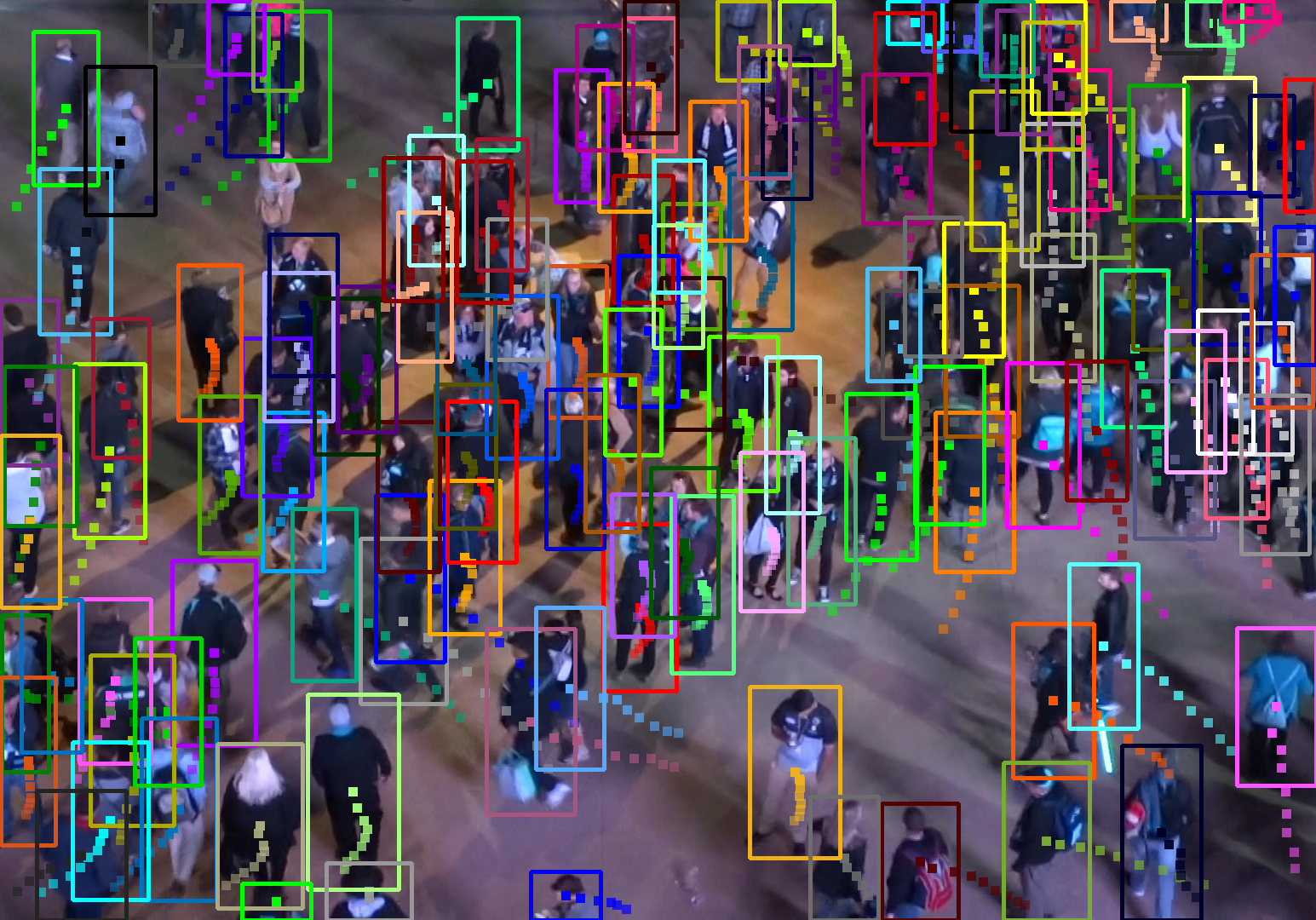
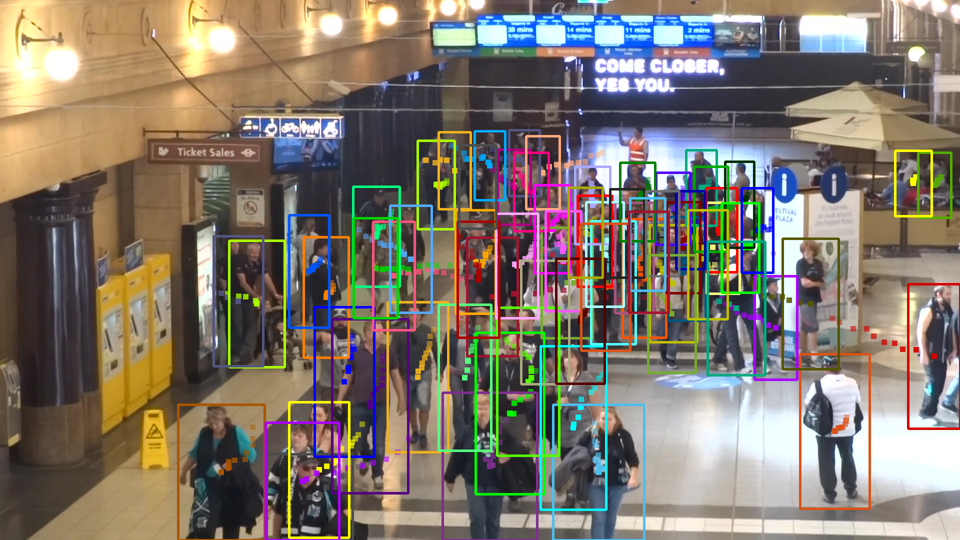
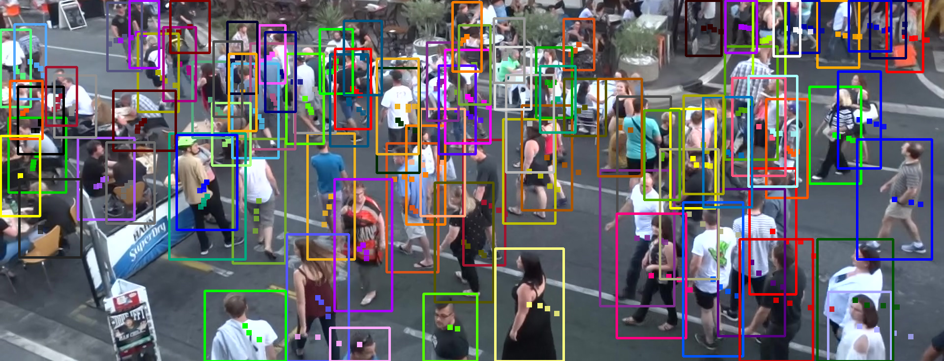
4.6 Qualitative Visualizations in Crowded Scenes
We report in Fig. 6 the qualitative results from some crowded MOT20 sequences, to demonstrate the detection and tracking abilities of TransCenterĩn the context of crowded scenes. Concretely, we show in Fig. 6 the predicted center trajectories and the corresponding object sizes. Fig. 6(a) is extracted from MOT20-04, Fig. 6(b) from MOT20-07 and Fig. 6(c) from MOT20-06. We observe that TransCenter manages to keep high recall, even in the context of drastic mutual occlusions, and reliably associate detections across time. To summarize, TransCenter exhibits outstanding results on both MOT17 and MOT20 datasets for both public and private detections, and for both with or without extra training data, which indicates that multiple-object center tracking using transformers equipped with dense image-related queries is a promising research direction.
5 Conclusion
In this paper, we introduce TransCenter, a powerful and efficient transformer-based architecture with dense image-related representations for multiple-object tracking. In TransCenter, we propose the use of dense pixel-level multi-scale detection queries and sparse tracking queries. They are produced with carefully-designed QLN and interacting in TransCenter Decoder with image features. Under the same training conditions, TransCenter outperforms its competitors in MOT17 and by a large margin in very crowded scenes in MOT20. It even exhibits better performance than some methods trained with much more data. More importantly, TransCenter maintains a reasonably high efficiency while exhibiting a state-of-the-art performance, thanks to its careful designs proven by a thorough ablation.
Supplementary Material
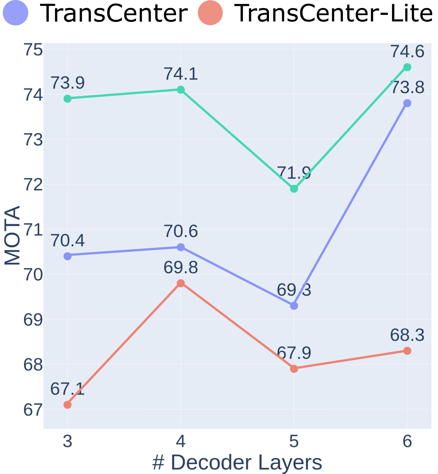
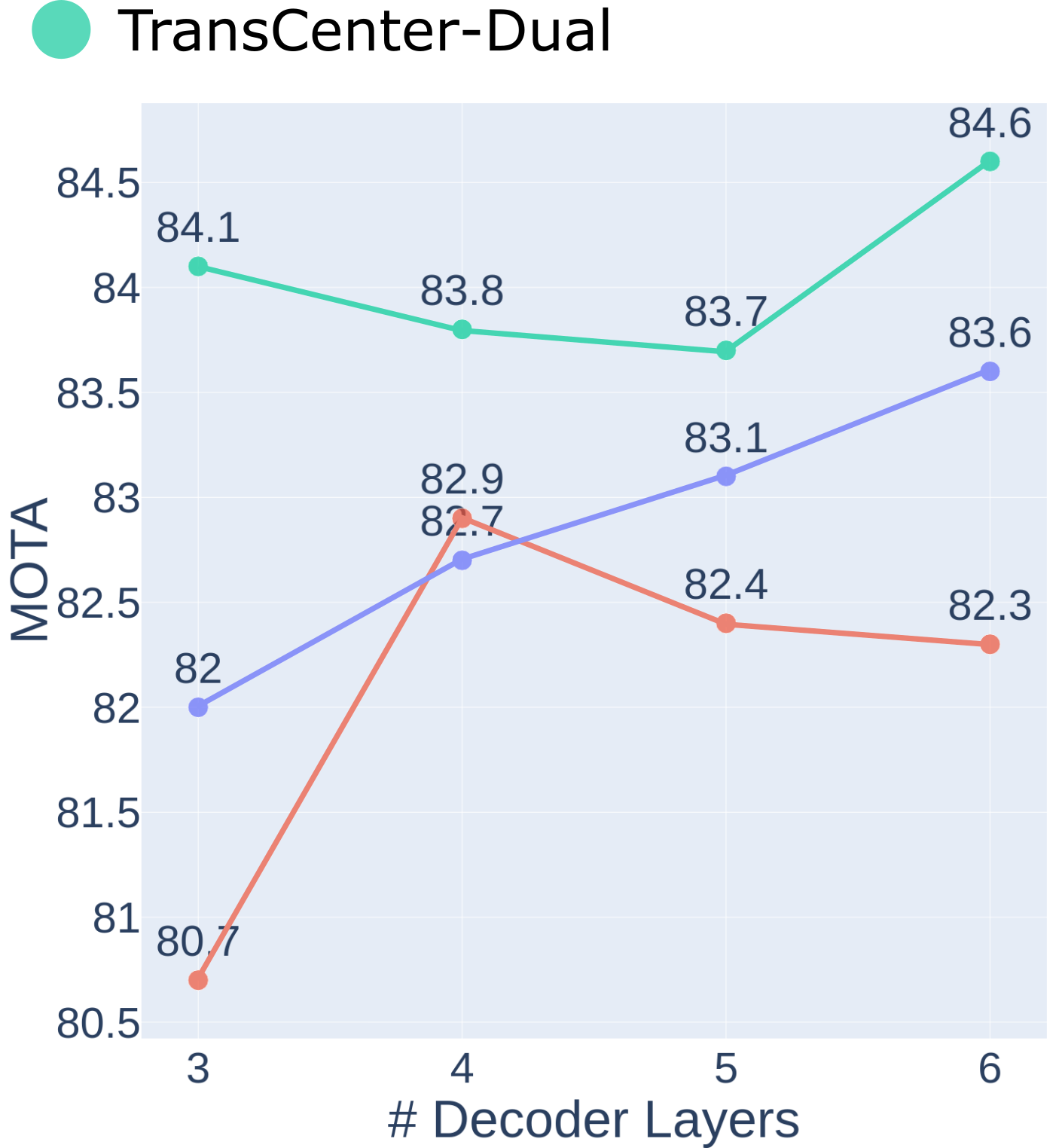
Appendix A Number of Decoder Layers
We ablate in Fig. 7 the number of decoder layers in TransCenter, TransCenter-Lite, and TransCenter-Dual. Precisely, we search the best number of decoder layers within the range of For TransCenter, TransCenter-Dual, we find that having six layers of decoder gets the best results in terms of MOTA both in MOT17 and MOT20 while with four layers in TransCenter-Lite.
Appendix B Qualitative Results and Visualizations
In this section, we qualitatively visualize the center heatmap responses (Sec. B.1), the detection queries (Sec. B.2) and the tracking queries (Sec. B.3) of TransCenter.
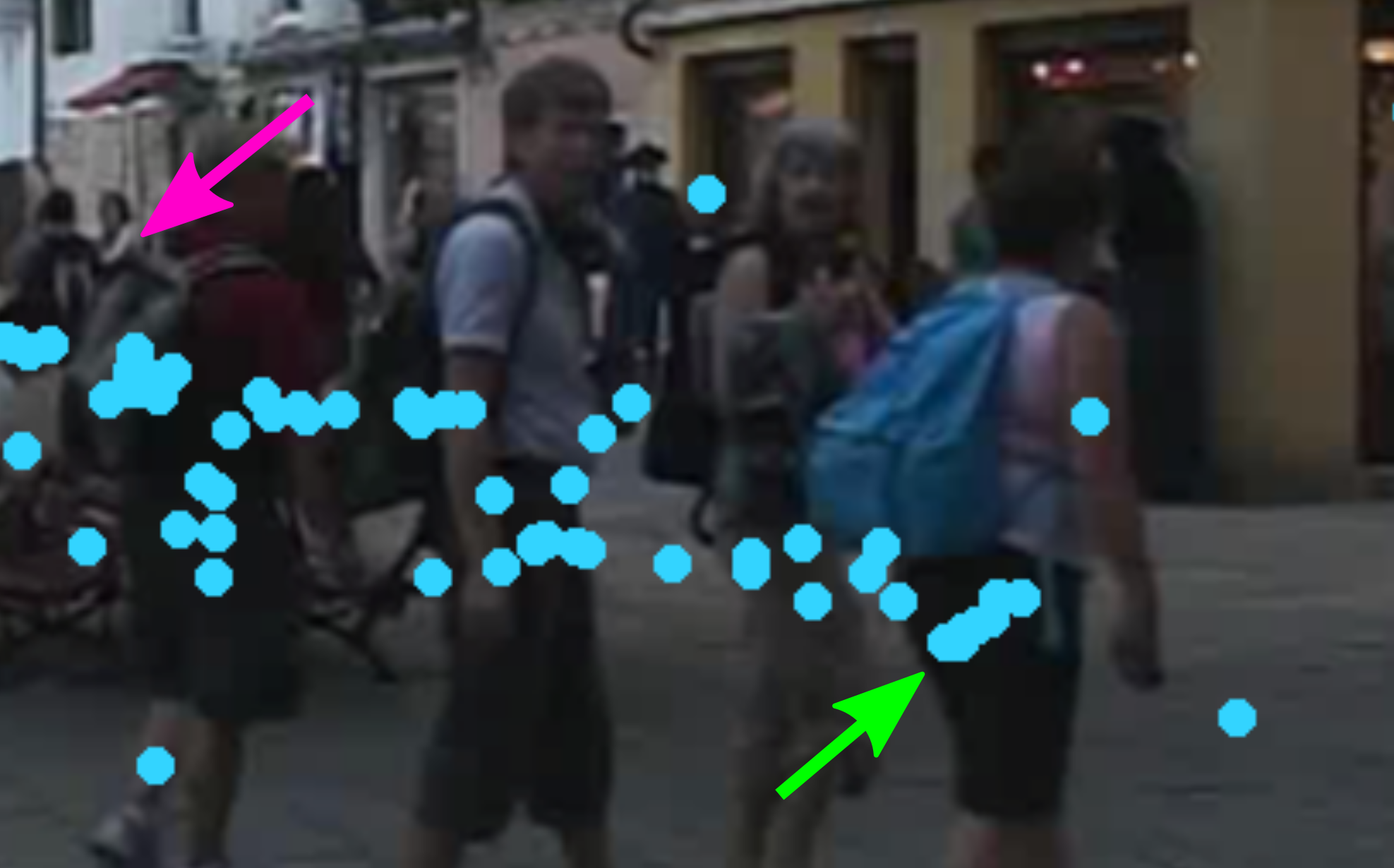
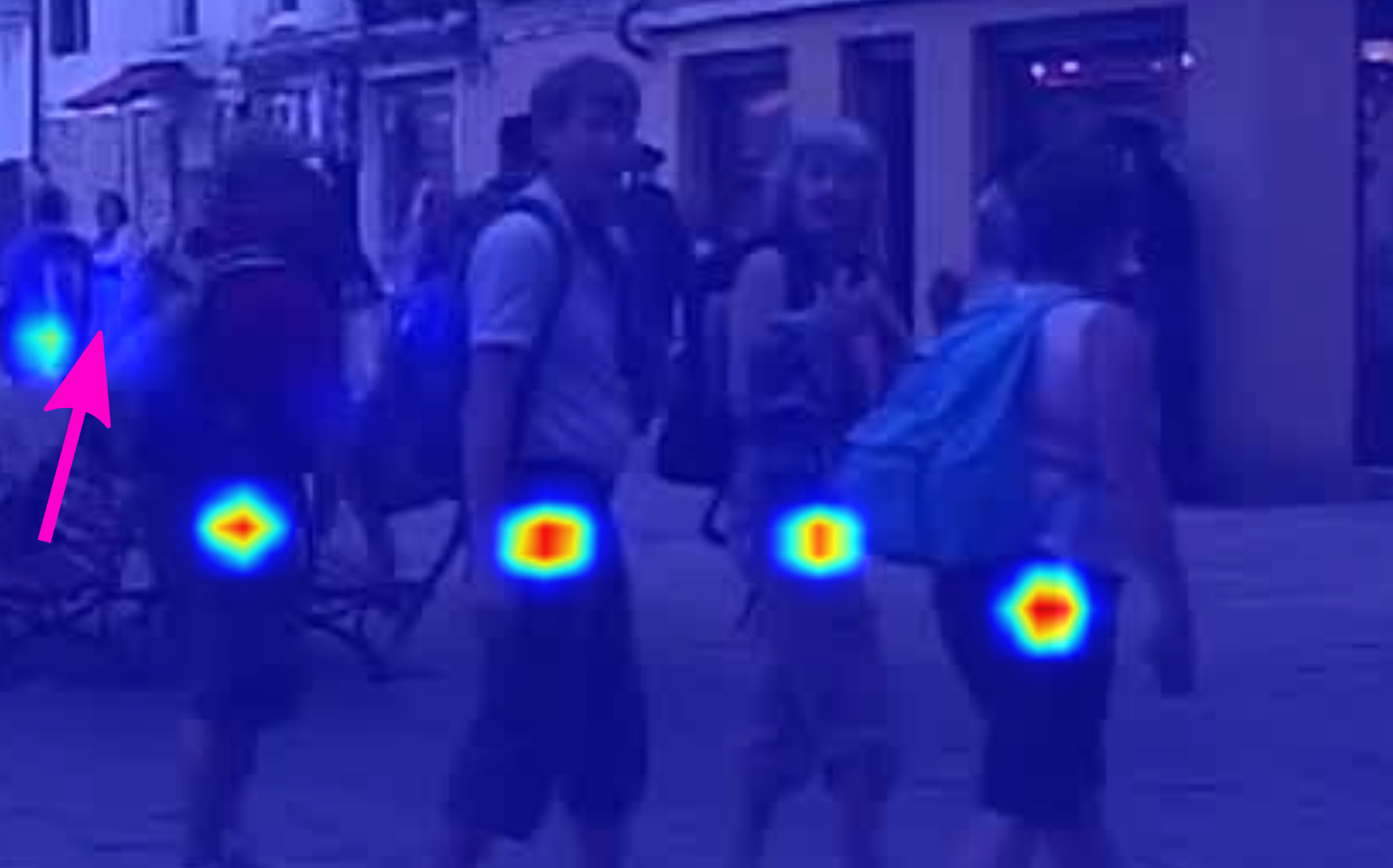
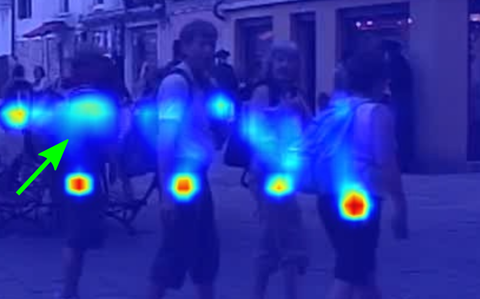
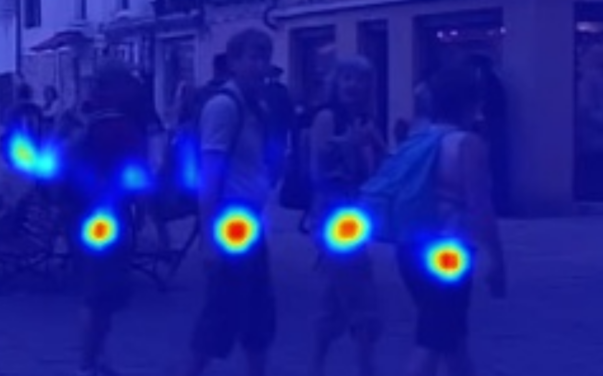
B.1 Center Heatmap Response
We qualitatively visualize and compare our center heatmap response in Fig. 8(d) with other two center heatmap-based MOT methods [94, 89] in Fig. 8(c) and Fig. 8(b) as well as the box centers predicted from sparse queries from one concurrent transformer-based MOT method [65] in Fig. 8(a).
Two concurrent transformer-based MOT methods [65, 45] both use sparse queries, leading to miss detections (pink arrow), that are heavily overlapped, possibly leading to false detections (green arrow). Previous center-based MOT methods [94, 89] suffer from the same problems because the centers are estimated locally. TransCenter is designed to mitigate these two adverse effects by using dense (pixel-level) image-related detection queries producing a dense representation to enable heatmap-based inference and exploiting the attention mechanisms to introduce co-dependency among center predictions.
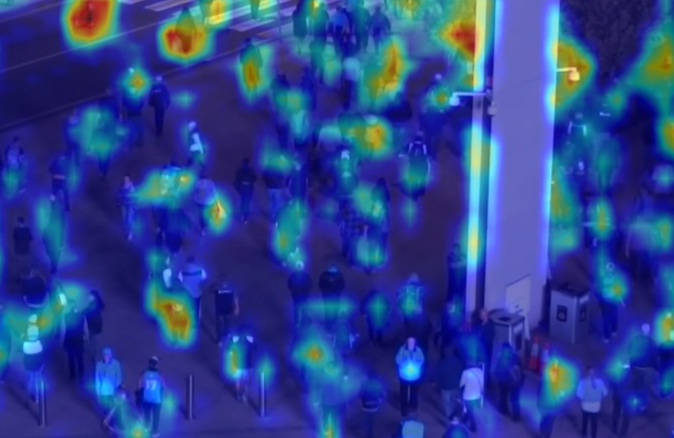
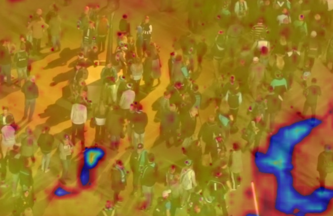
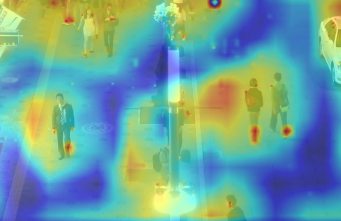
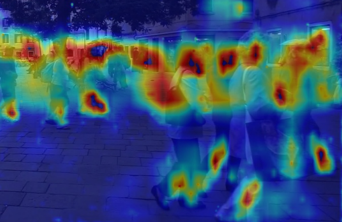
B.2 Detection-Query Visualization
We visualize in Fig. 9 the detection queries from TransCenter using the gradient-weighted class activation mapping, as described in [60]. The intuition is that we can consider the center heatmap prediction as a 2D classification task, similar to image segmentation. The center heatmap response is class-specific where the class is binary with ”person” or ”background”. Precisely, we calculate the gradient from the center heatmap w.r.t. the detection queries. The gradient is averaged over the image height and width. It is served as weights for the dense detection queries (), producing weighted activations after multiplication. Since our dense detection queries are multi-scale, we re-scale the activations to the input image size and take the average of pixel values from all scales. The activation is plotted above the input image to show the link between their activated values and the object positions. For the visualization purpose, negative values are removed (by a ReLU activation function) and a normalization process by the maximum activation value is performed. From the visualizations, we can see that the detection queries tend to focus on areas where pedestrians are gathered. This is intuitive since the dense detection queries are used to find objects in a given scene.
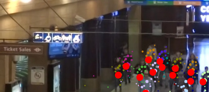
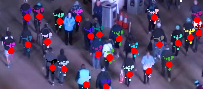
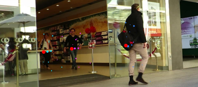
B.3 Tracking-Query Visualization
Differently, the tracking queries in TransCenter are sparse and thus cannot be plotted directly to an image like the detection queries. Therefore, we visualize them differently: Recall that and interact in TDCA (see Sec. 3.2 in the main paper) for the tracking inside TransCenter Decoder, where we sample object features from the input . The sampling locations are obtained by displacing the input reference points (normalized object center positions at the previous frame) with sampling offsets (several offsets per reference point) learned from . Moreover, the sampled features are weighted by the attention weights learned from . Based on this mechanism, we visualize the tracking queries by looking at the sampling locations (displaced reference points) in the image . Concretely, we show in Fig. 10 the reference points (track positions at , is set to 5 for better visualization) as red dots. The sampling locations are shown in circles with different colors referring to different object identities. Their radius is proportional to their attention weight (i.e. a bigger circle means a higher attention weight) and we filter out sampling locations with weights lower than a threshold (e.g. 0.2) for better visualizations. From Fig. 10, interestingly, we can see that the sampling locations are the surrounding of the corresponding objects and the weights and the attention weights get smaller when the locations get further from the object. This indicates qualitatively that the tracking queries from the previous time step are searching objects at in their neighborhood.
Acknowledgments
Xavier Alameda-Pineda acknowledges funding from the ANR ML3RI project (ANR-19-CE33-0008-01) and the H2020 SPRING project (under GA #871245).
References
- [1] Nathanael L Baisa. Online multi-object visual tracking using a gm-phd filter with deep appearance learning. In FUSION, pages 1–8. IEEE, 2019.
- [2] Yutong Ban, Xavier Alameda-Pineda, Laurent Girin, and Radu Horaud. Variational bayesian inference for audio-visual tracking of multiple speakers. TPAMI, 2019.
- [3] Yutong Ban, Sileye Ba, Xavier Alameda-Pineda, and Radu Horaud. Tracking multiple persons based on a variational bayesian model. In ECCV, pages 52–67. Springer, 2016.
- [4] Philipp Bergmann, Tim Meinhardt, and Laura Leal-Taixe. Tracking without bells and whistles. In ICCV, pages 941–951, 2019.
- [5] Keni Bernardin and Rainer Stiefelhagen. Evaluating multiple object tracking performance: the clear mot metrics. EURASIP Journal on Image and Video Processing, 2008:1–10, 2008.
- [6] Alex Bewley, Zongyuan Ge, Lionel Ott, Fabio Ramos, and Ben Upcroft. Simple online and realtime tracking. In IEEE international Conference on Image Processing (ICIP), pages 3464–3468. IEEE, 2016.
- [7] Guillem Brasó and Laura Leal-Taixé. Learning a neural solver for multiple object tracking. In CVPR, pages 5247–6257. IEEE, 2020.
- [8] Nicolas Carion, Francisco Massa, Gabriel Synnaeve, Nicolas Usunier, Alexander Kirillov, and Sergey Zagoruyko. End-to-end object detection with transformers. In ECCV, pages 213–229. Springer, 2020.
- [9] Long Chen, Haizhou Ai, Zijie Zhuang, and Chong Shang. Real-time multiple people tracking with deeply learned candidate selection and person re-identification. In ICME, pages 1–6. IEEE, 2018.
- [10] Jifeng Dai, Haozhi Qi, Yuwen Xiong, Yi Li, Guodong Zhang, Han Hu, and Yichen Wei. Deformable convolutional networks. In ICCV, pages 764–773. IEEE, 2017.
- [11] P. Dendorfer, H. Rezatofighi, A. Milan, J. Shi, D. Cremers, I. Reid, S. Roth, K. Schindler, and L. Leal-Taixé. Mot20: A benchmark for multi object tracking in crowded scenes. In arXiv:2003.09003[cs], 2020.
- [12] Piotr Dollár, Christian Wojek, Bernt Schiele, and Pietro Perona. Pedestrian detection: An evaluation of the state of the art. TPAMI, 34:743–761, 2011.
- [13] Alexey Dosovitskiy, Lucas Beyer, Alexander Kolesnikov, Dirk Weissenborn, Xiaohua Zhai, Thomas Unterthiner, Mostafa Dehghani, Matthias Minderer, Georg Heigold, Sylvain Gelly, et al. An image is worth 16x16 words: Transformers for image recognition at scale. arXiv:2010.11929, 2020.
- [14] A. Ess, B. Leibe, K. Schindler, , and L. van Gool. A mobile vision system for robust multi-person tracking. In CVPR, pages 1–8. IEEE, 2008.
- [15] Chuang Gan, Deng Huang, Peihao Chen, Joshua B Tenenbaum, and Antonio Torralba. Foley music: Learning to generate music from videos. ECCV, pages 758–775, 2020.
- [16] Chuang Gan, Deng Huang, Hang Zhao, Joshua B Tenenbaum, and Antonio Torralba. Music gesture for visual sound separation. In CVPR, pages 10478–10487. IEEE, 2020.
- [17] Chuang Gan, Hang Zhao, Peihao Chen, David Cox, and Antonio Torralba. Self-supervised moving vehicle tracking with stereo sound. In ICCV, pages 7053–7062. IEEE, 2019.
- [18] Zheng Ge, Songtao Liu, Feng Wang, Zeming Li, and Jian Sun. Yolox: Exceeding yolo series in 2021. arXiv preprint arXiv:2107.08430, 2021.
- [19] Andreas Geiger, Philip Lenz, and Raquel Urtasun. Are we ready for autonomous driving? the kitti vision benchmark suite. In CVPR, pages 3354–3361, 2012.
- [20] Nicolas Franco Gonzalez, Andres Ospina, and Philippe Calvez. Smat: Smart multiple affinity metrics for multiple object tracking. In International Conference on Image Analysis and Recognition (ICIAR), pages 48–62, 2020.
- [21] Song Guo, Jingya Wang, Xinchao Wang, and Dacheng Tao. Online multiple object tracking with cross-task synergy. In CVPR, pages 8136–8145, 2021.
- [22] Shoudong Han, Piao Huang, Hongwei Wang, En Yu, Donghaisheng Liu, Xiaofeng Pan, and Jun Zhao. Mat: Motion-aware multi-object tracking. arXiv:2009.04794, 2020.
- [23] Jiawei He, Zehao Huang, Naiyan Wang, and Zhaoxiang Zhang. Learnable graph matching: Incorporating graph partitioning with deep feature learning for multiple object tracking. In IEEE Conference on Computer Vision and Pattern Recognition (CVPR), pages 5299–5309, 2021.
- [24] Kaiming He, Xiangyu Zhang, Shaoqing Ren, and Jian Sun. Deep residual learning for image recognition. In CVPR, pages 770–778. IEEE, 2016.
- [25] Shuting He, Hao Luo, Pichao Wang, Fan Wang, Hao Li, and Wei Jiang. Transreid: Transformer-based object re-identification. arXiv:2102.04378, 2021.
- [26] Andrea Hornakova, Roberto Henschel, Bodo Rosenhahn, and Paul Swoboda. Lifted disjoint paths with application in multiple object tracking. In ICML, pages 4364–4375. PMLR, 2020.
- [27] Tak-Wai Hui, Xiaoou Tang, and Chen Change Loy. Liteflownet: A lightweight convolutional neural network for optical flow estimation. In CVPR, pages 8981–8989. IEEE, 2018.
- [28] Deng Jia, Dong Wei, Sochera Richard, Li Li-Jia, Li Kai, and Fei-Fei Li. Imagenet: A large-scale hierarchical image database. In CVPR. IEEE, 2009.
- [29] Yifan Jiang, Shiyu Chang, and Zhangyang Wang. Transgan: Two transformers can make one strong gan. arXiv:2102.07074, 2021.
- [30] Shyamgopal Karthik, Ameya Prabhu, and Vineet Gandhi. Simple unsupervised multi-object tracking. arXiv:2006.02609, 2020.
- [31] Hasith Karunasekera, Han Wang, and Handuo Zhang. Gnn3dmot: Graph neural network for 3d multi-object tracking with 2d-3d multi-feature learning. In IEEE Access, pages 104423–104434. IEEE, 2019.
- [32] Margret Keuper, Siyu Tang, Yu Zhongjie, Bjoern Andres, Thomas Brox, and Bernt Schiele. A multi-cut formulation for joint segmentation and tracking of multiple objects. arXiv:1607.06317, 2016.
- [33] Chanho Kim, Fuxin Li, Mazen Alotaibi, and James M Rehg. Discriminative appearance modeling with multi-track pooling for real-time multi-object tracking. In CVPR, pages 9553–9562. IEEE, 2021.
- [34] Harold W. Kuhn and Bryn Yaw. The hungarian method for the assignment problem. In Naval Res. Logist. Quart, pages 83–97. IEEE, 1955.
- [35] Hei Law and Jia Deng. Cornernet: Detecting objects as paired keypoints. In ECCV, pages 734–750. IEEE, 2018.
- [36] Wei Li, Rui Zhao, Tong Xiao, and Xiaogang Wang. Deepreid: Deep filter pairing neural network for person re-identification. In CVPR, pages 152–159. IEEE, 2014.
- [37] Yuan Li, Chang Huang, and Ram Nevatia. Learning to associate: Hybridboosted multi-target tracker for crowded scene. In CVPR, pages 2953–2960. IEEE, 2009.
- [38] Chao Liang, Zhipeng Zhang, Yi Lu, Xue Zhou, Bing Li, Xiyong Ye, and Jianxiao Zou. Rethinking the competition between detection and reid in multi-object tracking. arXiv:2010.12138, 2020.
- [39] Matthieu Lin, Chuming Li, Xingyuan Bu, Ming Sun, Chen Lin, Junjie Yan, Wanli Ouyang, and Zhidong Deng. Detr for crowd pedestrian detection. arXiv:2012.06785, 2020.
- [40] Tsung-Yi Lin, Michael Maire, Serge Belongie, James Hays, Pietro Perona, Deva Ramanan, Piotr Dollár, and C Lawrence Zitnick. Microsoft coco: Common objects in context. In ECCV, pages 740–755. Springer, 2014.
- [41] Xiaoyu Lin, Laurent Girin, and Xavier Alameda-Pineda. Unsupervised multiple-object tracking with a dynamical variational autoencoder. In arXiv:2202.09315, 2022.
- [42] Qiankun Liu, Qi Chu, Bin Liu, and Nenghai Yu. Gsm: Graph similarity model for multi-object tracking. In International Joint Conference on Artificial Intelligence (IJCAI), pages 530–536. International Joint Conferences on Artificial Intelligence Organization, 2020.
- [43] Yuanpei Liu, Junbo Yin, Dajiang Yu, Sanyuan Zhao, and Jianbing Shen. Multiple people tracking with articulation detection and stitching strategy. Neurocomputing, 386:18–29, 2020.
- [44] Ilya Loshchilov and Frank Hutter. Decoupled weight decay regularization. In ICLR, 2017.
- [45] Tim Meinhardt, Alexander Kirillov, Laura Leal-Taixe, and Christoph Feichtenhofer. Trackformer: Multi-object tracking with transformers. arXiv:2101.02702, 2021.
- [46] Anton Milan, Laura Leal-Taixé, Ian D. Reid, Stefan Roth, and Konrad Schindler. MOT16: A benchmark for multi-object tracking. arXiv:1603.00831 [cs], 2016.
- [47] Anton Milan, S Hamid Rezatofighi, Anthony Dick, Ian Reid, and Konrad Schindler. Online multi-target tracking using recurrent neural networks. In AAAI, 2017.
- [48] Jiangmiao Pang, Linlu Qiu, Xia Li, Haofeng Chen, Qi Li, Trevor Darrell, and Fisher Yu. Quasi-dense similarity learning for multiple object tracking. In CVPR, pages 164–173. IEEE, 2021.
- [49] Ioannis Papakis, Abhijit Sarkar, and Anuj Karpatne. Gcnnmatch: Graph convolutional neural networks for multi-object tracking via sinkhorn normalization. arXiv:2010.00067, 2020.
- [50] Jinlong Peng, Changan Wang, Fangbin Wan, Yang Wu, Yabiao Wang, Ying Tai, Chengjie Wang, Jilin Li, Feiyue Huang, and Yanwei Fu. Chained-tracker: Chaining paired attentive regression results for end-to-end joint multiple-object detection and tracking. In ECCV, pages 145–161. Springer, 2020.
- [51] Dollár Piotr, Wojek Christian, Schiele Bernt, and Perona Pietro. Pedestrian detection: A benchmark. In CVPR. IEEE, 2009.
- [52] Akshay Rangesh, Pranav Maheshwari, Mez Gebre, Siddhesh Mhatre, Vahid Ramezani, and Mohan M. Trivedi. Trackmpnn: A message passing graph neural architecture for multi-object tracking. arXiv:2010.12138, 2021.
- [53] Joseph Redmon, Santosh Divvala, Ross Girshick, and Ali Farhadi. You only look once: Unified, real-time object detection. In CVPR, pages 779–788. IEEE, 2016.
- [54] Shaoqing Ren, Kaiming He, Ross Girshick, and Jian Sun. Faster r-cnn: Towards real-time object detection with region proposal networks. NeurIPS, pages 91–99, 2015.
- [55] Seyed Hamid Rezatofighi, Anton Milan, Zhen Zhang, Qinfeng Shi, Anthony Dick, and Ian Reid. Joint probabilistic data association revisited. In ICCV, pages 3047–3055. IEEE, 2015.
- [56] Ergys Ristani, Francesco Solera, Roger Zou, Rita Cucchiara, and Carlo Tomasi. Performance measures and a data set for multi-target, multi-camera tracking. In ECCV, pages 17–35. Springer, 2016.
- [57] Amir Sadeghian, Alexandre Alahi, and Silvio Savarese. Tracking the untrackable: Learning to track multiple cues with long-term dependencies. In ICCV, pages 300–311. IEEE, 2017.
- [58] Fatemeh Saleh, Sadegh Aliakbarian, Hamid Rezatofighi, Mathieu Salzmann, and Stephen Gould. Probabilistic tracklet scoring and inpainting for multiple object tracking. In CVPR, pages 14329–14339. IEEE, 2021.
- [59] Manen Santiago, Gygli Michael, Dai Dengxin, and Van Gool Luc. Pathtrack: Fast trajectory annotation with path supervision. In ICCV, pages 290–299. IEEE, 2017.
- [60] Ramprasaath R. Selvaraju, Michael Cogswell, Abhishek Das, Ramakrishna Vedantam, Devi Parikh, and Dhruv Batra. Grad-cam: Visual explanations from deep networks via gradient-based localization. In IJCV, pages 1573–1405. Springer, 2019.
- [61] Chaobing Shan, Chunbo Wei, Bing Deng, Jianqiang Huang, Xian-Sheng Hua, Xiaoliang Cheng, and Kewei Liang. Tracklets predicting based adaptive graph tracking, 2020.
- [62] Shuai Shao, Zijian Zhao, Boxun Li, Tete Xiao, Gang Yu, Xiangyu Zhang, and Jian Sun. Crowdhuman: A benchmark for detecting human in a crowd. arXiv:1805.00123, 2018.
- [63] Jianbing Shen, Dajiang Yu, Leyao Deng, and Xingping Dong. Fast online tracking with detection refinement. TITS, 19(1):162–173, 2017.
- [64] Bing Shuai, Andrew Berneshawi, Xinyu Li, Davide Modolo, and Joseph Tighe. Siammot: Siamese multi-object tracking. In CVPR, pages 12372–12382. IEEE, 2021.
- [65] Peize Sun, Yi Jiang, Rufeng Zhang, Enze Xie, Jinkun Cao, Xinting Hu, Tao Kong, Zehuan Yuan, Changhu Wang, and Ping Luo. Transtrack: Multiple-object tracking with transformer. In arXiv:2012.15460, 2020.
- [66] Siyu Tang, Bjoern Andres, Miykhaylo Andriluka, and Bernt Schiele. Subgraph decomposition for multi-target tracking. In CVPR, pages 5033–5041. IEEE, 2015.
- [67] Siyu Tang, Bjoern Andres, Mykhaylo Andriluka, and Bernt Schiele. Multi-person tracking by multicut and deep matching. In ECCV, pages 100–111. Springer, 2016.
- [68] Siyu Tang, Mykhaylo Andriluka, Bjoern Andres, and Bernt Schiele. Multiple people tracking by lifted multicut and person re-identification. In CVPR, pages 3539–3548. IEEE, 2017.
- [69] Phillip Thomas, Lars Pandikow, Alex Kim, Michael Stanley, and James Grieve. Open synthetic dataset for improving cyclist detection. In https://paralleldomain.com/open-datasets/bicycle-detection, 2021.
- [70] Pavel Tokmakov, Jie Li, Wolfram Burgard, and Adrien Gaidon. Learning to track with object permanence. In ICCV, pages 10860–10869. IEEE, 2021.
- [71] Ashish Vaswani, Noam Shazeer, Niki Parmar, Jakob Uszkoreit, Llion Jones, Aidan N Gomez, Lukasz Kaiser, and Illia Polosukhin. Attention is all you need. In NeurIPS, pages 5998–6008, 2017.
- [72] Qiang Wang, Yun Zheng, Pan Pan, and Yinghui Xu. Multiple object tracking with correlation learning. In CVPR, pages 3876–3886. IEEE, 2021.
- [73] Wenhai Wang, Enze Xie, Xiang Li, Deng-Ping Fan, Kaitao Song, Ding Liang, Tong Lu, Ping Luo, and Ling Shao. Pvt v2: Improved baselines with pyramid vision transformer. In Computational Visual Media (CVM), pages 1–10, 2022.
- [74] Yongxin Wang, Kris Kitani, and Xinshuo Weng. Joint object detection and multi-object tracking with graph neural networks. In ICRA. IEEE, 2021.
- [75] Xinshuo Weng, Jianren Wang, David Held, and Kris Kitani. 3d multi-object tracking: A baseline and new evaluation metrics. arXiv:1907.03961, 2020.
- [76] Xinshuo Weng, Yongxin Wang, Yunze Man, and Kris M Kitani. Gnn3dmot: Graph neural network for 3d multi-object tracking with 2d-3d multi-feature learning. In CVPR, pages 6499–6508. IEEE, 2020.
- [77] Xinshuo Weng, Ye Yuan, and Kris Kitani. Joint 3d tracking and forecasting with graph neural network and diversity sampling. arXiv:2003.07847, 2020.
- [78] Jialian Wu, Jiale Cao, Liangchen Song, Yu Wang, Ming Yang, and Junsong Yuan. Track to detect and segment: An online multi-object tracker. In CVPR, pages 12352–12361. IEEE, 2021.
- [79] Yu Xiang, Alexandre Alahi, and Silvio Savarese. Learning to track: Online multi-object tracking by decision making. In ICCV, pages 4705–4713. IEEE, 2015.
- [80] Tong Xiao, Shuang Li, Bochao Wang, Liang Lin, and Xiaogang Wang. End-to-end deep learning for person search. arXiv:1604.01850, 2016.
- [81] Yihong Xu, Aljosa Osep, Yutong Ban, Radu Horaud, Laura Leal-Taixé, and Xavier Alameda-Pineda. How to train your deep multi-object tracker. In CVPR, pages 6787–6796. IEEE, 2020.
- [82] Fuzhi Yang, Huan Yang, Jianlong Fu, Hongtao Lu, and Baining Guo. Learning texture transformer network for image super-resolution. In CVPR, pages 5791–5800. IEEE, 2020.
- [83] Junbo Yin, Wenguan Wang, Qinghao Meng, Ruigang Yang, and Jianbing Shen. A unified object motion and affinity model for online multi-object tracking. In CVPR, pages 6768–6777. IEEE, 2020.
- [84] En Yu, Zhuoling Li, Shoudong Han, and Hongwei Wang. Relationtrack: Relation-aware multiple object tracking with decoupled representation. arXiv:2105.04322, 2021.
- [85] Fangao Zeng, Bin Dong, Tiancai Wang, Xiangyu Zhang, and Yichen Wei. End-to-end multiple-object tracking with transformer. In arXiv:2105.03247, 2021.
- [86] Shanshan Zhang, Rodrigo Benenson, and Bernt Schiele. Citypersons: A diverse dataset for pedestrian detection. In CVPR, pages 3213–3221. IEEE, 2017.
- [87] Yang Zhang, Hao Sheng, Yubin Wu, Shuai Wang, Wei Ke, and Zhang Xiong. Multiplex labeling graph for near-online tracking in crowded scenes. IEEE Internet of Things Journal, pages 7892–7902, 2020.
- [88] Yifu Zhang, Peize Sun, Yi Jiang, Dongdong Yu, Zehuan Yuan, Ping Luo, Wenyu Liu, and Xinggang Wang. Bytetrack: Multi-object tracking by associating every detection box. In arXiv:2110.06864, 2021.
- [89] Yifu Zhang, Chunyu Wang, Xinggang Wang, Wenjun Zeng, and Wenyu Liu. Fairmot: On the fairness of detection and re-identification in multiple object tracking. In arXiv:2004.01888, 2020.
- [90] Zhi Zhang, Tong He, Hang Zhang, Zhongyue Zhang, Junyuan Xie, and Mu Li. Bag of freebies for training object detection neural networks. arXiv preprint arXiv:1902.04103, 2019.
- [91] Liang Zheng, Liyue Shen, Lu Tian, Shengjin Wang, Jingdong Wang, and Qi Tian. Scalable person re-identification: A benchmark. In ICCV. IEEE, 2015.
- [92] Liang Zheng, Hengheng Zhang, Shaoyan Sun, Manmohan Chandraker, Yi Yang, and Qi Tian. Person re-identification in the wild. In CVPR, pages 1367–1376. IEEE, 2017.
- [93] Linyu Zheng, Ming Tang, Yingying Chen, Guibo Zhu, Jinqiao Wang, and Hanqing Lu. Improving multiple object tracking with single object tracking. In CVPR, pages 2453–2462. IEEE, 2021.
- [94] Xingyi Zhou, Vladlen Koltun, and Philipp Krähenbühl. Tracking objects as points. In ECCV, pages 474–490. Springer, 2020.
- [95] Xingyi Zhou, Dequan Wang, and Philipp Krähenbühl. Objects as points. arXiv:1904.07850, 2019.
- [96] Tianyu Zhu, Markus Hiller, Mahsa Ehsanpour, Rongkai Ma, Tom Drummond, and Hamid Rezatofighi. Looking beyond two frames: End-to-end multi-object tracking using spatial and temporal transformers. arXiv preprint arXiv:2103.14829, 2021.
- [97] Xizhou Zhu, Weijie Su, Lewei Lu, Bin Li, Xiaogang Wang, and Jifeng Dai. Deformable detr: Deformable transformers for end-to-end object detection. arXiv:2010.04159, 2020.