Constraining Theories of Gravity by GINGER experiment

Abstract

The debate on gravity theories to extend or modify General Relativity is very active today because of the issues related to ultra-violet and infra-red behavior of Einstein’s theory. In the first case, we have to address the Quantum Gravity problem. In the latter, dark matter and dark energy, governing the large scale structure and the cosmological evolution, seem to escape from any final fundamental theory and detection. The state of art is that, up to now, no final theory, capable of explaining gravitational interaction at any scale, has been formulated. In this perspective, many research efforts are devoted to test theories of gravity by space-based experiments. Here we propose straightforward tests by the GINGER experiment, which, being Earth based, requires little modeling of external perturbation, allowing a thorough analysis of the systematics, crucial for experiments where sensitivity breakthrough is required. Specifically, we want to show that it is possible to constrain parameters of gravity theories, like scalar-tensor or Horava-Lifshitz gravity, by considering their post-Newtonian limits matched with experimental data. In particular, we use the Lense-Thirring measurements provided by GINGER to find out relations among the parameters of theories and finally compare the results with those provided by LARES and Gravity Probe-B satellites.

Pacs   04.50.Kd; 04.80.Cc; 91.10.Op.

1 Introduction

General Relativity (GR) is one of the cornerstones of modern Physics predicting the behavior of gravitational field from very large astrophysical scales up to local scales. For instance, it provides corrections to the path of planets orbiting around stars, which undergo a perihelion precession which cannot be theoretically obtained by Newtonian gravity. Moreover, in the last few years, the gravitational waves detection Abbott:2016blz ; TheLIGOScientific:2017qsa ; Abbott:2017vtc ; Monitor:2017mdv ; Abbott:2017oio and the confirmation of the existence of black holes Akiyama:2019cqa further corroborated the validity of the Einstein geometric view of gravitational interaction. The theory satisfactorily explains most of the cosmic evolution, starting from the very early up to the present epoch giving rise to the so called Cosmological Standard Model Weinberg . For these reasons, nowadays GR is the best accepted theory describing gravity.

Nevertheless, though it fits a large amount of observational data, it suffers many problems at very large and very small scales. Several shortcomings arise in the attempt to coherently describe the large-scale structure and cosmology. In particular, recent observations suggest that the universe is undergoing an accelerated expansion in the late epoch. The current explanation for this issue is that the expansion should be driven by a cosmological constant $\Lambda$ acting at large scales or some form of dark energy which allows the evolution of cosmological constant from early to present epochs. According to the observations, dark energy represents almost 70$\%$ of the whole matter-energy content of the universe, but a final explanation of its fundamental nature is still missing.

On the other hand, the velocity of stars and gas clouds orbiting around galaxies led to introduce an unknown form of dark matter Sahni:2004ai ; Catena:2009mf ; Navarro:1995iw ; Bertone:2004pz . Its existence was firstly inferred by the observations of the galaxy rotation curves. Astrometric data suggest that dark matter in the universe is of the order of 25 - 30 $\%$ of the total amount of cosmic matter-energy leaving very little room for the observed ordinary baryonic matter. Also in the case of dark matter, there is no final evidence, at fundamental quantum level, also if its cumulative effects are present at astrophysical scales.

Dark energy and dark matter constitute the most striking shortcomings of Cosmological Standard Model if no final signature of their existence is revealed at fundamental level, despite of the several models proposed to explain them.

Furthermore, at ultraviolet scales, GR cannot be dealt under the standard formalism of Quantum Field Theory. The reason is because space and time cannot be simply considered as quantum variables. Several approaches are under scrutiny like the canonical formalism, started from the early works by Arnowitt, Deser, and Misner Thiemann:2007zz ; Arnowitt:1960es ; Misner:1969ae ; Arnowitt:1962hi ; Bajardi:2020fxh , the Quantum Field Theory formulation on curved spacetimes DeWitt:1975ys ; Padmanabhan:2003gd ; Calzetta:1986ey , the Superstring Theory String , the Supergravity VanNieuwenhuizen:1981ae and others, but none, up to now, can be considered the final, self-consistent formulation of Quantum Gravity Kiefer:2003ew .

However, under some assumptions, the semiclassical formulation (that is quantum fields formulated on curved ”classical” spaces) is giving rise to physically consistent results related, for example, to black holes Hawking:1974sw ; Bekenstein:1973ur ; Strominger:1996sh ; Gibbons:1976ue ; Banados:1992wn , to the inflationary universe Guth:1980zm ; Linde:1981mu ; Linde:1983gd ; Guth:1982ec ; Elizalde:2007zz and to other topics related to the behavior of gravitational field in strong regime. The paradigm is that, in the semiclassical limit, the gravitational action can be corrected with curvature invariants, scalar fields or other geometric invariants (like torsion) in order to represent the effective gravitational interaction Birrell ; Buchbinder:1992rb . As a result, the Hilbert-Einstein action of gravity results extended or modified giving the possibility to fix shortcomings of GR at infra-red and ultra-violet scales.

Essentially, these effective actions can be distinguished in two main categories: Extended Theories of Gravity Capozziello:2011et ; Wands:1993uu ; Crisostomi:2016czh ; Clifton:2011jh ; Nojiri:2006ri ; Bajardi:2020mdp ; Bajardi:2020osh ; Bajardi:2019zzs which improve the Hilbert-Einstein action involving higher-order curvature invariants or scalar fields, and Alternative Theories of Gravity, where some basic assumptions of GR are relaxed, as well as the torsionless connection, the metricity, or the universal validity of the Equivalence Principle Bajardi:2021tul ; Cai:2015emx ; Hammond:2002rm ; Sotiriou:2006qn ; BeltranJimenez:2019tjy ; Vitagliano:2010sr ; Frusciante:2015maa .

For instance, $f(R)$ gravity is a straightforward generalization of GR where a generic function of the Ricci curvature scalar $R$ is introduced relaxing the linearity in $R$. In this case, the field equations exhibit an effective energy-momentum tensor where further curvature components can play the role of dark energy and dark matter Capozziello:2002rd ; Sotiriou:2008rp ; DeFelice:2010aj ; Starobinsky:2007hu ; Nojiri:2006gh ; Capozziello:2006dj ; Cognola:2007zu . In particular, it is possible to show that such a curvature stress-energy tensor can be recast in a perfect fluid form where cosmological dynamics is ruled by the form of $f(R)$ function Capozziello:2018ddp .

It is possible to show that a conformal transformation provides the Hilbert-Einstein action minimally coupled to a scalar field $\phi$ related to the first derivative of $f(R)$ function Capozziello:2015hra ; Borowiec:2014wva ; Stabile:2013eha . This means that Extended Theories of Gravity can be recast in equivalent forms where GR is minimally coupled to one or more scalar fields depending on the involved degrees of freedom of gravitational action. Scalar fields are usually introduced to drive the cosmological inflation at early times and to mimicking dark energy behavior at late time of the universe expansion Capozziello:2002rd .

Other important classes of alternative theories of gravity are the so called Teleparallel Gravity Aldrovandi:2013wha , Symmetric Teleparallel Gravity Conroy:2017yln , Horava–Lifshitz gravity Horava:2009uw where the Lorentz–invariance turns out to be broken at fundamental level. In this perspective, it is important to point out that an apparatus like GINGER, for testing the Lorentz Invariance, is reliable as reported by J. Tasson and collaborators in the framework of the Extended Standard Model of Particles Jay2019 .

In general, modifying or extending the gravitational action, yields further degrees of freedom. Even the simplest extensions, like $f(R)$ gravity, lead to further gravitational waves modes Capozziello:2019klx and to fourth–order field equations, in the metric formalism, depending on the function $f(R)$.

Several phenomenological selection criteria aim to find out the form of $f(R)$ by best fitting observations. In Capozziello:2006ph ; Capozziello:2004us , for example, the theory is selected by means of galaxy rotation curves; in Santos:2007bs , cosmographic parameters are used in order to find the shape of action respecting the energy conditions. In Sotiriou:2008ya , actions providing bouncing universes are taken into account. From an astrophysical point of view, theories of gravity can be constrained according to the parameters of compact objects Astashenok or the multimessenger astronomy combining gravitational waves and electromagnetic signals Lombriser:2015sxa . Finally, space-based experiments like LARES and GravityProbe B satellites can give upper bounds on gravitational parameters (see e.g. Capozziello:2014mea ).

In principle, also ground-based experiments can be considered to constrain theories of gravity at some fundamental level. The main advantages of Earth based experiments are: $i)$ that they provide local responses, not averaged ones; $ii)$ they can be repeated in different locations; $iii)$ they do not require external perturbation modelling, nor independent gravity maps; $iv)$ synchronization and tuning are simpler than analogous space-based experiments; $v)$ moreover, the apparatuses can be periodically upgraded to refine the measurements.

In this paper, we propose to constrain theories of gravity exploiting the expected sensitivity on relativistic precessions of the GINGER (Gyroscopes IN General Relativity) experiment. In particular, we shall take into account metric theories, whose action includes curvature invariants and scalar fields. Another theory which we are going to test is the Horava–Lifshitz gravity which we shall describe below. In both cases, the scalar and vector potentials coming from the weak–field limit are derived. The aim is to constrain the free parameters of gravitational potentials by GINGER experimental data.

Specifically, GINGER is an Earth-based experiment suitable for measuring the Lense-Thirring and Geodesic precessions of the rotating Earth. The measurements of the rotation rate, by means of an array of ring lasers, provide the GR components of the gravito-magnetic field with a precision of at least 1% Tartaglia:2016jfo ; DiVirgilio:2020ior ; DiVirgilio:2017fuh ; Ruggiero:2015gha ; Bosi:2020dgg ; DiVirgilio:2021zmm . Recent results of its prototype GINGERino, at Gran Sasso Laboratories DiVirgilio:2021zmm , indicate that GINGER should be able to measure Geodesic and Lense-Thirring effects with an uncertainty of 1 part in $10^{4}$ and $10^{3}$, respectively, of their value calculated in the framework of GR. Therefore, we can falsify or constrain the parameter space of extended/modified theories of gravity by comparing their post–Newtonian (PN) and parameterized post–Newtonian (PPN) predictions to the corresponding GINGER measurements. The general purpose is to demonstrate that theories of gravity can be constrained not only by astrophysical and cosmological observations or space-satellites but also by terrestrial experiments that can be, in principle, more easily tuned and controlled Gurzadyan ; Gurzadyan1 .

The paper is organized as follows: in Sect. 2, we overview the main aspects of extended/modified theories of gravity, paying attention to higher-order-scalar-tensor theories and Horava–Lifshitz gravity. These theories can considered general schemes among the alternatives to GR. In Sect. 3, after briefly introducing the features of Kerr spacetime, we take into account the PN limit of the considered theories, finding the explicit form of the Gyroscopic and the Lense–Thirring precessions. Afterwards, we use such precessions to constrain gravity models by GINGER data. Finally, in Sect. 4, we discuss the main results and the future perspectives of the approach.

2 Examples of Extended/Modified Theories of Gravity

As mentioned in the Introduction, modified theories of gravity aim to relax some assumption of GR, as well as that of second–order field equations or symmetric connections while extended theories retain the fundamental assumptions of GR but take into account further ingredients into the gravitational actions like curvature invariants and scalar fields. The motivations come, essentially, from addressing the behavior of gravitational interaction at ultra-violet and infra-red scales. In this section, we are going to overview some aspects of these theories, mainly focusing on two classes of theories, which can be considered as a sort of paradigmatic approach in this topic, with the aim to constrain the weak-field parameters by experimental observations.

Let us start discussing Extended Theories of Gravity Capozziello:2011et . They usually extend the Hilbert–Einstein action to a function of curvature invariants and scalar fields. The simplest extension is the so-called $f(R)$ gravity, whose action reads:

$$S=\int\sqrt{-g}\,f(R)\,d^{4}x.$$ (1)

The action depends on a general function of the curvature scalar $R$. The field equations can be obtained by varying the action with respect to the metric $g_{\mu\nu}$:

$$G_{\mu\nu} = \frac{1}{f_{R}(R)}\left\{\frac{1}{2}g_{\mu\nu}\left[f(R)-f_{R}(R)R\right]\right.$$ (2)

$$\left.+\left[\nabla_{\mu}\nabla_{\nu}-g_{\mu\nu}\Box\right]f_{R}(R)\right\},$$

where the subscript denotes the derivative with respect to $R$, $\nabla_{\mu}$ is the covariant derivative and $\Box$ is the d’Alembert operator $\Box=g_{\mu\nu}\nabla^{\mu}\nabla^{\nu}$. Comparing Eq. (2) with vacuum Einstein field equations $G_{\mu\nu}=0$, we notice that the RHS can be intended as an effective curvature energy–momentum tensor, namely

$$T^{curv}_{\mu\nu} = \frac{1}{f_{R}(R)}\left\{\frac{1}{2}g_{\mu\nu}[f(R)-f_{R}(R)R]\right.$$ (3)

$$\left.+\left[\nabla_{\mu}\nabla_{\nu}-g_{\mu\nu}\Box\right]f_{R}(R)\right\},$$

In this way, geometric contributions can be recast as a geometric fluid capable of describing dark energy and dark matter effects Capozziello:2018ddp .

Among the $f(R)$ extensions, one of the most studied is the Starobinsky model Starobinsky:1980te ; Starobinsky:1982ee , whose action consider second-order corrections to the Ricci scalar. It is

$$S=\frac{1}{16\pi G_{N}}\int\sqrt{-g}\,(R+\alpha R^{2})\,d^{4}x.$$ (4)

with $G_{N}$ being the Newton constant. It fits very well early–time inflation prescriptions according to the PLANCK experiment data Ade:2015rim .

A further extension involving scalar–tensor degrees of freedom with a self-interaction potential $V(\phi)$, a non-minimal coupling $F(\phi)$ and kinetic term $\omega(\phi)$, can be written as:

$$S=\int\sqrt{-g}\left[RF(\phi)+\omega(\phi)\nabla_{\mu}\phi\nabla^{\mu}\phi+V(\phi)\right]d^{4}x.$$ (5)

It can be shown that under appropriate conformal transformations, the action (1) and the action (5) can be recast under the same standard of an Einstein theory plus a scalar field Bajardi:2020xfj . Specifically, $f(R)$ gravity corresponds to $\omega=0$ in the metric case Capozziello:2011et . The action (5) can be further generalized by introducing second order curvature invariants as $R^{\mu\nu}R_{\mu\nu}$ and the scalar curvature. It reads:

$$S=\int\sqrt{-g}\left[f\left(R,R_{\alpha\beta}R^{\alpha\beta},\phi\right)+\omega(\phi)\nabla_{\alpha}\phi\nabla^{\alpha}\phi\right]d^{4}x$$ (6)

and includes all the above cases. The variation of the action with respect to the metric tensor yields the field equations:

$$\begin{array}[]{l}\displaystyle f_{R}R_{\mu\nu}-\frac{f+\omega(\phi)\nabla^{\alpha}\phi\nabla_{\alpha}\phi}{2}g_{\mu\nu}-\nabla_{\mu}\nabla_{\nu}f_{R}\\ \\ +g_{\mu\nu}\square f_{R}+2f_{Y}R_{\mu}^{\alpha}R_{\alpha\nu}\displaystyle-2f_{Y}(\nabla_{\alpha}\nabla_{\nu}R^{\alpha}_{\mu}+\nabla_{\alpha}\nabla_{\mu}R^{\alpha}_{\nu})\\ \\ +\square\left(f_{Y}R_{\mu\nu}\right)+g_{\mu\nu}\nabla_{\beta}\nabla_{\alpha}\left(f_{Y}R^{\alpha\beta}\right)+\omega(\phi)\nabla_{\mu}\phi\nabla_{\nu}\phi=0,\end{array}$$ (7)

where $\nabla$, as above, denotes the covariant derivative with respect to the Levi-Civita connection, the subscript denotes the partial derivative and $Y$ is defined as $Y\equiv R^{\mu\nu}R_{\mu\nu}$. The dynamics of the scalar field is ruled by the Klein-Gordon equation, that is

$$2\omega(\phi)\square\phi+\omega_{\phi}(\phi)\nabla_{\alpha}\phi\nabla^{\alpha}\phi-f_{\phi}=0.$$ (8)

Notice that both the scalar–tensor action (5) and the $f(R)$ action (1) are particular cases of the general action (6). Constraining this theory, therefore, automatically implies constraining several Extended Theories of Gravity. In Table I, we report various Extended Theories of Gravity, the effective PN potentials, and the free parameters characterizing them.

As an example of alternative theory to GR, we consider the Horava-Lifshitz gravity, proposed by Horava in Horava:2009uw . It has been formulated as an effective Quantum Gravity approach not requiring the Lorentz invariance at fundamental ultra-violet scales. This invariance, however, emerges at large distances. It mainly aims to solve the high–energy issues suffered by GR by means of a spacetime foliation capable of reproducing the causal structure out of the quantum regime. Basic foundations and applications of this approach can be found e.g. in Horava:2009if ; Lu:2009em ; Calcagni:2009ar ; Charmousis:2009tc ; Brandenberger:2009yt ; Sotiriou:2009bx ; Cai:2009pe ; Panotopoulos:2020uvq ; Vernieri:2019vlh ; Sotiriou:2014gna . The starting action is

$$S=\int\sqrt{-g}N \left\{\frac{1}{16\pi G_{HL}}(K^{ij}K_{ij}-\lambda K^{2})\right.$$ (9)

$$-\frac{16\pi G_{HL}}{w^{4}}\big{[}\nabla_{i}R_{jk}(\nabla^{i}R^{jk}-\nabla^{j}R^{ik})$$

$$\qquad\qquad\left.-\frac{1}{8}\nabla_{i}R\nabla^{i}R\big{]}\right\}d^{3}x\,dt,$$

where $N^{i}$ and $N$ are lapse and shift functions, respectively, defined by means of the metric interval as

$$ds^{2}=N^{2}dt^{2}-g_{ij}\left(dx^{i}+N^{i}dt\right)\left(dx^{j}+N^{j}dt\right),$$ (10)

while $K_{ij}$ and $K$ are

$$K_{ij}=\frac{1}{2N}\left(\dot{g}_{ij}-\nabla_{i}N_{j}-\nabla_{j}N_{i}\right)\qquad K=g_{ij}K^{ij}.$$ (11)

The constant $\lambda$ measures the deviation of the kinetic term from GR. The parameter $w$ is a dimensionless coupling and $G_{HL}$ becomes $G_{N}$ as soon as GR is recovered. In a spherically symmetric spacetime, the solution of the field equations occurs analytically and has the form Kehagias:2009is ; Harko:2009qr

$$g_{00}=g_{11}^{-1}=1+wr^{2}-wr^{2}\sqrt{1+\frac{4G_{HL}M}{wr^{3}}}.$$ (12)

The Schwarzschild spacetime can be recovered as soon as $4MG_{HL}\ll wr^{3}$.

A generalized Horava-Lifshitz action is

$$S=\frac{1}{16\pi G_{HL}}\int N\sqrt{g}\left\{K_{ij}K^{ij}-\lambda K^{2}-2\Lambda+R\right.$$

$$-16\pi G_{HL}\left(g_{2}R^{2}+g_{3}R_{ij}R^{ij}\right)-(16\pi G_{HL})^{2}\left[g_{4}R^{3}\right.$$

$$+g_{5}RR_{ij}R^{ij}+g_{6}R_{j}^{i}R_{k}^{j}R_{i}^{k}+g_{7}R\nabla^{2}R$$

$$\left.+g_{8}\left(\nabla_{i}R_{jk}\right)\left(\nabla^{i}R^{jk}\right)\right]+\phi\mathcal{G}^{ij}\left(2K_{ij}+\nabla_{i}\nabla_{j}\phi\right)$$

$$\left.+\frac{\mathscr{A}}{N}\left(2\Lambda-R\right)\right\}dtd^{3}x,$$ (13)

with $\mathcal{G}_{ij}$ being the 3D-Einstein tensor

$$\mathcal{G}_{ij}=R_{ij}-\frac{1}{2}g_{ij}R+\Lambda g_{ij},$$ (14)

and $\mathscr{A}$ a gauge field depending on spatial coordinates and time.

3 The Kerr Solution and the Lense-Thirring Precession

Extended/Modified theories of gravity discussed in Sect. 2 are very general and have no predictive power in their fundamental forms, due to the large number of degrees of freedom. In order to overcome this difficulty and to have terms of comparison with GR, it is worth searching for their weak–field limit. In this perspective, it is possible to derive expressions of phenomena, like the gyroscopic and Lense–Thirring precessions, to compare with experimental data.

Before considering the PN and PPN formalism, let us recall how to get the Lense–Thirring precession starting from a generic Kerr spacetime. The Hilbert–Einstein action

$$S^{(GR)}=\int\sqrt{-g}\,R\,d^{4}x,$$ (15)

is the only gravitational action leading to analytic solutions for rotating compact objects, described by the Kerr metric. It is generally derived starting from the line element

$$ds^{2} = \mathcal{A}(t,r,\theta)dt^{2}+\mathcal{B}(t,r,\theta)dr^{2}+\mathcal{C}(t,r,\theta)d\theta^{2}$$ (16)

$$+ \mathcal{D}(t,r,\theta)\sin^{2}\theta d\varphi^{2}+\mathcal{E}(t,r,\theta)dt\,d\varphi,$$

according to which a rotating body exhibits a frame-dragging precession. By plugging the interval (16) in the Einstein field equations derived from Action (15), the rotating spherically symmetric solution in the equatorial plane reads

$$ds^{2} = \left(1-\frac{r_{S}}{r}\right)dt^{2}-\frac{1}{1-\frac{r_{S}}{r}+\frac{J^{2}}{M^{2}\,r^{2}}}dr^{2}-r^{2}d\theta^{2}$$ (17)

$$- \left(r^{2}+\frac{J^{2}}{M^{2}}+\frac{r_{S}J^{2}}{M^{2}\,r}\right)d\varphi^{2}-{\frac{2r_{S}\,J}{Mr}}dt\,d\varphi\,,$$

where $J$ is the angular momentum of the rotating object with mass $M$ and $r_{S}$ the Schwarzschild radius $r_{S}=2G_{N}M$. Note that setting $J=0$, the Schwarzschild solution occurs as a particular limit and the asymptotic flatness is recovered. An important effect related to rotating objects in GR is the so called frame dragging (or equivalently Lense–Thirring effect), according to which the spacetime metric is distorted by the rotation, giving rise to the precession of a test particle orbit. According to GR, the predicted value of the Lense-Thirring angular precession turns out to be

$$\Omega^{LT}_{(GR)}=\frac{r_{S}}{4Mr^{3}}\,J\,.$$ (18)

It has been measured with high precision by Gravity Probe B experiment, which provided a precession of the order of $\Omega^{LT}\sim 1.02\cdot 10^{-4}$ arcseconds per day for the Earth Everitt:2011hp . To better understand the physical meaning of the Lense–Thirring precession, let us consider the spacetime dragging. In Kerr-like metrics, the non-vanishing term $g_{03}$ yields new potentials in the weak–field limit. As the Newtonian potential $\Phi$ is defined by the second-order expansion of the time-component of the metric, namely

$$g_{00}=\frac{1}{1-\frac{2G_{N}M}{r}}\sim 1+\frac{2G_{N}M}{r}=1+2\Phi,$$ (19)

the other potentials arise from the expansion of the general metric (16). As a matter of fact, spherically symmetric solutions in modified theories of gravity do not often occur analytically, especially in presence of matter. This is due to the fact that the extension/modification of the Hilbert–Einstein action yields higher–order field equations rarely admitting exact solutions.

The Schwarzschild spacetime is recovered when the angular momentum effects can be discarded. In this formalism, the metric $g_{\mu\nu}$ can be expanded by considering a perturbation $h_{\mu\nu}$ of the Minkowski spacetime, so that $h_{\mu\nu}\ll\eta_{\mu\nu}$ and

$$g_{\mu\nu}=\eta_{\mu\nu}+h_{\mu\nu}.$$ (20)

The first-order Einstein tensor turns out to be

$$G_{\mu\nu} = \frac{1}{2}(\partial_{\sigma}\partial_{\mu}h_{\nu}^{\sigma}+\partial_{\sigma}\partial_{\nu}h_{\mu}^{\sigma}-\partial_{\mu}\partial_{\nu}h-\square h_{\mu\nu}$$ (21)

$$- \eta_{\mu\nu}\partial_{\rho}\partial_{\lambda}h^{\rho\lambda}+\eta_{\mu\nu}\square h).$$

When higher–order corrections are considered, new scalar and vector potentials arise in the approximation. Up to the fourth-order, a generic expansion of the metric tensor can be written as:

$$g_{\mu\nu} \sim \left(\begin{array}[]{cc}1+g_{00}^{(2)}+g_{00}^{(4)}+\ldots&g_{0i}^{(3)}+\ldots\\ g_{0i}^{(3)}+\ldots&-\delta_{ij}+g_{ij}^{(2)}+\ldots\end{array}\right)$$ (24)

$$= \left(\begin{array}[]{cc}1+2\Phi+2\Xi&2A_{i}\\ 2A_{i}&-\delta_{ij}+2\Psi\delta_{ij}\end{array}\right).$$ (27)

It is worth noticing that the second-order expansion of the element $g_{00}$, provides the Newtonian potential $\Phi$. Moreover, two other scalar potentials ($\Psi$ and $\Xi$) arise: the former comes from the second-order expansion of the metric tensor components $g_{ij}$ (in the Newtonian limit), while the latter is related to the fourth-order expansion of $g_{00}$ (the PN limit). Specifically, $\Phi(r)$, $\Psi(r)$ are scalar potentials proportional to $(v/c)^{2}$, $\Xi(r)$ is proportionals to $(v/c)^{4}$, while $A_{i}$ is a vector potential proportional to the power $(v/c)^{3}$. For the sake of clearness, in the metric (16), the elements $g_{00}$, $g_{0i}$ and $\delta^{ij}g_{ij}$ can be identified as

$$g_{00}\equiv\mathcal{A}(t,r,\theta)$$ (28)

$$g_{0i}=\mathcal{E}(t,r,\theta)$$ (29)

$$g_{ij}\delta^{ij}=\mathcal{B}(t,r,\theta)+\mathcal{C}(t,r,\theta)+\mathcal{D}(t,r,\theta)$$ (30)

Most interestingly, the second-order expansion of the element $g_{0i}$, leads to a vector potential $A_{i}$. This is the potential linked to the rotations, whose curl operator magnitude (in analogy to the electromagnetic case) provides the Lense–Thirring precession. In GR, the angular precession can be derived analytically from the definition:

$$\Omega^{LT}_{(GR)} = \frac{1}{2}(\epsilon^{ijk}\partial_{i}A_{k})(\epsilon_{\ell nk}\partial^{\ell}A^{k})$$ (31)

$$= \frac{G_{N}}{r^{3}}\sqrt{\left(\epsilon_{\ell km}\partial^{m}\epsilon^{ijk}J_{i}x_{j}\right)^{2}}=\frac{r_{S}}{4Mr^{3}}\,J,$$

with obvious meaning of the symbols indicating the curl operator. The shape of the vector potential $A_{i}$ can be found after replacing the potentials defined in the linearized field equations. However, the Kerr metric suffers the lack of perfect fluids matching boundary conditions between external and internal solutions. In this context, extended/modified theories of gravity might solve the problem, containing free parameters which can be constrained by experimental observations. Reversing the argument, starting from a general unknown function of second order curvature invariants, it could be possible to constrain the form of the action by comparing the theoretically predicted value of the Lense–Thirring precession with the measured one.

Notice that the only vector potential A, which provides corrections to GR, occurs when the second order invariant $R^{\mu\nu}R_{\mu\nu}$ is considered into the action. This is due to the fact that the scalar $R^{\mu\nu}R_{\mu\nu}$ is the only one which carries extra massive modes. However, the potential of GR is recovered by imposing $f_{Y}\to 0$, namely $m_{Y}\to\infty$.

3.1 The PPN formalism in higher–order–scalar–tensor gravity

Let us discuss now the weak–field limit of higher–order–scalar–tensor gravity with the action (6). The aim is using the PN limit to find out the theoretical expression of the Lense–Thirring precession and, subsequently, to constrain the free parameters by the experimental data provided by GINGER.

No exact solution, in a Kerr spacetime, has been found from the above action, but approximated solutions can be derived by replacing the metric (27) into the field Eqs.(7) considering the Taylor expansion Capozziello:2014mea

$$f\left(R,R_{\alpha\beta}R^{\alpha\beta},\phi\right)=f_{R}\left(0,0,\phi^{(0)}\right)R$$

$$+\frac{f_{RR}\left(0,0,\phi^{(0)}\right)}{2}R^{2}+\frac{f_{\phi\phi}\left(0,0,\phi^{(0)}\right)}{2}\left(\phi-\phi^{(0)}\right)^{2}$$

$$+f_{R\phi}\left(0,0,\phi^{(0)}\right)R\phi+f_{Y}\left(0,0,\phi^{(0)}\right)R_{\alpha\beta}R^{\alpha\beta},$$ (32)

where $\phi^{(0)}$ is the zero-th order expansion of the scalar field $\phi$. From the linearization of the metric tensor, four potentials arise. In order to find out the effective form of the gyroscopic and Lense–Thirring precessions, only the scalar potential $\Phi(r)$ and the vector potential $A_{i}$ are needed. They read as:

$$\Phi(r) = -\frac{G_{N}M}{r}\left[1+g(\xi,\eta)e^{-m_{R}\tilde{k}_{R}r}\right.$$ (33)

$$+ \left.[1/3-g(\xi,\eta)]e^{-m_{R}\tilde{k}_{\phi}r}-\frac{4}{3}e^{-m_{Y}r}\right]$$

and

$$A_{i}=\frac{G_{N}}{r^{3}}\left[1-\left(1+m_{Y}r\right)e^{-m_{Y}r}\right]e_{ijk}r^{j}J^{k},$$ (34)

with the parameters defined as

$$m_{R}^{2} =-\frac{1}{3f_{RR}\left(0,0,\phi^{(0)}\right)+2f_{Y}\left(0,0,\phi^{(0)}\right)}$$ (35)

$$m_{Y}^{2} =\frac{1}{f_{Y}\left(0,0,\phi^{(0)}\right)}$$

$$m_{\phi}^{2} =-\frac{f_{\phi\phi}\left(0,0,\phi^{(0)}\right)}{2\omega\left(\phi^{(0)}\right)}$$

$$\xi =\frac{3f_{R\phi}\left(0,0,\phi^{(0)}\right)^{2}}{2\omega\left(\phi^{(0)}\right)}$$

$$\eta =\frac{m_{\phi}}{m_{R}}$$

$$g(\xi,\eta) =\frac{1-\eta^{2}+\xi+\sqrt{\eta^{4}+(\xi-1)^{2}-2\eta^{2}(\xi+1)}}{6\sqrt{\eta^{4}+(\xi-1)^{2}-2\eta^{2}(\xi+1)}}$$

$$\tilde{k}_{R,\phi}^{2} =\frac{1-\xi+\eta^{2}\pm\sqrt{\left(1-\xi+\eta^{2}\right)^{2}-4\eta^{2}}}{2}.$$

The vector potential $A_{i}$ is written in terms of the angular momentum $J_{i}$. Observations on Solar System can provide the constraints on the above parameters. Following Capozziello:2014mea , the gyroscopic precession is

$$\Omega^{\mathrm{G}}_{(\mathrm{EG})}=-\left\{g(\xi,\eta)\left(m_{R}\tilde{k}_{R}r+1\right)F\left(m_{R}\tilde{k}_{R}\mathcal{R}\right)e^{-m_{R}\tilde{k}_{R}r}\right.$$

$$+ \frac{8}{3}\left(m_{Y}r+1\right)F\left(m_{Y}\mathcal{R}\right)e^{-m_{Y}r}+\left[\frac{1}{3}-g(\xi,\eta)\right]$$

$$\times \left.\left(m_{R}\tilde{k}_{\phi}r+1\right)F\left(m_{R}\tilde{k}_{\phi}\mathcal{R}\right)e^{-m_{R}\tilde{k}_{\phi}r}\right\}\frac{\Omega^{\mathrm{G}}_{(\mathrm{GR})}}{3},$$

where $\mathcal{R}$ is the radius of the body, $\Omega^{\mathrm{G}}_{(\mathrm{EG})}$ is the extended gravity effect to be compared with

$$\Omega^{G}_{GR}=\left|\frac{3G_{N}M}{2r^{3}}\,\textbf{r}\times\textbf{v}\right|,$$ (36)

coming from GR. In Eq. (36), v is the velocity of the Earth in the considered location and

$$F(m\tilde{k}\mathcal{R})=3\left[\frac{(m\tilde{k}\mathcal{R})\cosh(m\tilde{k}\mathcal{R})-\sinh(m\tilde{k}\mathcal{R})}{m^{3}\tilde{k}^{3}\mathcal{R}^{3}}\right]$$ (37)

is a geometric factor multiplying the Yukawa term determined by the parameters of the theory. On the other hand, the Lense-Thirring precession can be written in terms of GR precession in Eq. (31). It reads

$$\Omega^{\mathrm{LT}}_{(\mathrm{EG})}=-e^{-m_{Y}r}\left(1+m_{Y}r+m_{Y}^{2}r^{2}\right)\Omega^{\mathrm{LT}}_{(\mathrm{GR})}\,,$$ (38)

where deviations with respect to GR are parameterized by $m_{Y}$, the effective mass related to the curvature invariant $R_{\mu\nu}R^{\mu\nu}$. In this way, the total Lense-Thirring precession can be recast as the sum:

$$\Omega^{LT}_{TOT} = \Omega^{\mathrm{LT}}_{(\mathrm{EG})}+\Omega^{\mathrm{LT}}_{(\mathrm{GR})}$$ (39)

$$= \left[1-e^{-m_{Y}r}\left(1+m_{Y}r+m_{Y}^{2}r^{2}\right)\right]\Omega^{\mathrm{LT}}_{(\mathrm{GR})},$$

from which

$$\left|\frac{\Omega^{LT}_{TOT}}{\Omega^{LT}_{GR}}-1\right|=e^{-m_{Y}r}\left(1+m_{Y}r+m_{Y}^{2}r^{2}\right),$$ (40)

so that $\Omega^{\mathrm{LT}}_{(\mathrm{EG})}$ only quantifies the deviations from $\Omega^{\mathrm{LT}}_{(\mathrm{GR})}$. It is worth noticing that Eq. (38) can be obtained by applying the curl operator to the vector potential (34), that is:

$$\textbf{A}=\frac{G_{N}}{r^{3}}\left[1-\left(1+m_{Y}r\right)e^{-m_{Y}r}\right]\textbf{r}\times\textbf{J}.$$ (41)

Considering data provided by Gravity Probe B satellite, orbiting at $h=650$ km of altitude, the effective mass $m_{Y}$ is constrained to be

$$m_{Y}>7.1\cdot 10^{-5}m^{-1},$$ (42)

given in terms of effective Compton length. This result can be obtained by considering, for the radial distance $r$, a sum between the Earth radius $R_{Earth}$ and the altitude $h$, namely $r=R_{Earth}+h$.

A further lower limit can be achieved by LARES satellite, whose observations on Lense–Thirring precession constrain the mass $m_{Y}$ to be

$$m_{Y}>1.2\cdot 10^{-6}m^{-1}.$$ (43)

Considering Eq. (40), our purpose is now to further constrain the parameter $m_{Y}$ by GINGER data for the gyroscopic and Lense–Thirring precessions. It is worth noticing that GR, in the Earth frame, predicts a gyroscopic precession of the order $\Omega^{G}_{GR}=6606.1\,mas/yr$ and a Lense–Thirring, precession of the order $\Omega^{LT}_{GR}=37.2\,mas/yr$.

From the relation (40), it is possible to select a range of compatibility for the effective mass $m_{Y}$ with GINGER data. To this purpose, we assume that the geodesic term (where GINGER can reach a precision of 1 part in $10^{4}$) and the Lense-Thirring term (where the expected precision is 1 part in $10^{3}$) can be disentangled. This can be done through different orientations of the ring lasers of the GINGER array. Replacing in Eq. (40) the distance between the point where the Lense–Thirring precession is measured and the center of Earth, the algebraic equation

$$e^{-m_{Y}r}\left(1+m_{Y}r+m_{Y}^{2}r^{2}\right)\leq 0.001,$$ (44)

can be solved numerically providing

$$m_{Y}\geq 1.88\cdot 10^{-6}m^{-1}.$$ (45)

This result, obtained by an Earth-based experiment, put a further limit to the mass $m_{Y}$ and, therefore, to higher-order scalar–tensor gravity models of the form $f(R,R^{\mu\nu}R_{\mu\nu},\phi)$. The relation occurring between
$\delta\Omega^{LT}/\Omega^{LT}_{GR}\equiv(\Omega^{LT}_{TOT}-\Omega^{LT}_{GR})/\Omega^{LT}_{GR}$ and $m_{Y}$ is plotted in Fig. 1.

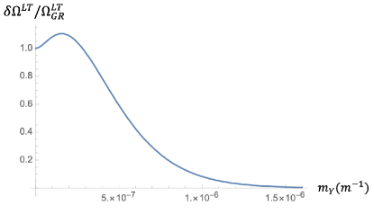
Figure 1: $\delta\Omega^{LT}/\Omega^{LT}_{GR}$ as a function of $m_{Y}$. Note that GR is recovered in the limit $m_{Y}\rightarrow\infty$

It shows the high accuracy needed to put physical constraints on the effective mass $m_{Y}$. In particular, the more accurate the measure, the narrower the allowed range of $m_{Y}$ will be.

The value of $m_{Y}$ shown in Eq. (45) is comparable with the LARES one, but it can be considered model independent, since it is a ’local’ measurement, which can be repeated at a different location, and does not require a gravity map of the Earth.

3.2 The PPN formalism in Horava–Lifshitz Gravity

Let us discuss now the weak-field limit of Horava–Lifshitz gravity to find out an explicit form for the gyroscopic and Lense–Thirring precessions. As pointed out in Horava:2010zj ; daSilva:2010bm , in order to be in agreement with Solar System observations and preserve the power-counting renormalizability at ultraviolet scales, the matter Lagrangian must be chosen carefully. In Horava:2010zj ; daSilva:2010bm , the authors propose the following general matter Lagrangian

$$\mathcal{L}_{M}=\tilde{N}\sqrt{\tilde{g}}\mathcal{L}_{M}\left(\tilde{N},\tilde{N}_{i},\tilde{g}_{ij};\psi_{n}\right)$$ (46)

where

$$\tilde{N} =\left(1-a_{1}\sigma\right)N$$ (47)

$$\tilde{N}^{i} =N^{i}+Ng^{ij}\nabla_{j}\phi$$

$$\tilde{g}_{ij} =\left(1-a_{2}\sigma\right)^{2}g_{ij}$$

$$\sigma =\frac{\mathscr{A}-\mathscr{B}}{N}$$

$$\mathscr{B} =-\dot{\phi}+N^{i}\nabla_{i}\phi+\frac{1}{2}N\nabla^{i}\phi\nabla_{i},\phi$$

with $a_{1}$, $a_{2}$ arbitrary constants. As previously pointed out, $\mathscr{A}$ is a gauge field depending on spatial coordinates and time, $N$ and $N^{i}$ are respectively Lapse and Shift functions, $g^{ij}$ is the three-dimensional metric. In the PPN formalism, the matter Lagrangian of this theory has a key role. Assuming a vanishing contribution of the cosmological constant $\Lambda=0$, the gyroscopic and Lense–Thirring precessions in Horava–Lifshitz gravity turn out to be related with those of GR through the relations Radicella:2014jwa :

$$\left|\frac{\Omega_{TOT}^{G}-\Omega^{G}_{GR}}{\Omega_{GR}^{G}}\right|=\left|\frac{2}{3}\left(\frac{G_{HL}}{G_{N}}a_{1}-\frac{a_{2}}{a_{1}}-1\right)\right|$$ (48)

and

$$\left|\frac{\Omega_{TOT}^{LT}-\Omega^{LT}_{GR}}{\Omega_{GR}^{LT}}\right|=\left|\frac{G_{HL}}{G_{N}}-1\right|,$$ (49)

where the standard Newton constant $G_{N}$ must be distinguished from the effective gravitational constant of Horava–Lifshitz gravity $G_{HL}$. In this way the measure on the Lense–Thirring precession can be used to constrain the effective gravitational constant, which, in turn, can be replaced in Eq. (48) to find a graphical relation between $a_{1}$ and $a_{2}$.

In order to adapt the GINGER measures to the Horava–Lifshitz gravity, in the weak-field limit, we consider the frequency difference of light for two beams circulating in a laser cavity in opposite directions. This can be recast as a time difference between the right-handed beam propagation time and the left-handed one, namely

$$\delta\tau=P\lambda\Omega_{S},$$ (50)

with

$$\Omega_{S}=-\frac{2\sqrt{g_{00}}}{P\lambda}\oint\frac{g_{0i}}{g_{00}}ds^{i}.$$ (51)

In the above equations, $P$ is the perimeter of the ring, $\lambda$ the laser wavelength, and $\Omega_{S}$ the splitting in terms of frequency between the two beams. Replacing the form of $g_{00}$ and $g_{0i}$ for Horava–Lifshitz gravity in Eq. (51), $\Omega_{S}$ turns out to be Radicella:2014jwa

$$\Omega_{S} = \frac{4A}{P\lambda}\Omega_{E}\left[\cos(\theta+\alpha)\right.$$ (52)

$$- \left(1+\frac{G_{HL}}{G_{N}}a_{1}-\frac{a_{2}}{a_{1}}\right)\frac{G_{HL}M}{R}\sin\alpha\sin\theta$$

$$- \left.\frac{G_{HL}I_{E}}{R^{3}}(2\cos\theta\cos\alpha+\sin\theta\sin\alpha)\right],$$

with $A$ being the area encircled by the light beams, $\alpha$ the angle between the local radial direction and the normal to the plane of the array-laser ring, $\theta$ the colatitude of the laboratory, $\Omega_{E}$ the rotation rate of the Earth as measured in the local reference frame and $I_{E}$ the Earth momentum of inertia. The first term in the RHS is the Sagnac term, the second is the gyroscopic term, while last is the Lense–Thirring term. Notice that by setting $G_{HL}=G_{N}$, the splitting in terms of frequency reduces to that of GR, as expected. The presence of two rings yields a dynamic measure of the angle, so that the overall precision of GINGER is 1/100 in the Lense–Thirring term and 1/1000 in the geodetic term. From Eq. (49), we obtain that the effective gravitational constant of Horava–Lifshitz gravity is related to the Newtonian constant through the numerical relation

$$0.999\,G_{N}<G_{HL}<1.001\,G_{N}$$ (53)

Setting $\displaystyle\frac{G_{HL}}{G_{N}}=0.999$ and replacing into Eq. (52), it turns out that the coupling constants $a_{1}$ and $a_{2}$ satisfy the relation

$$a_{1}(0.999a_{1}-0.99985)<a_{2}<a_{1}(0.999a_{1}-1.00015)$$

$$\text{if}\,\,\,a_{1}<0,$$

$$a_{1}(0.999a_{1}-1.00015)<a_{2}<a_{1}(0.999a_{1}-0.99985)$$

$$\text{if}\,\,\,a_{1}>0.$$ (54)

The graphical representation is shown in Fig. 2.

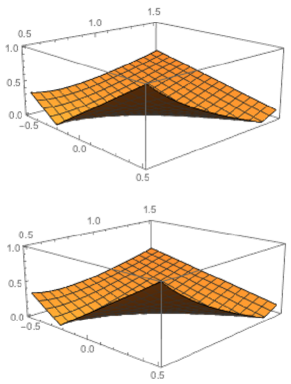
Figure 2: $\delta\Omega^{G}/\Omega^{G}_{GR}$ as a function of $a_{1}$ and $a_{2}$, with $G_{HL}/G_{N}$ fixed to $0.999$ (top) and 1.001 (bottom).

Similarly, by setting $\displaystyle\frac{G_{HL}}{G_{N}}=1.001$, we obtain

$$a_{1}(1.001a_{1}-0.99985)<a_{2}<a_{1}(1.001a_{1}-1.00015)$$

$$\text{if}\,\,\,a_{1}<0$$

$$a_{1}(1.001a_{1}-1.00015)<a_{2}<a_{1}(1.001a_{1}-0.99985)$$

$$\text{if}\,\,\,a_{1}>0.$$ (55)

The graphical representation is also reported in Fig 2. The ranges (54) and (55) can be obtained by considering the precision of GINGER in the geodesic term, that is expected to be 1 part in $10^{4}$. Moreover we only plotted ranges of $a_{1}$ and $a_{2}$ which can provide small corrections to GR. Indeed, we considered $a_{1}\in[0.5,1.5]$ and $a_{1}\in[-0.5,0.5]$, so that GR is recovered as soon as $a_{1}=1$ and $a_{2}=0$. In what follows, we let $G_{HL}/G_{N}$ varies between $0.999$ and $1.001$, which are the validity limits provided by the analysis of the Lense-Thirring term. Therefore, the relations between $a_{1}$, $a_{2}$ and $G_{HL}/G_{N}$, that is

$$\left|\frac{\Omega_{TOT}^{G}-\Omega^{G}_{GR}}{\Omega_{GR}^{G}}\right|=\left|\frac{2}{3}\left(\frac{G_{HL}}{G_{N}}a_{1}-\frac{a_{2}}{a_{1}}-1\right)\right|<10^{-4}$$ (56)

is plotted in Fig. 3,

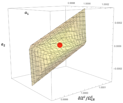
Figure 3: Graphical representation of Eq. (56). Red dot denotes the values of free parameters for which GR is recovered.

which shows numerical constraints to the matter Lagrangian of Horava–Lifshitz gravity. In order to uniquely find $a_{1}$ and $a_{2}$, a further analysis is needed. We aim to use GINGER data in future works, with the purpose to ameliorate the precision of the numerical values of the free parameters.

4 Discussion and Conclusions

We considered two modified theories of gravity and constrained the corresponding free parameters by GINGER experimental data. The former theory is based on extensions of the Hilbert–Einstein action, and belongs to the so-called Extended Theories of Gravity. Extending GR leads to higher–order field equations carrying for the gravitational field. From the weak-field limit of the theory, it is possible to relate the gyroscopic and Lense–Thirring precessions with the parameters of these further degrees of freedom. GINGER experimental data of these precessions put an upper limit to the first derivative of the function $f(R,R^{\mu\nu}R_{\mu\nu},\phi)$ with respect to the second-order curvature invariant $R^{\mu\nu}R_{\mu\nu}$. Specifically we get

$$m_{Y}\equiv\sqrt{\frac{1}{f_{Y}\left(0,0,\phi^{(0)}\right)}}\geq 1.88\cdot 10^{-6}m^{-1}.$$ (57)

If compared to the results provided by Lares and GP-B, we notice that GINGER can provide a stronger constraint to the effective mass with respect to the latter.

The second theory here discussed belongs to the class of alternative theories of gravity aimed to relax some assumptions of GR and to construct actions which better fit the high-energy shortcomings suffered by Einstein gravity. We considered a specific matter Lagrangian of Horava-Lifshitz gravity, which preserves the unitarity and allows to fit the Solar System observations. Such Lagrangian, in the most general form, introduces in the theory two arbitrary parameters $a_{1}$ and $a_{2}$, which cannot be theoretically constrained. We used the weak–field limit to find a relation between the two constants and the value of the effective gravitational constant in Horava–Lifshitz gravity. In particular, from the Lense-Thirring precession we obtain

$$0.999\,G_{N}<G_{HL}<1.001\,G_{N}.$$ (58)

By means of this result, it turns out that $a_{1}$ and $a_{2}$ can be fixed through data on Lense–Thirring precession, according to which relations (54) and (55) hold. Moreover, considering a precision of 1/10000 for the geodesic term, Eq. (56) provides a numerical relation between $a_{1}$, $a_{2}$ and $G_{HL}/G_{N}$, plotted in Fig. 3.

The analysis of this work represents a first step towards constraining modified theories of gravity and, in general, metric theories through GINGER data.

Some points need to be stressed in conclusion. With respect to results coming from satellites Capozziello:2014mea , GINGER measurements avoid issues related to the dynamical configurations of space-based experiments. For example, thanks to the experimental set up, errors and noise coming from considering fine gravity maps can be avoided. Finally, being the experiment essentially static, problems related to the timing and the synchronization between different reference frames (e.g. Earth and satellite) can be removed.

As final remark, we can say that relatively simple experiments like GINGER can achieve and ameliorate the performances of space-based setups in measuring gravitational parameters. This could be the starting point for a systematic investigation of theories of gravity by Earth-based experiments.

References

- (1) B. P. Abbott et al. [LIGO Scientific and Virgo], “Observation of Gravitational Waves from a Binary Black Hole Merger,” Phys. Rev. Lett. 116 (2016) no.6, 061102
- (2) B. P. Abbott et al. [LIGO Scientific and Virgo], “GW170817: Observation of Gravitational Waves from a Binary Neutron Star Inspiral,” Phys. Rev. Lett. 119 (2017) no.16, 161101
- (3) B. P. Abbott et al. [LIGO Scientific and VIRGO], “GW170104: Observation of a 50-Solar-Mass Binary Black Hole Coalescence at Redshift 0.2,” Phys. Rev. Lett. 118 (2017) no.22, 221101 [erratum: Phys. Rev. Lett. 121 (2018) no.12, 129901]
- (4) B. P. Abbott et al. [LIGO Scientific, Virgo, Fermi-GBM and INTEGRAL], “Gravitational Waves and Gamma-rays from a Binary Neutron Star Merger: GW170817 and GRB 170817A,” Astrophys. J. Lett. 848 (2017) no.2, L13
- (5) B. P. Abbott et al. [LIGO Scientific and Virgo], “GW170814: A Three-Detector Observation of Gravitational Waves from a Binary Black Hole Coalescence,” Phys. Rev. Lett. 119 (2017) no.14, 141101
- (6) K. Akiyama et al. [Event Horizon Telescope], “First M87 Event Horizon Telescope Results. I. The Shadow of the Supermassive Black Hole,” Astrophys. J. 875 (2019) no.1, L1
- (7) S. Weinberg, “Gravitation and Cosmology,” John Wiley Sons Inc. (1972), New York.
- (8) V. Sahni, “Dark matter and dark energy,” Lect. Notes Phys. 653 (2004), 141-180
- (9) R. Catena and P. Ullio, “A novel determination of the local dark matter density,” JCAP 08 (2010), 004
- (10) J. F. Navarro, C. S. Frenk and S. D. M. White, “The Structure of cold dark matter halos,” Astrophys. J. 462 (1996), 563-575
- (11) G. Bertone, D. Hooper and J. Silk, “Particle dark matter: Evidence, candidates and constraints,” Phys. Rept. 405 (2005), 279-390
- (12) T. Thiemann, “Modern canonical quantum general relativity,” [arXiv:gr-qc/0110034 [gr-qc]].
- (13) R. L. Arnowitt, S. Deser and C. W. Misner, “Canonical variables for general relativity,” Phys. Rev. 117 (1960), 1595-1602
- (14) C. W. Misner, “Quantum cosmology. 1.,” Phys. Rev. 186 (1969), 1319-1327
- (15) R. L. Arnowitt, S. Deser and C. W. Misner, “The Dynamics of general relativity,” Gen. Rel. Grav. 40 (2008), 1997-2027
- (16) F. Bajardi, D. Vernieri and S. Capozziello, “Bouncing Cosmology in f(Q) Symmetric Teleparallel Gravity,” Eur. Phys. J. Plus 135 (2020) no.11, 912
- (17) B. S. DeWitt, “Quantum Field Theory in Curved Space-Time,” Phys. Rept. 19 (1975), 295-357
- (18) T. Padmanabhan, “Gravity and the thermodynamics of horizons,” Phys. Rept. 406 (2005), 49.
- (19) E. Calzetta and B. L. Hu, “Closed Time Path Functional Formalism in Curved Space-Time: Application to Cosmological Back Reaction Problems,” Phys. Rev. D 35 (1987), 495
- (20) M.B. Green, J.H. Schwarz, E. Witten, “Superstring Theory”, Cambridge Univ. Press (1987), Cambridge.
- (21) P. Van Nieuwenhuizen, “Supergravity,” Phys. Rept. 68 (1981), 189-398
- (22) C. Kiefer, “Quantum gravity: A general introduction,” Lect. Notes Phys. 631 (2003), 3-13
- (23) S. W. Hawking, “Particle Creation by Black Holes,” Commun. Math. Phys. 43 (1975), 199-220 [erratum: Commun. Math. Phys. 46 (1976), 206]
- (24) J. D. Bekenstein, “Black holes and entropy,” Phys. Rev. D 7 (1973), 2333-2346
- (25) A. Strominger and C. Vafa, “Microscopic origin of the Bekenstein-Hawking entropy,” Phys. Lett. B 379 (1996), 99-104
- (26) G. W. Gibbons and S. W. Hawking, “Action Integrals and Partition Functions in Quantum Gravity,” Phys. Rev. D 15 (1977), 2752-2756
- (27) M. Banados, C. Teitelboim and J. Zanelli, “The Black hole in three-dimensional space-time,” Phys. Rev. Lett. 69 (1992), 1849-1851
- (28) A. H. Guth, “The Inflationary Universe: A Possible Solution to the Horizon and Flatness Problems,” Adv. Ser. Astrophys. Cosmol. 3 (1987), 139-148
- (29) A. D. Linde, “A New Inflationary Universe Scenario: A Possible Solution of the Horizon, Flatness, Homogeneity, Isotropy and Primordial Monopole Problems,” Adv. Ser. Astrophys. Cosmol. 3 (1987), 149-153
- (30) A. D. Linde, “Chaotic Inflation,” Phys. Lett. B 129 (1983), 177-181
- (31) A. H. Guth and S. Y. Pi, “Fluctuations in the New Inflationary Universe,” Phys. Rev. Lett. 49 (1982), 1110-1113
- (32) E. Elizalde, “Quantum vacuum fluctuations and the cosmological constant,” J. Phys. A 40 (2007), 6647-6655
- (33) N.D. Birrell and P.C.W. Davies, “Quantum Fields in Curved Space,” Cambridge Univ. Press. (1984), Cambridge
- (34) I. L. Buchbinder, S. D. Odintsov and I. L. Shapiro, “Effective action in quantum gravity,” Taylor Francis (1992) Boca Raton.
- (35) S. Capozziello and M. De Laurentis, “Extended Theories of Gravity,” Phys. Rept. 509 (2011), 167-321
- (36) D. Wands, “Extended gravity theories and the Einstein-Hilbert action,” Class. Quant. Grav. 11 (1994), 269-280
- (37) M. Crisostomi, K. Koyama and G. Tasinato, “Extended Scalar-Tensor Theories of Gravity,” JCAP 04 (2016), 044
- (38) T. Clifton, P. G. Ferreira, A. Padilla and C. Skordis, “Modified Gravity and Cosmology,” Phys. Rept. 513 (2012), 1-189
- (39) S. Nojiri and S. D. Odintsov, “Introduction to modified gravity and gravitational alternative for dark energy,” eConf C0602061 (2006), 06
- (40) F. Bajardi, S. Capozziello and D. Vernieri, “Non-local curvature and Gauss–Bonnet cosmologies by Noether symmetries,” Eur. Phys. J. Plus 135 (2020) no.12, 942
- (41) F. Bajardi and S. Capozziello, “ Noether cosmology,” Eur. Phys. J. C 80 (2020) no.8, 704
- (42) F. Bajardi, K. F. Dialektopoulos and S. Capozziello, “Higher Dimensional Static and Spherically Symmetric Solutions in Extended Gauss–Bonnet Gravity,” Symmetry 12 (2020) no.3, 372
- (43) F. Bajardi and S. Capozziello, “Noether Symmetries and Quantum Cosmology in Extended Teleparallel Gravity,” doi:10.1142/S0219887821400028
- (44) Y. F. Cai, S. Capozziello, M. De Laurentis and E. N. Saridakis, “f(T) teleparallel gravity and cosmology,” Rept. Prog. Phys. 79 (2016) no.10, 106901
- (45) R. T. Hammond, “Torsion gravity,” Rept. Prog. Phys. 65 (2002), 599-649
- (46) T. P. Sotiriou and S. Liberati, “Metric-affine f(R) theories of gravity,” Annals Phys. 322 (2007), 935-966
- (47) J. B. Jiménez, L. Heisenberg and T. S. Koivisto, “The Geometrical Trinity of Gravity,” Universe 5 (2019) no.7, 173
- (48) V. Vitagliano, T. P. Sotiriou and S. Liberati, “The dynamics of metric-affine gravity,” Annals Phys. 326 (2011), 1259-1273 [erratum: Annals Phys. 329 (2013), 186-187]
- (49) N. Frusciante, M. Raveri, D. Vernieri, B. Hu and A. Silvestri, “Hořava Gravity in the Effective Field Theory formalism: From cosmology to observational constraints,” Phys. Dark Univ. 13 (2016), 7-24
- (50) S. Capozziello, “Curvature quintessence,” Int. J. Mod. Phys. D 11 (2002), 483-492
- (51) T. P. Sotiriou and V. Faraoni, “f(R) Theories Of Gravity,” Rev. Mod. Phys. 82 (2010), 451-497
- (52) A. De Felice and S. Tsujikawa, “f(R) theories,” Living Rev. Rel. 13 (2010), 3
- (53) A. A. Starobinsky, “Disappearing cosmological constant in f(R) gravity,” JETP Lett. 86 (2007), 157-163
- (54) S. Nojiri and S. D. Odintsov, “Modified f(R) gravity consistent with realistic cosmology: From matter dominated epoch to dark energy universe,” Phys. Rev. D 74 (2006), 086005
- (55) S. Capozziello, S. Nojiri, S. D. Odintsov and A. Troisi, “Cosmological viability of f(R)-gravity as an ideal fluid and its compatibility with a matter dominated phase,” Phys. Lett. B 639 (2006), 135-143
- (56) G. Cognola, E. Elizalde, S. Nojiri, S. D. Odintsov, L. Sebastiani and S. Zerbini, “A Class of viable modified f(R) gravities describing inflation and the onset of accelerated expansion,” Phys. Rev. D 77 (2008), 046009
- (57) S. Capozziello, C. A. Mantica and L. G. Molinari, “Cosmological perfect-fluids in f(R) gravity,” Int. J. Geom. Meth. Mod. Phys. 16 (2018) no.01, 1950008
- (58) S. Capozziello, G. Gionti, S.J. and D. Vernieri, “String duality transformations in gravity from Noether symmetry approach,” JCAP 01 (2016), 015
- (59) A. Borowiec, S. Capozziello, M. De Laurentis, F. S. N. Lobo, A. Paliathanasis, M. Paolella and A. Wojnar, “Invariant solutions and Noether symmetries in Hybrid Gravity,” Phys. Rev. D 91 (2015) no.2, 023517
- (60) A. Stabile, A. Stabile and S. Capozziello, “Conformal Transformations and Weak Field Limit of Scalar-Tensor Gravity,” Phys. Rev. D 88 (2013) no.12, 124011
- (61) R. Aldrovandi and J. G. Pereira, “Teleparallel Gravity: An Introduction,” Fundam. Theor. Phys. 173 (2013)
- (62) A. Conroy and T. Koivisto, “The spectrum of symmetric teleparallel gravity,” Eur. Phys. J. C 78 (2018) no.11, 923
- (63) P. Horava, “Quantum Gravity at a Lifshitz Point,” Phys. Rev. D 79 (2009), 084008
- (64) S. Moseley, N. Scaramuzza, J. D. Tasson, and M. L. Trostel, Phys. Rev. D 100, 064031 (2019).
- (65) S. Capozziello and F. Bajardi, “Gravitational waves in modified gravity,” Int. J. Mod. Phys. D 28 (2019) no.05, 1942002
- (66) S. Capozziello, V. F. Cardone and A. Troisi, “Low surface brightness galaxies rotation curves in the low energy limit of r**n gravity: no need for dark matter?,” Mon. Not. Roy. Astron. Soc. 375 (2007), 1423-1440
- (67) S. Capozziello, V. F. Cardone, S. Carloni and A. Troisi, “Can higher order curvature theories explain rotation curves of galaxies?,” Phys. Lett. A 326 (2004), 292-296
- (68) J. Santos, J. S. Alcaniz, M. J. Reboucas and F. C. Carvalho, “Energy conditions in f(R)-gravity,” Phys. Rev. D 76 (2007), 083513
- (69) T. P. Sotiriou, “Covariant Effective Action for Loop Quantum Cosmology from Order Reduction,” Phys. Rev. D 79 (2009), 044035
- (70) A. V. Astashenok, S. Capozziello, S. D. Odintsov and V. K. Oikonomou, “Extended Gravity Description for the GW190814 Supermassive Neutron Star,” Phys. Lett. B 811 (2020) 135910
- (71) L. Lombriser and A. Taylor, “Breaking a Dark Degeneracy with Gravitational Waves,” JCAP 03 (2016), 031
- (72) S. Capozziello, G. Lambiase, M. Sakellariadou and A. Stabile, “Constraining models of extended gravity using Gravity Probe B and LARES experiments,” Phys. Rev. D 91 (2015) no.4, 044012
- (73) A. Tartaglia, A. Di Virgilio, J. Belfi, N. Beverini and M. L. Ruggiero, “Testing general relativity by means of ring lasers,” Eur. Phys. J. Plus 132 (2017) no.2, 73
- (74) A. D. V. Di Virgilio, F. Bosi, U. Giacomelli, A. Simonelli, G. Terreni, A. Basti, N. Beverini, G. Carelli, D. Ciampini and F. Fuso, et al. “Underground Sagnac gyroscope with sub-prad/s rotation rate sensitivity: Toward general relativity tests on Earth,” Phys. Rev. Res. 2 (2020) no.3, 032069
- (75) A. D. V. Di Virgilio, J. Belfi, W. T. Ni, N. Beverini, G. Carelli, E. Maccioni and A. Porzio, “GINGER: A feasibility study,” Eur. Phys. J. Plus 132 (2017) no.4, 157
- (76) M. L. Ruggiero, “Sagnac Effect, Ring Lasers and Terrestrial Tests of Gravity,” Galaxies 3 (2015) no.2, 84-102
- (77) F. Bosi, A. D. V. Di Virgilio, U. Giacomelli, A. Simonelli, G. Terreni, A. Basti, N. Beverini, G. Carelli, D. Ciampini and F. Fuso, et al. “Sagnac gyroscopes, GINGERINO, and GINGER,” J. Phys. Conf. Ser. 1468 (2020) no.1, 012243
- (78) A. D. V. Di Virgilio, U. Giacomelli, A. Simonelli, G. Terreni, A. Basti, N. Beverini, G. Carelli, D. Ciampini, F. Fuso and E. Maccioni, et al. “Reaching the sensitivity limit of a Sagnac gyroscope through linear regression analysis,” [arXiv:2101.08179 [gr-qc]].
- (79) A. Stepanian, S. Khlghatyan and V. G. Gurzadyan, Eur. Phys. J. C 80 (2020) no.11, 1011 doi:10.1140/epjc/s10052-020-08560-0 [arXiv:2010.07472 [gr-qc]].
- (80) V. G. Gurzadyan and A. T. Margaryan, arXiv:2009.07689 [astro-ph.IM].
- (81) A. A. Starobinsky, “A New Type of Isotropic Cosmological Models Without Singularity,” Adv. Ser. Astrophys. Cosmol. 3 (1987), 130-133
- (82) A. A. Starobinsky, “Dynamics of Phase Transition in the New Inflationary Universe Scenario and Generation of Perturbations,” Phys. Lett. B 117 (1982), 175-178
- (83) P. A. R. Ade et al. [Planck], “Planck 2015 results. XIV. Dark energy and modified gravity,” Astron. Astrophys. 594 (2016), A14
- (84) F. Bajardi and S. Capozziello, “Equivalence of nonminimally coupled cosmologies by Noether symmetries,” Int. J. Mod. Phys. D 29 (2020) no.14, 2030015
- (85) P. Horava, “Spectral Dimension of the Universe in Quantum Gravity at a Lifshitz Point,” Phys. Rev. Lett. 102 (2009), 161301
- (86) H. Lu, J. Mei and C. N. Pope, “Solutions to Horava Gravity,” Phys. Rev. Lett. 103 (2009), 091301
- (87) G. Calcagni, “Cosmology of the Lifshitz universe,” JHEP 09 (2009), 112
- (88) C. Charmousis, G. Niz, A. Padilla and P. M. Saffin, “Strong coupling in Horava gravity,” JHEP 08 (2009), 070
- (89) R. Brandenberger, “Matter Bounce in Horava-Lifshitz Cosmology,” Phys. Rev. D 80 (2009), 043516
- (90) T. P. Sotiriou, M. Visser and S. Weinfurtner, “Quantum gravity without Lorentz invariance,” JHEP 10 (2009), 033
- (91) R. G. Cai, L. M. Cao and N. Ohta, “Topological Black Holes in Horava-Lifshitz Gravity,” Phys. Rev. D 80 (2009), 024003
- (92) G. Panotopoulos, D. Vernieri and I. Lopes, “Quark stars with isotropic matter in Hořava gravity and Einstein–æther theory,” Eur. Phys. J. C 80 (2020) no.6, 537
- (93) D. Vernieri, “Anisotropic fluid spheres in Hořava gravity and Einstein-æther theory with a nonstatic æther,” Phys. Rev. D 100 (2019) no.10, 104021
- (94) T. P. Sotiriou, I. Vega and D. Vernieri, “Rotating black holes in three-dimensional Hořava gravity,” Phys. Rev. D 90 (2014) no.4, 044046
- (95) A. Kehagias and K. Sfetsos, “The Black hole and FRW geometries of non-relativistic gravity,” Phys. Lett. B 678 (2009), 123-126
- (96) T. Harko, Z. Kovacs and F. S. N. Lobo, “Solar system tests of Horava-Lifshitz gravity,” Proc. Roy. Soc. Lond. A 467 (2011), 1390-1407
- (97) C. W. F. Everitt, D. B. DeBra, B. W. Parkinson, J. P. Turneaure, J. W. Conklin, M. I. Heifetz, G. M. Keiser, A. S. Silbergleit, T. Holmes and J. Kolodziejczak, et al. “Gravity Probe B: Final Results of a Space Experiment to Test General Relativity,” Phys. Rev. Lett. 106 (2011), 221101
- (98) P. Horava and C. M. Melby-Thompson, “General Covariance in Quantum Gravity at a Lifshitz Point,” Phys. Rev. D 82 (2010), 064027
- (99) A. M. da Silva, “An Alternative Approach for General Covariant Horava-Lifshitz Gravity and Matter Coupling,” Class. Quant. Grav. 28 (2011), 055011
- (100) N. Radicella, G. Lambiase, L. Parisi and G. Vilasi, “Constraints on Covariant Horava-Lifshitz Gravity from frame-dragging experiment,” JCAP 12 (2014), 014
- (101) I. Quandt and H. J. Schmidt, “The Newtonian limit of fourth and higher order gravity,” Astron. Nachr. 312 (1991), 97
- (102) S. Nojiri and S. D. Odintsov, “Modified Gauss-Bonnet theory as gravitational alternative for dark energy,” Phys. Lett. B 631 (2005), 1-6
- (103) M. De Laurentis and A. J. Lopez-Revelles, “Newtonian, Post Newtonian and Parameterized Post Newtonian limits of f(R, G) gravity,” Int. J. Geom. Meth. Mod. Phys. 11 (2014), 1450082
- (104) A. Stabile, “The most general fourth order theory of Gravity at low energy,” Phys. Rev. D 82 (2010), 124026