Water entry and exit of 2D and axisymmetric bodies

Abstract

The present paper is dedicated to the development of a numerical model for the water impact of two-dimensional (2D) and axisymmetric bodies with imposed motion. The work is a first step towards the implementation of a 2D+t procedure to be used for the analysis of aircraft ditching. The problem is investigated under the assumptions of an inviscid and incompressible fluid, which is modelled by a potential flow model with fully non-linear boundary conditions at the free-surface. The unsteady boundary value problem with a free-surface is numerically solved through a boundary element method, coupled to a simplified finite element method to describe the thinnest part of the jet. The study is aimed at describing the entry and exit phases. Specific numerical solutions are developed to tackle the exit phase and to improve the stability of the model. Results are presented in terms of free-surface shape, pressure distribution and hydrodynamic load acting on the impacting body. The model is used to study the water entry and exit of a 2D wedge and an axisymmetric cone, for which numerical or experimental results are available in the literature. The numerical investigation shows that the proposed model accurately simulate both the entry and exit phases. For the exit phase, it is shown that the proposed model, being fully non-linear, provides a much better prediction of the loads and the wetted area compared to simplified (analytical) approaches. The effects of the gravity, usually missing in the approaches available in the literature, are also investigated, showing they are rather important, especially, in the exit phase.

© 2021. This manuscript version is made available under the CC-BY-NC-ND 4.0 license

http://creativecommons.org/licenses/by-nc-nd/4.0/

1 Introduction

Aircraft ditching, despite being a rare event, has to be accounted for in the design and certification phases of new aircrafts to guarantee the safety of the occupants. Large-scale experimental tests are very expensive and impractical. Therefore, aircraft manufacturers need computational tools able to provide a satisfactorily accurate description of the hydrodynamics and of the resulting fluid-structure interaction during the ditching phase, which govern both the aircraft dynamics and the structural response. During the design and certification phases, especially when many different configurations have to be analyzed, besides the high fidelity, fully coupled, fluid and structural solvers, fast and efficient solvers, although approximate, are strongly necessary to reduce the computational effort. A possibile solution is to describe the ditching phenomena with a 2D+t procedure, largely used in the past in the naval application, e.g. [1], and recently applied to aircraft ditching application as well [2, 3]. In such a procedure the 3D problem is approximated by a 2D problem in the transverse plane in an earth-fixed frame of reference, with the shape of the impacting body changing in time. That is, the problem is described by a series of 2D water-impact problems, by neglecting the longitudinal derivatives of the hydrodynamic unknowns. Despite the approximations, this approach provides reasonably accurate information on the loads acting on the body. By looking at the ditching problem from a 2D+t perspective, in the rear part of the advancing fuselage the cross section shrinks and the lowest point of the contour rises, thus resembling a water exit problem. As such, the 2D solver used in the procedure must be able to handle both the entry and exit phases. These phases are characterized by a rapid evolution of the wetted surface which expands during the entry phase, when the body contour moves downwards, whereas it shrinks during the exit phase, when the body contour moves upwards. Moreover, in the combined water entry and exit problem, suction loads (hydrodynamic pressures being below the atmospheric pressure) can be observed. The suction loads increase as the body decelerates during the entry phase and, if the body deceleration is constant, they reach their maximum value at the transition between the entry and exit phase [4]. However, CFD results presented in [5] for a rigid wedge show that the peak can occur before the beginning of the exit phase if the jet root starts separating from the body during the entry phase. So, the suction load and the flow separation can be closely related, and they can also appear in other problems, such as the oblique water entry of wedges [6] and curved bodies at high horizontal speed [7]. Recent experimental tests on the combined water entry and exit problem of axisymmetric bodies also show the influence of the gravity on the exit phase [8]. The previuos paper also presents experimental tests on pure water exit of a body initially submerged. Pure water exit problems were investigated with experiments in [9] and through a potential flow model in [10, 11].
The first analytical model for the description of the combined water entry and exit events was proposed in [12]. In this paper, the original Wagner model [13] was used for the entry stage whereas during the exit phase the same model was modified by discarding the ”slamming term” (depending on the body velocity) and considering only the ”added mass term” (depending on the body acceleration). In [14] the problem is solved via a linearized form of the mixed boundary value problem and by enforcing a Kutta-type condition at the contact point during the exit stage. The contact point position is predicted by assuming the proportionality between the speed of contraction of the wetted surface and the velocity of the particles located at the contact points. The latter model was extended in [15] to include body motions with time-dependent acceleration and water exit of a body whose shape changes in time. A semi-analytical model was proposed in [4] as a combination of the Modified Logvinovich Model (MLM), for the entry phase, and a modified von Kármán model, for the exit phase. In the second one, the position of the contact point is given by the intersection between the body and a reference water level corresponding to the maximum vertical position of the contact point reached during the entry phase. The pressure is evaluated with the MLM, but only the terms depending on the body acceleration are retained during the exit stage. Methods [15] and [4] were compared in [8] with experimental results of the water entry/exit of a rigid cone, highlighting the limits of analytical models partly due to the lack of gravity effects.
In this paper the idea is to use the fully non-linear, two-dimensional incompressible potential flow model proposed in [16] and [17], and already used for the water entry problem with constant velocity. The use of fully non-linear boundary conditions at the free-surface enables an accurate prediction of the pressure distribution at the spray root, which can be important when modelling the fluid-structure interaction. In [16] the problem is formulated via a boundary-element representation of the velocity potential (BEM model) and the time evolution is described by a mixed Eulerian-Lagrangian approach, originally proposed in [18]. The free-surface evolution is followed using a Lagrangian approach by integrating in time the kinematic boundary condition. The model has been validated in the case of 2D and axisymmetric body impact with constant velocity [16]. In the latter paper, the thin jet, generated by the flow singularity about the intersection between the free-surface and the body contour, is cut off and replaced by a straight panel orthogonal to the solid boundary with a suitable boundary condition applied there, as proposed in [19]. This assumption is justified as the pressure inside the thin jet is rather negligible, despite the high computational effort needed for an accurate description of the flow in such a thin region. In [20] the model proposed in [19] was extended to describe the flow in presence of flow separation by enforcing a Kutta condition as soon as the jet truncation passes through the separation point: it is assumed that the fluid leaves the separation point tangentially and with a finite velocity. The proposed model was successfully applied to the case of body contours with geometry singularities, such as knuckles. To achieve an improved prediction of the flow separation but limiting the high computational effort, [17] presents a simplified hybrid BEM-FEM model (as an evolution of the BEM solver in [16]), which models the thinnest part of the jet with control volumes where the velocity potential is represented as a harmonic polynomial representation. The model is validated in [17] for the water entry with constant velocity of a wedge with different deadrise angles and in [21], also for separated flows, solved by using the Kutta condition at the separation point.
Here, the hybrid BEM-FEM model is extended to deal with the combined water entry and exit problem. The numerical simulation of the exit phase is critical, especially if subsequent to a water entry phase, and free-surface instabilities might arise, as observed in CFD simulations in [5] and potential flow simulations in [22]. These instabilities are quite difficult to manage and can cause the stop of the numerical simulation. For this reason, two techniques used in the original model for the water entry at constant velocity [16] are further extended and exploited here to improve the stability of the numerical solution during the exit phase. The first one cuts the jet when its thickness becomes too thin, whereas the second one increases the action of the numerical filter used to overcome the saw-tooth instability of the BEM solution [23]. Furthermore, in the original hybrid BEM-FEM approach, the gravity effects were not included, because it was used only in the water entry problems at constant velocity, where the gravity effects are negligible. Here, in order to enable the model to deal also with the exit phase, the gravity effects are included.
The proposed model is validated against two different test cases, a rigid 2D wedge and a rigid cone, with imposed motion combining water entry and exit phases. For the wedge case, the present results are compared with CFD [24] and semi-analytical [4] computations, in terms of non-dimensional vertical force, whereas, for the cone case, the vertical force and the contact line time histories are compared with experimental and analytical results presented in [8]. Results, in terms of free-surface evolution and pressure distribution, are also presented.

2 Hybrid BEM-FEM formulation

The vertical water impact problem of 2D and axisymmetric bodies is here investigated. The study is conducted in an earth-fixed frame of refercence, with $y$ the horizontal axis oriented from left to right, $y=0$ being at the symmetry axis, and $z$ the vertical axis oriented upwards, with $z=0$ located at the still water level. Owing to the symmetry of the problem, only the right half of the plane ($y,z$) is considered (see Fig. 1).

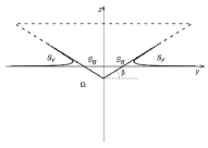
Figure 1: Sketch of the problem

The fluid domain $\Omega$ is therefore bounded by the free surface, $S_{F}$, on the top and by the body surface, $S_{B}$, on the left, and it is assumed infinitely deep. The impacting body is characterized by the deadrise angle $\beta$, which is the angle between the body surface and the horizontal axis. Under the hypotheses of an incompressible fluid and irrotational flow, the hydrodynamic problem can be formulated in terms of the velocity potential, $\varphi$, which satisfies the Laplace equation in the fluid domain $\Omega$, the Neumann boundary condition on the body surface, and a Dirichelet boundary condition on the free surface $S_{F}$. The former comes from the impermeability of the body contour; the latter is written in terms of a dynamic boundary condition, which simply states that the pressure is constant over the free-surface. The free-surface position is determined as a part of the problem by integrating in time the kinematic boundary condition, (particles located at the free-surface remain at the free-surface). The boundary value problem reads as follows

$${\nabla^{2}\varphi}=0\hskip 99.58464pt\Omega$$ (1)

$${\frac{\partial\varphi}{\partial n}}={\mathbf{V}\cdot\mathbf{n}}\hskip 85.35826ptS_{B}$$

$${\frac{D\varphi}{Dt}}={\frac{\left|\nabla\varphi\right|^{2}}{2}-gz}\hskip 56.9055ptS_{F}$$

$${\frac{D\mathbf{x}}{Dt}}=\mathbf{u}\hskip 99.58464ptS_{F}$$

where $\mathbf{V}$ is the body vertical velocity (positive downwards), $\mathbf{n}$ is the unit vector normal to the boundary of the fluid domain oriented inwards, $\frac{D}{Dt}$ is the total derivative with respect to time $t$, $\mathbf{x}$ denotes the position of a particle lying at the free-surface, and $\mathbf{u}$ the velocity at $\mathbf{x}$. Although the effect of the acceleration of gravity, $g$, are usually neglected in water entry problems, especially for the constant water entry problem where $gt/U<<1$, they are accounted for in the present study to assess the role of the gravity in water entry/exit problems. The surface-tension effects are always neglected. According to the boundary value problem (1), the velocity potential is known on the free-surface, whereas its normal derivative is assigned on the body contour. The problem is solved through a mixed Eulerian-Lagrangian approach [18]. In order to solve the boundary value problem (1), the velocity potential is written in terms of a Boundary Integral Representation. The velocity potential on the body contour and its normal derivative on the free-surface are retrieved by writing the boundary integral representation at the boundary of the fluid domain. In this way, the problem takes the form of a boundary integral equation of mixed first and second kind [16]

$$\frac{1}{2}\varphi(P)=\int_{S_{B}\bigcup S_{F}}{\left(\frac{\partial\varphi(Q)}{\partial n}G(P,Q)-\varphi(Q)\frac{\partial G(P,Q)}{\partial n}\right)dS(Q)}\hskip 28.45274ptP\in\Omega$$ (2)

where $G$ is the free-space Green’s function of the Laplace operator which in two dimensions is

$$G(P,Q)=\frac{1}{2\pi}log\left(\left|P-Q\right|\right),$$ (3)

whereas in three dimensions is

$$G(P,Q)=-\frac{1}{4\pi\left|P-Q\right|}.$$ (4)

The hydrodynamic load acting on the body is obtained by integration of the pressure distribution along the wetted part of the body. The pressure is computed by the unsteady Bernoulli’s equation:

$$p-p_{inf}=-\rho\left(\frac{\partial\varphi}{\partial t}+\frac{\left|\nabla\varphi\right|^{2}}{2}+gz\right)$$ (5)

where $\rho$ is the fluid density, equal to 1000 Kg/m³, and $p_{inf}$ is assumed null. The velocity potential along the body is deteminated using equation (2), whereas the time derivative of the velocity potential along the body, $\frac{\partial\varphi}{\partial t}$, is computed by formulating a boundary value problem similar to (1). The time derivative of the velocity potential is also a harmonic function which satisfies the following Dirichlet condition at the free-surface:

$$\frac{\partial\varphi}{\partial t}=-\frac{\left|\nabla\varphi\right|^{2}}{2}-gz$$ (6)

which comes from the constant pressure condition. A Neumann boundary condition applies on the body side, which is derived from the time derivative of the second equation in (1)

$$\frac{\partial}{\partial n}\left(\frac{\partial\varphi}{\partial t}\right)=\mathbf{n}\cdot\mathbf{a}-\mathbf{n}\cdot\left(\mathbf{V}\cdot\nabla\right)\mathbf{u}$$ (7)

The latter equation is rigorously valid only when the normal unit vector, $\mathbf{n}$, does not vary in time due to body rotations or deformations. In equation (7), $\mathbf{a}$ is the body acceleration and $\mathbf{u}$ is the fluid velocity along the body contour. As shown in [16], the term $\mathbf{n}\cdot\left(\mathbf{V}\cdot\nabla\right)\mathbf{u}$ can be written as

$$\mathbf{n}\cdot\left(\mathbf{V}\cdot\nabla\right)\mathbf{u}=V_{s}\frac{\partial u_{n}}{\partial s}-V_{n}\frac{\partial u_{s}}{\partial s}+k_{sn}\mathbf{V}\cdot\mathbf{u}$$ (8)

in the two-dimensional case and as

$$\mathbf{n}\cdot\left(\mathbf{V}\cdot\nabla\right)\mathbf{u}=V_{s}\frac{\partial u_{n}}{\partial s}-V_{n}\frac{\partial u_{s}}{\partial s}+k_{sn}V_{s}u_{s}+(k_{sn}+k_{\theta n})V_{n}u_{n}-\frac{r^{\prime}}{r}V_{n}u_{s}$$ (9)

in the three-dimensional case, where $\frac{\partial}{\partial s}$ denotes the spatial differentiation with respect to the tangent to the body contour, $k_{sn}$ and $k_{\theta n}$ denote the local curvatures of the body contour, $r$ is the radial position and in $r^{\prime}$, prime denotes differentiation along the meridian contour. The terms $\left\{u_{s},u_{n}\right\}$ and $\left\{V_{s},V_{n}\right\}$ are the projections of the fluid and body velocities along the tangent and the normal to the body contour, respectively.
The boundary integral equation (2) is solved via a zero-order panel method with a piecewise constant distribution of the variables on each panel. In the numerical model, the impacting body is represented as a set of discrete points which are interpolated with a cubic spline. At each time, step a linear extrapolation of the positions of the free-surface centroids is used to intersect the body contour and to locate the contact point and to identify the wetted area $S_{B}$ and the free-surface $S_{F}$. The first one is discretizated with straight line panels placing the vertices on the body spline curve. The same is done for the free-surface, where the panel vertices are located along the cubic spline built by interpolating the free-surface centroids position. The discretization of the fluid boundary is started from the intersection point of the free-surface with the body contour and the panel size increases linearly moving away from it. In the discrete form the influence coefficients of a panel on a panel midpoint are evaluated analytically in the 2D case, while in the axisymmetric case the integration is performed analytically in the azimuthal direction and numerically (through a Gauss formula with an even number of points) along the meridian section of the panel [16]. The use of an even number of points into the Gauss formula allows to avoid the singularity of the kernel, and to mimic the computation of the integral as a Cauchy Principal value. The solution of the boundary value problem provides the velocity potential on the wetted body contour and its normal derivative on the free-surface. The latter, along with the tangential velocity obtained by a second-order finite differences of the velocity potential along the boundary, defines the velocity at the free-surface. This velocity is used into the kinematic and dynamic boundary conditions to compute the free-surface shape and the velocity potential on it. The integration in time of the kinematic and dynamic conditions is done with a second-order Runge-Kutta scheme. The time step is chosen so as to satisfy two different conditions. The first one is to ensure that the maximum displacement of the centroid is smaller that a fraction of the panel length. The second one, which is active mainly in the early stage, is to prevent the panel centroids from penetrating the body. The new configuration of the fluid boundary is found by moving the body contour and the free-surface centroids in a Lagrangian way and by discretizing the new $S_{B}$ and $S_{F}$ as mentioned above. It is worth remarking that, although the boundary-value problem (1) is numerically satisfied at the midpoint of the panels, which are delimited by the vertices lying on the spline curve, Lagrangian markers, which are the centroids, used to track the free-surface motion are always located along the spline curve, thus enabling improved mass conservation properties of the numerical scheme [19].
In order to model the occurrence of flow separation, a Kutta condition is enforced at the separation point requiring that the flow leaves the body contour tangentially [21, 20]. In particular, a Neumann condition is applied at the first panel of the separated region, requiring that the normal velocity equals that of the last panel still attached to the body [21]. For body shapes with hard chines, such as a finite wedge or a cone, in the case of constant entry velocity the separation point can be assigned a priori and corresponds to the point of geometric singularity. If the body decelerates, such as in the cases studied in the following, the separation may be anticipated and the separation point is unknown and has to be determined as a part of the solution. The same happens for the water entry of convex-shaped bodies, such as a circular cylinder, when, even in the constant entry velocity case, the flow separates. For the latter case, a separation approach based on the negative pressure was proposed in [25] where the flow is assumed to detach from the body surface when the pressure becomes lower than the atmospheric value in a large part of the wetted area. However, negative pressure may occur without flow separation as shown in [15] for a rigid plate. Therein, it is also shown that, in the later stage of the deceleration, the pressure is negative over a large portion of the wetted area. Experimental evidence of negative pressures occurring without flow separation is provided in [26]. For these reasons, it is preferred here to assume that the separation point occurs only at the chine of the body.

2.1 Jet Model

As aforesaid, the flow singularity at the intersection between the free-surface and the body [27] leads to the formation of a thin jet layer along the body surface. If solved via BEM, the discretization of such a thin jet would require a panel size comparable to the jet thickness, and because of the local high speed of the fluid, a quite small time step would be necessary to preserve the stability and accuracy of the integration scheme. As a consequence, the computational effort would increase substantially. Moreover, due to the quite small angle at the jet tip, there is always a region where the boundary element method fails, regardless of the size of the panels. In order to overcome such important limitations, a common strategy is to cut the jet and replace it with a panel orthogonal to the body contour where appropriate boundary conditions are applied [16]. Since the pressure inside the thin jet is almost uniform, the jet cutting strategy still provides accurate estimates of the hydrodynamic loading. However, the cutting procedure may have limitations, as mentioned in [17] and then, if used, the fluid motion details inside the thin jet would be lost, leading for instance to an inaccurate prediction of the separation phase. For these reasons, the thin jet is here modelled using the simplified model proposed in [17, 21] and validated in the case of water entry with constant velocity of a finite wedge.
A portion of the jet region, starting from the tip, is discretized with small control volumes (Fig.2). The vertices of each volume $i$ correspond to the panel centroids on the body ($\hat{P}_{i-1},\hat{P}_{i}$) and on the free-surface ($\bar{P}_{i-1},\bar{P}_{i}$).

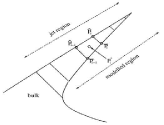
Figure 2: Sketch of the Jet Model

Inside each control volume the velocity potential is written in the form of a harmonic polynomial series, up to second order, about the corresponding centroid ($y^{*},z^{*}$)

$$\varphi_{i}^{j}(y,z)=A_{i}+B_{i}(y-y^{*})+C_{i}(z-z^{*})+\frac{1}{2}D_{i}\left[(y-y^{*})^{2}-(z-z^{*})^{2}\right]+E_{i}(y-y^{*})(z-z^{*})$$ (10)

Equation (10) introduces five additional unknowns, $A_{i},..,E_{i}$, for each control volume which require five additional equations. Four of them are derived by enforcing the boundary conditions at the body and free surface sides

$$\varphi_{i,n}^{j}(\hat{P}_{i-1})=\varphi_{,n}(\hat{P}_{i-1}),\hskip 8.5359pt\varphi_{i,n}^{j}(\hat{P}_{i})=\varphi_{,n}(\hat{P}_{i}),\hskip 8.5359pt\varphi_{i}^{j}(\bar{P}_{i-1})=\varphi(\bar{P}_{i-1}),\hskip 8.5359pt\varphi_{i}^{j}(\bar{P}_{i})=\varphi(\bar{P}_{i})$$ (11)

where $\varphi_{i,n}^{j}$ is the normal derivative of the velocity potential provided by the harmonic expression. The fifth equation is derived by enforcing the continuity of the normal derivative of the velocity potential at adjacent elements

$$\varphi_{i,n}^{j}(\hat{P}_{i-1})=\varphi_{(i-1),n}^{j}(\hat{P}_{i-1})$$ (12)

The set of equations (11) and (12) are coupled with the discretized form of the boundary integral equation (2) used in the remaining part of the fluid domain (hereinafter referred to as the “bulk” of the fluid). The jet model is activated only when the thin jet has already developed. Starting from the matching point with the modelled region, the bulk region is discretizated as mentioned earlier. A similar approach is adopted to discretize the modelled portion of the jet. The panel size is increased linearly, with a growth factor generally higher than that used for the free surface in the bulk of the domain. The hybrid BEM-FEM approach is also used for the evaluation of the time derivative of the velocity potential. Further details of the jet model are provided in [17, 21].

2.2 Water exit phase

A major difficulty in the simulation of the exit phase comes from the development of numerical instabilities in the free-surface profile shortly after the start of the exit phase. Such instabilities develop in time and eventually lead to a crash of the simulation. In order to preserve the stability of the numerical solution, two different strategies, which involve the use of techniques already used in the case of water entry at constant velocity [16], have been developed, which can either operate independently or in combination. Both of strategies are not activated at the beginning of the exit phase, when the body velocity is zero, but when the exit phase has already started, thus allowing a smoother transition between the entry and exit phases. In the present case, the strategies are activated when $V/V_{0}\leq-0.10$.
The first strategy consists in cutting the thin jet during the exit phase. This is justified as the jet length keeps increasing whereas the jet root shrinks. As a consequence, the jet becomes thinner and thinner and its description becomes more and more difficult. On the other hand, as in the entry phase, the pressure in the jet region is essentially zero, and thus cutting the jet has no effects on the hydrodynamic loading. Furthermore, while in the entry phase the description of the jet is needed to achieve a more accurate description of the flow separation, particularly from smoothly curved contours, in the exit phase the separation, if any, has already occurred and thus there is no need for an accurate description of the thin jet.

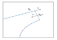
Figure 3: Cut procedure

When the jet is cut off, a new panel ($N_{B}+1$), orthogonal to the local body surface, is introduced (Fig.3): as the thinnest part of the jet is cut off, there is no need to use the hybrid BEM-FEM approach and the pure BEM is used everywhere in the fluid domain. There are two unknowns on the truncation panel: the velocity potential is derived from the solution of the boundary value problem whereas an additional equation is introduced for the normal derivative of the velocity potential at the panel $N_{B}+1$, which is imposed to be equal to the tangential derivative of the velocity potential along the body contour at the panel $N_{B}$,

$$\frac{\partial\varphi}{\partial n}(N_{B+1})=-\frac{\partial\varphi}{\partial s}(N_{B})$$ (13)

The negative sign accounts for the different orientations of the unit vectors $\mathbf{s}$ and $\mathbf{n}$.
The second strategy is to increase, during the exit phase, the action of the numerical filter used to overcome the saw-tooth instabilities. The smoothing formula used in the model was proposed in [23] and it is applied to the function $f(\xi)$ by subtracting the value of $\delta_{M}(\xi)$:

$$f(\xi)=f(\xi)-\delta_{M}(\xi)$$ (14)

The value of $\delta_{M}(\xi)$ depends on the order $m$ of the filter, which involves the $M=2m+1$ consecutive panels $(\xi-m,..,\xi,..,\xi+m)$, as follows:

$$\begin{pmatrix}2^{2}\delta_{3}\\ 2^{4}\delta_{5}\\ 2^{6}\delta_{7}\\ 2^{8}\delta_{9}\\ 2^{10}\delta_{11}\\ 2^{12}\delta_{13}\\ 2^{14}\delta_{15}\\ \end{pmatrix}=\begin{pmatrix}2&-1\\ 6&-4&1\\ 20&-15&6&-1\\ 70&-56&28&-8&1\\ 252&-210&120&-45&10&-1\\ 924&-792&495&-220&66&-12&1\\ 3432&-3003&2002&-1001&364&-91&14&-1\\ \end{pmatrix}\begin{pmatrix}f(\xi)\\ f(\xi+1)+f(\xi-1)\\ f(\xi+2)+f(\xi-2)\\ f(\xi+3)+f(\xi-3)\\ f(\xi+4)+f(\xi-4)\\ f(\xi+5)+f(\xi-5)\\ f(\xi+6)+f(\xi-6)\\ f(\xi+7)+f(\xi-7)\\ \end{pmatrix}$$ (15)

Equation 14 is for a filter up to 7th order. In the proposed model, the filter is used at every time step with an order equal to $3$. The term $\xi$ is the panel index of the free-surface and the separated part at the body side. The filtering is applied to both the free-surface shape and to the velocity potential on it. When the second strategy is applied in the exit phase, the hybrid BEM-FEM approach is still used everywhere in the fluid domain but the order of the filter is increased to $5$. It was observed that a further increase of the filter order does not change the results substantially. Note that if the two strategies are adopted in combination and the jet is cut off, the pure BEM is used.

3 Validation and Results

The hybrid BEM-FEM approach has been thoroughly validated in [17, 21] for the water entry of a 2D wedge at constant velocity. Here the approach, which is extended to deal with the body motion with an assigned vertical velocity and with the exit phase, is applied to two test cases. The first one concerns the water entry of a two-dimensional rigid wedge with a linearly varying vertical velocity, turning from an entry to an exit problem. The second one refers to an axisymmetric rigid cone with an imposed sinusoidal vertical motion. The two applications are aimed at verifying and validating the capabilities of the model to correctly describe the entry and exit phases in terms of free-surface evolution, pressure distribution along the body and hydrodynamic loads. As stated above, flow separation might occur in water entry problems with non-constant velocity. However, the definition of the separation point is a very challenging problem, and the criteria based on the negative pressure (see, e.g. [25]), seems too strong. A kinematic criterion is under development at present, but without a careful validation, it is preferred to assume that the flow does not separate from the body surface but it can separate from the chine if the tip of the jet reaches it. In the following the results obtained from the original model are denoted old, whereas cut and filter are used to indicate the use of the jet cutting or of the increased filtering of the free-surface, respectively, as strategy to improve the stability of the solution in the exit phase.

3.1 2D Wedge

The flow about a two-dimensional wedge-shaped rigid body, with a deadrise angle $\beta=10^{\circ}$ and assigned vertical motion is here investigated. The velocity imposed to the impacting body is linear in time such that $V(t)=V_{0}-at$, where $V_{0}=4m/s$ is the initial, downwards, entry velocity. The acceleration, $a$, is set such that when the body stops, at non dimensional time $t^{*}=V_{0}/a$, the maximum penetration depth, $d_{max}$, is such that $d_{max}/(L\sin\beta)=0.5$, where $L$ is the length of the wedge along the diagonal. Such a condition ensures that the jet root does not reach the chine of the finite wedge [24]. This test case was investigated in [24] via CFD and in [4] via a semi-analytical approach. Gravity effects are not included here, to be consistent with the previous studies. As anticipated, in the mixed entry/exit problem, numerical stability issues develop shortly after the beginning of the exit phase. As shown in Fig. 4, when using the original model (old), some perturbations, of numerical origin, appear on the free-surface profiles. Such perturbations grow as the time elapses eventually leading the simulation to stop. By introducing the new water exit models, as described in section 2.2, a significant improvement of the solution is achieved with both strategies enabling a smoothing of the instabilities from the very beginning. The combined use of the two strategies increases the robusteness of the model and reduces the computational effort, mainly because of the cut of the thin jet. The use of the new models allows to extend the simulation even beyond the instant when the body is above the still water level, i.e. $t^{*}>2$.

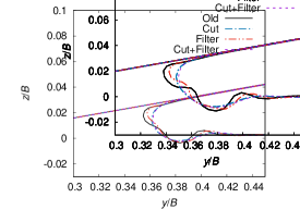
(a) $V/V_{0}=-0.40$

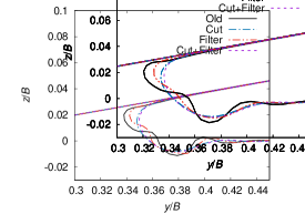
(b) $V/V_{0}=-0.50$

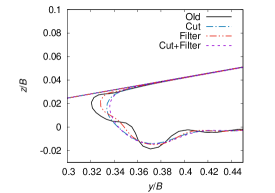
(c) $V/V_{0}=-0.60$

Figure 4: Wedge: close-up view of the free-surface shape in the jet root region at three different time steps during the exit phase.

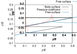
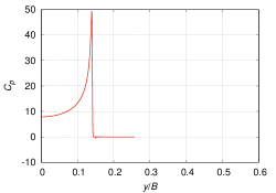
(a) $V/V_{0}=0.80$

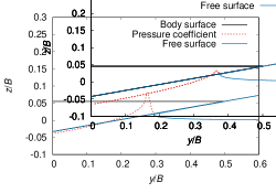
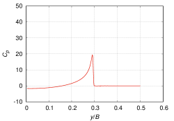
(b) $V/V_{0}=0.50$

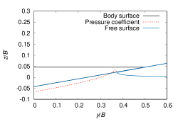
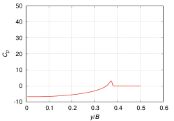
(c) $V/V_{0}=0.20$

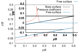
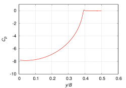
(d) $V/V_{0}=0$

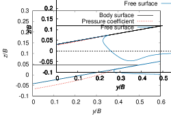
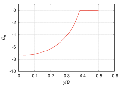
(e) $V/V_{0}=-0.20$

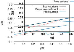
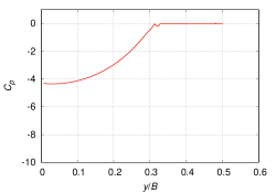
(f) $V/V_{0}=-0.70$

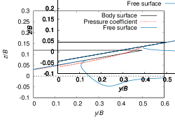
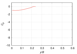
(g) $V/V_{0}=-1.30$

Figure 5: Wedge: free-surface evolution and pressure coefficient distribution

Figure 5 shows the free-surface evolution and the pressure coefficient distribution at different time steps, which is expressed in terms of the ratio between the current velocity $V$ and the initial velocity $V_{0}$. During the entry phase, when the body is going downwards but the velocity is decreasing, the flow rises along the body contour and a thin jet develops and propagates along the body surface. The pressure distribution resembles that in the water entry at constant velocity, presented in[17, 19], but the pressure peak, occurring behind the jet root, progressively diminishes. The same happens to a lesser extent also to the whole pressure distribution, which becomes negative over a large portion of the wetted surface. In the exit phase, when the body is moving upwards and the velocity grows in amplitude, the flow moves in the opposite direction and the pressure remains negative but diminishes in amplitude. At $t^{*}=2$ the body is completely above the still water level and the exit velocity is equal in amplitude to the initial velocity. However, the fluid follows the body and a portion of the body contour is still wet. The exit phase continues for a while until the fluid leaves the body completely. For both phases, the pressure inside the thin jet is essentially negligible. Figure 6 shows the free-surface shape, in proximity of the jet region, obtained in the entry and exit phases at the same body position and for the same velocity absolute value. It can be seen that in the entry phase the wetted length increases faster than it shrinks in the exit phase and this behavior is consistent with what was observed in the CFD results [24].

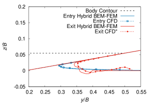
Figure 6: Wedge: free-surface profiles obtained in the entry and exit phases at the same body position and absolute velocity. Results obtained by CFD in [24] are also drawn for comparison.

It is worth noting that the results displayed in Figs. 5 and 6 are obtained by using the filter strategy, but essentially similar results are obtained when using the jet cut off procedure. Figures 7 and 8 provides further details on the pressure behavior, in particular in the entry phase. Figure 7a shows the pressure distribution together with the unsteady term ($\rho\partial\varphi/\partial t$) and the non-linear term of the Bernoulli’s equation, ($\rho u^{2}/2$). Both terms exhibit a sharp growth approaching the spray root, and thus the pressure peak, and a sudden change to a much lower growth rate inside the jet. When reducing the speed, the sharp growth is limited and then the transition to the lower growth rate in the jet appears much milder, as shown in the figure 7b for the non-linear contribution of the pressure. Inside the jet the two contributions balance each other, thus resulting in a zero pressure. Figure 7c shows that, close to the peak, the pressure coincides with the non-linear term of the Bernoulli’s equation, as it happens for the self-similar solution of the case with constant velocity [19]. Although the solution is no longer self-similar, and the pressure peak decreases, such behavior remains valid when the entry velocity decreases (Fig. 7d-e). Furthermore, the pressure peak position, in terms of ratio between the z-coordinate and the current depth $d$, is almost constant over time (Fig.7f).

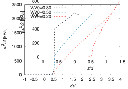
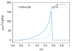
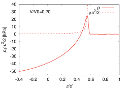
Figure 7: Wedge: pressure details. a) Comparison between the pressure, the non-linear term and the unsteady term of the Bernoulli’s equation at $V/V_{0}=0.80$. b) Non-linear term of the Bernoulli’s equation at three different time steps. c-e) Close-up view of the pressure (solid line) and the non-linear term of the Bernoulli’s equation (dashed line) at $V/V_{0}:c=0.80,d=0.50,e=0.20$. f) Time history of the pressure peak position scaled with the current depth.

In order to better investigate this point, the pressure time histories recorded at three probes are analyzed (Figs. 8a,b). As the jet root approaches the probe, the pressure rises quite sharply and reaches the peak. Due to the decrease of the entry velocity, the pressure peak decreases over time. For each probe, the pressure decreases and becomes negative, during the entry phase ($t^{*}<1$). The pressure remains negative during the exit phase ($t^{*}>1$) but decreases in amplitude until approaching zero. Figure 9 shows the time history of the vertical hydrodynamic force which is non-dimensionalized using the initial velocity $V_{0}$, the width of the wedge $B$ and the water density $\rho$, $F^{*}=F/(\rho V_{0}^{2}B)$. The force increases and is positive in the first part of the entry stage. It decreases and turns negative afterwards; indeed, the positive contribution of the ”slamming term”, which is proportional to the velocity, decreases as the velocity decreases, whereas the effect of the acceleration, which introduces an additional added-mass effect, negative contribution to the force, increases as the wetted area increases. The force remains negative, approaching zero as the body exits from the water. The negative peak in the hydrodynamic loading occurs at the transition between the entry and exit phases, about $t^{*}\simeq 1$, and it is greater than the positive one occurring during the entry phase. The use of different strategies during the exit phase, also in combination, does not affect the results and a quite satisfactory agreement with the CFD [24] and semi-analytical [4] results available in the literature is achieved. Furthermore, for $t^{*}>2$ the force approaches zero slowly, highlighting the capabilities of the numerical model to follow the exit phase until the body has completely emerged, as it happens in the CFD simulations, whereas the semi-analytical model approaches zero earlier showing its limitations in describing the latest stage of the exit phase when the body is above the still water level but the flow is still attached.

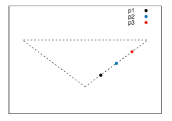
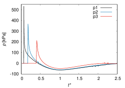
Figure 8: Wedge: a) Pressure sensors position. b) Pressure time history for each sensor

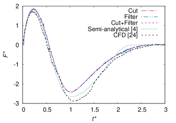
Figure 9: Wedge: non dimensional vertical hydrodynamic force time history.

3.2 Cone

The vertical water entry and exit with imposed motion of a rigid cone with a $15^{\circ}$ deadrise angle, $\beta$, is here presented. The test case is based on the experimental condition used in [8]. In the experiments, the hydrodynamic force acting on the impact body was measured and the use of a transparent mockup and a LED edge-lighting system with a high-speed video camera placed above the mock-up allowed to follow the evolution of the wetted surface during the combined entry and exit event. Starting from the time at which the body touches the water, the cone is moved with a vertical velocity given by the following equations

$$\begin{cases}V(t)=U_{max}\cos(\omega t),\hskip 28.45274ptt\leq T/2\\ V(t)=-U_{max},\hskip 54.06023ptt>T/2\end{cases}$$

where $\omega=U_{max}/H_{max}$ with $U_{max}$ initial, downwards, velocity, $H_{max}$ maximum penetration depth and $T=2\pi H_{max}/U_{max}$. The value of $H_{max}$ is derived from the Wagner’s condition for the wetted surface [8]

$$H_{max}=\frac{c_{max}\pi\tan\beta}{4}$$

where $c_{max}$ is the maximum wetted length. The test case with $U_{max}=0.57$m/s and $c_{max}=200$mm has been chosen. The gravity effects, which could be significant especially in the exit phase [8], are included here. In the previous section, the use of different strategies to improve the numerical stability during the exit phase has been shown. Although the two different approaches provide good results, the combined use of cut and filter strategy is the most preferable. In fact, the jet cut, beside improving the stability, allows to reduce the computational effort whereas the filter strategy can guarantee greater robustness to the solver. Based on the above considerations, the cut+filter strategies are used here, thus managing to stabilize the solution during the exit, as shown in the Figure 10.

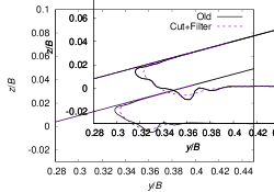
(a) $V/V_{0}=-0.40$

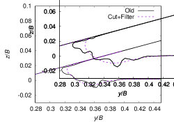
(b) $V/V_{0}=-0.50$

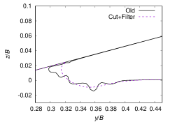
(c) $V/V_{0}=-0.60$

Figure 10: Cone: close-up view of the free-surface shape in the jet root region at three different time steps during the exit phase.

Figure 11 displays the results obtained in terms of free-surface evolution and pressure distribution. Strong similarities with the solution obtained in the wedge case can be observed. During the entry phase the jet rises along the body surface and the pressure decreases, becoming negative. During the exit phase, the flow evolves in the opposite direction and the negative pressure decreases in amplitude. Note that, due to the action of the gravity the pressure returns a little bit positive during the exit phase (see Fig. 11 g). Similarly to the wedge case, the pressure peak decreases but its position, scaled with the current depth, is almost constant in time, and close to the peak the pressure overlaps the value of the non-linear term of the Bernoulli’s equation (Fig. 12). Moreover, the time history of the pressure recordered at different probes is similar (in shape) to what was observed with the wedge (Fig. 13).

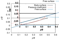
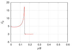
(a) $V/V_{0}=0.90$

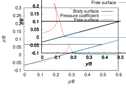
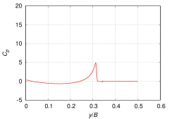
(b) $V/V_{0}=0.50$

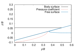
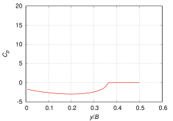
(c) $V/V_{0}=0.10$

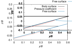
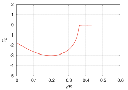
(d) $V/V_{0}=0$

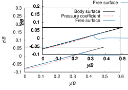
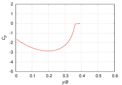
(e) $V/V_{0}=-0.10$

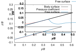
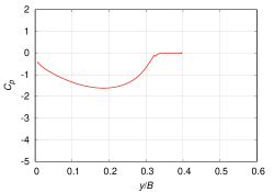
(f) $V/V_{0}=-0.50$

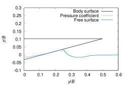
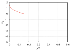
(g) $V/V_{0}=-0.90$

Figure 11: Cone: free-surface evolution and pressure coefficient distribution.

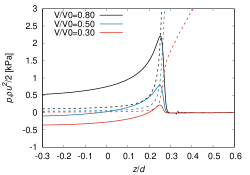
Figure 12: Cone: pressure details. a) Comparison between the pressure (solid line) and the contribution of non-linear term of the Bernoulli’s equation (dashed line) at different time steps. b) Time history of the pressure peak position scaled with the current depth.

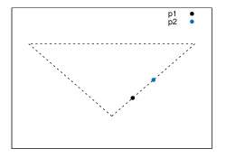
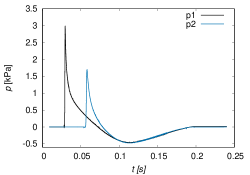
Figure 13: Cone: a) Pressure sensors position. b) Pressure time history for each sensor.

Figure 15 shows the time histories of the hydrodynamic force and of the contact line position, evaluated by following the $y$-coordinate of the jet root, as indicated in Fig.14. The force, computed by pressure integration along the wetted area, is positive in the first part of the entry phase and turns negative afterwards, approaching zero during the exit phase. The negative force peak, occuring at the transition between the entry and exit stages, is higher in amplitude than the maximum force recorded in the entry phase, despite of the action of the gravity. The contact line is maximum at the instant when the body attains its maximum depth, i.e. at the transition between the entry and exit phases, but it is smaller than the maximum expected value $c_{max}$. This is an effect of the presence of the meniscus during the experiments [8] which is considered in the numerical simulation by correcting the body displacement with a parameter $\delta_{z}=3mm$, which practically changes the initial reference vertical position. The asymmetry of the curve with respect to the peak indicates that in the exit phase the wetted surface decreases slower than it increases during the entry phase. The initial step on the curves of the contact line time history obtained with the proposed model, is due to the initial body depth necessary to start the simulation [28]. The results obtained with the proposed fully non-linear model (FNL) are in very good agreement with the experimental data. It is worth noting that in the FNL simulations gravity effects are included. In order to evaluate the role of the gravity, especially during the exit phase, the numerical simulations were conducted with and without gravity. As shown in Fig. 15, the gravity affects both the hydrodynamic force and wetted surface, especially during the exit phase. In Fig. 15b the results obtained with water exit semi-analytical models in [8] are also provided. The first one is the modified von Kármán (MVK), which is an extension to the axisymmetric bodies of the model proposed in [4]. The second one is the extension to axisymmetric bodies and non-constant exit velocity proposed in [8] of the Korobkin model [15]. The semi-analytical models perform much less satisfactorily than the fully non-linear model, presumably because of neglecting the gravity effects. Based on the above considerations, the flexibility of the fully non-linear model seems very helpful for an accurate description of the exit phase.

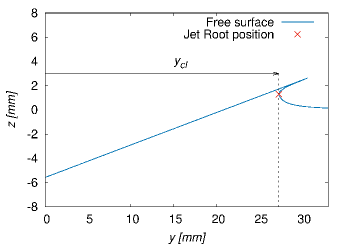
Figure 14: Definition of the contact line

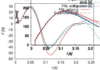
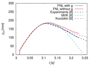
Figure 15: Cone: evolution of the total force acting on the body (a) and of the contact line (b) as a function of time

4 Conclusions

A fully non-linear potential flow model based on the hybrid BEM-FEM approach for the description of combined water entry and exit problems of 2D and axisymmetric bodies has been proposed. The model is an extension of that proposed and validated in [16] and [17] for the water entry with constant velocity applications. In particular, a water exit model that includes two different strategies aimed at improving the stability of the free-surface shape, has been proposed and validated against data available in the literature. Both strategies have been found able to improve the numerical stability of the solution providing similar results in the wedge case, where a very accurate prediction of the free-surface, pressure distribution and vertical hydrodynamic force time histories has been obtained. The combined use of the two strategies both in the cone and the wedge cases has demonstrated further improvement of the stability of the free-surface dynamics. Such combined approach seems the best in terms of computational effort and robustness of the solver.

The detailed information provided by the model also allow an accurate analysis of the pressure distribution along the wetted body portion. In particular, it has been shown that, similarly to what happens in the self-similar solution, the pressure, close to its peak, matches the non-linear term of the Bernoulli’s equation. The results obtained for the cone, for which comparisons with accurate experimental data have been established in terms of hydrodynamic force and wetted area, clearly highlight the strong potential of the proposed model. Furthermore, the role played by the gravity, which is particularly important during the exit phase, as shown in the experiments of [8], has been observed.

As a future work, the model will be extended into a multisectional 2D+t procedure for application to both aircraft ditching and high-speed planing vessels.

Funding

This project has been partly funded from the European Union’s Horizon 2020 Research and Innovation Programme under Grant Agreement No. 724139 (H2020-SARAH: increased SAfety & Robust certification for ditching of Aircrafts & Helicopters).

References

- [1] Battistin, D., Iafrati, A., 2003. A numerical model for hydrodynamics of planning surface. FAST.
- [2] Gropengießer, W., Rung, T., 2016. Computational Modelling of Aircraft Ditching with two-way Fluid-Structure-Interaction. ECCOMAS Congress.
- [3] Martin L., Jacques V., Paul B., 2018. Application of the MLM to evaluate the hydrodynamic loads endured in the event of aircraft ditching. Proceedings of the 6th European Conference on Computational Mechanics (Solids, Structures and Coupled Problems) and 7th European Conference on Computational Fluid Dynamics (ECCM ECFD 2018), Glasgow, UK.
- [4] Tassin, A., Piro, D. J., Korobkin, A. A., Maki, K. J., Cooker, M., 2013. Two-dimensional water entry and exit of a body whose shape varies in time. Journal of Fluids and Structures, 40, 317-336.
- [5] Piro, D. J., Maki, K. J., 2013. Hydroelastic analysis of bodies that enter and exit water. Journal of Fluids and Structures 37, 134-150.
- [6] Semenov, Y. A. , Yoon, B.-S., 2009. Onset of flow separation for the oblique water impact of a wedge. Physics of Fluids 21, 112103.
- [7] Reinhard, M., Korobkin, A. A., Cooker, M. J., 2013. Water entry of a flat elastic plate at high horizontal speed. Journal of Fluid Mechanics 724, 123–153.
- [8] Breton, T., Tassin, A., Jacques, N., 2020. Experimental investigation of the water entry and/or exit of axisymmetric bodies. Journal of Fluid Mechanics 901, A37.
- [9] Wu, Q. G., Ni, B. Y., Bai, X. L., Cui, B., Sun, S. L., 2017. Experimental study on large deformation of free surface during water exit of a sphere. Ocean Engineering 140, 369-376.
- [10] Ni, B. Y., Zhang, A. M., Wu, G. X., 2017. Simulation of complete water exit of a fully-submerged body. FJournal of Fluids and Structures 58, 79-98.
- [11] Ni, B. Y., Wu, G. X., 2017. Numerical simulation of water exit of an initially fully submerged buoyant spheroid in an axisymmetric flow. Fluid Dynamic Research 49, 045511.
- [12] Kaplan, P., 1987. Analysis and prediction of at bottom slamming impact of advanced marine vehicles in waves. International Shipbuilding Progress 34 (391), 44-53.
- [13] Wagner, H., 1932. Über Stoß- und Gleitvorgänge an der Oberfäche von Flüssigkeiten. ZAMM 12, 193-215.
- [14] Korobkin, A. A., 2013. A linearized model of water exit. Journal of Fluid Mechanics 737, 368-386.
- [15] Korobkin, A. A., Khabakhpasheva, T. Maki, K. J., 2017. Hydrodynamic forces in water exit problems. Journal of Fluids and Structures 69, 16-33.
- [16] Battistin, D., Iafrati, A., 2003. Hydrodynamic loads during water entry of two-dimensional and axisymmetric bodies. Journal of Fluids and Structures, 17, 643-664.
- [17] Battistin, D., Iafrati, A., 2004. A numerical model for the jet flow generated by water impact. Journal of Engineering Mathematics, 48, 353-374.
- [18] Longuet-Higgins, M. S., Cokelet, E. D., 1976. The deformation of steep surface waves on water. I. A numerical method. Proc R Soc London, A350, 1-26.
- [19] Zhao, R., Faltinsen, O. M., 1993. Water entry of two-dimensional bodies. Journal of Fluid Mechanics, 246, 593–612.
- [20] Zhao, R., Faltinsen, O. M., Aarsnes, J. V., 1996. Water entry of arbitrary two-dimensional sections with and without flow separation. In: Proceedings of twenty-first symposium on naval hydrodynamics, Trondheim, Norway.
- [21] Iafrati, A., Battistin, D., 2003. Hydrodynamics of water entry in presence of flow separation from chines. Proceedings of the 8th International Conference on Numerical Ship Hydrodynamics, Busan, Korea.
- [22] Baarholm, R., Faltinsen, O. M., 2004. Wave impact underneath horizontal decks. Journal of Marine Science Technology, 9, 1-13.
- [23] Dold, J. W., 1992. An Efficient Surface-Integral Algorithm Applied to Unsteady Gravity Waves. Journal of Computational Physics, 103, 90-115.
- [24] Piro, D. J., Maki, K. J., 2011. Hydroelastic wedge entry and exit. Proceedings of 11th International Conference on Fast Sea Transportation, Honolulu, HI, USA.
- [25] Sun, H., Faltinsen, O. M., 2006. Water impact of horizontal circular cylinders and cylindrical shells. Applied Ocean Research, 28, 299-311.
- [26] Iafrati, A., Grizzi, S., 2019. Cavitation and ventilation modalities during ditching. Physics of Fluids, 31, 052101.
- [27] Greenhow, M., 1987. Wedge entry into initially calm water. Applied Ocean Research, 9, 214–223.
- [28] Iafrati, A., Carcaterra, A., Ciappi, E., Campana, E. F., 2000. Hydroelastic analysis of a simple oscillator impacting the free surface. Journal of Ship Research 44, 278–289.