Compound matrices in systems and control theory

Abstract

The multiplicative and additive compounds of a matrix play an important role in several fields of mathematics including geometry, multi-linear algebra, combinatorics, and the analysis of nonlinear time-varying dynamical systems. There is a growing interest in applications of these compounds, and their generalizations, in systems and control theory. This tutorial paper provides a gentle introduction to these topics with an emphasis on the geometric interpretation of the compounds, and surveys some of their recent applications.

I Introduction

Let $A\in\mathbb{R}^{n\times n}$. Fix $k\in\{1,\dots,n\}$. The $k$-multiplicative and $k$-additive compounds of $A$ play an important role in several fields of applied mathematics. Recently, there is a growing interest in the applications of these compounds, and their generalizations, in systems and control theory (see, e.g. [43, 42, 21, 1, 5, 28, 44, 40, 2, 41, 13, 16, 14, 17, 15]).

This tutorial paper reviews the $k$-compounds, focusing on their geometric interpretations, and surveys some of their recent applications in systems and control theory, including $k$-positive systems, $k$-cooperative systems, and $k$-contracting systems.

The results described here are known, albeit never collected in a single paper. The only exception is the new generalization principle described in Section V.

We use standard notation. For a set $S$, $\operatorname{int}(S)$ is the interior of $S$. For scalars $\lambda_{i}$, $i\in\{1,\dots,n\}$, $\operatorname{diag}(\lambda_{1},\dots,\lambda_{n})$ is the $n\times n$ diagonal matrix with diagonal entries $\lambda_{i}$. Column vectors [matrices] are denoted by small [capital] letters. For a matrix $A$, $A^{T}$ is the transpose of $A$. For a square matrix $B$, $\operatorname{tr}(B)$ [$\det(B)$] is the trace [determinant] of $B$. $B$ is called Metzler if all its off-diagonal entries are non-negative. The positive orthant in $\mathbb{R}^{n}$ is $\mathbb{R}^{n}_{+}=\{x\in\mathbb{R}^{n}:x_{i}\geq 0,\;i=1,\dots,n\}$.

II Geometric motivation

$k$-compound matrices provide information on the evolution of $k$-dimensional polygons subject to a linear time-varying dynamics. To explain this in a simple setting, consider the LTI system:

$$\dot{x}=\operatorname{diag}(\lambda_{1},\lambda_{2},\lambda_{3})x,$$ (1)

with $\lambda_{i}\in\mathbb{R}$ and $x:\mathbb{R}_{+}\to\mathbb{R}^{3}$. Let $e^{i}$, $i=1,2,3$, denote the $i$th canonical vector in $\mathbb{R}^{3}$. For $x(0)=e^{i}$ we have $x(t)=\exp(\lambda_{i}t)x(0)$. Thus, $\exp(\lambda_{i}t)$ describes the rate of evolution of the line $e^{i}$ subject to (1). What about 2D areas? Let $S\subset\mathbb{R}^{3}$ denote the square generated by $e^{i}$ and $e^{j}$, with $i\not=j$. Then $S(t):=x(t,S)$ is the rectangle generated by $\exp(\lambda_{i}t)e^{i}$ and $\exp(\lambda_{j}t)e^{j}$, so the area of $S(t)$ is $\exp((\lambda_{i}+\lambda_{j})t)$. Similarly, if $B\subset\mathbb{R}^{3}$ is the 3D box generated by $e^{1},e^{2}$, and $e^{3}$ then the volume of $B(t):=x(t,B)$ is $\exp((\lambda_{1}+\lambda_{2}+\lambda_{3})t)$ (see Fig. 1).

Since $\exp(At)=\operatorname{diag}(\exp(\lambda_{1}t),\exp(\lambda_{2}t),\exp(\lambda_{3}t))$, this discussion suggests that it may be useful to have a $3\times 3$ matrix whose eigenvalues are the sums of any two eigenvalues of $\exp(At)$, and a $1\times 1$ matrix whose eigenvalue is the sum of the three eigenvalues of $\exp(At)$. With this geometric motivation in mind, we turn to recall the notions of the multiplicative and additive compounds of a matrix. For more details and proofs, see e.g. [11, Ch. 6][33].

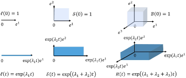
Figure 1: The evolution of lines, areas, and volumes under the the LTI (1).

III Compound Matrices

Let $A\in\mathbb{C}^{n\times m}$. Fix $k\in\{1,\dots,\min\{n,m\}\}$. Let $Q(k,n)$ denote the set of increasing sequences of $k$ integers in $\{1,\dots,n\}$, ordered lexicographically. For example,

$$Q(2,3)=\{\{1,2\},\{1,3\},\{2,3\}\}.$$

For $\alpha\in Q(k,n),\beta\in Q(k,m)$, let $A[\alpha|\beta]$ denote the $k\times k$ submtarix obtained by taking the entries of $A$ in the rows indexed by $\alpha$ and the columns indexed by $\beta$. For example

$$A[\{1,2\}|\{2,3\}]=\begin{bmatrix}a_{12}&a_{13}\\ a_{22}&a_{23}\end{bmatrix}.$$

The minor of $A$ corresponding to $\alpha,\beta$ is $A(\alpha|\beta):=\det(A[\alpha|\beta])$. For example, $Q(n,n)$ includes the single set $\alpha=\{1,\dots,n\}$ and $A(\alpha|\alpha)=\det(A)$.

Definition 1

Let $A\in C^{n\times m}$ and fix $k\in\{1,\dots,\min\{n,m\}\}$. The $k$-multiplicative compound of $A$, denoted $A^{(k)}$, is the $\binom{n}{k}\times\binom{m}{k}$ matrix that contains all the $k$-order minors of $A$ ordered lexicographically.

For example, if $n=m=3$ and $k=2$ then

$$A^{(2)}=\begin{bmatrix}A(\{12\}|\{12\})&A(\{12\}|\{13\})&A(\{12\}|\{23\})\\ A(\{13\}|\{12\})&A(\{13\}|\{13\})&A(\{13\}|\{23\})\\ A(\{23\}|\{12\})&A(\{23\}|\{13\})&A(\{23\}|\{23\})\end{bmatrix}.$$

In particular, Definition 1 implies that $A^{(1)}=A$, and if $n=m$ then $A^{(n)}=\det(A)$.

Let $A\in\mathbb{C}^{n\times m},\;B\in\mathbb{C}^{m\times p}$. The Cauchy-Binet Formula (see e.g. [12]) asserts that for any $k\in\{1,\dots,\min\{n,m,p\}\}$,

$$(AB)^{(k)}=A^{(k)}B^{(k)}.$$ (2)

Hence the term multiplicative compound. Note that for $n=m=p$, Eq. (2) with $k=n$ reduces to the familiar formula $\det(AB)=\det(A)\det(B)$.

Let $I_{s}$ denote the $s\times s$ identity matrix. Definition 1 implies that $I_{n}^{(k)}=I_{r}$, where $r:=\binom{n}{k}$. Hence, if $A\in\mathbb{R}^{n\times n}$ is non-singular then $(AA^{-1})^{(k)}=I_{r}$ and combining this with (2) yields $(A^{-1})^{(k)}=(A^{(k)})^{-1}$. In particular, if $A$ is non-singular then so is $A^{(k)}$.

The $k$-multiplicative compound has an important spectral property. For $A\in\mathbb{C}^{n\times n}$, let $\lambda_{i}$, $i=1,\dots,n$, denote the eigenvalues of $A$. Then the eigenvalues of $A^{(k)}$ are all the products

$$\prod_{\ell=1}^{k}\lambda_{i_{\ell}},\text{ with }1\leq i_{1}<i_{2}<\dots<i_{k}\leq n.$$ (3)

For example, suppose that $n=3$ and $A=\begin{bmatrix}a_{11}&a_{12}&a_{13}\\ 0&a_{22}&a_{23}\\ 0&0&a_{33}\end{bmatrix}.$ Then a calculation gives

$$A^{(2)}=\begin{bmatrix}a_{11}a_{22}&a_{11}a_{23}&a_{12}a_{23}-a_{13}a_{22}\\ 0&a_{11}a_{33}&a_{12}a_{33}\\ 0&0&a_{22}a_{33}\end{bmatrix},$$

so, clearly, the eigenvalues of $A^{(2)}$ are of the form (3).

Definition 2

Let $A\in\mathbb{C}^{n\times n}$. The $k$-additive compound matrix of $A$ is defined by:

$$A^{[k]}:=\frac{d}{d\epsilon}(I+\epsilon A)^{(k)}|_{\epsilon=0}.$$

Note that this implies that $A^{[k]}=\frac{d}{d\epsilon}(\exp(A\epsilon))^{(k)}|_{\epsilon=0}$, and also that

$$(I+\epsilon A)^{(k)}=I+\epsilon A^{[k]}+o(\epsilon),$$ (4)

In other words, $A^{[k]}$ is the first-order term in the Taylor expansion of $(I+\epsilon A)^{(k)}$.

Let $\lambda_{i}$, $i=1,\dots,n$, denote the eigenvalues of $A$. Then the eigenvalues of $(I+\epsilon A)^{(k)}$ are the products $\prod_{\ell=1}^{k}(1+\epsilon\lambda_{i_{\ell}})$, and (4) implies that the eigenvalues of $A^{[k]}$ are all the sums

$$\sum_{\ell=1}^{k}\lambda_{i_{\ell}},\text{ with }1\leq i_{1}<i_{2}<\dots<i_{k}\leq n.$$

Another important implication of the definitions above is that for any $A,B\in\mathbb{C}^{n\times n}$ we have

$$(A+B)^{[k]}=A^{[k]}+B^{[k]}.$$

This justifies the term additive compound. Moreover, the mapping $A\to A^{[k]}$ is linear.

The following result gives a useful explicit formula for $A^{[k]}$ in terms of the entries $a_{ij}$ of $A$. Recall that any entry of $A^{(k)}$ is a minor $A(\alpha|\beta)$. Thus, it is natural to index the entries of $A^{(k)}$ and $A^{[k]}$ using $\alpha,\beta\in Q(k,n)$.

Proposition 1

Fix $\alpha,\beta\in Q(k,n)$ and let $\alpha=\{i_{1},\dots,i_{k}\}$ and $\beta=\{j_{1},\dots,j_{k}\}$. Then the entry of $A^{[k]}$ corresponding to $(\alpha,\beta)$ is equal to:

1. $\sum_{\ell=1}^{k}a_{i_{\ell}i_{\ell}}$, if $i_{\ell}=j_{\ell}$ for all $\ell\in\{1,\ldots,k\}$;

2. $(-1)^{\ell+m}a_{i_{\ell}j_{m}}$, if all the indices in $\alpha$ and $\beta$ agree, except for a single index $i_{\ell}\neq j_{m}$; and

3. $0$, otherwise.

Example 1

For $A\in\mathbb{R}^{4\times 4}$ and $k=3$, Prop. 1 yields

$$A^{[3]}=\left[\scalebox{0.67}{\mbox{$\displaystyle\begin{array}[]{ccccccc}a_{11}+a_{22}+a_{33}&a_{34}&-a_{24}&a_{14}\\ a_{43}&a_{11}+a_{22}+a_{44}&a_{23}&-a_{13}\\ -a_{42}&a_{32}&a_{11}+a_{33}+a_{44}&a_{12}\\ a_{41}&-a_{31}&a_{21}&a_{22}+a_{33}+a_{44}\end{array}$}}\right].$$

The entry in the second row and fourth column of $A^{[3]}$ corresponds to $(\alpha|\beta)=(\{1,2,4\}|\{2,3,4\})$. As $\alpha$ and $\beta$ agree in all indices except for the index $i_{1}=1$ and $j_{2}=3$, this entry is equal to $(-1)^{1+2}a_{13}=-a_{13}$.

Note that Prop. 1 implies in particular that $A^{[n]}=\operatorname{tr}(A)$.

The next section describes applications of compound matrices for dynamical systems described by ODEs. For more details and proofs, see [33, 29].

IV Compound Matrices and ODEs

Fix an interval $[a,b]\in\mathbb{R}$. Let $A:[a,b]\to\mathbb{R}^{n\times n}$ be a continuous matrix function, and consider the LTV system:

$$\dot{x}(t)=A(t)x(t),\quad x(a)=x_{0}.$$ (5)

The solution is given by $x(t)=\Phi(t,a)x(a)$, where $\Phi(t,a)$ is the solution at time $t$ of the matrix differential equation

$$\dot{\Phi}(s)=A(s)\Phi(s),\quad\Phi(a)=I_{n}.$$ (6)

Fix $k\in\{1,\dots,n\}$ and let $r:=\binom{n}{k}$. A natural question is: how do the $k$-order minors of $\Phi(t)$ evolve in time? The next result provides a beautiful formula for the evolution of $\Phi^{(k)}(t):=(\Phi(t))^{(k)}$.

Proposition 2

If $\Phi$ satisfies (6) then

$$\frac{d}{dt}\Phi^{(k)}(t)=A^{[k]}(t)\Phi^{(k)}(t),\quad\Phi^{(k)}(a)=I_{r},$$ (7)

where $A^{[k]}(t):=(A(t))^{[k]}$.

Thus, the $k\times k$ minors of $\Phi$ also satisfy an LTV. In particular, if $A(t)\equiv A$ and $a=0$ then $\Phi(t)=\exp(At)$ so $\Phi^{(k)}(t)=(\exp(At))^{(k)}$ and (7) gives

$$(\exp(At))^{(k)}=\exp(A^{[k]}t).$$

Note also that for $k=n$, Prop. 2 yields

$$\frac{d}{dt}\det(\Phi(t))=\operatorname{tr}(A(t))\det(\Phi(t)),$$

which is the Abel-Jacobi-Liouville identity.

Roughly speaking, Prop. 2 implies that under the LTV dynamics (5), $k$-dimensional polygons evolve according to the dynamics (7).

We now turn to consider the nonlinear system:

$$\dot{x}(t)=f(t,x).$$ (8)

For the sake of simplicity, we assume that the initial time is zero, and that the system admits a convex and compact state-space $\Omega$. We also assume that $f\in C^{1}$. The Jacobian of the vector field $f$ is $J(t,x):=\frac{\partial}{\partial x}f(t,x)$.

Compound matrices can be used to analyze (8) by using an LTV called the variational equation associated with (8). To define it, fix $a,b\in\Omega$. Let $z(t):=x(t,a)-x(t,b)$, and for $s\in[0,1]$, let $\gamma(s):=sx(t,a)+(1-s)x(t,b)$, i.e. the line connecting $x(t,a)$ and $x(t,b)$. Then

$$\dot{z}(t) =f(t,x(t,a))-f(t,x(t,b))$$

$$=\int_{0}^{1}\frac{\partial}{\partial s}f(t,\gamma(s))\mathop{}\!\mathrm{d}s,$$

and this gives the variational equation:

$$\dot{z}(t)=A^{ab}(t)z(t),$$ (9)

where

$$A^{ab}(t):=\int_{0}^{1}J(t,\gamma(s))\mathop{}\!\mathrm{d}s.$$ (10)

We can use the results above to describe a powerful approach for deriving useful “$k$-generalizations” of important classes of dynamical systems including cooperative systems [36], contracting systems [3, 24], and diagonally stable systems [20].

V $k$-generalizations of dynamical systems

Consider the LTV (5). Suppose that $A(t)$ satisfies a specific property, e.g. property may be that $A(t)$ is Metzler for all $t$ (so the LTV is positive) or that $\mu(A(t))\leq-\eta<0$ for all $t$, where $\mu:\mathbb{R}^{n\times n}\to\mathbb{R}$ is a matrix measure (so the LTV is contracting). Fix $k\in\{1,\dots,n\}$. We say that the LTV satisfies $k$-property if $A^{[k]}$ (rather than $A$) satisfies property. For example, the LTV is $k$-positive if $A^{[k]}(t)$ is Metzler for all $t$; the LTV is $k$-contracting if $\mu(A^{[k]}(t))\leq-\eta<0$ for all $t$, and so on.

This generalization approach makes sense for two reasons. First, when $k=1$, $A^{[k]}$ reduces to $A^{[1]}=A$, so $k$-property is clearly a generalization of property. Second, we know that $A^{[k]}$ has a clear geometric meaning, as it describes the evolution of $k$-dimensional polygons along the dynamics.

The same idea can be applied to the nonlinear system (8) using the variational equation (9). For example, if $\mu(J(t,x))\leq-\eta<0$ for all $t\geq 0$ and $x\in\Omega$ then (8) is contracting: the distance between any two solutions (in the norm that induced $\mu$) decays at an exponential rate. If we replace this by the condition $\mu(J^{[k]}(t,x))\leq-\eta<0$ for all $t\geq 0$ and $x\in\Omega$ then (8) is called $k$-contracting. Roughly speaking, this means that the volume of $k$-dimensional polygons decays to zero exponentially along the flow of the nonlinear system. We now turn to describe several such $k$-generalizations.

VI $k$-contracting systems

$k$-contracting systems were introduced in [42] (see also the unpublished preprint [26] for some preliminary ideas). For $k=1$ these reduce to contracting systems. This generalization was motivated in part by the seminal work of Muldowney [29] who considered nonlinear systems that, in the new terminology, are $2$-contracting. He derived several interesting results for time-invariant $2$-contracting systems. For example, every bounded trajectory of a time-invariant, nonlinear, $2$-contracting system converges to an equilibrium (but, unlike in the case of contracting systems, the equilibrium is not necessarily unique).

For the sake of simplicity, we introduce the ideas in the context of an LTV system. The analysis of nonlinear systems is based on assuming that their variational equation is a $k$-contracting LTV.

Recall that a vector norm $|\cdot|:\mathbb{R}^{n}\to\mathbb{R}_{+}$ induces a matrix norm $||\cdot||:\mathbb{R}^{n\times n}\to\mathbb{R}_{+}$ by:

$$||A||:=\max_{|x|=1}|Ax|,$$

and a matrix measure $\mu(\cdot):\mathbb{R}^{n\times n}\to\mathbb{R}$ by:

$$\mu(A):=\lim_{\epsilon\downarrow 0}\frac{||I+\epsilon A||-1}{\epsilon}.$$

For $p\in\{1,2,\infty\}$, let $|\cdot|_{p}:\mathbb{R}^{n}\to\mathbb{R}_{+}$ denote the $L_{p}$ vector norm, that is, $|x|_{1}:=\sum_{i=1}^{n}|x_{i}|$, $|x|_{2}:=\sqrt{x^{T}x}$, and $|x|_{\infty}:=\max_{i\in\{1,\dots,n\}}|x_{i}|$. The induced matrix measures are [39]:

$$\mu_{1}(A) =\max_{j\in\{1,\dots,n\}}(a_{jj}+\sum_{\begin{subarray}{c}i=1\\ i\neq j\end{subarray}}^{n}|a_{ij}|),$$ (11)

$$\mu_{2}(A) =\lambda_{1}({A+A^{T}})/2,$$

$$\mu_{\infty}(A) =\max_{i\in\{1,\dots,n\}}(a_{ii}+\sum_{\begin{subarray}{c}j=1\\ j\neq i\end{subarray}}^{n}|a_{ij}|),$$

where $\lambda_{i}(S)$ denotes the $i$-th largest eigenvalue of the symmetric matrix $S$, that is,

$$\lambda_{1}(S)\geq\lambda_{2}(S)\geq\cdots\geq\lambda_{n}(S).$$

Definition 3

The LTV (5) is called $k$-contracting with respect to (w.r.t.) the norm $|\cdot|$ if

$$\mu(A^{[k]}(t))\leq-\eta<0\text{ for all }t\geq 0,$$ (12)

where $\mu$ is the matrix measure induced by $|\cdot|$.

Note that for $k=1$ condition (12) reduces to the standard infinitesimal condition for contraction [3]. For the $L_{p}$ norms, with $p\in\{1,2,\infty\}$, this condition is easy to check using the explicit expressions for $\mu_{1}$, $\mu_{2}$, and $\mu_{\infty}$. This carries over to $k$-contraction, as combining Prop. 1 with (11) gives [29]:

$$\mu_{1}(A^{[k]}) =\max_{\alpha\in Q(k,n)}(\sum_{p=1}^{k}a_{\alpha_{p},\alpha_{p}}+\sum_{\begin{subarray}{c}j\notin\alpha\end{subarray}}(|a_{j,\alpha_{1}}|+\cdots+|a_{j,\alpha_{k}}|)),$$

$$\mu_{2}(A^{[k]}) =\sum_{i=1}^{k}\lambda_{i}({A+A^{T}})/2,$$

$$\mu_{\infty}(A^{[k]}) =\max_{\alpha\in Q(k,n)}(\sum_{p=1}^{k}a_{\alpha_{p},\alpha_{p}}+\sum_{\begin{subarray}{c}j\notin\alpha\end{subarray}}(|a_{\alpha_{1},j}|+\cdots+|a_{\alpha_{k},j}|)).$$

For $k=n$, $A^{[n]}$ is the scalar $\operatorname{tr}(A)$, so condition (12) becomes $\operatorname{tr}(A(t))\leq-\eta<0$ for all $t\geq 0$.

Combining Coppel’s inequality [6] with (7) yields the following result.

Proposition 3

If the LTV (5) is $k$-contracting then

$$||\Phi^{(k)}(t)||\leq\exp(-\eta t)||\Phi^{(k)}(0)||=\exp(-\eta t)$$

for all $t\geq 0$.

Geometrically, this means that under the LTV dynamics the volume of $k$-dimensional polygons converges to zero exponentially. The next example illustrates this.

Example 2

Consider the LTV (5) with $n=2$ and $A(t)=\begin{bmatrix}-1&0\\ -2\cos(t)&0\end{bmatrix}.$ The corresponding transition matrix is: $\Phi(t)=\begin{bmatrix}\exp(-t)&0\\ -1+\exp(-t)(\cos(t)-\sin(t))&1\end{bmatrix}.$ This implies that the LTV is uniformly stable, and that for any $x(0)\in\mathbb{R}^{2}$ we have

$$\lim_{t\to\infty}x(t,x(0))=\begin{bmatrix}0\\ x_{2}(0)-x_{1}(0)\end{bmatrix}.$$

The LTV is not contracting, w.r.t. any norm, as there is more than a single equilibrium. However, $A^{[2]}(t)=\operatorname{tr}(A(t))\equiv-1$, so the system is $2$-contracting. Let $S\subset\mathbb{R}^{2}$ denote the unit square, and let $S(t):=x(t,S)$, that is, the evolution at time $t$ of the unit square under the dynamics. Fig. 2 depicts $S(t)+2t$ for several values of $t$, where the shift by $2t$ is for the sake of clarity. It may be seen that the area of $S(t)$ decays with $t$, and that $S(t)$ converges to a line.

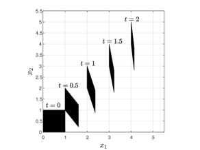
Figure 2: Evolution of the unit square in Example 2.

As noted above, time-invariant $2$-contracting systems have a “well-odered” asymptotic behaviour [29, 23], and this has been used to derive a global analysis of important models from epidemiology (see, e.g. [22]). A recent paper [30] extended some of these results to systems that are not necessarily $2$-contracting, but can be represented as the serial interconnections of $k$-contracting systems, with $k\in\{1,2\}$.

VII $\alpha$-compounds and $\alpha$-contracting systems

A recent paper [44] defined a generalizations called the $\alpha$-multiplicative compound and $\alpha$-additive compound of a matrix, where $\alpha$ is a real number. Let $A\in\mathbb{C}^{n\times n}$ be non-singular. If $\alpha=k+s$, where $k\in\{1,\dots,n-1\}$ and $s\in(0,1)$ then the $\alpha$-multiplicative of $A$ is defined by:

$$A^{(\alpha)}:=(A^{(k)})^{1-s}\otimes(A^{(k+1)})^{s},$$

where $\otimes$ denotes the Kronecker product. This is a kind of “multiplicative interpolation” between $A^{(k)}$ and $A^{(k+1)}$. For example, $A^{(2.1)}=(A^{(2)})^{0.9}\otimes(A^{(3)})^{0.1}$. The $\alpha$-additive compound is defined just like the $k$-additive compound, that is,

$$A^{[\alpha]}:=\frac{d}{d\epsilon}(I+\epsilon A)^{(\alpha)}|_{\epsilon=0},$$

and it was shown in [44] that this yields

$$A^{[\alpha]}=((1-s)A^{[k]})\oplus(sA^{[k+1]}),$$

where $\oplus$ denotes the Kronecker sum.

The system (8) is called $\alpha$-contracting w.r.t. the norm $|\cdot|$ if

$$\mu(J^{[\alpha]}(t,x))\leq-\eta<0,$$ (13)

for all $t\geq 0$ and all $x$ in the state space [44].

Using this notion, it is possible to restate the seminal results of Douady and Oesterlé [7] as follows.

Theorem 1

[44] Suppose that (8) is $\alpha$-contracting for some $\alpha\in[1,n]$. Then any compact and strongly invariant set of the dynamics has a Hausdorff dimension smaller than $\alpha$.

Roughly speaking, the dynamics contracts sets with a larger Hausdorff dimension.

The next example, adapted from [44], shows how these notions can be used to “de-chaotify” a nonlinear dynamical system by feedback.

Example 3

Thomas’ cyclically symmetric attractor [38, 4] is a popular example for a chaotic system. It is described by:

$$\dot{x}_{1}= \sin(x_{2})-bx_{1},$$

$$\dot{x}_{2}= \sin(x_{3})-bx_{2},$$ (14)

$$\dot{x}_{3}= \sin(x_{1})-bx_{3},$$

where $b>0$ is the dissipation constant. The convex and compact set $D:=\{x\in\mathbb{R}^{3}:b|x|_{\infty}\leq 1\}$ is an invariant set of the dynamics.

Fig. 3 depicts the solution of the system emanating from $\begin{bmatrix}1&-2&1\end{bmatrix}^{T}$ for $b=0.1$. Note the symmetric strange attractor.

The Jacobian $J_{f}$ of the vector field in (3) is

$$J_{f}(x)=\begin{bmatrix}-b&\cos(x_{2})&0\\ 0&-b&\cos(x_{3})\\ \cos(x_{1})&0&-b\end{bmatrix},$$

and thus

$$J_{f}^{[2]}(x)=\begin{bmatrix}-2b&\cos(x_{3})&0\\ 0&-2b&\cos(x_{2})\\ -\cos(x_{1})&0&-2b\end{bmatrix},$$

and $J_{f}^{[3]}=\operatorname{trace}(J(x))=-3b$. Since $b>0$, this implies that the system is $3$-contracting w.r.t. any norm. Let $\alpha=2+s$, with $s\in(0,1)$. Then

$$J_{f}^{[\alpha]}(x)=(1-s)J_{f}^{[2]}(x)\oplus sJ_{f}^{[3]}(x)$$

$$=\begin{bmatrix}-(2+s)b&(1-s)\cos(x_{3})&0\\ 0&-(2+s)b&(1-s)\cos(x_{2})\\ -(1-s)\cos(x_{1})&0&-(2+s)b\\ \end{bmatrix}.$$

This implies that

$$\mu_{1}(J_{f}^{[\alpha]}(x))\leq 1-2b-s(b+1),\text{ for all }x\in D.$$

We conclude that for any $b\in(0,1/2)$ the system is $(2+s)$-contracting for any $s>\frac{1-2b}{1+b}$.

We now show how $\alpha$-contarction can be used to design a partial-state controller for the system guaranteeing that the closed-loop system has a “well-ordered” behaviour. Suppose that the closed-loop system is:

$$\dot{x}=f(x)+g(x),$$

where $g$ is the controller. Let $\alpha=2+s$, with $s\in(0,1)$. The Jacobian of the closed-loop system is $J_{cl}:=J_{f}+J_{g}$, so

$$\mu_{1}(J_{cl}^{[\alpha]}) =\mu_{1}(J_{f}^{[\alpha]}+J_{g}^{[\alpha]})$$

$$\leq\mu_{1}(J_{f}^{[\alpha]})+\mu_{1}(J_{g}^{[\alpha]})$$

$$\leq 1-2b-s(b+1)+\mu_{1}(J_{g}^{[\alpha]}).$$

This implies that the closed-loop system is $\alpha$-contracting if

$$\mu_{1}(J^{[\alpha]}_{g}(x))<s(b+1)+2b-1\text{ for all }x\in D.$$ (15)

Consider, for example, the controller $g(x_{1},x_{2})=c\operatorname{diag}(1,1,0)x$, with gain $c<0$. Then $J_{g}^{[\alpha]}=c\operatorname{diag}(2,1+s,1+s)$ and for any $c<0$ condition (15) becomes

$$(1+s)c<s(b+1)+2b-1.$$ (16)

This provides a simple recipe for determining the gain $c$ so that the closed-loop system is $(2+s)$-contracting. For example, when $s\to 0$, Eq. (16) yields $c<2b-1$, and this guarantees that the closed-loop system is $2$-contracting. Recall that in a $2$-contracting system every nonempty omega limit set is a single equilibrium, thus ruling out chaotic attractors and even non-trivial limit cycles [23]. Fig. 4 depicts the behaviour of the closed-loop system with $b=0.1$ and $c=2b-1.1$. The closed-loop system is thus $2$-contracting, and as expected every solution converges to an equilibrium.

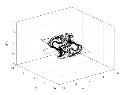
Figure 3: A trajectory emanating from $x(0)=\begin{bmatrix}1&-2&1\end{bmatrix}^{T}$.

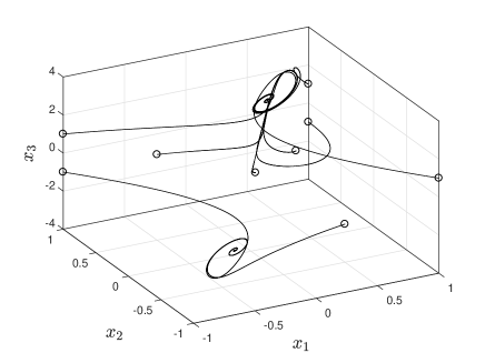
Figure 4: Several trajectories of the closed-loop system. The circles denote the initial conditions of the trajectories.

VIII $k$-positive systems

Ref. [40] introduced the notions of $k$-positive and $k$-cooperative systems. The LTV (5) is called $k$-positive if $A^{[k]}(t)$ is Metzler for all $t$. For $k=1$ this reduces to requiring that $A(t)$ is Metzler for all $t$. In this case the system is positive i.e. the flow maps $\mathbb{R}^{n}_{+}$ to $\mathbb{R}^{n}_{+}$ (and also $\mathbb{R}^{n}_{-}:=-\mathbb{R}^{n}_{+}$ to $\mathbb{R}^{n}_{-}$) [10]. In other words, the flow maps the set of vectors with zero sign variations to itself.

$k$-positive systems map the set of vectors with up to $k-1$ sign variations to itself. To explain this, we recall some definitions and results from the theory of totally positive (TP) matrices, that is, matrices whose minors are all positive [9, 31].

For a vector $x\in\mathbb{R}^{n}\setminus\{0\}$, let $s^{-}(x)$ denote the number of sign variations in $x$ after deleting all its zero entries. For example, $s^{-}(\begin{bmatrix}-1&0&0&2&-3\end{bmatrix}^{T})=2$. We define $s^{-}(0):=0$. For a vector $x\in\mathbb{R}^{n}$, let $s^{+}(x)$ denote the maximal possible number of sign variations in $x$ after setting every zero entry in $x$ to either $-1$ or $+1$. For example, $s^{+}(\begin{bmatrix}-1&0&0&2&-3\end{bmatrix}^{T})=4$. These definitions imply that $0\leq s^{-}(x)\leq s^{+}(x)\leq n-1$, for all $x\in\mathbb{R}^{n}.$

For any $k\in\{1,\dots,n\}$, define the sets

$$P_{-}^{k} :=\{z\in\mathbb{R}^{n}:\;s^{-}(z)\leq k-1\},$$

$$P_{+}^{k} :=\{z\in\mathbb{R}^{n}:\;s^{+}(z)\leq k-1\}.$$ (17)

In other words, these are the sets of all vectors with up to $k-1$ sign variations. Then $P_{-}^{k}$ is closed, and it can be shown that $P_{+}^{k}=\operatorname{int}(P_{-}^{k})$. For example,

$$P_{-}^{1}=\mathbb{R}_{+}^{n}\cup\mathbb{R}_{-}^{n},\;\;\;P_{+}^{1}=\operatorname{int}(\mathbb{R}_{+}^{n})\cup\operatorname{int}(\mathbb{R}_{-}^{n}).$$

Definition 4

The LTV (5) is called $k$-positive on an interval $[a,b]$ if for any $a<t_{0}<b$,

$$x(t_{0})\in P^{k}_{-}\implies x(t,x(t_{0}))\in P^{k}_{-}\text{ for all }t_{0}\leq t<b,$$

and is called strongly $k$-positive if

$$x(t_{0})\in P^{k}_{-}\implies x(t,x(t_{0}))\in P^{k}_{+}\text{ for all }t_{0}<t<b.$$

In other words, the sets of up to $k-1$ sign variations are invariant sets of the dynamics.

An important property of TP matrices is their sign variation diminishing property: if $A\in\mathbb{R}^{n\times n}$ is TP and $x\in\mathbb{R}^{n}\setminus\{0\}$ then $s^{+}(Ax)\leq s^{-}(x)$. In other words, multiplying a vector by a TP matrix can only decrease the number of sign variations. For our purposes, we need a more specialized result. Recall that $A\in\mathbb{R}^{n\times n}$ is called sign-regular of order $k$ if its minors of order $k$ are all non-positive or all non-negative, and strictly sign-regular of order $k$ if its minors of order $k$ are all positive or all negative

Proposition 4

[5] Let $A\in\mathbb{R}^{n\times n}$ be a non-singular matrix. Pick $k\in\{1,\dots,n\}$. Then the following two conditions are equivalent:

1. For any $x\in\mathbb{R}^{n}$ with $s^{-}(x)\leq k-1$, we have $s^{-}(Ax)\leq k-1$.

2. $A$ is sign-regular of order $k$.

Also, the following two conditions are equivalent:

1. For any $x\in\mathbb{R}^{n}\setminus\{0\}$ with $s^{-}(x)\leq k-1$, we have $s^{+}(Ax)\leq k-1$.

2. $A$ is strictly sign-regular of order $k$.

Using these tools allows to characterize the behaviour of $k$-positive LTVs.

Theorem 2

The LTV (5) is $k$-positive on $[a,b]$ iff $A^{[k]}(t)$ is Metzler for all $t\in(a,b)$. It is strongly $k$-positive on $[a,b]$ iff $A^{[k]}(t)$ is Metzler for all $t\in(a,b)$, and $A^{[k]}(t)$ is irreducible for all $t\in(a,b)$ except, perhaps, at isolated time points.

The proof is simple. Consider for example the second assertion in the theorem. The Metzler and irreducibility assumptions imply that the matrix differential system (7) is a positive linear system, and furthermore, that all the entries of $\Phi^{(k)}(t,t_{0})$ are positive for all $t>t_{0}$. Thus, $\Phi(t,t_{0})$ is strictly sign-regular of order $k$ for all $t>t_{0}$. Since $x(t,x(t_{0}))=\Phi(t,t_{0})x(t_{0})$, applying Prop. 4 completes the proof.

This line of reasoning demonstrates a general and useful principle, namely, given conditions on $A^{[k]}$ we can apply standard tools from dynamical systems theory to the “$k$-compound dynamics” (7), and deduce results on the behaviour of the solution $x(t)$ of (5).

A natural question is: when is $A^{[k]}$ a Metzler matrix? This can be answered using Prop. 1 in terms of sign pattern conditions on the entries $a_{ij}$ of $A$. This is useful as in fields like chemistry and systems biology, exact values of various parameters are typically unknown, but their signs may be inferred from various properties of the system [37].

Proposition 5

Let $A\in\mathbb{R}^{n\times n}$ with $n\geq 3$. Then

1. $A^{[n-1]}$ is Metzler iff $a_{ij}\geq 0$ for all $i,j$ with $i-j$ odd, and $a_{ij}\leq 0$ for all $i,j$ with $i\not=j$ and $i-j$ even;

2. for any odd $k$ in the range $1<k<n-1$, $A^{[k]}$ is Metzler iff $a_{1n},a_{n1}\geq 0$, $a_{ij}\geq 0$ for all $|i-j|=1$, and $a_{ij}=0$ for all $1<|i-j|<n-1$;

3. for any even $k$ in the range $1<k<n-1$, $A^{[k]}$ is Metzler iff $a_{1n},a_{n1}\leq 0$, $a_{ij}\geq 0$ for all $|i-j|=1$, and $a_{ij}=0$ for all $1<|i-j|<n-1$.

In Case 1) there exists a non-singular matrix $T$ such $-TAT^{-1}$ is Metzler. In other words, there exists a coordinate transformation such that in the new coordinates the dynamics is competitive. Thus, $k$-positive systems, with $k\in\{1,\dots,n-1\}$, may be viewed as a kind of interpolation from cooperative to competitive systems. In Case 2), $A$ is in particular Metzler. Case 3) is illustrated in the next example.

Example 4

Consider the case $n=3$ and $A=\begin{bmatrix}-1&1&-2\\ 0&1&0.1\\ -3&0&1\end{bmatrix}$. Note that $A$ is not Metzler, yet $A^{[2]}=\begin{bmatrix}0&0.1&2\\ 0&0&1\\ 3&0&2\end{bmatrix}$ is Metzler (and irreducible). Thm. 2 guarantees that for any $x(0)$ with $s^{-}(x(0))\leq 1$, we have

$$s^{-}(x(t,x(0)))\leq 1\text{ for all }t\geq 0.$$ (18)

Fig. 5 depicts $s^{-}(x(t,x(0)))=s^{-}(\exp(At)x(0))$ for $x(0)=\begin{bmatrix}4&-21&-1\end{bmatrix}^{T}$. Note that $s^{-}(x(0))=1$. It may be seen that $s^{-}(x(t,x(0)))$ decreases and then increases, but always satisfies the bound (18).

Figure 5: $s^{-}(x(t,x(0)))$ as a function of $t$.

VIII-A Totally positive differential systems

A matrix $A\in\mathbb{R}^{n\times n}$ is called a Jacobi matrix if $A$ is tri-diagonal with positive entries on the super- and sub-diagonals. An immediate implication of Prop. 5 is that $A^{[k]}$ is Metzler and irreducible for all $k\in\{1,\dots,n-1\}$ iff $A$ is Jacobi. It then follows that for any $t>0$ the matrices $(\exp(At))^{(k)}$, $k=1,\dots,n$, are positive, that is, $\exp(At)$ is TP for all $t>0$. Combining this with Thm. 2 yields the following.

Proposition 6

[33] The following two conditions are equivalent.

1. $A$ is Jacobi.

2. for any $x_{0}\in\mathbb{R}^{n}\setminus\{0\}$ the solution of the LTI $\dot{x}(t)=Ax(t)$, $x(0)=x_{0}$, satisfies

   $$s^{+}(x(t,x_{0}))\leq s^{-}(x_{0})\text{ for all }t>0.$$

In other words, $s^{-}(x(t,x_{0}))$ and also $s^{+}(x(t,x_{0}))$ are non-increasing functions of $t$, and may thus be considered as piece-wise constant Lyapunov functions for the dynamics.

Prop. 6 was proved by Schwarz [33], yet he only considered linear systems. It was recently shown [28] that important results on the asymptotic behaviour of time-invariant and periodic time-varying nonlinear systems with a Jacobian that is a Jacobi matrix for all $t,x$ [34, 35] follow from the fact that the associated variational equation is a totally positive LTV.

IX $k$-cooperative systems

We now review the applications of $k$-positivity to the time-invariant nonlinear system:

$$\dot{x}=f(x),$$ (19)

with $f\in C^{1}$. Let $J(x):=\frac{\partial}{\partial x}f(x)$. We assume that the trajectories of (19) evolve on a convex and compact state-space $\Omega\subseteq\mathbb{R}^{n}$.

Recall that (19) is called cooperative if $J(x)$ is Metzler for all $x\in\Omega$. In other words, the variational equation associated with (19) is positive. The slightly stronger condition of strong cooperativity has far reaching implications. By Hirsch’s quasi-convergence theorem [36], almost every bounded trajectory converges to the set of equilibria.

It is natural to define $k$-cooperativity by requiring that the variational equation associated with (19) is $k$-positive.

Definition 5

[40] The nonlinear system (19) is called [strongly] $k$-cooperative if the associated LTV (9) is [strongly] $k$-positive for any $a,b\in\Omega$.

Note that for $k=1$ this reduces to the definition of a cooperative [strongly coopertive] dynamical system.

One immediate implication of Definition 5 is the existence of certain invariant sets of the dynamics.

Proposition 7

Suppose that (19) is $k$-cooperative. Pick $a,b\in\Omega$. Then

$$a-b\in P^{k}_{-}\implies x(t,a)-x(t,b)\in P^{k}_{-}\text{ for all }t\geq 0.$$

If, furthermore, $0\in\Omega$ and $0$ is an equilibrium point of (19), i.e. $f(0)=0$ then

$$a\in P^{k}_{-}\implies x(t,a)\in P^{k}_{-}\text{ for all }t\geq 0.$$

The sign pattern conditions in Prop. 5 can be used to provide simple to verify sufficient conditions for [strong] $k$-cooperativity of (19). Indeed, if $J(x)$ satisfies a sign pattern condition for all $x\in\Omega$ then the integral of $J$ in the variational equation (9) satisfies the same sign pattern, and thus so does $A^{ab}$. The next example, adapted from [40], illustrates this.

Example 5

Ref. [8] studied the nonlinear system

$$\dot{x}_{1} =f_{1}(x_{1},x_{n}),$$

$$\dot{x}_{i} =f_{i}(x_{i-1},x_{i},x_{i+1}),\quad i=2,\dots,n-1,$$

$$\dot{x}_{n} =f_{n}(x_{n-1},x_{n}),$$ (20)

with the following assumptions: the state-space $\Omega\subseteq\mathbb{R}^{n}$ is convex, $f_{i}\in C^{n-1}$, $i=1,\dots,n$, and there exist $\delta_{i}\in\{-1,1\}$, $i=1,\dots,n$, such that

$$\delta_{1}\frac{\partial}{\partial x_{n}}f_{1}(x) >0,$$

$$\delta_{2}\frac{\partial}{\partial x_{1}}f_{2}(x),\delta_{3}\frac{\partial}{\partial x_{3}}f_{2}(x) >0,$$

$$\vdots$$

$$\delta_{n-1}\frac{\partial}{\partial x_{n-2}}f_{n-1}(x),\delta_{n}\frac{\partial}{\partial x_{n}}f_{n-1}(x) >0,$$

$$\delta_{n}\frac{\partial}{\partial x_{n-1}}f_{n}(x) >0,$$

for all $x\in\Omega$. This is a generalization of the monotone cyclic feedback system analyzed in [25]. As noted in [8], we may assume without loss of generality that $\delta_{2}=\delta_{3}=\dots=\delta_{n}=1$ and $\delta_{1}\in\{-1,1\}$. Then the Jacobian of (5) has the form

$$J(x)=\begin{bmatrix}*&0&0&0&\dots&0&0&\operatorname{{\mathrm{s}gn}}(\delta_{1})\\ >0&*&>0&0&\dots&0&0&0\\ 0&>0&*&>0&\dots&0&0&0\\ &&&\vdots\\ 0&0&0&0&\dots&0&>0&*\\ \end{bmatrix},$$

for all $x\in\Omega$. Here $*$ denotes “don’t care”. Note that $J(x)$ is irreducible for all $x\in\Omega$.

If $\delta_{1}=1$ then $J(x)$ is Metzler, so the system is strongly $1$-cooperative.

If $\delta_{1}=-1$ then $J(x)$ satisfies the sign pattern in Case 3 in Prop. 5, so the system is strongly $2$-cooperative. (If $n$ is odd then $J(x)$ also satisfies the sign pattern in Case 1, so there is a coordinate transformation for which the system is also strongly competitive.)

The main result in [40] is that strongly $2$-cooperative systems satisfy a strong Poincaré-Bendixson property.

Theorem 3

Suppose that (19) is strongly $2$-cooperative. Pick $a\in\Omega$. If the omega limit set $\omega(a)$ does not include an equilibrium then it is a closed orbit.

The proof of this result is based on the seminal results of Sanchez [32]. Yet, it is considerably stronger than the main result in [32], as it applies to any trajectory emanating from $\Omega$ and not only to so called pseudo-ordered trajectories (see the definition in [32]).

The Poincaré-Bendixon property is useful because often it can be combined with a local analysis near the equilibrium points to provide a global picture of the dynamics. For a recent application of Thm. 3 to a model from systems biology, see [27].

X Conclusion

$k$-compound matrices describe the evolution of $k$-dimensional polygons along an LTV dynamics. This geometric property has important consequences in systems and control theory. This holds for both LTVs and also time-varying nonlinear systems, as their variational equation is an LTV.

Due to space limitations, we considered here only a partial list of applications. Another application, for example, is based on generalizing diagonal stability for the LTI $\dot{x}=Ax$ to $k$-diagonal stability by requiring that there exists a diagonal and positive-definite matrix $D$ such that $DA^{[k]}+(A^{[k]})^{T}D$ is negative-definite [43].

Another interesting line of research is based on analyzing systems with inputs and outputs. A SISO system is called externally $k$-positive if any input with up to $k$ sign variations induces an output with up to $k$ sign variations [13, 16, 14, 17, 15]. For LTIs with a zero initial condition the input-output mapping is described by a convolution with the impulse response and then external $k$-positivity is related to interesting results in statistics [18] and the theory of infinite-dimensional linear operators [19].

References

- [1] R. Alseidi, M. Margaliot, and J. Garloff, “On the spectral properties of nonsingular matrices that are strictly sign-regular for some order with applications to totally positive discrete-time systems,” J. Math. Anal. Appl., vol. 474, pp. 524–543, 2019.
- [2] R. Alseidi, M. Margaliot, and J. Garloff, “Discrete-time -positive linear systems,” IEEE Trans. Automat. Control, vol. 66, no. 1, pp. 399–405, 2021.
- [3] Z. Aminzare and E. D. Sontag, “Contraction methods for nonlinear systems: A brief introduction and some open problems,” in Proc. 53rd IEEE Conf. on Decision and Control, Los Angeles, CA, 2014, pp. 3835–3847.
- [4] V. Basios, C. G. Antonopoulos, and A. Latifi, “Labyrinth chaos: Revisiting the elegant, chaotic, and hyperchaotic walks,” Chaos, vol. 30, no. 11, p. 113129, 2020.
- [5] T. Ben-Avraham, G. Sharon, Y. Zarai, and M. Margaliot, “Dynamical systems with a cyclic sign variation diminishing property,” IEEE Trans. Automat. Control, vol. 65, pp. 941–954, 2020.
- [6] W. A. Coppel, Stability and Asymptotic Behavior of Differential Equations. Boston, MA: D. C. Heath, 1965.
- [7] A. Douady and J. Oesterlé, “Dimension de Hausdorff des attracteurs,” C. R. Acad. Sc. Paris, vol. 290, pp. 1135–1138, 1980.
- [8] A. S. Elkhader, “A result on a feedback system of ordinary differential equations,” J. Dyn. Diff. Equat., vol. 4, no. 3, pp. 399–418, 1992.
- [9] S. M. Fallat and C. R. Johnson, Totally Nonnegative Matrices. Princeton, NJ: Princeton University Press, 2011.
- [10] L. Farina and S. Rinaldi, Positive Linear Systems: Theory and Applications. John Wiley, 2000.
- [11] M. Fiedler, Special Matrices and Their Applications in Numerical Mathematics, 2nd ed. Mineola, NY: Dover Publications, 2008.
- [12] D. Grinberg, “Notes on the combinatorial fundamentals of algebra,” 2020. [Online]. Available: https://arxiv.org/abs/2008.09862
- [13] C. Grussler, T. B. Burghi, and S. Sojoudi, “Internally Hankel-positive systems,” 2021, arXiv preprint arXiv:2103.06962.
- [14] C. Grussler, T. Damm, and R. Sepulchre, “Balanced truncation of -positive systems,” 2020, arXiv preprint arXiv:2006.13333.
- [15] C. Grussler and R. Sepulchre, “Strongly unimodal systems,” in Proc. 18th Euro. Control Conf., 2019, pp. 3273–3278.
- [16] ——, “Variation diminishing Hankel operators,” in Proc. 59th IEEE Conf. on Decision and Control, 2020, pp. 4529–4534.
- [17] ——, “Variation diminishing linear time-invariant systems,” 2020, arXiv preprint arXiv:2006.10030.
- [18] I. Ibragimov, “On the composition of unimodal distributions,” Theory of Probability & Its Applications, vol. 1, no. 2, p. 255–260, 1956.
- [19] S. Karlin, Total Positivity, Volume 1. Stanford, CA: Stanford University Press, 1968.
- [20] E. Kaszkurewicz and A. Bhaya, Matrix Diagonal Stability in Systems and Computation. New York, NY: Springer, 2000.
- [21] R. Katz, M. Margaliot, and E. Fridman, “Entrainment to subharmonic trajectories in oscillatory discrete-time systems,” Automatica, vol. 116, p. 108919, 2020.
- [22] M. Y. Li and J. S. Muldowney, “Global stability for the SEIR model in epidemiology,” Math. Biosciences, vol. 125, no. 2, pp. 155–164, 1995.
- [23] ——, “On R. A. Smith’s autonomous convergence theorem,” Rocky Mountain J. Math., vol. 25, no. 1, pp. 365–378, 1995.
- [24] W. Lohmiller and J.-J. E. Slotine, “On contraction analysis for non-linear systems,” Automatica, vol. 34, pp. 683–696, 1998.
- [25] J. Mallet-Paret and H. L. Smith, “The Poincaré-Bendixson theorem for monotone cyclic feedback systems,” J. Dyn. Differ. Equ., vol. 2, no. 4, pp. 367–421, 1990.
- [26] I. R. Manchester and J.-J. E. Slotine, “Combination properties of weakly contracting systems,” 2014. [Online]. Available: https://arxiv.org/abs/1408.5174
- [27] M. Margaliot and E. D. Sontag, “Compact attractors of an antithetic integral feedback system have a simple structure,” 2019. [Online]. Available: https://www.biorxiv.org/content/early/2019/12/08/868000
- [28] ——, “Revisiting totally positive differential systems: A tutorial and new results,” Automatica, vol. 101, pp. 1–14, 2019.
- [29] J. S. Muldowney, “Compound matrices and ordinary differential equations,” Rocky Mountain J. Math., vol. 20, no. 4, pp. 857–872, 12 1990.
- [30] R. Ofir, M. Margaliot, Y. Levron, and J.-J. Slotine, “Serial interconnections of -contracting and -contracting systems,” 2021, submitted.
- [31] A. Pinkus, Totally Positive Matrices. Cambridge, UK: Cambridge University Press, 2010.
- [32] L. A. Sanchez, “Cones of rank 2 and the Poincaré-Bendixson property for a new class of monotone systems,” J. Diff. Eqns., vol. 246, no. 5, pp. 1978–1990, 2009.
- [33] B. Schwarz, “Totally positive differential systems,” Pacific J. Math., vol. 32, no. 1, pp. 203–229, 1970.
- [34] J. Smillie, “Competitive and cooperative tridiagonal systems of differential equations,” SIAM J. Math. Anal., vol. 15, pp. 530–534, 1984.
- [35] H. L. Smith, “Periodic tridiagonal competitive and cooperative systems of differential equations,” SIAM J. Math. Anal., vol. 22, no. 4, pp. 1102–1109, 1991.
- [36] ——, Monotone Dynamical Systems: An Introduction to the Theory of Competitive and Cooperative Systems, ser. Mathematical Surveys and Monographs. Providence, RI: Amer. Math. Soc., 1995, vol. 41.
- [37] E. D. Sontag, “Monotone and near-monotone biochemical networks,” Systems and Synthetic Biology, vol. 1, pp. 59–87, 2007.
- [38] R. Thomas, “Deterministic chaos seen in terms of feedback circuits: Analysis, synthesis, “labyrinth chaos”,” Int. J. Bifurc. Chaos., vol. 9, no. 10, pp. 1889–1905, 1999.
- [39] M. Vidyasagar, Nonlinear Systems Analysis. Englewood Cliffs, NJ: Prentice Hall, 1978.
- [40] E. Weiss and M. Margaliot, “A generalization of linear positive systems with applications to nonlinear systems: Invariant sets and the Poincaré-Bendixson property,” Automatica, vol. 123, p. 109358, 2021.
- [41] E. Weiss and M. Margaliot, “Is my system of odes k-cooperative?” IEEE Control Systems Letters, vol. 5, no. 1, pp. 73–78, 2021.
- [42] C. Wu, I. Kanevskiy, and M. Margaliot, “-order contraction: theory and applications,” 2020, submitted. [Online]. Available: https://arxiv.org/abs/2008.10321
- [43] C. Wu and M. Margaliot, “Diagonal stability of discrete-time -positive linear systems with applications to nonlinear systems,” 2020, submitted. [Online]. Available: arXiv:2102.02144
- [44] C. Wu, R. Pines, M. Margaliot, and J.-J. Slotine, “Generalization of the multiplicative and additive compounds of square matrices and contraction in the Hausdorff dimension,” 2020, arXiv 2012.13441.