Representation Learning by Ranking under multiple tasks

Abstract

In recent years, representation learning has become the research focus of the machine learning community. Large-scale pre-training neural networks have become the first step to realize general intelligence. The key to the success of neural networks lies in their abstract representation capabilities for data. Several learning fields are actually discussing how to learn representations and there lacks a unified perspective. We convert the representation learning problem under multiple tasks into a ranking problem, taking the ranking problem as a unified perspective, the representation learning under different tasks is solved by optimizing the approximate NDCG loss. Experiments under different learning tasks like classification, retrieval, multi-label learning, regression, self-supervised learning prove the superiority of approximate NDCG loss. Further, under the self-supervised learning task, the training data is transformed by data augmentation method to improve the performance of the approximate NDCG loss, which proves that the approximate NDCG loss can make full use of the information of the unsupervised training data.

1 Introduction

Recently, there are several fields that model the learning representation problem as a ranking problem (Varamesh et al., 2020; Cakir et al., 2019), Representation learning problem can naturally be converted into ranking problem. Given the model to be learned, $f:{\mathbb{R}}^{n}\to{\mathbb{R}}^{m}$, it can map input samples to $m$ dimension feature space, sample set$\{x_{i},i=1,2,3\cdots n\}$ and label set$\{y_{i},i=1,2,3\cdots n\}$. For any sample in the sample set$x_{i}$, we can regard it as a query sample, at the same time, all other samples are regarded as corresponding samples being queried. We can get $x_{i}$’s $m$ dimension feature $f(x_{i})$ transformed by model $f$,and feature set obtained by the same transformation of other samples $\{f(x_{j}),j=1,2,3\cdots n,j\neq i\}$, then we use the predefined similarity function to get the similarity set of $f(x_{i})$ and $\{f(x_{j}),j=1,2,3\cdots n,j\neq i\}$: $\{sim(f(x_{i}),f(x_{j})),j=1,2,3\cdots n,j\neq i\}$, we hope to find a true order to rank the similarity set $\{sim(f(x_{i}),f(x_{j})),j=1,2,3\cdots n,j\neq i\}$ to guide the learning of model.

We solved it by optimizing the approximate NDCG loss. Experiments under different learning tasks like classification, retrieval, multi-label learning, regression, self-supervised learning prove the superiority of approximate NDCG loss. Further, under the self-supervised learning task, the training data is transformed by data augmentation method to improve the performance of the approximate NDCG loss, which proves that the approximate NDCG loss can make full use of the information of the unsupervised training data.

2 Related works

representation learning   According to (Bengio et al., 2013), the representation learning is to learning representations of the data that make it easier to extract useful information when building classifiers or other predictors. A good representation is also one that is useful as input to a supervised predictor. There are many fields to study it, there lacks a unified perspective. We think representation learning can be divided into supervised representation learning, self-supervised representation learning and unsupervised representation learning, e.g., supervised imagenet pre-training model can reduce complexity of downstream tasks when the representation learned on imagenet as input. Self-supervised visual representation learning methods like SimCLR (Chen et al., 2020), byol (Grill et al., 2020) can reduce complexity of visual tasks. Unsupervised generative model like vaes (Kingma & Welling, 2013; Oord et al., 2017), bigans (Donahue et al., 2016; Donahue & Simonyan, 2019) can interpret the generation of data or disentangle the factors of variation (Chen et al., 2016; Dupont, 2018; Kim & Mnih, 2018).Unsupervised language models (Devlin et al., 2018) can learn context language representation to reduce complexity of downstream language tasks.

deep metric learning    deep metric learning want to learn a good metric to measure the similarity of samples, they always get the metric by compute the distance of representations. Under metric learning task such as retrieval, a good representation also means a good metric, the other way around. Contrative loss (Hadsell et al., 2006), center loss  (Wen et al., 2016), Npairloss (Sohn, 2016), Circle loss (Sun et al., 2020) are popular deep metric learning methods. self-supervised representation learning   There are many works to discuss learn representation by self-supervised learning in recent years. Initially, Deep InforMax (Hjelm et al., 2018) was proposed. DIM simultaneously estimates and maximizes the mutual information between the input data and the learned high-level representations, and uses adversarial learning to make the learned representations meet the prior requirements. CPC (Oord et al., 2018) uses a strong autoregressive model to predict the representation in the hidden space in the future, and further CPC proposes inforNCE. This objective function is widely used in subsequent work. CMC uses a classic assumption: a good representation is that the perspective is constant. CMC achieves this goal by maximizing the mutual information of the same sample from different perspectives. The more perspectives, the better the learning effect.  (Tschannen et al., 2019) combined the work of the previous to deeply analyze the learning principle of mutual information maximization. They believe that the representation learned by the principle of mutual information maximization can improve the effect of downstream learning tasks, but sometimes It will reduce the effect of downstream learning tasks. They believe that in order to better explain why mutual information maximization can learn good representations, the success of mutual information maximization can be regarded as the success of metric learning. The latter has been proven to be effective Learning representation. DeepCluster (Caron et al., 2018) combines the idea of clustering with representation learning, iteratively assigns cluster categories, and then uses cluster categories as pseudo-labels to learn representations. SwAV (Caron et al., 2020) proposed uses a lot of The prototype performs clustering and maintains the consistency of the clustering results of data from different perspectives. (Shen et al., 2020) discussed the influence of hybrid methods in data augmentation on learning representations. (Grill et al., 2020) proposed a novel training method for learning representations: Bootstrap, which abandons negative samples and only uses positive samples, (Chen & He, 2020) conducted further discussions and experiments on this. (Tian et al., 2020) discussed what kind of perspective can learn the best representation, and gave a theoretical proof.

3 Background

In this section, we discuss ranking problem and learning to rank.

3.1 Ranking

Ranking and learning to rank are classic problems, there have been many research results (Xu et al., 2008; Xia et al., 2008). Given an input query, the retrieval system hopes to sort and return the stored content according to the relevance of the input and the stored content. The research purpose of learning to rank is to make the returned results more accurate. One of solutions is to optimize evaluation indicators. Evaluation indicators for ranking problems include: Precision, AP (average recall) (Baeza-Yates et al., 1999), NDCG (Järvelin & Kekäläinen, 2002), for details, please refer to  (Qin et al., 2010).

Given a query sample q, and return a sorted sample set $S$, the k recall of the query result is defined as:

$$Pre@k=\frac{1}{k}\sum_{j=1}^{k}r_{j}$$ (1)

Among them, $r_{j}\in\{0,1\}$, which represents the secondary correlation between the $j$th returned sample and the query sample, when $S_{j}$ is related to the query: $r_{j}=1$, otherwise: $r_{j}=0$.

The average recall is defined on the basis of k recall as:

$$AP=\frac{1}{N}\sum_{j}{r_{j}\times Pre@_{j}}$$ (2)

$N$ represents the number of samples related to the query sample in the returned sample set $S$. There are many recent works (Cakir et al., 2019; Brown et al., 2020) take AP as the optimization target, but only when the returned sample and the query sample are only correlated and uncorrelated, AP can be applied, if we want to deal with multiple learning task, AP is not applicable.

NDCG is an extension of AP indicators, which can handle the multi-level correlation between returned samples and query samples.

$$NDCG=N_{n}^{-1}\sum_{j=1}^{n}g(r_{j})d(j)$$ (3)

where n represents the size of the sample set $S$, $r_{j}\geq 0$ represents the correlation between the $j$ returned sample and the query sample, and $N_{n}$ represents when the returned sample is in accordance with the query sample When the true relevance of is sorted from high to low, the value of $\sum_{j=1}^{k}g(r_{j})d(j)$, which has a normalization effect, is used to constrain the value of NDCG is not greater than 1. $g(r_{j})$ represents the gain function, and $d(j)$ represents the discount function. In (Qin et al., 2010), the default is: $g(r_{j})=2^{r_{j}}-1$, $d(j)=1/log_{2}(1+j)$. Put the values of $g(r_{j})$ and $d(j)$ into the formula 3:

$$NDCG=N_{n}^{-1}\sum_{j=1}^{n}(2^{r_{j}}-1)/log_{2}(1+j)$$ (4)

4 A-NDCG

Let any sample $x_{i}$ correspond to the similarity set $\{sim(f(x_{i}),f(x_{j}))),j=1,2,3\ cdotsn,j\ neqi\}$ and label $y_{i}$ corresponding similarity set $\{sim(y_{i},y_{j}),j=1,2,3\cdots n,j\neq i\}$. If the order relationship of is kept consistent, the final model $f$ can be learned by the label. Figure1 provides an example.

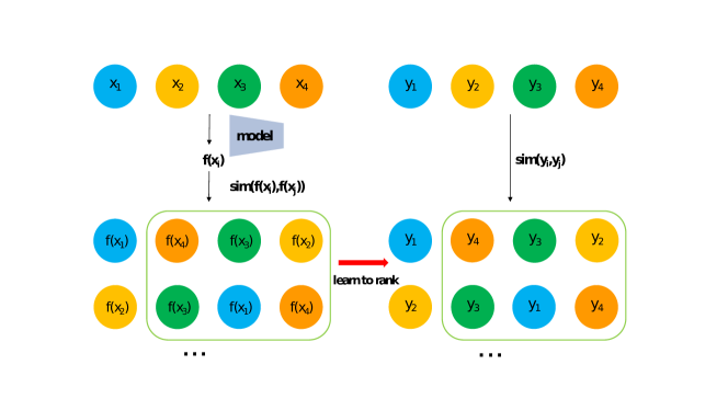
Figure 1: Assume that there are 4 samples $\{x_{1},x_{2},x_{3},x_{4}\}$ and the corresponding label $\{y_{1},y_{2},Y_{3},y_{4}\}$, for any query sample $x_{i}$ here I hope the corresponding feature similarity set $\{sim(f(x_{i}),f(x_{j})),j=1,2,3,4,j\neq i\}$ and label similarity set $\{sim(f(x_{i}),f(x_{j})),j=1,2,3\cdots n,j\neq\i\}$ keep the same sorting order.

How to keep the order relationship consistent? There are a variety of solutions in the field of learning to rank. Here, we uses the approximate NDCG indicator to achieve it. Select any sample $x_{i}$ from the sample set as the query sample, approximate NDCG indicator or A-NDCG loss can be formalized:

$$L(x)=\sum_{i}N_{i}^{-1}\sum_{j,j\neq i}^{n}(sim(y_{i},y_{j})/log_{2}(1+\pi(x_{i},x_{j}))$$ (5)

$$\pi(x_{i},x_{j}) = 1+\sum_{k,k\neq j}{\frac{exp(-\alpha sim_{ijk}))}{1+exp(-\alpha sim_{ijk})}}$$ (6)

$$sim_{ijk} = (sim(f(x_{i}),f(x_{j}))-sim(f(x_{i}),f(x_{k})))$$

Where $\alpha$ is the hyperparameter, and $N_{i}^{-1}$ is the normalization item, representing maximum value of $\sum\limits_{j,j\neq i}^{n}(sim(y_{i},y_{j})/log_{2}(1+\pi(x_{i},x_{j}))$: when the order of $\{sim(f(x_{i}),f(x_{j})),j=1,2,3\cdots n,j\neq i\}$ and $\{sim(y_{i},y_{j}),j=1,2,3\cdots n,j\neq i\}$ is same.

NDCG is not differentiable because of position item $j$. $\pi(x_{i},x_{j})$ in A-NDCG is the approximation of position item $j$ in NDCG indicate.

The advantages of approximate NDCG loss are: 1. The sample pair that needs to be selected for each calculation is $o(n^{2})$. Compared with some popular loss functions (Chen et al., 2020), the calculation complexity is lower. 2. It can naturally process any number of perspectives of the training data, which greatly relaxes the two perspectives of the popular contrastive learning algorithms (Chen et al., 2020; Grill et al., 2020). 3. Few constraints, only need to constrain the ordering relationship, no other conditions need to be constrained, which is conducive to learning robust representation. 4. Compared with the contrastive learning methods (Chen et al., 2020; Grill et al., 2020) and the learning to rank methods based on optimized average recall (Varamesh et al., 2020), the approximate NDCG loss is applicable to any situation where the label similarity set can be obtained. For training data with single label, multiple labels, discrete labels, and continuous labels, we can obtain the label similarity set, which also means that the approximate NDCG loss can handle a wide range of learning tasks and has a wide range of applications. 5. Thanks to the good ability to handle diversified labels, we can use label-level data augmentation methods on training data to enhance the performance of approximate NDCG loss continuously, so that the training data information can be fully utilized.

5 Experiment

In order to evaluate A-NDCG and verify its advantages, we conducts experiments under a variety of learning tasks. The experiments in this paper include learning representations under a variety of learning tasks: classification tasks, retrieval tasks, self-supervised tasks, multi-label classification, and regression tasks.

5.1 Classification Task

In the classification task, the learned representation should be able to make good use of linear classifiers such as softmax to solve classification tasks.

This paper will first use Cross-Entropy loss and its variant  (Liu et al., 2016) and the supervised contrast learning algorithm SupCon (Caron et al., 2020) as the comparison algorithm, and then use the classification accuracy rate of linear softmax classifier on the popular CIFAR-10 and CIFAR-100 dataset to estimate the approximate NDCG loss.

5.1.1 implementation details

For the approximate NDCG loss, this paper uses the standard residual network: resnet-50 as the encoder, and then imitates the standard practice  (Chen et al., 2020) to add a small projection network composed of two-layer MLP and Relu activation function behind the residual network. We use standard Adam optimizer (Kingma & Ba, 2014)

5.1.2 Experimental Results Analysis

The table 1 shows that the effect of A-NDCG on the CIFAR-10 and CIFAR-100 datasets exceeds the Cross-Entropy loss and some of its variants, such as Max-Margin (Liu et al., 2016). It is equivalent to the performance of SupCon (Khosla et al., 2020). Compared with Cross-Entropy loss and Max-Margin (Liu et al., 2016), they can use the relationship between sample pairs instead of just the relationship between a single sample and its label. They all relax the limitations of SimCLR (Chen et al., 2020) on the number of perspectives, and can make use of more comparative information between samples. But the training speed of Cross-Entropy loss is higher than A-NDCG and SupCon.

5.2 Retrieval Task

The image retrieval task is a standard evaluation task in the field of depth measurement. The representation learned under the retrieval task should be able to use linear learners such as knn to retrieve samples.

We will compare a variety of deep metric learning algorithms (Wang et al., 2019). We uses the standard data set: CUB-200-2011(Wah et al., 2011) to evaluate the retrieval performance of approximate NDCG loss.

The implementation details are consistent with the previous part.

5.2.1 Experimental Results Analysis

The table 2 shows that on the CUB-200-2011 dataset, the performance of A-NDCG exceeds many popular deep metric learning methods. In the specific implementation of this paper, the number of positive samples and negative samples involved in the calculation is the same as other methods. Compared with other methods, A-NDCG only needs to be constrain order relationship and no specific sample interval is specified, and its performance on the test data is more robust.

Table 1: Classification accuracy on CIFAR-10 and CIFAR-100 datasets

dataset	SimCLR	Cross-Entropy	Max-Margin(Liu et al., 2016)	SupCon(Caron et al., 2020)	A-NDCG
CIFAR10	93.6	95.0	92.4	96.0	95.3
CIFAR100	70.7	75.3	70.5	76.5	76.7

Table 2: Retrieval performance on CUB-200-2011 dataset, we use recall to estimate

Rank@K	1	2	4	8	16	32
Clustering64	48.2	61.4	71.8	81.9	-	-
ProxyNCA64	49.2	61.9	67.9	72.4	-	-
Smart Mining64	49.8	62.3	74.1	83.3	-	-
HTL512	57.1	68.8	78.7	86.5	92.5	95.5
ABIER512	57.5	68.7	78.3	86.2	91.9	95.5
MS-Loss512	57.5	70.3	80.0	88.0	93.2	96.2
A-NDCG512	58.3	70.7	80.5	88.5	93.8	96.9

5.3 Multi-label Learning

Multi-label learning is a traditional research direction, and there have been quite a lot of research results (Zhang & Zhou, 2007), where the representations obtained should be able to reduce the learning difficulty of other linear multi-label learning algorithms.

We uses Hamming loss and Jaccard score to evaluate the performance. The former uses Hamming distance to measure the difference between different multi-label labels, the lower the better, the latter measures the ratio of the intersection and union of two multi-label labels, the higher the better .

5.3.1 Dataset

We uses a variety of popular multi-label datasets . Core5k is an image dataset with 5000 images, Scene has more than 2000 images, Medical and Enron are two text data, Medical has 978 samples, and Enron has 1702 samples.

5.3.2 Evaluation Algorithm

MLKNN and BRKNN are two distance-based multi-label learning algorithms, we use them to evaluate A-NDCG.

5.3.3 Experimental Results Analysis

From the table 4, table 3, it can be clearly seen that as the number of iterations increases, the Hamming loss continues to decrease and the Jaccard score increase continually , A-NDCG loss is very effective in learning good representations on multi-labeled data. A-NDCG loss makes full use of the label information of the multi-labeled dataset, even for samples with very close multi-labeled labels. It can give specific optimization goals on how to distinguish them, so that the samples can distinguish samples with similar labels in the feature space, and ultimately reduce the learning difficulty of the linear multi-label learner.

Table 3: classification accuracy on muti-label datasets, we use MLKNN(Zhang & Zhou, 2007) to evaluate.

dataset	indicator	MLKNN	A-NDCG, epoch:10	20	30	40	50
Scene	Hamming Loss	0.102	0.095	0.088	0.090	0.088	0.093
	Jaccard Score	0.610	0.698	0.707	0.710	0.722	0.715
Corel5k	Hamming Loss	0.012	0.011	0.011	0.011	0.012	0.012
	Jaccard Score	0.094	0.1116	0.134	0.133	0.133	0.125
Medical	Hamming Loss	0.020	0.013	0.013	0.013	0.013	0.011
	Jaccard Score	0.512	0.726	0.74	0.74	0.74	0.739
Enron	Hamming Loss	0.062	0.05	0.05	0.05	0.05	0.056
	Jaccard Score	0.329	0.441	0.449	0.451	0.455	0.456

Table 4: classification accuracy, we use BRKNN (Eleftherios Spyromitros, 2008) to evaluate.

dataset	indicator	BRKNN	A-NDCG, epoch:10	20	30	40	50
Scene	Hamming Loss	0.109	0.095	0.095	0.090	0.089	0.091
	Jaccard Score	0.640	0.698	0.720	0.725	0.726	0.726
Corel5k	Hamming Loss	0.011	0.011	0.011	0.011	0.011	0.012
	Jaccard Score	0.069	0.123	0.140	0.145	0.149	0.142
Medical	Hamming Loss	0.020	0.014	0.013	0.013	0.014	0.013
	Jaccard Score	0.472	0.696	0.703	0.709	0.72	0.723
Enron	Hamming Loss	0.059	0.05	0.05	0.05	0.05	0.052
	Jaccard Score	0.324	0.44	0.46	0.46	0.46	0.472

5.4 Regression Task

The regression task is a widely used task. Time series forecasting, energy forecasting, financial market forecasting, etc. all have a great intersection with the regression task. The representation learned under the regression task should be able to reduce the learning difficulty of the linear regressor.

We use ridge regression and linear regression methods as evaluation algorithms. We use absolute loss MAE and mean square loss MSE as evaluation indicators to evaluate A-NDCG, both of which measure the error of the regression results, the lower the indicator, the better. We finds several regression data from the UCI data set, including housing price data, wine data and disease data parkinsons.

5.4.1 Experimental Analysis

In fact, the regression task is a challenge. It is not the same as the discriminative task. It has continuous labels, but A-NDCG can still learn a good representation in the regression datasets stably, reducing the learning difficulty of the regression method. There has been some work citehooshmand2019energy(Ye & Dai, 2018) combines the pre-training model with the prediction task. We thinks that A-NDCG can also be naturally applied to such tasks.

Table 5: result on regression datasets, we use ridge regression method to evaluate.

dataset	indicator	ridge	A-NDCG
parkinsons	MSE	91.4	77.61
	MAE	7.90	7.40
housing	MSE	18.61	-
	MAE	3.40	-
wine	MSE	0.62	0.59
	MAE	0.60	0.59

Table 6: result on regression datasets, we use linear regression methods to evaluate.

dataset	indicator	LR	A-NDCG
parkinsons	MSE	91.42	72.72
	MAE	7.433	7.044
housing	MSE	18.64	13.77
	MAE	3.398	2.95
wine	MSE	0.62	0.55
	MAE	0.60	0.58

5.5 Self-supervised Learning Task

Although there have been works that introduce the idea of learning to rank into the field of self-supervised learning (Varamesh et al., 2020), the optimization goal of this paper is different, (Varamesh et al., 2020) uses average recall as the optimization goal. Under self-supervised tasks, the representations learned using unsupervised data should be able to reduce the difficulty of supervised learning, such as improving the classification performance of linear learners.

We conduct experiments on the popular STL-10 dataset (Coates et al., 2011). In this paper, logistic regression and k-nearest neighbor classifier are used as methods for evaluating representations.

We will also use the data augmentation methods mixup(Zhang et al., 2017) and cutmix(Yun et al., 2019) to augment the training data at the label level to verify whether A-NDCG can make full use of the information in the unsupervised data.

Table 7: Classification accuracy on STL-10 dataset, we use logistic regression to evaluate.

method	epoch:0	4	8	12	16	20	24	28	32
SimCLR(train)	70.4	78.2	80.7	82.0	83.5	84.2	82.2	82.9	85.8
A-NDCG(train)	77.8	85.0	86.1	86.7	86.6	86.6	87.4	87.0	86.3
SimCLR(test)	44.0	49.8	51.8	52.3	51.6	52.7	52.7	52.6	51.7
A-NDCG(test)	44.0	49.5	51.9	52.3	51,8	52.1	52.8	50.9	52.4

Table 8: Classification accuracy on STL-10 dataset, we use knn to evaluate.

method	epoch:0	4	8	12	16	20	24	28	32
SimCLR(train)	59.2	62.4	62.9	64.5	64.5	65.0	65.0	65.9	66.1
A-NDCG(train)	62.2	66.1	66.6	67.5	68.3	67.4	67.8	67.9	68.9
SimCLR(test)	31.5	37.0	39.1	40.0	39.6	39.6	39.6	41.1	41.0
A-NDCG(test)	36.3	40.5	42.4	43.0	43.0	43.2	44.0	44.8	44.7

Table 9: Classifycation accuracy on mixed STL-10 dataset, we use logistic regression to evaluate

method	epoch:0	4	8	12	16	20	24	28	32
A-NDCG(train)	77.8	85.0	86.1	86.7	86.6	86.6	87.4	87.0	86.3
A-NDCG+mixup(train)	80.9	86.5	87.2	87.9	89.8	89.3	89.6	89.1	89.4
A-NDCG+cutmax(train)	88.4	86.4	87.1	87.5	87.6	87.3	87.8	87.7	88.3
A-NDCG(test)	44.0	49.5	51.9	52.3	51,8	52.1	52.8	50.9	52.4
A-NDCG+mixup(test)	44.9	52.0	52.7	53.1	53.8	54.3	53.8	54.8	55.7
A-NDCG+cutmax(test)	51.0	52.2	52.3	51.9	52.5	52.5	53.0	53.0	53.0

Table 10: Classifycation accuracy on mixed STL-10 dataset, we use knn to evaluate

method	epoch:0	4	8	12	16	20	24	28	32
A-NDCG(train)	62.2	66.1	66.6	67.5	68.3	67.4	67.8	67.9	68.9
A-NDCG+mixup(train)	64.8	68.1	68.9	69.7	68.8	70.5	70.3	71.3	70.8
A-NDCG+cutmax(train)	63.6	63.5	66.8	68.0	69.5	69.0	69.4	69.9	70.0
A-NDCG(test)	36.3	40.5	42.4	43.0	43.0	43.2	44.0	44.8	44.7
A-NDCG+mixup(test)	39.2	43.6	44.3	46.2	47.0	46.9	47.5	46.5	47.5
A-NDCG+cutmax(test)	37.7	42.1	42.6	44.4	44.6	45.4	46.3	45.9	45.8

5.5.1 implementation details

For the experiments on the STL-10 dataset, we keep consistent with the approach of (Varamesh et al., 2020). We use resnet-18 as the encoder, and then connects the projection network composed of two layers of mlp, the batch size is set to 32, the optimizer and the learning rate keep same wit SimCLR. The epoch is set to 36, and longer training time will bring better results.

5.5.2 Experimental Results Analysis

Table 7 and table 8 indicate that under the two evaluation algorithms, the performance of A-NDCG is better than SimCLR(Chen et al., 2020).Because there is no limit to the number of perspectives of a single data. According to the perspective of contrastive learning, A-NDCG is comparing the difference between the sample feature similarity set that is not sorted according to the real ranking relationship and the sample feature similarity set that is sorted according to the real ranking relationship, not comparing the difference between positive sample pair similarity and negative sample pair similarity, it surpasses the conceptual constraints of positive sample and negative sample, and has broader meaning and applicability. The table 9 and the table 10 show that: A-NDCG can make full use of the label-level data augmentation methods to transform the training data in order to make full use of the information in the unsupervised data, despite the manual designed data augmentation method will bring a lot of noise and errors, but because the constraints of A-NDCG are very loose and the influence of noise is reduced, it can be seen that the improvement effect of A-NDCG is still very obvious. Making full use of the various information of unsupervised training data, which is obviously necessary for unsupervised learning.

6 Conclution

In this paper, the representation learning problem under multiple tasks is modeled as a ranking problem, and taking the ranking problem as a unified perspective, the representation learning problem under different tasks is solved by optimizing the approximate NDCG loss. And divided into learning tasks, we organized a large number of experiments, through the classification, retrieval, multi-label learning, regression, self-supervised learning experiments proved the superiority of the approximate NDCG loss. Further, under the self-supervised learning task, the training data is transformed by data augmentation method to improve the performance of the approximate NDCG loss, which proves that the approximate NDCG loss can make full use of the unsupervised data information.

References

- Baeza-Yates et al. (1999) Baeza-Yates, R., Ribeiro-Neto, B., et al. Modern information retrieval, volume 463. ACM press New York, 1999.
- Bengio et al. (2013) Bengio, Y., Courville, A., and Vincent, P. Representation learning: A review and new perspectives. IEEE transactions on pattern analysis and machine intelligence, 35(8):1798–1828, 2013.
- Brown et al. (2020) Brown, A., Xie, W., Kalogeiton, V., and Zisserman, A. Smooth-ap: Smoothing the path towards large-scale image retrieval. In European Conference on Computer Vision, pp. 677–694. Springer, 2020.
- Cakir et al. (2019) Cakir, F., He, K., Xia, X., Kulis, B., and Sclaroff, S. Deep metric learning to rank. In Proceedings of the IEEE Conference on Computer Vision and Pattern Recognition, pp. 1861–1870, 2019.
- Caron et al. (2018) Caron, M., Bojanowski, P., Joulin, A., and Douze, M. Deep clustering for unsupervised learning of visual features. In Proceedings of the European Conference on Computer Vision (ECCV), pp. 132–149, 2018.
- Caron et al. (2020) Caron, M., Misra, I., Mairal, J., Goyal, P., Bojanowski, P., and Joulin, A. Unsupervised learning of visual features by contrasting cluster assignments. arXiv preprint arXiv:2006.09882, 2020.
- Chen et al. (2020) Chen, T., Kornblith, S., Norouzi, M., and Hinton, G. A simple framework for contrastive learning of visual representations. arXiv preprint arXiv:2002.05709, 2020.
- Chen & He (2020) Chen, X. and He, K. Exploring simple siamese representation learning. arXiv preprint arXiv:2011.10566, 2020.
- Chen et al. (2016) Chen, X., Duan, Y., Houthooft, R., Schulman, J., Sutskever, I., and Abbeel, P. Infogan: Interpretable representation learning by information maximizing generative adversarial nets. Advances in neural information processing systems, 29:2172–2180, 2016.
- Coates et al. (2011) Coates, A., Ng, A., and Lee, H. An analysis of single-layer networks in unsupervised feature learning. In Proceedings of the fourteenth international conference on artificial intelligence and statistics, pp. 215–223. JMLR Workshop and Conference Proceedings, 2011.
- Devlin et al. (2018) Devlin, J., Chang, M.-W., Lee, K., and Toutanova, K. Bert: Pre-training of deep bidirectional transformers for language understanding. arXiv preprint arXiv:1810.04805, 2018.
- Donahue & Simonyan (2019) Donahue, J. and Simonyan, K. Large scale adversarial representation learning. In Advances in Neural Information Processing Systems, pp. 10542–10552, 2019.
- Donahue et al. (2016) Donahue, J., Krähenbühl, P., and Darrell, T. Adversarial feature learning. arXiv preprint arXiv:1605.09782, 2016.
- Dupont (2018) Dupont, E. Learning disentangled joint continuous and discrete representations. In Advances in Neural Information Processing Systems, pp. 710–720, 2018.
- Eleftherios Spyromitros (2008) Eleftherios Spyromitros, Grigorios Tsoumakas, I. V. An empirical study of lazy multilabel classification algorithms. In Proc. 5th Hellenic Conference on Artificial Intelligence (SETN 2008), 2008.
- Grill et al. (2020) Grill, J.-B., Strub, F., Altché, F., Tallec, C., Richemond, P. H., Buchatskaya, E., Doersch, C., Pires, B. A., Guo, Z. D., Azar, M. G., et al. Bootstrap your own latent: A new approach to self-supervised learning. arXiv preprint arXiv:2006.07733, 2020.
- Hadsell et al. (2006) Hadsell, R., Chopra, S., and LeCun, Y. Dimensionality reduction by learning an invariant mapping. In 2006 IEEE Computer Society Conference on Computer Vision and Pattern Recognition (CVPR’06), volume 2, pp. 1735–1742. IEEE, 2006.
- Hjelm et al. (2018) Hjelm, R. D., Fedorov, A., Lavoie-Marchildon, S., Grewal, K., Bachman, P., Trischler, A., and Bengio, Y. Learning deep representations by mutual information estimation and maximization. arXiv preprint arXiv:1808.06670, 2018.
- Järvelin & Kekäläinen (2002) Järvelin, K. and Kekäläinen, J. Cumulated gain-based evaluation of ir techniques. ACM Transactions on Information Systems (TOIS), 20(4):422–446, 2002.
- Khosla et al. (2020) Khosla, P., Teterwak, P., Wang, C., Sarna, A., Tian, Y., Isola, P., Maschinot, A., Liu, C., and Krishnan, D. Supervised contrastive learning. arXiv preprint arXiv:2004.11362, 2020.
- Kim & Mnih (2018) Kim, H. and Mnih, A. Disentangling by factorising. arXiv preprint arXiv:1802.05983, 2018.
- Kingma & Ba (2014) Kingma, D. P. and Ba, J. Adam: A method for stochastic optimization. arXiv preprint arXiv:1412.6980, 2014.
- Kingma & Welling (2013) Kingma, D. P. and Welling, M. Auto-encoding variational bayes. arXiv preprint arXiv:1312.6114, 2013.
- Liu et al. (2016) Liu, W., Wen, Y., Yu, Z., and Yang, M. Large-margin softmax loss for convolutional neural networks. In ICML, volume 2, pp. 7, 2016.
- Oord et al. (2017) Oord, A. v. d., Vinyals, O., and Kavukcuoglu, K. Neural discrete representation learning. arXiv preprint arXiv:1711.00937, 2017.
- Oord et al. (2018) Oord, A. v. d., Li, Y., and Vinyals, O. Representation learning with contrastive predictive coding. arXiv preprint arXiv:1807.03748, 2018.
- Qin et al. (2010) Qin, T., Liu, T.-Y., and Li, H. A general approximation framework for direct optimization of information retrieval measures. Information retrieval, 13(4):375–397, 2010.
- Shen et al. (2020) Shen, Z., Liu, Z., Liu, Z., Savvides, M., and Darrell, T. Rethinking image mixture for unsupervised visual representation learning. arXiv preprint arXiv:2003.05438, 2020.
- Sohn (2016) Sohn, K. Improved deep metric learning with multi-class n-pair loss objective. Advances in neural information processing systems, 29:1857–1865, 2016.
- Sun et al. (2020) Sun, Y., Cheng, C., Zhang, Y., Zhang, C., Zheng, L., Wang, Z., and Wei, Y. Circle loss: A unified perspective of pair similarity optimization. In Proceedings of the IEEE/CVF Conference on Computer Vision and Pattern Recognition, pp. 6398–6407, 2020.
- Tian et al. (2020) Tian, Y., Sun, C., Poole, B., Krishnan, D., Schmid, C., and Isola, P. What makes for good views for contrastive learning. arXiv preprint arXiv:2005.10243, 2020.
- Tschannen et al. (2019) Tschannen, M., Djolonga, J., Rubenstein, P. K., Gelly, S., and Lucic, M. On mutual information maximization for representation learning. arXiv preprint arXiv:1907.13625, 2019.
- Varamesh et al. (2020) Varamesh, A., Diba, A., Tuytelaars, T., and Van Gool, L. Self-supervised ranking for representation learning. arXiv preprint arXiv:2010.07258, 2020.
- Wah et al. (2011) Wah, C., Branson, S., Welinder, P., Perona, P., and Belongie, S. The Caltech-UCSD Birds-200-2011 Dataset. Technical Report CNS-TR-2011-001, California Institute of Technology, 2011.
- Wang et al. (2019) Wang, X., Han, X., Huang, W., Dong, D., and Scott, M. R. Multi-similarity loss with general pair weighting for deep metric learning. In Proceedings of the IEEE/CVF Conference on Computer Vision and Pattern Recognition, pp. 5022–5030, 2019.
- Wen et al. (2016) Wen, Y., Zhang, K., Li, Z., and Qiao, Y. A discriminative feature learning approach for deep face recognition. In European conference on computer vision, pp. 499–515. Springer, 2016.
- Xia et al. (2008) Xia, F., Liu, T.-Y., Wang, J., Zhang, W., and Li, H. Listwise approach to learning to rank: theory and algorithm. In Proceedings of the 25th international conference on Machine learning, pp. 1192–1199, 2008.
- Xu et al. (2008) Xu, J., Liu, T.-Y., Lu, M., Li, H., and Ma, W.-Y. Directly optimizing evaluation measures in learning to rank. In Proceedings of the 31st annual international ACM SIGIR conference on Research and development in information retrieval, pp. 107–114, 2008.
- Ye & Dai (2018) Ye, R. and Dai, Q. A novel transfer learning framework for time series forecasting. Knowledge-Based Systems, 156:74–99, 2018.
- Yun et al. (2019) Yun, S., Han, D., Oh, S. J., Chun, S., Choe, J., and Yoo, Y. Cutmix: Regularization strategy to train strong classifiers with localizable features. In Proceedings of the IEEE/CVF International Conference on Computer Vision, pp. 6023–6032, 2019.
- Zhang et al. (2017) Zhang, H., Cisse, M., Dauphin, Y. N., and Lopez-Paz, D. mixup: Beyond empirical risk minimization. arXiv preprint arXiv:1710.09412, 2017.
- Zhang & Zhou (2007) Zhang, M.-L. and Zhou, Z.-H. Ml-knn: A lazy learning approach to multi-label learning. Pattern recognition, 40(7):2038–2048, 2007.