ACSNet: Action-Context Separation Network for Weakly Supervised
Temporal Action Localization

Abstract

The object of Weakly-supervised Temporal Action Localization (WS-TAL) is to localize all action instances in an untrimmed video with only video-level supervision. Due to the lack of frame-level annotations during training, current WS-TAL methods rely on attention mechanisms to localize the foreground snippets or frames that contribute to the video-level classification task. This strategy frequently confuse context with the actual action, in the localization result. Separating action and context is a core problem for precise WS-TAL, but it is very challenging and has been largely ignored in the literature. In this paper, we introduce an Action-Context Separation Network (ACSNet) that explicitly takes into account context for accurate action localization. It consists of two branches (i.e., the Foreground-Background branch and the Action-Context branch). The Foreground-Background branch first distinguishes foreground from background within the entire video while the Action-Context branch further separates the foreground as action and context. We associate video snippets with two latent components (i.e., a positive component and a negative component), and their different combinations can effectively characterize foreground, action and context. Furthermore, we introduce extended labels with auxiliary context categories to facilitate the learning of action-context separation. Experiments on THUMOS14 and ActivityNet v1.2/v1.3 datasets demonstrate the ACSNet outperforms existing state-of-the-art WS-TAL methods by a large margin.

1 Introduction

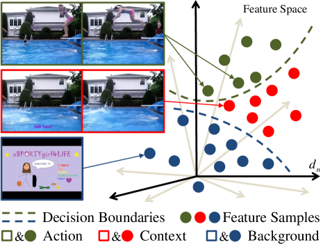
Figure 1: The illustration of action, context and background in terms of frames and points in feature space. The green dashed line is the desired boundary for the localization task. However, based on the given video-level categorical labels, the blue dashed line is learned, due to the high co-occurrence and visual similarity of action and context. Existing methods frequently identify both red and green dots as actions. The main challenge in WS-TAL is how to isolate context from action instances with merely video-level categorical labels

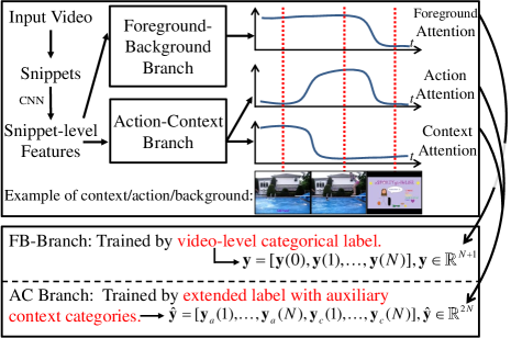
Figure 2: An overview of our main idea, i.e., using extended label with auxiliary context categories to guide the training of action/context attentions. Unfortunately, such an idea is nontrivial to implement due to “lack of explicit action-context constraint” and “lack of explicit supervision”.

Temporal Action Localization (TAL) aims to localize temporal starts and ends of specific action categories in a video. It serves as a fundamental tool for several practical applications such as action retrieval, intelligent surveillance and video summarization (Lee, Ghosh, and Grauman 2012; Vishwakarma and Agrawal 2013; Asadiaghbolaghi et al. 2017; Kang and Wildes 2016; Yao, Lei, and Zhong 2019). Although fully supervised TAL methods have recently achieved remarkable progress (Buch et al. 2017; Xu, Das, and Saenko 2017; Gao et al. 2017; Xu, Das, and Saenko 2017; Chao et al. 2018; Lin et al. 2018, 2019; Zeng et al. 2019), manually annotating the precise temporal boundaries of action instances in untrimmed videos is time-consuming and challenging. This limitation motivates the weakly supervised setting where only video-level categorical labels are provided for model training. Compared with temporal boundary annotations, video-level categorical labels are easier to collect, and they help avoid the localization bias introduced by human annotators.

Existing weakly-supervised temporal action localization (WS-TAL) methods (Wang et al. 2017; Nguyen et al. 2018; Paul, Roy, and Roy-Chowdhury 2018; Nguyen, Ramanan, and Fowlkes 2019) leverage attention mechanisms to categorize snippets or sampled frames into foreground and background based on their contribution to the video-level classification task, i.e., to find the blue dashed line in Figure 1. Then temporal action localization is reformulated as selecting consecutive foreground snippets belonging to each category. However, the foreground localized through video-level categorization involves not only the actual action instance but also its surrounding context. As illustrated in Figure 1, context is snippets or frames that frequently co-occur with the action instances of a specific category but should not be included in their localization. Different from background, which is class-agnostic, context provides strong evidence for action classification and thus can be easily confused with the action instances. We believe separating the action instances and their context is a core problem in WS-TAL, and it is very challenging due to the co-occurrence nature.

The goal of this paper is to address the action-context separation (ACS) problem in the weakly-supervised setting so as to achieve more precise action localization. We first introduce auxiliary context categories for each action class during training. As shown in Figure 2, each video-level category is divided into two sub-categories, respectively corresponding to the actual action and its context. Prior methods exploit foreground attention to achieve foreground-background separation. However, this simple idea is not applicable to action-context separation due to two difficult issues. (1) Lack of explicit action-context constraints: The sum-to-one constraint  (Nguyen, Ramanan, and Fowlkes 2019) of the foreground and background attention scores does not apply to action-context separation. (2) Lack of explicit supervision: Both action and context can contribute to action classification, so the only available video-level categorical labels cannot provide direct supervision for them.

To address these two difficult issues, we introduce the Action-Context Separation Network (ACSNet). As illustrated in Figure 3, it consists of two branches, i.e., the Foreground-Background branch (FB branch) and the Action-Context branch (AC branch). The FB branch divides an untrimmed video into foreground and background based on whether a snippet supports the video-level classification. This is achieved via snippet-level categorical predictions (SCPs) and snippet-level attention predictions (SAPs), e.g., foreground attention in Figure 2. Subsequently, the AC branch further divides the obtained foreground into action and context by associating each video snippet with two latent components, i.e., a positive component and a negative component. Different combinations of these two components respectively characterize the foreground, action and context. This enables effective action-context separation with only video-level supervision. Finally, the output of AC branch facilitates the TAL by providing (1) temporal action proposals with more accurate boundaries and (2) more reliable proposal confidence scores.

The contribution of this paper is summarized below.

1. Prior WS-TAL approaches take it for granted that the foreground localized via the classification attention is equivalent to the actual action instance, and thus they unavoidably include the co-occurring context in the localization result. We address this challenge via a novel action-context separation network (ACSNet), which not only distinguishes foreground from background but also separates action and context within the foreground to achieve more precise action localization.

2. The proposed ACSNet features a novel Action-Context branch. It can individually characterize foreground, action and context using different combinations of two latent components, i.e., the positive component and the negative component.

3. We propose novel extended labels with auxiliary context categories. By explicitly decoupling the actual action and its context, this new representation facilitates effective learning of action-context separation.

4. Extensive experimental results indicate the proposed ACSNet can effectively perform action-context separation. It significantly outperforms state-of-the-art methods on three benchmarks, and it is even comparable to recent fully-supervised methods.

2 Related Work of WS-TAL

Different from action recognition which is essentially a classification task (Feichtenhofer, Pinz, and Zisserman 2016; Simonyan and Zisserman 2014; Wang et al. 2016; Ji et al. 2013; Sun et al. 2015b; Tran et al. 2015; Feichtenhofer et al. 2019), TAL requires finer-grained predictions with temporal boundaries of the target action instances. WS-TAL methods address it without temporal annotations, which is first introduced in (Sun et al. 2015a). To distinguish action instances from background, the attention mechanism is widely adopted for foreground-background separation. UntrimmedNet (Wang et al. 2017) formulates the attention mechanism as a soft selection module to localize target action, and the final localization is achieved by thresholding the snippets’ action scores. STPN (Nguyen et al. 2018) proposes a sparsity loss based on the soft selection module of UntrimmedNet, which can facilitate the selection of action instances. Nguyen et al. (Nguyen, Ramanan, and Fowlkes 2019) characterize background by an additional background loss and introduce other losses to guide the attention. For better evaluation of temporal action proposals, W-TALC (Paul, Roy, and Roy-Chowdhury 2018) proposes a co-activity loss to enforce the feature similarity among localized instances. AutoLoc (Shou et al. 2018) uses an “outer-inner-contrastive loss” to predict and regress temporal boundaries. Liu et al. (Liu, Jiang, and Wang 2019) exploit a multi-branch neural network to discover distinctive action parts and fuse them to ensure completeness. CleanNet (Liu et al. 2019b) designs a “contrast score” by leveraging temporal contrast in SCPs to achieve end-to-end training of localization.

However, driven by the video-level classification labels, the existing attention mechanism is merely able to capture the difference between foreground and background for classification, instead of action and non-action for localization. The proposed ACSNet manages to distinguish action instances from their surrounding context, and we extend labels by introducing auxiliary context categories to make the framework trainable.

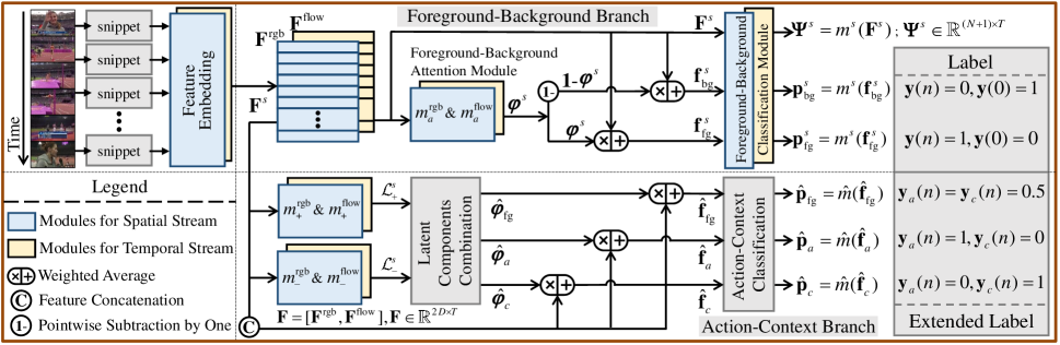
Figure 3: The framework of the proposed ACSNet, which has two branches, i.e., Foreground-Background branch and Action-Context branch. The input video is first processed by the feature embedding to get features from both spatial and temporal streams. The FB branch focuses on foreground-background separation while the AC branch focuses on action-context separation. Video-level labels are extended to facilitate the action-context separation.

3 Action-Context Separation Network

In this section, we introduce the extended video-level labels with auxiliary context categories (Section 3.1) and the proposed Action-Context Separation Network (ACSNet). As illustrated in Figure 3, the ACSNet consists of two branches, i.e., Foreground-Background branch (FB branch) and Action-Context branch (AC branch). After feature extraction from the given video (Section 3.2), FB branch distinguishes the foreground from background (Section 3.2). The obtained foreground contains both action and context. Subsequently, AC branch localizes the actual temporal action instances by performing action-context separation within the foreground (Section 3.3). To guide the training of ACS, additional losses are introduced (Section 3.4).

3.1 Extending Video-Level Labels

Suppose we are given a video $V$ with a video-level categorical label $\mathbf{y}=[\mathbf{y}(0),\mathbf{y}(1),\dots,\mathbf{y}(N)]$, where $\mathbf{y}(n)=1$ if $V$ contains the $n$-th action category. $N$ is the total number of action categories, $\mathbf{y}(0)$ represents the background category. To guide the division of foreground into action and context, we extend $\mathbf{y}$ with auxiliary context categories as

$$\mathbf{\widehat{y}}=[\mathbf{y}_{a}(1),\dots,\mathbf{y}_{a}(N),~{}\mathbf{y}_{c}(1),\dots,\mathbf{y}_{c}(N)],~{}\mathbf{\widehat{y}}\in\mathbb{R}^{2N},$$ (1)

where $\mathbf{y}_{a}(n)$ and $\mathbf{y}_{c}(n)$ denote the $n$-th action category and its corresponding context, respectively. As shown in Figure 3, $\mathbf{y}\in\mathbb{R}^{N+1}$ is used in FB branch and $\mathbf{\widehat{y}}\in\mathbb{R}^{2N}$ is used in AC branch.

3.2 Baseline Modules

This section introduces the baseline modules used in ACSNet, including feature extraction and FB branch based on the attention mechanism. While they are not our main contribution, we introduce them for completeness. Similar modules have been explored and adopted by existing methods (Nguyen et al. 2018; Paul, Roy, and Roy-Chowdhury 2018; Nguyen, Ramanan, and Fowlkes 2019; Lee, Uh, and Byun 2020).

Feature Extraction

The input of the feature extraction module is the given video $V=\{s_{t}\}_{t=1}^{T}$, which is divided into $T$ non-overlapping snippets. The outputs are the corresponding features of each snippet. For each snippet $s_{t}$, the corresponding $D$-dimensional features are extracted from two streams, i.e., the spatial stream (RGB) and the temporal stream (optical flow), denoted as $\mathbf{F}^{\textrm{rgb}}(t)\in\mathbb{R}^{D}$ and $\mathbf{F}^{\textrm{flow}}(t)\in\mathbb{R}^{D}$, respectively. Afterwards, the video $V$ is represented as $\mathbf{F}^{\textrm{rgb}}\in\mathbb{R}^{D\times T}$ and $\mathbf{F}^{\textrm{flow}}\in\mathbb{R}^{D\times T}$.

For notational simplicity, we use superscript “$s$” to indicate the notations used in both streams in the rest of the paper. The notations of the spatial/temporal stream can be obtained by substituting the superscript “$s$” with “rgb/flow”. For example, $\mathbf{F}^{s}$ can represent either $\mathbf{F}^{\textrm{rgb}}$ or $\mathbf{F}^{\textrm{flow}}$.

Foreground-Background Branch

The goal of the FB branch is to divide the entire video into two parts, i.e., foreground and background, which can be trained by the video-level categorical label $\mathbf{y}=[\mathbf{y}(0),\mathbf{y}(1),\dots,\mathbf{y}(N)]$.

The inputs of FB branch are the features $\mathbf{F}^{s}\!\in\!\mathbb{R}^{D\times T}$, and the outputs are the snippet-level attention predictions (SAPs, ${\boldsymbol{\varphi}}\!\in\!\mathbb{R}^{1\times T}$) and the snippet-level classification predictions (SCPs, ${\boldsymbol{\Psi}}\!\in\!\mathbb{R}^{(N\!+\!1)\times T}$). Accordingly, FB branch consists of two sub-modules, i.e., attention module ($m_{a}^{s}$) and Foreground-Background classification module ($m^{s}$). The SAPs and SCPs of each stream are obtained by

$$\boldsymbol{\varphi}^{\textrm{s}}=m_{a}^{s}(\mathbf{F}^{s}),~{}~{}\boldsymbol{\varphi}^{\textrm{s}}\in\mathbb{R}^{1\times T},$$ (2)

$$\boldsymbol{\Psi}^{{s}}=m^{s}(\mathbf{F}^{s}),~{}~{}\boldsymbol{\Psi}^{{s}}\in\mathbb{R}^{(N+1)\times T}.$$ (3)

Subsequently, the outputs of two streams are weighted to get the final SAPs and SCPs as

$${\boldsymbol{\varphi}}=\alpha\boldsymbol{\varphi}^{\textrm{rgb}}+(1-\alpha)\boldsymbol{\varphi}^{\textrm{flow}},$$ (4)

$${\boldsymbol{\Psi}}=\alpha\boldsymbol{\Psi}^{\textrm{rgb}}+(1-\alpha)\boldsymbol{\Psi}^{\textrm{flow}},$$ (5)

where $\alpha=0.5$ by default in our experiments. We implement $m_{a}^{s}$ with a fully-connected (FC) layer followed by a sigmoid activation function. And $m^{s}$ is implemented by an FC layer.

To train $m_{a}^{s}$ and $m^{s}$ with only video-level label, video-level prediction is needed. Therefore, we calculate the video-level foreground feature as

$$\mathbf{f}_{\textrm{fg}}^{s}=\frac{1}{T}\sum_{t=1}^{T}\boldsymbol{\varphi}^{{s}}(t)\mathbf{F}^{s}(t),~{}\mathbf{f}_{\textrm{fg}}^{s}\in\mathbb{R}^{D}.$$ (6)

Similarly, the video-level background feature is obtained by

$$\mathbf{f}_{\textrm{bg}}^{s}=\frac{1}{T}\sum_{t=1}^{T}(1-\boldsymbol{\varphi}^{{s}}(t))\mathbf{F}^{s}(t),~{}\mathbf{f}_{bg}^{s}\in\mathbb{R}^{D}.$$ (7)

After obtaining $\mathbf{f}_{\textrm{fg}}^{s}$ and $\mathbf{f}_{\textrm{bg}}^{s}$, we feed them into $m^{s}$ to obtain the video-level prediction, i.e., the foreground prediction ($\mathbf{p}_{\textrm{fg}}^{s}\in\mathbb{R}^{N+1}$) and background prediction ($\mathbf{p}_{\textrm{bg}}^{s}\in\mathbb{R}^{N+1}$), defined as

$$\mathbf{p}_{\textrm{fg}}^{s}=m^{s}(\mathbf{f}_{\textrm{fg}}^{s}),~{}\mathbf{p}_{\textrm{bg}}^{s}=m^{s}(\mathbf{f}_{\textrm{bg}}^{s}).$$ (8)

Given video-level predictions in Eq.(8), the FB branch can be trained via regular cross-entropy loss. For $\mathbf{p}_{\textrm{fg}}^{s}$, its label is $\mathbf{{y}}$, where $\mathbf{y}(n)=1$ if $V$ contains the $n$-th action category, as shown in Figure 3. While for $\mathbf{p}_{\textrm{bg}}^{s}$, assuming that all videos contain background snippets, its label is always $\mathbf{y}(0)=1$ and $\mathbf{y}(n)=0,~{}n=1,2,...N$.

3.3 Action-Context Branch

The attention mechanism trained by $\mathbf{y}$ will be distracted by context because both action and context can support video-level classification. To avoid such distraction, after distinguishing the foreground from background, we further separate action and context within the foreground to locate the actual action instances in this section.

The inputs of the AC branch are features from two streams ($\mathbf{F}^{s}$ obtained in Section 3.2) and SAPs (${\boldsymbol{\varphi}}$ obtained in Section 3.2). The AC branch consists of three sub-modules, i.e., latent components generation, latent components combination, and action-context separation.

Latent Components Generation.

We introduce the concept of positive component ($\mathcal{L}^{s}_{+}\in\mathbb{R}^{1\times T}$) and negative component ($\mathcal{L}^{s}_{-}\in\mathbb{R}^{1\times T}$) to characterize foreground, action and context. Assuming the foreground is represented by two latent components, we define the one corresponding to the actual action as positive component, while the other one as negative component. They are obtained similarly as the SAPs in Eq.(2), by feeding features into positive module ($m_{+}^{s}$) and negative module ($m_{-}^{s}$)

$$\mathcal{L}^{s}_{+}=m_{+}^{s}(\mathbf{F}^{s}),~{}\mathcal{L}^{s}_{-}=m_{-}^{s}(\mathbf{F}^{s}).$$ (9)

$m_{+}^{s}$ and $m_{-}^{s}$ share the same architecture (parameters are not shared), with two temporal convolution (Conv1d) layers followed by a ReLU and a sigmoid activation function for the first and the second layer, respectively.

Latent Components Combination.

Given $\mathcal{L}^{s}_{+}$ and $\mathcal{L}^{s}_{-}$, we use the combination of them to construct the snippet-level foreground attention ($\widehat{\boldsymbol{\varphi}}_{\textrm{fg}}\in\mathbb{R}^{1\times T}$), action attention ($\widehat{\boldsymbol{\varphi}}_{\textrm{a}}\in\mathbb{R}^{1\times T}$), and context attention ($\widehat{\boldsymbol{\varphi}}_{\textrm{c}}\in\mathbb{R}^{1\times T}$). Specifically, for each stream, we have

$$\widehat{\boldsymbol{\varphi}}_{\textrm{fg}}^{s}=\sigma(\mathcal{L}^{s}_{+}+\mathcal{L}^{s}_{-}),$$ (10)

$$\widehat{\boldsymbol{\varphi}}_{\textrm{a}}^{s}=\sigma(\mathcal{L}^{s}_{+}),$$ (11)

$$\widehat{\boldsymbol{\varphi}}_{\textrm{c}}^{s}=\sigma(\mathcal{L}^{s}_{-}-\mathcal{L}^{s}_{+}),$$ (12)

where $\sigma(\cdot)$ denotes the sigmoid function. Subsequently, the outputs from two streams are fused by weighted average similar to Eq.(4),

$$\widehat{\boldsymbol{\varphi}}_{{z}}=\alpha\widehat{\boldsymbol{\varphi}}_{{z}}^{\textrm{rgb}}+(1-\alpha)\widehat{\boldsymbol{\varphi}}_{{z}}^{\textrm{flow}},~{}\widehat{\boldsymbol{\varphi}}_{{z}}~{}z\in\{\textrm{fg},a,c\},$$ (13)

where $\widehat{\boldsymbol{\varphi}}_{{z}}\in\mathbb{R}^{1\times T}$. For notational simplicity, we use subscript “$z$” to denote either “fg”, “$a$” or“$c$” if necessary. By substituting the subscript “$z$” with “fg/$a$/$c$”, $\widehat{\boldsymbol{\varphi}}_{\textrm{fg}}$/$\widehat{\boldsymbol{\varphi}}_{\textrm{a}}$/$\widehat{\boldsymbol{\varphi}}_{\textrm{c}}$ are obtained following Eq.(13).

Instead of directly imposing simple constrains like foreground and background following (Nguyen, Ramanan, and Fowlkes 2019), i.e., $\widehat{\boldsymbol{\varphi}}_{\textrm{c}}^{s}=1-\widehat{\boldsymbol{\varphi}}_{\textrm{a}}^{s}$, we adopt the combinations of $\mathcal{L}^{s}_{+}$ and $\mathcal{L}^{s}_{-}$ to characterize $\widehat{\boldsymbol{\varphi}}_{\textrm{a}}^{s}$ and $\widehat{\boldsymbol{\varphi}}_{\textrm{c}}^{s}$ individually. We compared different approaches to obtain $\widehat{\boldsymbol{\varphi}}_{\textrm{c}}^{s}$ in supplementary material.

Action-Context Separation.

After obtaining $\widehat{\boldsymbol{\varphi}}_{\textrm{fg}}$, $\widehat{\boldsymbol{\varphi}}_{\textrm{a}}$ and $\widehat{\boldsymbol{\varphi}}_{\textrm{c}}$, we can start the action-context separation by leveraging label with auxiliary context categories (i.e., $\mathbf{\widehat{y}}\in\mathbb{R}^{2N}$ introduced in Section 3.1). First of all, we select all temporal indices corresponding to foreground snippets as

$$\mathbb{I}=\{t~{}|~{}{\boldsymbol{\varphi}}(t)>0.5\},~{}|\mathbb{I}|=T^{\prime},$$ (14)

where $|\cdot|$ denotes the cardinality (number of elements). Subsequently, the video-level feature representations of foreground, action and context are obtained as

$$\widehat{\mathbf{f}}_{z}=\frac{1}{T^{\prime}}\sum_{t\in\mathbb{I}}\widehat{\boldsymbol{\varphi}}_{{z}}(t)\mathbf{F}(t),~{}z\in\{\textrm{fg},a,c\},$$ (15)

where $\widehat{\mathbf{f}}_{z}\in\mathbb{R}^{2D\times 1}$ and $\mathbf{F}(t)=\langle\mathbf{F}^{\textrm{rgb}}(t),\mathbf{F}^{\textrm{flow}}(t)\rangle~{}(\mathbf{F}(t)\!\in\!\mathbb{R}^{2D\times 1})$ is the concatenated feature from both streams and $\langle\cdot\rangle$ means concatenation. By substituting the subscript “$z$” with “fg/$a$/$c$”, $\widehat{\mathbf{f}}_{\textrm{fg}}$, $\widehat{\mathbf{f}}_{a}$ and $\widehat{\mathbf{f}}_{c}$ are calculated following Eq.(15). Afterwards, they are fed into the action-context classification module $\widehat{m}$ to get the video-level action-context prediction as

$$\widehat{\mathbf{p}}_{z}=\widehat{m}(\widehat{\mathbf{f}}_{z}),\widehat{\mathbf{p}}_{z}\in\mathbb{R}^{2N},~{}z\in\{\textrm{fg},a,c\}.$$ (16)

Different from the video-level prediction from FB branch (i.e., $\mathbf{p}_{\textrm{fg}}^{s}\in\mathbb{R}^{N+1}$ in Eq.(8)), $\widehat{\mathbf{p}}_{z}\in\mathbb{R}^{2N}$ provides predictions on both action and context categories. Specifically, if the video contains the $n$-th category, the label for $\widehat{\mathbf{p}}_{\textrm{fg}}$ is $\mathbf{\widehat{y}}=[\mathbf{y}_{a}(1),\dots,\mathbf{y}_{a}(N),~{}\mathbf{y}_{c}(1),\dots,\mathbf{y}_{c}(N)]$, where $\mathbf{y}_{a}(n)=\mathbf{y}_{c}(n)=0.5$. While for $\widehat{\mathbf{p}}_{a}$ and $\widehat{\mathbf{p}}_{c}$, the labels are ($\mathbf{y}_{a}(n)=1,\mathbf{y}_{c}(n)=0$) and ($\mathbf{y}_{a}(n)=0,\mathbf{y}_{c}(n)=1$), respectively, as shown in Figure 3. After obtaining $\widehat{\mathbf{p}}_{z}$ and the corresponding labels, the AC branch is also trained via regular cross-entropy loss.

Applying $\widehat{m}$ to each snippet, the snippet-level action-context predictions are obtained as

$${\boldsymbol{\Psi}}^{\prime}=\widehat{m}(\mathbf{F}),~{}{\boldsymbol{\Psi}}^{\prime}\in\mathbb{R}^{2N\times T},$$ (17)

where $\mathbf{F}\in\mathbb{R}^{2D\times T}$ is the concatenated feature. ${\boldsymbol{\Psi}}^{\prime}$ is leveraged to promote the action and suppress the context, by defining an “action-context offset ($\widehat{\boldsymbol{\Psi}}\!\in\!\mathbb{R}^{N\times T}$)” as

$$\widehat{\boldsymbol{\Psi}}(n,t)\!=\!\begin{cases}{\boldsymbol{\Psi}}^{\prime}(n,t)\!-\!{\boldsymbol{\Psi}}^{\prime}(2n,t)~{}~{}~{}~{}\text{if }t\!\in\!\mathbb{I},\\ 0~{}~{}~{}~{}~{}~{}~{}~{}~{}~{}~{}~{}~{}~{}~{}~{}~{}~{}~{}~{}~{}~{}~{}otherwise,\end{cases}$$ (18)

where ${\boldsymbol{\Psi}}^{\prime}(n,t)$ (or ${\boldsymbol{\Psi}}^{\prime}(2n,t)$) is the prediction of the $n$-th action (or corresponding context) of the $t$-th snippet. Intuitively, $\widehat{\boldsymbol{\Psi}}(n,t)$ means “offsets” for the $n$-th class of the $t$-th snippet, compared the prediction of action (${\boldsymbol{\Psi}}^{\prime}(n,t)$) with context (${\boldsymbol{\Psi}}^{\prime}(2n,t)$).

In summery, the AC branch outputs snippet-level action score ($\widehat{\boldsymbol{\varphi}}_{\textrm{a}}\in\mathbb{R}^{1\times T}$) and the action-context offset ($\widehat{\boldsymbol{\Psi}}\in\mathbb{R}^{N\times T}$) for the subsequent localization task.

3.4 Additional Losses

In addition to the regular cross-entropy losses, more constrains are required to train the ACSNet successfully, since there are neither temporal annotations nor action/context annotations available. In this section, we introduce two additional losses to provide extra guidance for ACSNet training, i.e., $L_{g}$ and $L_{\textrm{mse}}$.

For guidance loss $L_{g}$, due to the lack of ground truth labeled action or context categories, confusion between action and context (e.g., $\widehat{\boldsymbol{\varphi}}_{{a}}$ and $\widehat{\boldsymbol{\varphi}}_{{c}}$, $\mathcal{L}^{s}_{+}$ and $\mathcal{L}^{s}_{-}$) will occur due to symmetry. Therefore, additional guidance should be introduced to distinguish action from context, which is achieved by minimizing $L_{g}$. Specifically, the differences between two streams are leveraged. We adopt weighted binary logistic regression loss function $L_{r}$ to guide $\widehat{\boldsymbol{\varphi}}_{{a}}$ and $\widehat{\boldsymbol{\varphi}}_{{c}}$, where $L_{r}(\mathbf{p},\mathbf{q})$ is denoted as

$$L_{r}(\mathbf{p},\mathbf{q})\!=\!-\sum_{i=1}^{l}\left(\frac{q_{i}\cdot log(p_{i})}{l^{+}}\!+\!\frac{(1\!-\!q_{i})\cdot log(1\!-\!p_{i})}{l^{-}}\right),$$ (19)

where $\mathbf{p},\mathbf{q}\in\mathbb{R}^{1\times l}$ and $\mathbf{q}$ is a binary vector indicating positive and negative samples (snippets). $\mathbf{p}$ is the prediction to be regressed. $l^{+}=\sum q_{i}$ and $l^{-}=\sum(1-q_{i})$. For action attention $\widehat{\boldsymbol{\varphi}}_{{a}}$, positive time index set ($P_{a}$) and negative time index set ($N_{a}$) are defined as

$$P_{a}=\{t~{}|~{}\widehat{\boldsymbol{\varphi}}_{{a}}^{\textrm{rgb}}(t)>\theta_{h}~{}\&~{}\widehat{\boldsymbol{\varphi}}_{{a}}^{\textrm{flow}}(t)>\theta_{h}\},$$ (20)

$$N_{a}=\{t~{}|~{}\widehat{\boldsymbol{\varphi}}_{{a}}^{\textrm{rgb}}(t)<\theta_{l}~{}\&~{}\widehat{\boldsymbol{\varphi}}_{{a}}^{\textrm{flow}}(t)<\theta_{l}\},$$ (21)

where $\theta_{h}$ and $\theta_{l}$ indicate high and low thresholds, respectively. Intuitively, the snippets with high/low attentions on both streams are regarded as positive/negative samples for action snippets. For context attention $\widehat{\boldsymbol{\varphi}}_{{c}}$, we assume context contains scenes (excluding action instances), so that the corresponding positive/negative snippet index sets are defined as

$$P_{c}=\{t~{}|~{}\widehat{\boldsymbol{\varphi}}_{{a}}^{\textrm{rgb}}(t)>\theta_{h}~{}\&~{}\widehat{\boldsymbol{\varphi}}_{{a}}^{\textrm{flow}}(t)<\theta_{l}\},$$ (22)

$$N_{c}=P_{a}\cup N_{a}.$$ (23)

Subsequently, the guidance loss $L_{g}$ is calculated as

$$L_{g}=L_{r}(\boldsymbol{\varphi}_{{a}}^{\prime},[\mathbf{1}(|P_{a}|),\mathbf{0}(|N_{a}|)])+$$

$$~{}~{}~{}~{}~{}~{}~{}L_{r}(\boldsymbol{\varphi}_{{c}}^{\prime},[\mathbf{1}(|P_{c}|),\mathbf{0}(|N_{c}|)]),$$ (24)

$$\boldsymbol{\varphi}_{{a}}^{\prime}=\langle\widehat{\boldsymbol{\varphi}}_{{a}}(P_{a}),\widehat{\boldsymbol{\varphi}}_{{a}}(N_{a})\rangle,~{}{\boldsymbol{\varphi}}_{{c}}^{\prime}=\langle\widehat{\boldsymbol{\varphi}}_{{c}}(P_{c}),\widehat{\boldsymbol{\varphi}}_{{c}}(N_{c})\rangle.$$ (25)

where $\mathbf{1}(d)$ (or $\mathbf{0}(d)$) indicates a d-dimensional vector filled with ones (or zeros).

For $L_{\textrm{mse}}$, in order to encourage the two latent components to focus on the foreground, we adopt the Mean Squared Error (MSE) loss between $\widehat{\boldsymbol{\varphi}}_{\textrm{{fg}}}$ and ${\boldsymbol{\varphi}}$, denoted as

$$L_{\textrm{mse}}=\textrm{MSE}(\widehat{\boldsymbol{\varphi}}_{\textrm{{fg}}},G({\boldsymbol{\varphi}})),$$ (26)

where $G(\cdot)$ is a Gaussian smoothing function. Finally, the AC branch is trained by minimizing the total loss $L$, calculated as

$$L=L_{\textrm{cls}}+\lambda(L_{\textrm{mse}}+L_{g}),$$ (27)

where $L_{\textrm{cls}}$ is the sum of cross-entropy losses mentioned in Section 3.3. $\lambda$ is the balancing weight set as $1$.

4 Localization

After the inference, FB branch outputs SAPs (${\boldsymbol{\varphi}}\in\mathbb{R}^{1\times T}$), SCPs (${\boldsymbol{\Psi}}\in\mathbb{R}^{(N+1)\times T}$) and AC branch outputs action score ($\widehat{{\boldsymbol{\varphi}}}_{a}\in\mathbb{R}^{1\times T}$), action-context offset ($\widehat{\boldsymbol{\Psi}}\in\mathbb{R}^{N\times T}$). These outputs are leveraged for the TAL task. We first introduce the TAL baseline using only outputs of FB branch. Secondly, we present the contribution of AC branch to the TAL task.

4.1 Localization Baseline

The localization baseline uses only outputs of FB branch. The temporal action proposals are generated by thresholding ${\boldsymbol{\varphi}}$ with $0.5$. The evaluation (scoring) of temporal action proposals is based on ${\boldsymbol{\Psi}}$.

After obtaining a proposal $\mathbf{P}=[t_{s},t_{e}]$, where $t_{s}$ and $t_{e}$ denote the starting and ending snippet indices, respectively. $\mathbf{P}$ is scored by leveraging the Outer-Inner-Contrastive loss (Shou et al. 2018) as

$$s(\mathbf{P},\mathbf{v})=\textrm{mean}(\mathbf{v}(t_{s}:t_{e}))-$$

$$~{}~{}~{}~{}~{}~{}~{}~{}~{}~{}~{}~{}~{}~{}~{}~{}~{}~{}\textrm{mean}(\langle\mathbf{v}(t_{s}-\tau:t_{s}),\mathbf{v}(t_{e}:t_{e}+\tau)\rangle),$$ (28)

where $\mathbf{v}\in\mathbb{R}^{1\times T}$ is the sequence for scoring. $\tau=(t_{e}-t_{s})/4$ denotes the inflation length and $\textrm{mean}(\cdot)$ is the averaging function. Specifically, when locating the $n$-th action category based on ${\boldsymbol{\Psi}}$, we make $\mathbf{v}=\mathbf{v_{1}}={\boldsymbol{\Psi}}(n,:)$, which is the predictions of the $n$-th action category of all snippets. After obtaining proposals and their scores, the TAL results are collected.

4.2 Improving Localization by AC branch

The two critical steps of performing TAL are the generation and evaluation of proposals. The outputs of AC branch can improve both of them. For proposal generation, in addition to thresholding ${\boldsymbol{\varphi}}$ ($P_{1}$ in Table 4), we also perform thresholding step on $\widehat{{\boldsymbol{\varphi}}}_{a}$ and $\widehat{\boldsymbol{\Psi}}$ ($P_{2}$ and $P_{3}$ in Table 4). Since $\widehat{\boldsymbol{\varphi}}_{a}$ and $\widehat{\boldsymbol{\Psi}}$ are both action-aware and less susceptible to the influence of context, the proposals obtained by thresholding them can provide more accurate action boundaries and less context noise.

For proposal evaluation, we can improve the quality of ${\boldsymbol{\Psi}}(n,:)$ to make the scores calculated by Eq.(4.1) more reliable using $\widehat{\boldsymbol{\Psi}}$. Specifically, we improve ${\boldsymbol{\Psi}}(n,:)$ by suppressing the context and promoting the action as

$$\mathbf{v}_{2}={\boldsymbol{\Psi}}(n,:)+\widehat{\boldsymbol{\Psi}}(n,:).$$ (29)

By replacing $\mathbf{v}$ with $\mathbf{v}_{2}$ in Eq.(4.1), we can evaluate proposals more accurately by alleviating the influence of context.

In summery, the contribution of AC branch to the TAL is reflected in three aspects, i.e., using its outputs ($\widehat{\boldsymbol{\varphi}}_{{a}}$ and $\widehat{\boldsymbol{\Psi}}$) to improve proposal generation ($P_{2}$ and $P_{3}$), and using $\widehat{\boldsymbol{\Psi}}$ to improve proposal scoring ($\mathbf{v}_{2}$). These three aspects are validated in Table 4.

Table 1: TAL performance comparison on THUMOS14 test set, in terms of average mAP at IoU thresholds $[0.3:0.1:0.7]$. Recent works in both fully-supervised and weakly-supervised settings are reported. UNT and I3D represent UntrimmedNet and I3D feature backbones, respectively. ACSNet achieves state-of-the-art performance on both backbones. Compared to fully-supervised methods, our ACSNet can achieve close or even better performance.

	Method	Feature	mAP@IoU					AVG
			0.3	0.4	0.5	0.6	0.7
Full	SSN (2017)	UNT	51.9	41.0	29.8	19.6	10.7	30.6
	BSN (2018)	-	53.5	45.0	36.9	28.4	20.0	36.8
	MGG (2019a)	I3D	53.9	46.8	37.4	29.5	21.3	37.8
	G-TAD 2020	-	54.5	47.6	40.2	30.8	23.4	39.3
Weak	STPN (2018)	UNT	31.1	23.5	16.2	9.8	5.1	17.1
	W-TALC (2018)	UNT	32	26.0	18.8	10.9	6.2	18.8
	AutoLoc (2018)	UNT	35.8	29.0	21.2	13.4	5.8	21.0
	CleanNet (2019b)	UNT	37.0	30.9	23.9	13.9	7.1	22.6
	ACSNet (Ours)	UNT	40.3	33.8	26.7	16.8	9.2	25.4
Weak	STPN (2018)	I3D	35.5	25.8	16.9	9.9	4.3	18.5
	MAAN (2019)	I3D	41.1	30.6	20.3	12.0	6.9	22.2
	W-TALC (2018)	I3D	40.1	31.1	22.8	14.5	7.6	23.2
	Liu(2019)	I3D	41.2	32.1	23.1	15.0	7.0	23.7
	BM (2019)	I3D	46.6	37.5	26.8	17.6	9.0	27.5
	ASSG (2019)	I3D	50.4	38.7	25.4	15.0	6.6	27.2
	BaSNet (2020)	I3D	44.6	36.0	27.0	18.6	10.4	27.3
	DGAM  (2020)	I3D	46.8	38.2	28.8	19.8	11.4	29.0
	ACSNet (Ours)	I3D	51.4	42.7	32.4	22.0	11.7	32.0

5 Experiments

In this section, we evaluate the proposed ACSNet via detailed ablation studies to explore the contribution brought by AC branch. Meanwhile, we compare our method with state-of-the-art WS-TAL methods and recent fully-supervised TAL methods on two standard benchmarks.

5.1 Experimental Setting

Evaluation Datasets. THUMOS14 dataset (Jiang et al. 2014) provides temporal annotations for $20$ action categories, including 200 untrimmed videos from validation set and 213 untrimmed videos from test set. On average, each video contains $15.4$ action instances and $71.4\%$ frames are non-action background. Following conventions, the validation and test sets are leveraged for training and testing, respectively. ActivityNet v1.2 & v1.3 (Fabian Caba Heilbron and Niebles 2015) provide temporal annotations for $100$ / $200$ action categories, including a training set with $4,819$ / $10,024$ untrimmed videos and a validation set with $2,383$ / $4,926$ untrimmed videos.

Evaluation metric. Following the standard evaluation protocol, we evaluate the TAL performance using mean average precision (mAP) values at different levels of IoU thresholds. Specifically, the IoU threshold sets are $[0.3:0.1:0.7]$ and $[0.5:0.05:0.95]$ for THUMOS14 and ActivityNet, respectively. Both THUMOS14 and ActivityNet benchmarks provide standard evaluation implementations, which are directly exploited in our experiments for fair comparison.

Table 2: TAL performance comparison on ActivityNet v1.2 and v1.3 validation set, in terms of average mAP at IoU thresholds $[0.5:0.05:0.95].$ Our result is also comparable to fully-supervised models.

	Method	1.2 /1.3	mAP(%)@IoU			Avg
			0.5	0.75	0.95
Full	SSN (2017)	v1.2	41.3	27.0	6.1	26.6
	SSN (2017)	v1.3	39.1	23.5	5.5	24.0
Weak	AutoLoc (2018)	v1.2	27.3	15.1	3.3	16.0
	TSM  (2019)	v1.2	28.3	17.0	3.5	17.1
	W-TALC  (2018)	v1.2	37.0	12.7	1.5	18.0
	CleanNet  (2019b)	v1.2	37.1	20.3	5.0	21.6
	Liu et al.(2019)	v1.2	36.8	22.0	5.6	22.4
	BaSNet  (2020)	v1.2	38.5	24.2	5.6	24.3
	DGAM  (2020)	v1.2	41.0	23.5	5.3	24.4
	ACSNet (Ours)	v1.2	40.1	26.1	6.8	26.0
Weak	STPN  (2018)	v1.3	29.3	16.9	2.6	-
	TSM  (2019)	v1.3	30.3	19.0	4.5	-
	Liu et al.(2019)	v1.3	34.0	20.9	5.7	21.2
	BM  (2019)	v1.3	36.4	19.2	2.9	-
	BaSNet  (2020)	v1.3	34.5	22.5	4.9	22.2
	ACSNet (Ours)	v1.3	36.3	24.2	5.8	23.9

5.2 Comparisons with State-of-the-Art Methods

As presented in Table 1, the proposed ACSNet outperforms existing WS-TAL methods in terms of mAPs with all IoU threshold settings on THUMOS14 testing set with significant improvement. Also, the proposed ACSNet achieves state-of-the-art on ActivityNet v1.2 and v1.3, as presented in Table 2. However, such performance improvement is not as significant as that on THUMOS14, possibly due to ActivityNet v1.2/v1.3 only has $34.6\%$/$35.7\%$ non-action frames per video on average, while THUMOS14 contains $71.4\%$ on average. With lower non-action ratio, the improvement brought by context suppression could be less significant.

5.3 Ablation Study

Is Context Really Useful for Classification? We assume that the action-context confusion is caused by both action and context can support the classification, due to the high co-occurrence of them. To validate whether the context snippets estimated by AC branch meet our assumption or not, we collect the foreground/background and action/context snippets as follows. The $t$-th snippet belongs to foreground if $\boldsymbol{\varphi}(t)>0.5$ and otherwise it belongs to background. Among foreground snippets, if $\widehat{\boldsymbol{\varphi}}_{{a}}(t)>0.5$, the $t$-th snippet is assigned as action and otherwise as context. For reference, we also collect all ground truth snippets. Therefore, five snippet sets are collected, noted as $\mathbb{S}_{\textrm{fg}}$, $\mathbb{S}_{\textrm{bg}}$, $\mathbb{S}_{a}$, $\mathbb{S}_{c}$, and $\mathbb{S}_{\textrm{gt}}$, respectively.

Regarding the conjuncted snippets as temporal proposals among each set, these snippet sets can be evaluated in both localization and classification tasks, as summarized in Table 3. For localization, we use the metrics introduced in Section 5.1 with $\mathbf{v}=\mathbf{v_{1}}={\boldsymbol{\Psi}}(n,:)$ for proposal evaluation, since ${\boldsymbol{\Psi}}(n,:)$ does not bias on either action or context. For classification, two metrics are adopted, i.e., the average $top1$ classification accuracy ($A_{1}$) and proportion of groundtruth actions defined as

$$R_{z}=\frac{\sum_{t\in\mathbb{S}_{z}}\boldsymbol{\Psi}(n_{\textrm{gt}},t)}{\sum_{n=1}^{N}\sum_{t\in\mathbb{S}_{z}}\boldsymbol{\Psi}(n,t)},~{}z\in\{\textrm{fg},\textrm{bg},a,c,\textrm{gt}\},$$ (30)

where $n_{\textrm{gt}}$ means the groundtruth category and $\boldsymbol{\Psi}(n,t)$ is the $t$-th snippet’s classification prediction on the $n$-th class.

As presented in Table 3, context snippets $\mathbb{S}_{c}$ contain more useful information compared with $\mathbb{S}_{\textrm{bg}}$, indicated by the much better classification accuracy. However, in terms of localization task, both $\mathbb{S}_{c}$ and $\mathbb{S}_{c}$ perform poorly, which matches our assumption of context, i.e., snippets that can support classification but contain no actual actions.

Table 3: Classification and localization evaluation on different snippet sets on THUMOS14 test set. Classification metric: Average $top1$ classification accuracy ($A_{1}$), and proportion of groundtruth actions ($R_{z}$) defined in Eq.(30). Localization metric: Average mAP under the IoU thresholds from $0.3$ to $0.7$.

	$A_{1}$	$R_{z}$	mAP(%)@IoU					AVG
	(%)	(%)	0.3	0.4	0.5	0.6	0.7
$\mathbb{S}_{\textrm{gt}}$	91.4	62.4	100	100	100	100	100	100
$\mathbb{S}_{\textrm{fg}}$	88.6	59.1	38.3	30.4	21.5	14.4	7.4	22.4
$\mathbb{S}_{a}$	91.0	61.5	42.4	34.6	25.0	16.7	9.4	25.6
$\mathbb{S}_{c}$	81.0	53.4	0.7	0.3	0.2	0	0	0.2
$\mathbb{S}_{\textrm{bg}}$	26.7	15.1	0.1	0	0	0	0	0

Table 4: Ablation studies of ACSNet on THUMOS14 test. As defined in Section 5.3, the usage of $P_{2}$/$P_{3}$/$S_{2}$ reflect the contribution of ${\widehat{\boldsymbol{\varphi}}_{a}}$/$\widehat{\boldsymbol{\Psi}}$/$\widehat{\boldsymbol{\Psi}}$ in aspects of proposal generation/generation/evaluation. $P_{2}$/$P_{3}$/$S_{2}$ take up $33.3\%$/$22.2\%$/$44.5\%$ of the mAP gain upon #0 ($\alpha:0.4$).

Variants	$\!P_{1}\!$	$\!P_{2}\!$	$\!P_{3}\!$	$S_{?}$	mAP(%)@IoU					AVG
					0.3	0.4	0.5	0.6	0.7
#0($\alpha\!:\!0.5$)	✓			$S_{1}$	31.4	23.4	15.8	9.4	4.8	17.0
#0($\alpha\!:\!0.4$)	✓			$S_{1}$	38.3	30.4	21.5	14.4	7.4	$22.4_{|0.0\%}$
#1		✓		$S_{1}$	42.4	34.6	25.0	16.7	9.4	$25.6_{|33.3\%}$
#2		✓		$S_{2}$	49.5	40.7	29.3	19.4	10.2	$29.8_{|77.8\%}$
#3			✓	$S_{2}$	51.6	42.2	31.6	20.6	10.8	$31.3_{|92.7\%}$
#4		✓	✓	$S_{2}$	51.4	42.7	32.4	22.0	11.7	$\textbf{32.0}_{|100\%}$
#5	✓	✓	✓	$S_{2}$	46.0	38.5	28.4	19.1	9.8	28.3

TAL Contribution of AC branch. The contribution of the proposed AC branch towards the TAL task is reflected in three aspects as summarized in Section 4.2. To validate these three aspects, five ablated variants are evaluated in this section. For the convenience of the discussion, we define the following notations for experiment settings. For proposal generation settings, $P_{1}$/$P_{2}$/$P_{3}$ are defined as: Thresholding ${\boldsymbol{\varphi}}$/$\widehat{\boldsymbol{\varphi}}_{a}$/${\widehat{\boldsymbol{\Psi}}}(n,:)$ with $0.5$/$0.5$/$0$ to generate temporal action proposals for all/all/$n$-th action class. For proposal scoring settings, $S_{1}$/$S_{2}$ are defined as: Using $\mathbf{v}_{1}$/$\mathbf{v}_{2}$ as the $\mathbf{v}$ in Eq.(4.1) for proposal evaluation. Therefore, the usage of $P_{2}$ reflects the contribution of ${\widehat{\boldsymbol{\varphi}}_{a}}$ in aspects of proposal generation. The usage of $P_{3}$ and $S_{2}$ reflect the contribution of $\widehat{\boldsymbol{\Psi}}$ in aspects of proposal generation and evaluation, respectively. The contribution of $P_{2}$/$P_{3}$/$S_{2}$ to TAL is evaluated individually below, as presented in Table 4.

With $P_{1}$ and $S_{1}$, the #0 variants are the baseline methods, which depend on FB branch and are non-related to the AC branch . Noted that baselines show super sensitivity towards hyper-parameter $\alpha$, we choose the best one ($\alpha=0.4$) for comparison below. In contrast, all the other ablated variants are with simple average two-stream fusion ($\alpha=0.5$). Comparison between baseline (#0) and #1 shows the contribution solely from $P_{2}$. Similarly, the contributions solely from $P_{3}$ and $S_{2}$ can be validated by the comparisons between #2 and #4, #1 and #2, respectively. Quantitatively, $P_{2}$/$P_{3}$/$S_{2}$ take up $33.3\%$/$22.2\%$/$44.5\%$ of the performance gain upon baseline.

Besides, compared with #4 and #5, an obvious performance drop is observed, indicating the localization result from FB branch has been burden for the final localization. Without the proposals from FB branch, and with the help of ${\widehat{\boldsymbol{\varphi}}_{a}}$ and $\widehat{\boldsymbol{\Psi}}$ on proposal generation and evaluation, “#4” achieves the best localization performance.

6 Conclusions

We propose an ACSNet for weakly-supervised temporal action localization, which can separate action and context with only video-level categorical labels. This is achieved by characterizing foreground/action/context as combinations of positive and negative latent compositions. ACSNet significantly outperforms existing WS-TAL methods on three standard datasets, i.e., THUMOS14, ActivityNet v1.2 and v1.3. Moreover, ACSNet achieves competitive performance even compared with recent fully-supervised TAL methods. Experimental results validate the significance of action-context separation and the superiority of the proposed pipeline.

7 Acknowledgments

This work was supported partly by National Key R&D Program of China Grant 2018AAA0101400, NSFC Grants 61629301, 61773312, and 61976171, China Postdoctoral Science Foundation Grant 2019M653642, Young Elite Scientists Sponsorship Program by CAST Grant 2018QNRC001, and Natural Science Foundation of Shaanxi Grant 2020JQ-069.

References

- Asadiaghbolaghi et al. (2017) Asadiaghbolaghi, M.; Clapes, A.; Bellantonio, M.; Escalante, H. J.; Poncelopez, V.; Baro, X.; Guyon, I.; Kasaei, S.; and Escalera, S. 2017. A Survey on Deep Learning Based Approaches for Action and Gesture Recognition in Image Sequences. In FG, 476–483.
- Buch et al. (2017) Buch, S.; Escorcia, V.; Shen, C.; Ghanem, B.; and Niebles, J. C. 2017. Sst: Single-stream temporal action proposals. In CVPR, 6373–6382.
- Chao et al. (2018) Chao, Y.-W.; Vijayanarasimhan, S.; Seybold, B.; Ross, D. A.; Deng, J.; and Sukthankar, R. 2018. Rethinking the Faster R-CNN Architecture for Temporal Action Localization. In CVPR, 1130–1139.
- Fabian Caba Heilbron and Niebles (2015) Fabian Caba Heilbron, Victor Escorcia, B. G.; and Niebles, J. C. 2015. ActivityNet: A Large-Scale Video Benchmark for Human Activity Understanding. In CVPR, 961–970.
- Feichtenhofer et al. (2019) Feichtenhofer, C.; Fan, H.; Malik, J.; and He, K. 2019. Slowfast networks for video recognition. In ICCV.
- Feichtenhofer, Pinz, and Zisserman (2016) Feichtenhofer, C.; Pinz, A.; and Zisserman, A. 2016. Convolutional two-stream network fusion for video action recognition. In CVPR, 1933–1941.
- Gao et al. (2017) Gao, J.; Yang, Z.; Sun, C.; Chen, K.; and Nevatia, R. 2017. Turn tap: Temporal unit regression network for temporal action proposals. In ICCV, 3628–3636.
- Ji et al. (2013) Ji, S.; Xu, W.; Yang, M.; and Yu, K. 2013. 3D convolutional neural networks for human action recognition. IEEE Transactions on Pattern Analysis and Machine Intelligence 35(1): 221–231.
- Jiang et al. (2014) Jiang, Y.; Liu, J.; Zamir, A. R.; Toderici, G.; Laptev, I.; Shah, M.; and Sukthankar, R. 2014. THUMOS challenge: Action recognition with a large number of classes. http://crcv.ucf.edu/THUMOS14/.
- Kang and Wildes (2016) Kang, S. M.; and Wildes, R. P. 2016. Review of action recognition and detection methods. arXiv preprint arXiv:1610.06906 .
- Lee, Uh, and Byun (2020) Lee, P.; Uh, Y.; and Byun, H. 2020. Background Suppression Network for Weakly-Supervised Temporal Action Localization. In AAAI, 11320–11327.
- Lee, Ghosh, and Grauman (2012) Lee, Y. J.; Ghosh, J.; and Grauman, K. 2012. Discovering important people and objects for egocentric video summarization. In CVPR, 1346–1353.
- Lin et al. (2019) Lin, T.; Liu, X.; Li, X.; Ding, E.; and Wen, S. 2019. Bmn: Boundary-matching network for temporal action proposal generation. In ICCV, 3889–3898.
- Lin et al. (2018) Lin, T.; Zhao, X.; Su, H.; Wang, C.; and Yang, M. 2018. BSN: Boundary Sensitive Network for Temporal Action Proposal Generation. In ECCV.
- Liu, Jiang, and Wang (2019) Liu, D.; Jiang, T.; and Wang, Y. 2019. Completeness Modeling and Context Separation for Weakly Supervised Temporal Action Localization. In CVPR.
- Liu et al. (2019a) Liu, Y.; Ma, L.; Zhang, Y.; Liu, W.; and Chang, S.-F. 2019a. Multi-granularity generator for temporal action proposal. In CVPR, 3604–3613.
- Liu et al. (2019b) Liu, Z.; Wang, L.; Zhang, Q.; Gao, Z.; Niu, Z.; Zheng, N.; and Hua, G. 2019b. Weakly Supervised Temporal Action Localization through Contrast based Evaluation Networks. In ICCV.
- Nguyen et al. (2018) Nguyen, P.; Liu, T.; Prasad, G.; and Han, B. 2018. Weakly supervised action localization by sparse temporal pooling network. In CVPR, 6752–6761.
- Nguyen, Ramanan, and Fowlkes (2019) Nguyen, P. X.; Ramanan, D.; and Fowlkes, C. C. 2019. Weakly-supervised action localization with background modeling. In ICCV, 5502–5511.
- Paul, Roy, and Roy-Chowdhury (2018) Paul, S.; Roy, S.; and Roy-Chowdhury, A. K. 2018. W-TALC: Weakly-supervised Temporal Activity Localization and Classification. In ECCV, 588–607.
- Shi et al. (2020) Shi, B.; Dai, Q.; Mu, Y.; and Wang, J. 2020. Weakly-Supervised Action Localization by Generative Attention Modeling. In CVPR, 1009–1019.
- Shou et al. (2018) Shou, Z.; Gao, H.; Zhang, L.; Miyazawa, K.; and Chang, S.-F. 2018. AutoLoc: Weakly-supervised Temporal Action Localization in Untrimmed Videos. In ECCV, 154–171.
- Simonyan and Zisserman (2014) Simonyan, K.; and Zisserman, A. 2014. Two-stream convolutional networks for action recognition in videos. In NIPS, 568–576.
- Sun et al. (2015a) Sun, C.; Shetty, S.; Sukthankar, R.; and Nevatia, R. 2015a. Temporal localization of fine-grained actions in videos by domain transfer from web images. In ACM MM, 371–380.
- Sun et al. (2015b) Sun, L.; Jia, K.; Yeung, D.-Y.; and Shi, B. E. 2015b. Human action recognition using factorized spatio-temporal convolutional networks. In CVPR, 4597–4605.
- Tran et al. (2015) Tran, D.; Bourdev, L.; Fergus, R.; Torresani, L.; and Paluri, M. 2015. Learning spatiotemporal features with 3d convolutional networks. In CVPR, 4489–4497.
- Vishwakarma and Agrawal (2013) Vishwakarma, S.; and Agrawal, A. 2013. A survey on activity recognition and behavior understanding in video surveillance. The Visual Computer 29(10): 983–1009.
- Wang et al. (2017) Wang, L.; Xiong, Y.; Lin, D.; and Van Gool, L. 2017. Untrimmednets for weakly supervised action recognition and detection. In CVPR, 4325–4334.
- Wang et al. (2016) Wang, L.; Xiong, Y.; Wang, Z.; Qiao, Y.; Lin, D.; Tang, X.; and Van Gool, L. 2016. Temporal segment networks: Towards good practices for deep action recognition. In ECCV, 20–36.
- Xu, Das, and Saenko (2017) Xu, H.; Das, A.; and Saenko, K. 2017. R-C3D: region convolutional 3d network for temporal activity detection. In ICCV, 5794–5803.
- Xu et al. (2020) Xu, M.; Zhao, C.; Rojas, D. S.; Thabet, A.; and Ghanem, B. 2020. G-TAD: Sub-Graph Localization for Temporal Action Detection. In CVPR, 10156–10165.
- Yao, Lei, and Zhong (2019) Yao, G.; Lei, T.; and Zhong, J. 2019. A review of Convolutional-Neural-Network-based action recognition. Pattern Recognition Letters 118: 14–22.
- Yu et al. (2019) Yu, T.; Ren, Z.; Li, Y.; Yan, E.; Xu, N.; and Yuan, J. 2019. Temporal structure mining for weakly supervised action detection. In ICCV, 5522–5531.
- Yuan et al. (2019) Yuan, Y.; Lyu, Y.; Shen, X.; Tsang, I. W.; and Yeung, D.-Y. 2019. Marginalized Average Attentional Network for Weakly-Supervised Learning. In ICLR.
- Zeng et al. (2019) Zeng, R.; Huang, W.; Tan, M.; Rong, Y.; Zhao, P.; Huang, J.; and Gan, C. 2019. Graph convolutional networks for temporal action localization. In ICCV, 7094–7103.
- Zhang et al. (2019) Zhang, C.; Xu, Y.; Cheng, Z.; Niu, Y.; Pu, S.; Wu, F.; and Zou, F. 2019. Adversarial Seeded Sequence Growing for Weakly-Supervised Temporal Action Localization. In ACM MM, 738–746.
- Zhao et al. (2017) Zhao, Y.; Xiong, Y.; Wang, L.; Wu, Z.; Tang, X.; and Lin, D. 2017. Temporal Action Detection with Structured Segment Networks. In ICCV, 2933–2942.