Conductance zeros in complex molecules and lattices from the interference set method

Abstract

Destructive quantum interference (DQI) and its effects on electron transport is studied in chemical molecules and finite physical lattices that can be described by a discrete Hamiltonian. Starting from a bipartite system whose conductance zeros are known to exist between any two points of a specially designated set, the interference set, we use the Dyson equation to develop a general algorithm of determining the zero conductance points in complex systems, which are not necessarily bipartite. We illustrate this procedure as it applies to the fulvene molecule. The stability of the conductance zeros is analyzed in respect with external perturbations.

I Introduction

Quantum interference effects associated with the electron propagation in a conductor have long been a subject of interest in mesoscopic physics. Depending on the phase difference between the different electron paths the conductance can fluctuate as in the Aharonov-Bohm effect [1, 2, 3] or completely vanish in various phase coherent systems [4, 5, 6, 7, 8, 9, 10, 11, 12, 13, 14, 15, 16, 17, 18, 19]. The latter situation, associated with a destructive quantum intereference (DQI), is equivalent to a zero propagation probability for the electron state sometimes referred to as “antiresonance” [20, 21]. In electron transport, within the Landauer-Büttiker formalism, the existence of a DQI between two lattice sites is equivalent to a conductance zero between the same sites [22, 23].

The DQI has been studied in different physical and chemical systems, such as quantum dots [22, 24], graphene-type structures [25, 26, 27], benzene and other carbon based molecules [28, 29, 30, 31, 32, 33, 34, 35] and T-shape conductors [36, 37]. Several theoretical methods have been used to determine if zero conductance points appear in a non-interacting lattice, such as the wave functions parity method [22], graph based selection rules [38, 39], the unpaired atoms graphical method [40]. Other approaches involved the linear algebra of the molecular Hamiltonian in the presence of electrode couplings [41], curly arrows [42], interference vectors [43], the calculation of the conductance cancellations using the characteristic polynomials [44] or the identification of the bipartite sublattice blocks with well known conductance zeros [23]. A general perspective on selection rules for destructive quantum interference in single-molecule electron transport was given in Ref. [45].

In this paper we develop an algorithm based on the Dyson equation to determine the existence of DQIs between pairs of sites in a non-interacting electron system described by a discrete Hamiltonian (Hückel or tight-binding). First, we consider a bipartite system and use its symmetry properties to determine the pairs of lattice points between which DQI occurs. The ensemble of these sites defines the interference set, ${\cal M}_{I}$. Although ${\cal M}_{I}$ can be established for any electron energy E, here we focus on the mid-spectrum propagation modes since in bipartite lattices they correspond to well-defined classes of conductance zeros - such as those in half-filled graphene [25, 23]. The configuration of the ${\cal M}_{I}$ set is discussed in Section II. This preamble is then used in Section III to formulate the general conditions that assure the existence of DQI points in complex systems, not necessarily bipartite. The invariance of the conductance zeros under several different perturbations is analyzed. We illustrate the application of this algorithm to fulvene, a non bipartite molecule in Section IV. Our conclusions are stated in Section  V.

II The interference set of a bipartite lattice

A bipartite system consists of two sublattices $A$ and $B$ whose sets of points $\mathcal{M}_{a}$ and $\mathcal{M}_{b}$, are coupled through hopping matrix elements, $h_{n_{a},n_{b}}\neq 0$, with $n_{a}\in{\mathcal{M}_{a}}$ and $n_{b}\in{\mathcal{M}_{b}}$, as described in Fig. 1. The Hamiltonian is written as,

$$H_{bip}=\sum_{n_{a},n_{b}}h_{n_{a},n_{b}}|n_{a}\rangle\langle n_{b}|+\text{H.c.}\,,$$ (1)

where, for simplicity, the energies $h_{n_{a},n_{b}}$ are usually assumed to be all equal (and the energy unit, i.e. $t=1$). Eq. (1) can describe chemical molecules [38, 42], nanostructures [25, 46] or artificial molecules composed of quantum dots [47, 48].

$H_{bip}$ anticommutes with the chirality operator $\Gamma$,

$$\Gamma=\sum_{n_{a}}|n_{a}\rangle\langle n_{a}|-\sum_{n_{b}}|n_{b}\rangle\langle n_{b}|\,,$$ (2)

thus ensuring that the eigenstates of the system satisfy $\Psi_{-\epsilon}=\Gamma\Psi_{\epsilon}$. Consequently,

$$\Psi_{\pm\epsilon}=\sum_{n_{a}}\Psi({n_{a}})|n_{a}\rangle\pm\sum_{n_{b}}\Psi({n_{b}})|n_{b}\rangle\,,$$ (3)

a property related to the pairing theorem [49] or the electron-hole symmetry [50, 51, 52].

The degeneracy $g$ of the eigenvalue $\epsilon=0$ is determined by the expansion of the determinant of $H_{bip}$. For example, in Fig. 1 we show a bipartite lattice and its energy spectrum which in that case corresponds to $g=3$. If $H_{bip}$ is singular, $\det H_{bip}=0$, $g\neq 0$, and there are one or more zero energy eigenstates $\Psi_{0i}$ with $i=1,\cdots,g$. For a non-singular $H_{bip}$, $\det H_{bip}\neq 0$ and there is no $\epsilon=0$ eigenstate. The necessary (but not sufficient) condition for this later situation to occur in a bipartite lattice is $N_{a}=N_{b}$ [53].

Figure 1: A generic bipartite system with $N_{a}=7$ and $N_{b}=6$. The inter-sublattice hopping are leading to zero energy states with total degeneracy $g=3$. The sketch of the energy spectrum is on the right.

Using the energy eigenstates and eigenvectors, $\epsilon_{\alpha}$ and $\Psi_{\alpha}$ with $\alpha=1,\cdots,N$, we calculate the matrix elements of the the Green’s function operator at a given energy $E$,

$$G(E)=\frac{1}{E-H_{bip}}\;.$$ (4)

For propagation between points in the same sublattice (say, sublattice ”A”) we obtain, making use of Eq. (3),

$$G_{n_{a}m_{a}}(E) = \sum_{\alpha,\epsilon_{\alpha}>0}\frac{2E}{E^{2}-\epsilon_{\alpha}^{2}}\Psi_{\alpha}(n_{a})\Psi_{\alpha}^{*}(m_{a})$$ (5)

$$+ \sum_{i=1}^{g}\frac{\Psi_{0i}(n_{a})\Psi_{0i}^{*}(m_{a})}{E}\,.$$

In a non-singular bipartite system, with $g=0$ and no energy levels at mid-spectrum, Eq. 5 indicates that, $G_{n_{a}m_{a}}(0)=0$. Therefore DQIs occur between any of the $A$ points at $E=0$ as previously discussed in the context of conductance cancellations in Refs. 22, 44, 26, 23, 45. By using the chirality property from Eq. 3, the terms with opposite energies from the spectral decomposition of the Green’s function in Eq. 5 cancel each other. This is in agreement with the fact that the ${G}_{AA}$ zeroes can also be explained as destructive interference in the energy space [29, 20]. In the weak coupling limit this is mostly reduced to the tunneling through the two adjacent energy states [22], HOMO and LUMO in molecules [54].

The points of a molecule/lattice between which the matrix element of the Green’s function cancels at a given energy, say $G_{nm}(E=0)=0$, form what we define as an ”interference set”, $\mathcal{M}_{I}$. Thus,

$$G_{nm}(E)=0,~{}~{}\forall~{}n,m\in{\mathcal{M}}_{I}\,.~{}$$ (6)

The case $n=m$ is necessary to be included since $G_{nn}(E)=0$ is fulfilled for any $n\in{\mathcal{M}}_{I}$. Within the Landauer-Büttiker formalism the cancellation of the bare Green’s functions determines the cancellation of the electrical conductance. This is obtained by using Eqs. A-22 evaluated at a Fermi energy equal to $E$ (see Appendix A). Therefore,

$${\bf G}_{nm}(E)=0,~{}\forall~{}n,m\in{\mathcal{M}}_{I}\,,$$ (7)

where $n$ and $m$ are the external lead contact points, i.e. source and drain.

In a bipartite lattice a set ${\mathcal{M}}_{I}$ is easily found at $E=0$ by using the results from Eq. 5. For a non-singular system ($g=0$ and no $\epsilon=0$ state) one identifies two disjoint sets, composed of all $A$ and all $B$ sublattice points, respectively, since $G_{AA}(0)=0$ and $G_{BB}(0)=0$. So from the definition (6) one obtains two interference sets:

$${\mathcal{M}}_{I}^{(1)}={\mathcal{M}}_{a}~{}~{}\text{and}~{}~{}{\mathcal{M}}_{I}^{(2)}={\mathcal{M}}_{b}\,.$$ (8)

If the bipartite Hamiltonian is singular, such that $\epsilon=0$ is an eigenvalue, a more subtle analysis is required to determine the interference set since in general not all matrix elements of $G_{AA}$ and $G_{BB}$ cancel. In this case, one calculates the zero energy states $\Psi_{0i}$, that enter in Eq. 5, to see which of the $A$ (or $B$) points can be selected in the ${\mathcal{M}}_{I}$ set.

In addition to the interference sets that contain only one type of points, $A$ or $B$, mixed $I$ sets containing both type of points $A$ and $B$ can be obtained in the case of composite bipartite systems, i.e. two serial coupled bipartite sublattices [23].

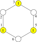
Figure 2: The hexagon lattice of the benzene molecule described by a bipartite Hamiltonian has two equivalent sets of interference points $\mathcal{M}_{I}=\{1,3,5\}$ (yellow) and $\mathcal{M}_{I}=\{2,4,6\}$.

To illustrate the application of these definitions, we find the interference points in the hexagon system, related to the benzene molecule - which is one of the common examples of DQI in single-molecule electron transport [28, 55, 29, 30, 32, 43]. As shown in Fig. 2, this is a bipartite system whose sub-lattice sets are ${\mathcal{M}}_{a}=\{1,3,5\}$ and ${\mathcal{M}}_{b}=\{2,4,6\}$. Since the Hamiltonian matrix is non-singular, from Eq. 8 the two interference sets are ${\mathcal{M}}^{(1)}_{I}={\mathcal{M}}_{a}$ and ${\mathcal{M}}^{(2)}_{I}={\mathcal{M}}_{b}$.

For ${\mathcal{M}}_{I}={\mathcal{M}}_{a}$ we have $G_{n,m}(0)=0,~{}(\forall)~{}n,m\in\{1,3,5\}\,,$ while for ${\mathcal{M}}_{I}={\mathcal{M}}_{b}$, $G_{n,m}(0)=0,~{}(\forall)~{}n,m\in\{2,4,6\}\,.$ The conductance formula from Eq. 7 determines the corresponding transport cancellations.

III General Algorithm

We start from a bipartite lattice with a known interference set $\mathcal{M}_{I}$. The complete set of lattice points $\mathcal{M}$ is therefore decomposed in the reunion of two disjoint subsets,

$${\mathcal{M}}={\mathcal{M}}_{I}\cup{\mathcal{M}}_{R}\,.$$ (9)

where $\mathcal{M}_{R}=\mathcal{M}-\mathcal{M}_{I}$ is by definition the rigid set.

This situation is illustrated in Fig. 3 where the ${\mathcal{M}}_{a}$ sublattice is chosen to be the interference $I$ set (yellow circles) and the remaining ${\mathcal{M}}_{b}$ sublattice is chosen as the rigid $R$ set (empty circles). While it is not mathematically necessary that the $I$ set is identical to $\mathcal{M}_{a}$, such a choice is indicated if one wants to maximize the number of conductance cancelations that are found. The full lines between $I$ and $R$ points correspond to the nonzero hopping energies of the bipartite Hamiltonian.

For the selected $I$ and $R$ lattice points, the Hamiltonian of the bipartite lattice is consequently re-expressed as,

$$H=H(I,R)\,.$$ (10)

The Green’s function matrix for the ${\mathcal{M}_{I}}$ subspace states $G_{II}$ is zero,

$$G_{II}(E)=0\,,$$ (11)

in agreement with Eq. 6. $H$ is perturbed by two additional Hamiltonians, $H_{1}(I)$ which describes the non-zero hopping probabilities among interference points (including onsite new energy terms) and $H_{2}(I,X)$ that contains the hopping elements between the interference points and a set of external points ${\mathcal{M}}_{X}$, as well as any additional $X$-set related terms. The new terms correspond to the dashed lines or to the on-site energies such as $\epsilon_{i}$ and $\epsilon_{x}$ in Fig. 3. The resulting Hamiltonian $H^{\prime}$ is

$$H^{\prime}(I,R,X)=H(I,R)+H_{1}(I)+H_{2}(I,X)\,.$$ (12)

The associated lattice $\mathcal{M^{\prime}}$ described by the Hamiltonian $H^{\prime}$ is the reunion of the three disjoint subsets,

$${\mathcal{M}}^{\prime}={\mathcal{M}}_{I}\cup{\mathcal{M}}_{R}\cup{\mathcal{M}}_{X}\,,$$ (13)

as illustrated in Fig. 3. The original lattice can be grown by adding new points X, such that a conductance cancellation occurs between any point in the $X$ set and any point in the $I$ set. Thus, the conductance cancellations in the enhanced lattice are known apriori by contruction, once the interference set is established.

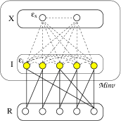
Figure 3: A complex system is built by perturbing the $I$ points from the set ${\mathcal{M}}_{I}$ or by connecting external points $X$ from the set ${\mathcal{M}}_{X}$ to the interference points $I$. The $R$ points are not affected during the construction of the new system. The larger contour enclosing the two sets ${\mathcal{M}}_{X}$ and ${\mathcal{M}}_{I}$ defines the invariance set ${\mathcal{M}}_{inv}$.

We determine the DQI processes in the complex system $H^{\prime}(I,R,X)$ by evaluating the matrix elements of the Green’s function operator $G^{\prime}$. It is assumed that they have no singularities at energy $E$. The Dyson equations satisfied by the matrices $G^{\prime}_{II}$ and $G^{\prime}_{IX}$ are written in terms of the matrix $G_{II}$ as,

$$G^{\prime}_{II}=G_{II}+G_{II}h_{II}G^{\prime}_{II}+G_{II}h_{IX}G^{\prime}_{XI}\;,$$ (14)

$$G^{\prime}_{IX}=G_{II}h_{II}G^{\prime}_{IX}+G_{II}h_{IX}G^{\prime}_{XX}\,,~{}$$ (15)

where $h_{II}$ is the matrix that contains the hopping energies between $I$ sites given by Hamiltonian $H_{1}(I)$ from Eq. 12 and $h_{IX}$ is the matrix that contains the hopping energies between $I$ and $X$ points introduced by the Hamiltonian $H_{2}(I,X)$. We note that the unperturbed Green’s function $G_{IX}$ is zero since the $\mathcal{M}_{I}$ and $\mathcal{M}_{X}$ sets are initially uncoupled.

With $G_{II}(E)=0$ from Eq. 11, Eqs. 14 and 15 generate,

$$G^{\prime}_{II}(E)=0\,,~{}~{}$$ (16)

$$G^{\prime}_{IX}(E)=0\,.~{}~{}$$ (17)

Eq. 16 indicates that ${\mathcal{M}}_{I}$ is a proper interference set for $H^{\prime}$ in agreement with the definition from (6). All the DQI process between the $I$ points are common to both systems described by $H$ and $H^{\prime}$, as shown in Eqs. 11 and 16. The supplementary cancellations in Eq. 17 exhibit the appearance of new DQI processes in the output system between $I$ and $X$ points of the lattice.

The stability of the DQIs is studied with the invariance set,

$${\mathcal{M}}_{\text{inv}}={\mathcal{M}}_{I}\cup{\mathcal{M}}_{X}\,.~{}$$ (18)

The interference points $I$ and the Green’s function zeros, ${G^{\prime}}_{II}$ and ${G^{\prime}}_{IX}$, are not changed by any deformation of $H^{\prime}$ related to ${\mathcal{M}}_{\text{inv}}$ points,

$$H^{\prime}\to H^{\prime}+\sum_{n,m\in{\mathcal{M}}_{\text{inv}}}h_{nm}|n\rangle\langle m|\,.~{}~{}$$ (19)

In Fig. 3 the transformation (19) could represent the modification of hopping energies related to the dashed lines, to the modification of the on-site energies $\epsilon_{i}$ of $I$ points or $\epsilon_{x}$ of $X$ sites. $H^{\prime}$ becomes an effective Hamiltonian when non-hermitian terms, that are introduced to simulate the presence of the external leads attached to the $I$ or $X$ points, are added [56, 51, 57]. In the figure, the ${\mathcal{M}}_{\text{inv}}$ set is shown by the larger contour enclosing $I$ and $X$ points.

From the Green’s functions zeros (16, 17) for the new molecule or physical system we are able to easily predict its conductance zeros when the transport measurements are performed. By connecting the external leads to sites in ${\mathcal{M}}_{I}$, from Eq. 16 one obtains the conductance zeros ${\bf G}_{II}=0$. When the leads are connected to a pair of points, one from ${\mathcal{M}}_{I}$ and the other from $\mathcal{M}_{X}$, from Eq. 17 one obtains ${\bf G}_{IX}=0$. Any system modification according to transformation (19) leaves these conductance zeroes unchanged.

The algorithm discussed here can be applied to various physical or chemical systems that contain embedded sub-systems with known interference sets which undergo the decomposition from Eq. 12 or Fig. 3.

We discuss now the case of a bipartite system for which it is a priory known that $\epsilon=0$ is not an eigenvalue. For such systems any of the sub-lattices $A$ or $B$ can be selected as the ${\cal M}_{I}$ set of points with Green’s function (and conductance) cancellations for any pair of sites between them, including pair of identical sites, as discussed in Section II. Such examples are the circular systems with an even number of atoms which is not a multiple of four and the linear chains with an even number of sites. For the circular molecules we remind that those with $4N$ atoms have a pair of degenerate levels at $\epsilon=0$, which are absent in all other cases [52]. The chain property is trivial [34].

For the hexagonal system in Fig. 2, the general algorithm described above starts by identifying the interference sets. According to Eqs. 8 this bipartite system has two interference sets ${\mathcal{M}}_{I}^{(1)}=\{1,3,5\}$ and ${\mathcal{M}}_{I}^{(2)}=\{2,4,6\}$. The corresponding rigid points sets from Eq. 9 are given by ${\mathcal{M}}-{\mathcal{M}}_{I}$. The two sets are disjointed, so if one is picked as the interference set, by default the other one becomes the rigid set. For ${\mathcal{M}}_{I}^{(1)}=\{1,3,5\}$, ${\mathcal{M}}_{R}^{(1)}=\{2,4,6\}$ and the invariance set from Eq. 18 is obtained to be ${\mathcal{M}}_{\text{inv}}^{(1)}=\{1,3,5\}$ since in this case no external sites were added. Following our theory, diagonal or hopping energies can be added to the ${\mathcal{M}}_{\text{inv}}^{(1)}$ sites without destroying the $I$ points.

The conductance cancellations follow from the $G_{II}$ zeros of the Green’s function. For ${\mathcal{M}}_{I}^{(1)}=\{1,3,5\}$ these conductance zeros are ${\bf G}_{13},{\bf G}_{15}$ and ${\bf G}_{35}$ for the meta-contacted benzene [29, 38], and ${\bf G}_{11}=0,{\bf G}_{33}=0$ and ${\bf G}_{55}=0$ when the two leads are connected to the same point as discussed for the ipso-contacted benzene in [38]. All of these zeros have the invariance set ${\mathcal{M}}_{\text{inv}}^{(1)}=\{1,3,5\}$. For instance the invariance of ${\bf G}_{15}$ at the site $3$ perturbation proves the robustness of the meta-contacted benzene when a heteroatom substitution is performed for real value of $\epsilon_{3}$ [58] or when a third external lead is attached, in this case $\epsilon_{3}$ energy having a complex value [57]. On this line our results may be a support to understand the conductance invariance when heteroatom substitutions in some molecules are performed [59, 54, 60, 61, 58].

We stress that not all lattices have interference sets, even if they may have conductance cancellations (i.e. even if the conductance between $n$ and $m$ is zero, they do not form an interference set unless the conductance is also zero when both leads are connected to $n$ and also when both leads are connected to $m$). The property that a system has an interference set is therefore not trivial, but rather an exception met for instance in bipartite lattices.

IV Extension of the formalism to non-bipartite lattices. The fulvene molecule

In this section we present a complete analysis of the conductance zeros in fulvene, thus augmenting the results of Ref. 44 which studied only several such instances.

To apply the algorithm described in the previous section, we first determine the interference points sets ${\mathcal{M}}_{I}$, as shown in Fig. 4. First, we determine a smaller bipartite system with Hamiltonian $H$ that can provide a set of $I$ points, such that $H=H(I,R)$ is the input Hamiltonian in Eq. 10. Then, the remaining sites and hoppings are added to the $I$ points, generating $H_{add}(I,X)$, such that in the end the complete fulvene Hamiltonian is written as in Eq. 12.

We consider a finite chain of six sites, whose Hamiltonian is $H=\sum|n\rangle\langle n+1|+\text{H.c.}$ with $n=1,\cdots,5$ (hopping energy is set to unity) depicted by straight lines in Fig. 4 (a). This chain is bipartite with $A$ points in the set $\{2,4,6\}$ and $B$ points in the set $\{1,3,5\}$. $H$ is non-singular and satisfies the criteria leading to Eq. 8. We choose $A$ as the interference set, marked with $I$ in the 4 (a). Consequently, the set $B$ contains the rigid points, marked with $R$. To transform the linear chain into the fulvene molecule, a new term that links the $I$ points $2$ and $6$ is added to the Hamiltonian, $H_{add}=|2\rangle\langle 6|+\text{H.c.}$.

Consequently, the fulvene lattice has the interference set ${\mathcal{M}}_{I}^{(a)}=\{2,4,6\}$, the rigid set ${\mathcal{M}}_{R}^{(a)}=\{1,3,5\}$, while the external set from Eq. 13 is empty, ${\mathcal{M}}_{X}^{(a)}=\varnothing$. Figs. 4 (b) and (c) are variants of this scenario without any $X$ points added.

Different decompositions of the total Hamiltonian is presented in Figures 4 (d), (e) and (f) where external points are considered. In Fig. 4 (d), the bipartite system is chosen as $H=\sum|n\rangle\langle n+1|+\text{H.c.}$ with $n=1,\cdots,3$, with $\{2,4\}$ as $A$ points and $\{1,3\}$ as $B$ points. In this case, $H$ is not singular and Eq. 8 is applied. Therefore we choose the $I$ points to be $A$ and $R$ points to be $B$, marked by $I$ and $R$ circles. To recover the full fulvene lattice, two fresh points $X=\{5,6\}$ are added, with new hopping energies represented by dashed lines. $H_{add}$ contains terms that relate the $I$ points to $X$ points, $|2\rangle\langle 6|+|4\rangle\langle 5|+\text{H.c.}$, as well as the hopping between the two $X$ points, $|5\rangle\langle 6|+\text{H.c.}$. The $H_{add}$ is of the type $H_{2}$ in Eq. 12. With this, following the previous results, we obtain that the interference set is ${\mathcal{M}}_{I}^{(d)}=\{2,4\}$, ${\mathcal{M}}_{R}^{(d)}=\{1,3\}$, and ${\mathcal{M}}_{X}^{(d)}=\{5,6\}$. Figs. 4 (e) and (f) represent also new decompositions having $X$ points added.

In Table 1 we give the full list of the six sets of the special points $I$, $R$ and $X$ obtained from the fulvene lattice. It encodes all the $E=0$ DQI processes that exist in the lattice and the corresponding figures explain how they originate from a destructive interference in a bipartite system.

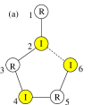
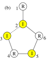
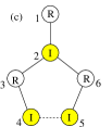
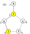
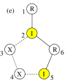
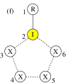
Figure 4: Interference points in fulvene molecule and the decomposition of its lattice sites ${\mathcal{M}}={\mathcal{M}}_{I}\cup{\mathcal{M}}_{R}\cup{\mathcal{M}}_{X}$. $I\in{\mathcal{M}}_{I}$ and $R\in{\mathcal{M}}_{R}$ are the interference and rigid points of the starting bipartite molecule $H_{bip}$ with the lattice points set ${\mathcal{M}}_{bip}={\mathcal{M}}_{I}\cup{\mathcal{M}}_{R}$. In (a)-(f) the dashed lines correspond to the new hopping energies, while the $X$ circles in (d)-(f) designate the new external sites ${\mathcal{M}}_{X}$ added to the initial bipartite molecule (composed of $I$ and $R$ circles).

Table 1: Fulvene special points: interference points $I$, rigid points $R$ and external points $X$. $I\in{\mathcal{M}}_{I}$, $R\in{\mathcal{M}}_{R}$ and $X\in{\mathcal{M}}_{X}$. The robustness of every interference set ${\mathcal{M}}_{I}$ is dictated by the invariance set ${\mathcal{M}}_{\text{inv}}={\mathcal{M}}_{I}\cup{\mathcal{M}}_{X}$.

Fig. 4	Interference	Rigid	External
	points $I$	points $R$	points $X$
(a)	2, 4, 6	1, 3, 5
(b)	2, 3, 5	1, 4, 6
(c)	2, 4, 5	1, 3, 6
(d)	2, 4	1, 3	5, 6
(e)	2, 5	1, 6	3, 4
(f)	2	1	3, 4, 5, 6

Table 2: The twelve DQI processes at $E=0$ for the fulvene lattice and their invariance sets.

Green’s function	Invariance
zeros	at ${\mathcal{M}}_{\text{inv}}$
$G_{22},G_{23},G_{24},$	${\mathcal{M}}_{\text{inv}}^{(f)}=\{{2},{3},{4},{5},{6}\}$
$G_{25},G_{26}$
$G_{44},G_{46}$	${\mathcal{M}}_{\text{inv}}^{(d)}=\{2,4,5,6\}$
$G_{55},G_{35}$	${\mathcal{M}}_{\text{inv}}^{(e)}=\{2,3,4,5\}$
$G_{33}$	${\mathcal{M}}_{\text{inv}}^{(b)}=\{2,3,5\}$
$G_{66}$	${\mathcal{M}}_{\text{inv}}^{(a)}=\{2,4,6\}$
$G_{45}$	${\mathcal{M}}_{\text{inv}}^{(d)}=\{2,4,5,6\}$
	${\mathcal{M}}_{\text{inv}}^{(e)}=\{2,3,4,5\}$

Different choices of the initial set of interference points lead to different predictions of zeros of conductances and to various invariance sets. It is therefore important that one finds all the possible zeros together with there invariance sets, as summarized in Table 2.

We remark that when compared with all the other conductance zeros that are associated with a single invariance set, the $G_{45}$ zero is associated with two. From Figs. 4 (c), (d) and (e) or from the corresponding lines of the Table 1, we note that $G_{45}$ is a $G_{II}$ zero in (c) and a $G_{IX}$ zero in (d) and (e). The three invariance sets of $G_{45}$ zero are, ${\cal M}^{(c)}_{\text{inv}}=\{2,4,5\}$, ${\cal M}^{(d)}_{\text{inv}}=\{2,4,5,6\}$ and ${\cal M}^{(e)}_{\text{inv}}=\{2,3,4,5\}$. The set ${\cal M}^{(c)}_{\text{inv}}$ can be ignored as it is included in the others two sets and one retains only two invariance sets, ${\cal M}^{(d)}_{\text{inv}}$ and ${\cal M}^{(e)}_{\text{inv}}$.

Another matter of interest is to say not only which perturbations keep the conductance zeros invariant but also which ones lift them leading to nonzero current through a given molecular device [62, 35, 57]. Since we have shown that the conductance zeros are invariant under the $I$ and $X$ sites perturbations it can be assumed that they may be destroyed by means of $R$ sites. This however has to be investigated for every particular case.

It is straightforward to show that in the case of a small molecule like fulvene, the conductance zeroes can be individually predicted by alternative approaches, such as the four graphs nullities investigation [38], determinant algorithm [40, 45] or by direct calculation from the power series expansion of the Green’s function [44]. We believe that our method becomes more practical when large molecules or large lattices are involved. Then, once at least one bipartite sub-system is found, conductance zeroes can be predicted in group rather than individually, along with their robustness under perturbations.

V Conclusions

In this paper, we develop a method for determining the conductance zeros that result from destructive electron state interference in complex systems. The method starts by finding a smaller system which includes an interference set, whose points are such that any pair of them is associated with zero conductance (${\bf G}_{II}=0$, including the diagonal terms, when both leads are connected to the same site). The remaining points from this initial system, outside the interference set, are called rigid points $R$. A complex system is then obtained by connecting new, external points $X$ to the $I$ points (but never to the $R$ points) or by adding any on-site or hopping energies related to the $I$ points. We prove that the new system obtained in this way retains all the initial conductance cancellations between the $I$ points (${\bf G}_{II}=0$) and, in addition, exhibits new zeros between points $I$ and points $X$ (${\bf G}_{IX}=0$).

Bipartite systems are known to have such sets of interference points at zero energy, provided that $\epsilon=0$ is not an eigenvalue of the system (i.e. Hamiltonian is non-singular), and they are used as starting blocks in our derivations. In such a case, the sets of $I$ points can be identified with the sub-lattices points A or B. Among the simplest examples of bipartite systems with non-singular Hamiltonians we mention the linear chains with $2N$ sites and circular molecules with $4N+2$ sites.

The Dyson expansion is used to prove the conductance cancelations as well as their invariance properties. The zeros are robust against perturbations applied on the $I$ and $X$ points, while the $R$ points should not be perturbed.

In the case of the non-bipartite fulvene molecule it is shown that, by choosing in different ways the initial set of $I$ points, one can obtain all the conductance zeros and study their persistence under the effect of different perturbations.

Our study contributes to the understanding of the destructive interferences and their invariance properties for an appropriate class of physical systems that have bipartite lattices or contain subsystems with bipartite lattices. They can be relevant for transport experiments on molecules, nanostructures and various finite lattices, for designing of logical gates or for projection of quantum interference transistors at the nanoscale.

Appendix A Conductance Calculation

In this Section we briefly remind how the Green’s function cancellations reflect also in the conductance, should the system no longer be isolated, but connected to external leads. Let us consider for this a two-terminal conductor, such as a tight-binding lattice connected at two semi-infinite leads called $L_{out}$ and $L_{in}$. They are coupled at two sites of the involved lattice $i$ and $j$, respectively. Transport coefficients are given in terms of the effective Green’s function of the Hamiltonian $H^{\text{eff}}=H+\tau_{i}|i\rangle\langle i|+\tau_{j}|j\rangle\langle j|$. This is evaluated as in Refs. 51, 56 for a wave vector $k$ and Fermi energy $E=2\tau_{l}\cos k$ as a function of $\tau_{l}$, the hopping energy on the leads, and $\tau_{c}$, the hopping energy between the leads and the discrete system. Therefore,

$${G}^{\text{eff}}_{ij}(E)=\frac{{G}_{ij}(E)}{1-\tau_{j}{G}_{jj}-\tau_{i}{G}_{ii}-\tau_{j}\tau_{i}{G}_{ij}{G}_{ji}+\tau_{j}\tau_{i}{G}_{ii}{G}_{jj}}\;,$$

$$\text{with}~{}\tau_{i,j}=\frac{\tau_{c}^{2}}{\tau_{l}}e^{-ik}.$$ (20)

In the Landauer-Büttiker approach [63, 64, 65] the tunneling amplitude from the lead $L_{in}$ into the lead $L_{out}$ gives the scattered wave function in the lead $L_{out}$, $|\Psi_{L_{out}}\rangle={\bf t}_{out,in}\sum_{n_{l}\in L_{out}}e^{-ikn_{l}}|n_{l}\rangle$. The tunnelig amplitude from $L_{in}$ to $L_{out}$ is

$${\bf t}_{out,in}(E)=2i\frac{\tau_{c}^{2}}{\tau_{l}}\sin k\;{G}^{\text{eff}}_{ij}(E)\,.$$ (21)

The electric conductance ${\bf G}_{ij}$ or transmittance ${\bf T}_{ij}$ are given:

$${\bf G}_{ij}(E)=\frac{e^{2}}{h}{\bf T}_{ij}(E)=\frac{e^{2}}{h}|{\bf t}_{out,in}(E)|^{2}\,.$$ (22)

Straightforwardly, the effective Green’s function ${G}^{\text{eff}}_{ij}(E)$ and of course the conductance ${\bf G}_{ij}(E)$ cancels whenever the Green’s function of the isolated sample ${G}_{ij}(E)$ is equal to zero.

We also point out again that the Green’s function cancellations obtained in Eqs. 16 and 17 are proved for nonsingular $H^{\prime}$ such that $G^{\prime}$ Green’s functions in Dyson expansions from Eqs. 14 and 15 have no singularities at energy $E$. Otherwise, supplementary calculations have to be carried out, by using for instance effective Hamiltonian depicted here, to directly prove the conductance cancellations. With some exception (as the square Hamiltonian in [31]) $H^{\text{eff}}$ is nonsingular because of the non-hermitian terms added to the contact points.

References

- Aharonov and Bohm [1959] Y. Aharonov and D. Bohm, Significance of electromagnetic potentials in the quantum theory, Phys. Rev. 115, 485 (1959).
- Hod et al. [2008] O. Hod, R. Baer, and E. Rabani, Magnetoresistance of nanoscale molecular devices based on Aharonov-Bohm interferometry, Journal of Physics: Condensed Matter 20, 383201 (2008).
- Imry [2008] Y. Imry, Introduction in mesoscopic physics (Oxford University Press, 2008).
- Lee [1999] H.-W. Lee, Generic transmission zeroes and in-phase resonances in time-reversal symmetric single channel transport, Phys. Rev. Lett 82, 2358 (1999).
- Rincón et al. [2009] J. Rincón, K. Hallberg, A. A. Aligia, and S. Ramasesha, Quantum interference in coherent molecular conductance, Phys. Rev. Lett. 103, 266807 (2009).
- Sparks et al. [2011] R. E. Sparks, V. M. García-Suárez, D. Z. Manrique, and C. J. Lambert, Quantum interference in single molecule electronic systems, Phys. Rev. B 83, 075437 (2011).
- Hsu and Rabitz [2012] L.-Y. Hsu and H. Rabitz, Single-molecule phenyl-acetylene-macrocycle-based optoelectronic switch functioning as a quantum-interference-effect transistor, Phys. Rev. Lett. 109, 186801 (2012).
- Lambert [2015] C. J. Lambert, Basic concepts of quantum interference and electron transport in single-molecule electronics, Chem. Soc. Rev. 44, 875 (2015).
- Pedersen et al. [2015] K. G. L. Pedersen, A. Borges, P. Hedegård, G. C. Solomon, and M. Strange, Illusory connection between cross-conjugation and quantum interference, The Journal of Physical Chemistry C 119, 26919 (2015), https://doi.org/10.1021/acs.jpcc.5b10407 .
- Tsuji et al. [2016] Y. Tsuji, R. Hoffmann, M. Strange, and G. C. Solomon, Close relation between quantum interference in molecular conductance and diradical existence, Proceedings of the National Academy of Sciences 113, E413 (2016), https://www.pnas.org/content/113/4/E413.full.pdf .
- Su et al. [2016] T. A. Su, M. Neupane, M. L. Steigerwald, L. Venkataraman, and C. Nuckolls, Chemical principles of single-molecule electronics, Nature Reviews Materials 1, 16002 EP (2016), review Article.
- Zhao et al. [2017] X. Zhao, V. Geskin, and R. Stadler, Destructive quantum interference in electron transport: A reconciliation of the molecular orbital and the atomic orbital perspective, The Journal of Chemical Physics 146, 092308 (2017), https://doi.org/10.1063/1.4972572 .
- Zhang et al. [2018] Y. Zhang, G. Ye, S. Soni, X. Qiu, T. Krijger, H. T. Jonkman, M. Carlotti, E. Sauter, M. Zharnikov, and R. C. Chiechi, Controlling destructive quantum interference in tunneling junctions comprising self-assembled monolayers via bond topology and functional groups, Chem. Sci. 9, 4414 (2018).
- Liu et al. [2019] J. Liu, X. Huang, F. Wang, and W. Hong, Quantum interference effects in charge transport through single-molecule junctions: Detection, manipulation, and application, Accounts of Chemical Research 52, 151 (2019), https://doi.org/10.1021/acs.accounts.8b00429 .
- Lambert and Liu [2018] C. J. Lambert and S.-X. Liu, A magic ratio rule for beginners: A chemist’s guide to quantum interference in molecules, Chemistry – A European Journal 24, 4193 (2018).
- Mijbil [2019] Z. Y. Mijbil, Quantum interference independence of the heteroatom position, Chemical Physics Letters 716, 69 (2019).
- Xin et al. [2019] N. Xin, J. Guan, C. Zhou, X. Chen, C. Gu, Y. Li, M. A. Ratner, A. Nitzan, J. F. Stoddart, and X. Guo, Concepts in the design and engineering of single-molecule electronic devices, Nature Reviews Physics 1, 211 (2019).
- Li et al. [2019a] Y. Li, M. Buerkle, G. Li, A. Rostamian, H. Wang, Z. Wang, D. R. Bowler, T. Miyazaki, L. Xiang, Y. Asai, G. Zhou, and N. Tao, Gate controlling of quantum interference and direct observation of anti-resonances in single molecule charge transport, Nature Materials 18, 357 (2019a).
- Li et al. [2019b] D. Li, R. Banerjee, S. Mondal, I. Maliyov, M. Romanova, Y. J. Dappe, and A. Smogunov, Symmetry aspects of spin filtering in molecular junctions: Hybridization and quantum interference effects, Phys. Rev. B 99, 115403 (2019b).
- Gunasekaran et al. [2020] S. Gunasekaran, J. E. Greenwald, and L. Venkataraman, Visualizing quantum interference in molecular junctions, Nano Lett. 20, 2843 (2020).
- Li et al. [2019c] Y. Li, X. Yu, Y. Zhen, H. Dong, and W. Hu, Two-pathway viewpoint to interpret quantum interference in molecules containing five-membered heterocycles: Thienoacenes as examples, J. Phys. Chem. C 123, 15977 (2019c).
- Levy Yeyati and Büttiker [2000] A. Levy Yeyati and M. Büttiker, Scattering phases in quantum dots: An analysis based on lattice models, Phys. Rev. B 62, 7307 (2000).
- Niţă et al. [2020] M. Niţă, M. Ţolea, and D. C. Marinescu, Robust conductance zeros in graphene quantum dots and other bipartite systems, Phys. Rev. B 101, 235318 (2020).
- Rotter and Sadreev [2005] I. Rotter and A. F. Sadreev, Zeros in single-channel transmission through double quantum dots, Phys. Rev. E 71, 046204 (2005).
- Tada and Yoshizawa [2002] T. Tada and K. Yoshizawa, Quantum transport effects in nanosized graphite sheets, ChemPhysChem 3, 1035 (2002).
- Niţă et al. [2014] M. Niţă, M. Ţolea, and B. Ostahie, Transmission phase lapses at zero energy in graphene quantum dots, physica status solidi (RRL) – Rapid Research Letters 08, 790 (2014).
- Valli et al. [2019] A. Valli, A. Amaricci, V. Brosco, and M. Capone, Interplay between destructive quantum interference and symmetry-breaking phenomena in graphene quantum junctions, Phys. Rev. B 100, 075118 (2019).
- Sautet and Joachim [1988] P. Sautet and C. Joachim, Electronic interference produced by a benzene embedded in a polyacetylene chain, Chemical Physics Letters 153, 511 (1988).
- Nozaki and Toher [2017a] D. Nozaki and C. Toher, Is the antiresonance in meta-contacted benzene due to the destructive superposition of waves traveling two different routes around the benzene ring?, The Journal of Physical Chemistry C 121, 11739 (2017a).
- Sýkora and Novotný [2017a] R. Sýkora and T. Novotný, Comment on “is the antiresonance in meta-contacted benzene due to the destructive superposition of waves traveling two different routes around the benzene ring”, J. Phys. Chem. C 121, 19538 (2017a).
- Sýkora and Novotný [2017b] R. Sýkora and T. Novotný, Graph-theoretical evaluation of the inelastic propensity rules for molecules with destructive quantum interference, The Journal of Chemical Physics 146, 174114 (2017b), https://doi.org/10.1063/1.4981916 .
- Nozaki and Toher [2017b] D. Nozaki and C. Toher, Is the antiresonance in meta-contacted benzene due to the destructive superposition of waves traveling two different routes around the benzene ring?, The Journal of Physical Chemistry C 121, 19540 (2017b).
- Pedersen et al. [2014] K. G. L. Pedersen, M. Strange, M. Leijnse, P. Hedegård, G. C. Solomon, and J. Paaske, Quantum interference in off-resonant transport through single molecules, Phys. Rev. B 90, 125413 (2014).
- Tsuji et al. [2014] Y. Tsuji, R. Hoffmann, R. Movassagh, and S. Datta, Quantum interference in polyenes, The Journal of Chemical Physics 141, 224311 (2014), https://doi.org/10.1063/1.4903043 .
- Chen et al. [2018] S. Chen, G. Chen, and M. A. Ratner, Designing principles of molecular quantum interference effect transistors, The Journal of Physical Chemistry Letters 9, 2843 (2018), pMID: 29750871, https://doi.org/10.1021/acs.jpclett.8b01185 .
- Miroshnichenko et al. [2010] A. E. Miroshnichenko, S. Flach, and Y. S. Kivshar, Fano resonances in nanoscale structures, Rev. Mod. Phys. 82, 2257 (2010).
- Nozaki et al. [2013] D. Nozaki, H. Sevinçli, S. M. Avdoshenko, R. Gutierrez, and G. Cuniberti, A parabolic model to control quantum interference in T-shaped molecular junctions, Phys. Chem. Chem. Phys. 15, 13951 (2013).
- Fowler et al. [2009] P. W. Fowler, B. T. Pickup, T. Z. Todorova, and W. Myrvold, A selection rule for molecular conduction, J. Chem. Phys. 131, 044104 (2009).
- Mayou et al. [2013] D. Mayou, Y. Zhou, and M. Ernzerhof, The zero-voltage conductance of nanographenes: Simple rules and quantitative estimates, J. Phys. Chem. C 117, 7870 (2013).
- Markussen et al. [2010] T. Markussen, R. Stadler, and K. S. Thygesen, The relation between structure and quantum interference in single molecule junctions, Nano Letters 10, 4260 (2010), pMID: 20879779, https://doi.org/10.1021/nl101688a .
- Reuter and Hansen [2014] M. G. Reuter and T. Hansen, Communication: Finding destructive interference features in molecular transport junctions, The Journal of Chemical Physics 141, 181103 (2014), https://doi.org/10.1063/1.4901722 .
- Stuyver et al. [2015] T. Stuyver, F. Stijn, F. De Proft, and G. Paul, Back of the envelope selection rule for molecular transmission: A curly arrow approach, J. Phys. Chem. C 119, 26390 (2015).
- Sam-ang and Reuter [2017] P. Sam-ang and M. G. Reuter, Characterizing destructive quantum interference in electron transport, New Journal of Physics 19, 053002 (2017).
- Tsuji et al. [2018] Y. Tsuji, E. Estrada, R. Movassagh, and R. Hoffmann, Quantum interference, graphs, walks, and polynomials, Chemical Reviews 118, 4887 (2018), pMID: 29630345, https://doi.org/10.1021/acs.chemrev.7b00733 .
- Evers et al. [2020] F. Evers, R. Korytár, S. Tewari, and J. M. van Ruitenbeek, Advances and challenges in single-molecule electron transport, Reviews of Modern Physics 92, 035001 (2020).
- Dhakal and Rai [2019] U. Dhakal and D. Rai, Tight-binding model of graphene nanosheets, Physics Letters A 383, 2193 (2019).
- Tamura et al. [2002] H. Tamura, K. Shiraishi, T. Kimura, and H. Takayanagi, Flat-band ferromagnetism in quantum dot superlattices, Phys. Rev. B 65, 085324 (2002).
- Norimoto and Nakamura [2018] S. Norimoto and S. Nakamura, Fano effect in the transport of an artificial molecule, Phys. Rev. B 97, 195313 (2018).
- Coulson and Rushbrooke [1940] C. A. Coulson and G. S. Rushbrooke, Note on the method of molecular orbitals, Mathematical Proceedings of the Cambridge Philosophical Society 36, 193–200 (1940).
- Deng and Wakabayashi [2014] H.-Y. Deng and K. Wakabayashi, Edge effect on a vacancy state in semi-infinite graphene, Phys. Rev. B 90, 115413 (2014).
- Ostahie et al. [2016] B. Ostahie, M. Niţă, and A. Aldea, Non-Hermitian approach of edge states and quantum transport in a magnetic field, Phys. Rev. B 94, 195431 (2016).
- Niţă et al. [2017] M. Niţă, M. Ţolea, D. C. Marinescu, and A. Manolescu, Hund and anti-Hund rules in circular molecules, Phys. Rev. B 96, 235101 (2017).
- Koshino et al. [2014] M. Koshino, T. Morimoto, and M. Sato, Topological zero modes and Dirac points protected by spatial symmetry and chiral symmetry, Phys. Rev. B 90, 115207 (2014).
- Tsuji and Yoshizawa [2017] Y. Tsuji and K. Yoshizawa, Frontier orbital perspective for quantum interference in alternant and nonalternant hydrocarbons, The Journal of Physical Chemistry C 121, 9621 (2017), https://doi.org/10.1021/acs.jpcc.7b02274 .
- Patoux et al. [1997] C. Patoux, C. Coudret, J.-P. Launay, C. Joachim, and A. Gourdon, Topological effects on intramolecular electron transfer via quantum interference, Inorganic Chemistry 36, 5037 (1997), https://doi.org/10.1021/ic970013m .
- Ţolea et al. [2010] M. Ţolea, M. Niţă, and A. Aldea, Analyzing the measured phase in the multichannel Aharonov-Bohm interferometer, Physica E: Low-dimensional Systems and Nanostructures 42, 2231 (2010).
- Cardamone et al. [2006] D. M. Cardamone, C. A. Stafford, and S. Mazumdar, Controlling quantum transport through a single molecule, Nano Lett. 6, 2426 (2006).
- Sangtarash et al. [2018] S. Sangtarash, H. Sadeghi, and C. J. Lambert, Connectivity-driven bi-thermoelectricity in heteroatom-substituted molecular junctions, Phys. Chem. Chem. Phys. 20, 9630 (2018).
- Garner et al. [2016] M. H. Garner, G. C. Solomon, and M. Strange, Tunning conductance in aromatic molecules: Constructive and counteractive substituent effects, J Phys. Chem. C 120, 9097 (2016).
- Tsuji et al. [2017] Y. Tsuji, T. Stuyver, S. Gunasekaran, and L. Venkataraman, The influence of linkers on quantum interference: A linker theorem, J Phys. Chem. C 121, 14451 (2017).
- Liu et al. [2017] X. Liu, S. Sangtarash, D. Reber, D. Zhang, H. Sadeghi, J. Shi, Z.-Y. Xiao, W. Hong, C. J. Lambert, and S.-X. Liu, Gating of quantum interference in molecular junctions by heteroatom substitution, Angewandte Chemie International Edition 56, 173 (2017).
- Baer and Neuhauser [2002] R. Baer and D. Neuhauser, Anti-coherence based molecular electronics: Xor-gate response, Chemical Physics 281, 353 (2002).
- Landauer [1957] R. Landauer, Spatial variation of currents and fields due to localized scatterers in metallic conduction, IBM Journal of Research and Development 1, 223 (1957).
- Büttiker [1986] M. Büttiker, Four-terminal phase-coherent conductance, Phys. Rev. Lett 57, 1761 (1986).
- Imry and Landauer [1999] Y. Imry and R. Landauer, Conductance viewed as transmission, Rev. Mod. Phys. 71, S306 (1999).