Self-supervised Discriminative Feature Learning for Deep Multi-view Clustering

Abstract

Multi-view clustering is an important research topic due to its capability to utilize complementary information from multiple views. However, there are few methods to consider the negative impact caused by certain views with unclear clustering structures, resulting in poor multi-view clustering performance. To address this drawback, we propose self-supervised discriminative feature learning for deep multi-view clustering (SDMVC). Concretely, deep autoencoders are applied to learn embedded features for each view independently. To leverage the multi-view complementary information, we concatenate all views’ embedded features to form the global features, which can overcome the negative impact of some views’ unclear clustering structures. In a self-supervised manner, pseudo-labels are obtained to build a unified target distribution to perform multi-view discriminative feature learning. During this process, global discriminative information can be mined to supervise all views to learn more discriminative features, which in turn are used to update the target distribution. Besides, this unified target distribution can make SDMVC learn consistent cluster assignments, which accomplishes the clustering consistency of multiple views while preserving their features’ diversity. Experiments on various types of multi-view datasets show that SDMVC achieves state-of-the-art performance. The code is available at https://github.com/SubmissionsIn/SDMVC.

I Introduction

AS a fundamental task, clustering analysis has been applied in a wide range of fields, such as machine learning, computer vision, data mining, and pattern recognition, etc. However, traditional clustering methods are generally inapplicable in the scenarios where the real-world data are collected from multiple views or modalities, e.g., (1) multiple mappings of one object, (2) visual feature + textual feature, (3) scale-invariant feature transform (SIFT) + local binary pattern (LBP). Therefore, multi-view clustering (MVC) becomes a hot research topic that can access complementary information and comprehensive characteristics hidden in multi-view data.

MVC can be roughly classified into four categories: (1) Numerous MVC methods are based on subspace clustering [1, 2, 3, 4], where the shared representation of multiple views and similarity metric matrix are explored. (2) Some MVC methods [5, 6, 7] apply non-negative matrix factorization to decompose each view into a low-rank matrix for clustering. (3) In the third MVC category [8, 9, 10], graph-based structure information is integrated to mine clusters among multiple views. (4) Deep learning techniques are also applied to MVC in recent years, such as [11, 12, 13, 14, 15]. Deep MVC aims to obtain better performance with the feature representation capability of deep models. More details can be found in [16, 17] which provide a comprehensive survey about multi-view clustering.

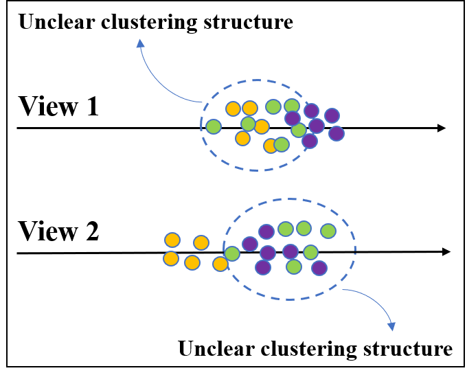
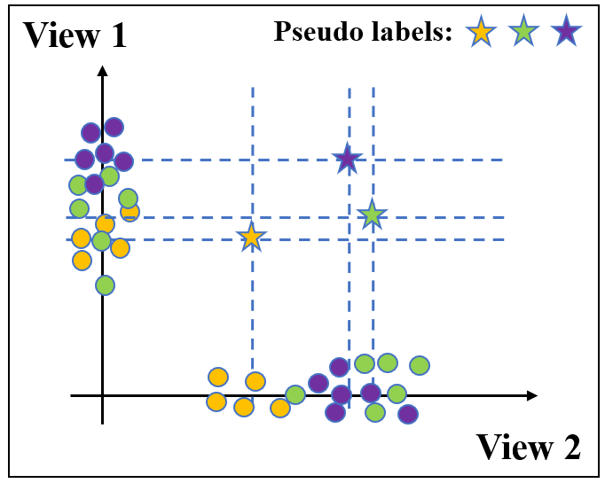
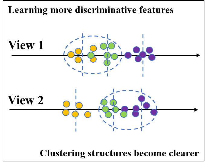
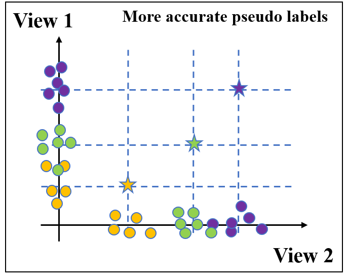
Figure 1: An illustrative example of our motivation.

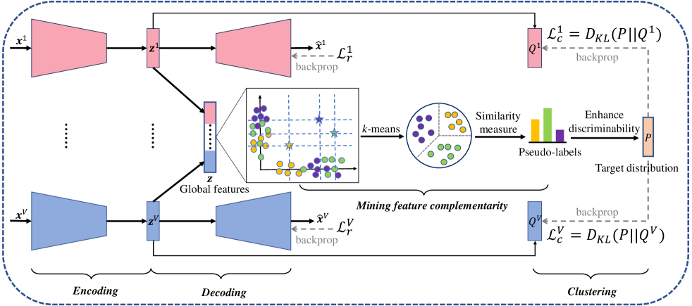
Figure 2: The framework of SDMVC. Each view contains an autoencoder an a clustering layer. $\boldsymbol{z}^{v}$ is the embedded features and $Q^{v}$ is the cluster assignment distribution. The unified target distribution $P$ is iteratively updated to conduct multi-view discriminative feature learning.

Although existing MVC methods have achieved significant progress in the past decade, their performance is still limited in the following issues. Firstly, some MVC methods depend on too many hyper-parameters. But in a real clustering application, there is no label information that can be used to tune them. Besides, many MVC methods have suffered from high complexity, so they are difficult to solve large-scale data clustering tasks. In addition, previous works usually conduct the consistency of multiple views directly in the embedded feature space, which reduces the capability of features to preserve the diversity among multiple views. The consequence is, if certain views’ clustering structures are highly fuzzy, the effect of the views with clear clustering structures will be limited and thus results in poor clustering performance.

To overcome the aforementioned issues, we propose self-supervised discriminative feature learning for deep multi-view clustering (SDMVC). Our motivation comes from the observation illustrated in Fig. 1: (a) The discriminability of multiple views is different due to their diversity (for example, red motorcycles and red bicycles are almost indistinguishable from a color view, but they are clearly distinguishable from a semantic view). So, the discriminative degree of different views’ features are different and higher discriminative features are more conducive to clustering (i.e., higher discriminative features have clearer clustering structures). (b) When the features are concatenated, the clustering structures with high discriminability play a major role in dividing the global feature space, which can produce pseudo-labels of high confidence and overcome the negative effects of unclear clustering structures. (c) – (d) The pseudo-labels can be used to lead all views to learn more discriminative features, which further produce clearer clustering structures and more accurate pseudo-labels.

Specially, the proposed self-supervised multi-view discriminative feature learning framework is shown in Fig. 2. For each view, a corresponding autoencoder is employed to learn low-dimensional embedded features $\boldsymbol{z}^{v}$ by optimizing the reconstruction loss $\mathcal{L}_{r}^{v}$. The discriminability of different views’ embedded features is different. To leverage the global discriminative information, we concatenate all embedded features to build global features, pseudo-labels, and a unified target distribution, in sequence. During this process, the feature complementarity can be mined and the negative effects of the views with unclear clustering structures can be overcome. Then, the feature learning is performed by optimizing the KL divergence $\mathcal{L}_{c}^{v}$ between the unified target distribution $P$ and each view’s cluster assignments $Q^{v}$. In this way, global discriminative information can be used to lead all views to learn more discriminative features, which in turn help to obtain complementary information and a more accurate target distribution. We further prove that SDMVC can learn consistent cluster assignments, i.e., accomplish the clustering consistency of all views by optimizing the multi-view clustering loss with the proposed unified target distribution. Besides, the framework can preserve the diversity of all views’ features due to the proposed independent training for each view.

In summary, the contributions of this paper include:

• We propose a deep MVC method with a novel self-supervised multi-view discriminative feature learning framework, which can leverage the global discriminative information contained in all views’ embedded features to perform multi-view clustering.

• From the perspective of cluster assignments rather than features, the proposed framework implements the clustering consistency of multiple views while preserving their features’ diversity. In addition, it can overcome the negative impact on multi-view clustering caused by some views with unclear clustering structures.

• The proposed method does not depend on certain hyper-parameters and its complexity is linear to the data size. Experiments on different types of datasets demonstrate its state-of-the-art clustering performance.

II Related Work

II-A Deep Embedded Clustering

Deep autoencoder, one of the popular deep models, has good embedded feature representation capability and its computing complexity is linear to data size. Recently, deep autoencoder based clustering has been extensively studied. One of the most popular works is deep embedded clustering (DEC) [18], which jointly learns the cluster assignments and embedded features of autoencoders. The improved deep embedded clustering (IDEC) [19] introduced a trade-off between clustering and reconstruction to prevent the collapse of embedded space. The model proposed in [20] is another variant of DEC which stacks multinomial logistic regression on top of a convolutional autoencoder. More researches based on DEC can be found in [21, 22, 23]. Although many works based on deep neural network has achieved impressive performance [18, 20, 24, 25], those methods can not handle multi-view clustering tasks. In this paper, we propose a novel deep multi-view clustering framework where discriminative embedded features are learned in a self-supervised manner.

II-B Multi-view Clustering

Subspace-based multi-view clustering is widely discussed, which assumes that the data of multiple views come from a same latent space. In [26], the authors explored self-representation layers to reconstruct view-specific subspace hierarchically and encoding layers to make cross-view subspace more consensus. Recently, in [13] and [27], multi-view data was transformed into a joint representation to perform multi-view clustering. Another work [28] learned multi-view embeddings and jointly mined common structure and cluster assignments in the learned latent space. Some multi-view clustering methods were implemented by using non-negative matrix factorization techniques, e.g., by which Liu et al. [5] explored a common latent factor among multiple views. A deep structure [29] was built to seek common features with more consistent information. Some methods [8, 9, 30, 31, 32] exploited graph-based models for multi-view clustering. For example, a multi-graph laplacian regularized low-rank representation was proposed in [33] for multi-view spectral clustering. Peng et al. [10] mined geometry and cluster alignment consistency in projection space by connection graph. In [34], graph autoencoders were also introduced to learn multi-view representation.

Some works are based on other learning approaches. For instance, Zhang et al. [35] incorporated discrete representation learning and binary clustering into a unified framework. In [36], self-paced learning was applied to prevent being stuck in local optima. In addition, deep learning is an attention-getting trend. For example, Zhu et al. [12] trained deep autoencoders to obtain self-representation and leveraged the diversity and universality regularization to abstract higher-order relation among views. Adversarial learning based deep MVC was proposed in [11, 37], which aim to learn the intrinsic embedded structure of multi-view data. Self-supervised learning is the recent hot topic of the community. The framework proposed in [38] combined a self-supervised paradigm with multi-view clustering. However, it belongs to subspace clustering and depends on the eigenvalue decomposition, which causing cubic complexity to the data size.

For multi-view clustering, it is important to obtain consistent predictions of multiple views for the same examples. Wang et al. [39] maximized the alignment between weighted view-specific partition and consensus partition. The referred view was introduced in [14] to explicitly train all views to achieve consistent predictions. The latest work [40] introduced two deep MVC models when aligning the distributions of multi-view representations. Unlike previous methods, our approach achieves consistent multi-view clustering predictions by establishing a unified target distribution. Besides, the self-supervised multi-view discriminative feature learning framework is first proposed in our work.

III The Proposed Method

Problem Statement. Given a multi-view dataset $\{\boldsymbol{x}^{1}_{i}\in\mathbb{R}^{D_{1}},\boldsymbol{x}^{2}_{i}\in\mathbb{R}^{D_{2}},\dots,\boldsymbol{x}^{V}_{i}\in\mathbb{R}^{D_{V}}\}_{i=1}^{N}$, $V$ is the total number of views, $N$ is the number of examples, and $D_{1},D_{2},\dots,D_{V}$ are the dimensionality of views. Multi-view clustering aims to partition the examples into $K$ clusters.

III-A Self-supervised Multi-view Discriminative Feature Learning

Generally, multiple views of an example are different in dimension or input form. In order to obtain the features that are convenient to clustering, we use deep autoencoders to perform feature representation learning for each view. Specifically, let $f_{\theta^{v}}^{v}$ and $g_{\phi^{v}}^{v}$ represent the encoder and decoder of the $v$-th view, respectively. The parameters $\theta^{v}$ and $\phi^{v}$ implement the nonlinear mapping of the $v$-th autoencoder, whose encoder part learn the low-dimensional features by

$$\boldsymbol{z}_{i}^{v}=f^{v}_{\theta^{v}}{(\boldsymbol{x}_{i}^{v})},$$ (1)

where $\boldsymbol{z}_{i}^{v}\in\mathbb{R}^{d_{v}}$ is the embedded point of $\boldsymbol{x}_{i}^{v}$ in $d_{v}$-dimensional feature space. The decoder part of autoencoder reconstructs the example as $\hat{\boldsymbol{x}}_{i}^{v}\in\mathbb{R}^{D_{v}}$ by decoding $\boldsymbol{z}_{i}^{v}$:

$$\hat{\boldsymbol{x}}_{i}^{v}=g^{v}_{\phi^{v}}{(\boldsymbol{z}_{i}^{v})}=g^{v}_{\phi^{v}}{(f^{v}_{\theta^{v}}{(\boldsymbol{x}_{i}^{v})})}.$$ (2)

For each view, the reconstruction loss between input and output is optimized, so as to transform the input of various forms into low-dimensional embedded features:

$$\mathcal{L}_{r}^{v}=\sum_{i=1}^{N}\left\|{\boldsymbol{x}_{i}^{v}-g^{v}_{\phi^{v}}{(f^{v}_{\theta^{v}}{(\boldsymbol{x}_{i}^{v})})}}\right\|_{2}^{2}.$$ (3)

On the top of each view’s embedded features, we construct a clustering layer $c^{v}_{\mu^{v}}$ with learnable parameters $\{\boldsymbol{\mu}_{j}^{v}\in\mathbb{R}^{d_{v}}\}_{j=1}^{K}$. $\boldsymbol{\mu}_{j}^{v}$ represents the $j$-th cluster centroid of the $v$-th view. Additionally, DEC [18] and IDEC [19] are popular single-view deep clustering methods which apply Student’s $t$-distribution [41] to generate soft cluster assignments. The similar way is applied to calculate our clustering layer’s output, which can be described as:

$$q_{ij}^{v}=c^{v}_{\mu^{v}}{(\boldsymbol{z}_{i}^{v})}=\frac{(1+\lVert\boldsymbol{z}_{i}^{v}-\boldsymbol{\mu}_{j}^{v}\rVert^{2})^{-1}}{\sum_{j}(1+\lVert\boldsymbol{z}_{i}^{v}-\boldsymbol{\mu}_{j}^{v}\rVert^{2})^{-1}},$$ (4)

where $q_{ij}^{v}$ is the probability (soft cluster assignment) that the $i$-th example belongs to the $j$-th cluster in the $v$-th view. As shown in Fig. 2, our framework has $V$ clustering layers and $V$ autoencoders. All view’s embedded features are learned independently, which is essential to learn each view’s special characteristics that can provide complementary information for multi-view clustering.

Actually, the soft assignments calculated by Eq. (4) measure the similarity between embedded features and cluster centroids, so the clustering performance depends on the discriminative degree of embedded features. The discriminability (discriminative degree) of different views is different due to clear or unclear clustering structures. Since embedded feature $\boldsymbol{z}_{i}^{v}$ only contains the discriminative information of the $v$-th view, we start with a global perspective and then define a unified target distribution to conduct multi-view discriminative feature learning. Concretely, to leverage the discriminative information across all views, we concatenate all embedded features (scaled to a same range) to generate the global feature:

$$\boldsymbol{z}_{i}=[\boldsymbol{z}_{i}^{1};\ \boldsymbol{z}_{i}^{2};\ \dots;\ \boldsymbol{z}_{i}^{V}]\in\mathbb{R}^{\sum_{v=1}^{V}d_{v}}.$$ (5)

After that, $k$-means [42] is applied on the global features to calculate the cluster centroids:

$$\mathop{\min_{\boldsymbol{c}_{1},\boldsymbol{c}_{2},\dots,\boldsymbol{c}_{K}}}{\sum_{i=1}^{N}\sum_{j=1}^{K}\left\|{\boldsymbol{z}_{i}-\boldsymbol{c}_{j}}\right\|^{2}},$$ (6)

where $\boldsymbol{c}_{j}$ is the $j$-th cluster centroid. Then, we apply Student’s $t$-distribution as a kernel to measure the similarity between global feature $\boldsymbol{z}_{i}$ and cluster centroid $\boldsymbol{c}_{j}$. The similarity is used to generate pseudo soft assignment (pseudo-label) $s_{ij}$ to perform self-supervised learning, which is calculated by

$$s_{ij}=\frac{(1+\lVert\boldsymbol{z}_{i}-\boldsymbol{c}_{j}\rVert^{2})^{-1}}{\sum_{j}(1+\lVert\boldsymbol{z}_{i}-\boldsymbol{c}_{j}\rVert^{2})^{-1}}.$$ (7)

When applying $k$-means, the features of some high discriminative views play a major role in dividing the global feature space, which guarantees the accuracy of pseudo soft assignments and overcomes the negative effects caused by the unclear clustering structures in low discriminative views. In general, high probability components in pseudo soft assignments represent high confidence. To increase the discriminability of the pseudo soft assignments, we enhance them to obtain a unified target distribution (denoted as $P$) by:

$$p_{ij}=\frac{{(s_{ij})^{2}}/{\sum_{i}s_{ij}}}{\sum_{j}({(s_{i{j}})^{2}}/{\sum_{i}s_{i{j}}})}.$$ (8)

To lead all autoencoders to learn higher discriminative embedded features, $P$ is used in all views’ clustering-oriented loss function. Specifically, for the $v$-th view, the clustering loss $\mathcal{L}_{c}^{v}$ is the Kullback-Leibler divergence ($D_{KL}$) between the unified target distribution $P$ and its own cluster assignment distribution $Q^{v}$:

$$\mathcal{L}_{c}^{v}=D_{KL}(P||Q^{v})=\sum_{i=1}^{N}\sum_{j=1}^{K}p_{ij}\log{\frac{p_{ij}}{q_{ij}^{v}}}.$$ (9)

So, the total loss of each view consists of two parts:

$$\mathcal{L}^{v}=\mathcal{L}_{r}^{v}+\gamma\mathcal{L}_{c}^{v}.$$ (10)

where $\gamma$ is the trade-off coefficient. The reconstruction loss $\mathcal{L}_{r}^{v}$ (Eq. (3)) can be regarded as the regularization of embedded features, which ensures that the low-dimensional features can maintain the representation capability for examples. The optimization of clustering loss $\mathcal{L}_{c}^{v}$ makes the $v$-th view’s autoencoder learn more discriminative features.

Consequently, after optimizing ${\{\mathcal{L}^{1},\mathcal{L}^{2},\dots,\mathcal{L}^{V}\}}$, more discriminative information contained in multiple views can be mined. We further leverage the learned features to produce a more accurate target distribution with Eqs. (5)–(8). Therefore, by performing the proposed feature learning, global discriminative information can be used to iteratively lead all views to learn more discriminative features, especially for those views with low discriminative features. Eventually, the discriminability of all views’ embedded features is improved and thus clearer clustering structures can be obtained.

III-B Consistent Multi-view Clustering

In the $v$-th view, the clustering prediction of the $i$-th example is calculated by

$$y_{i}^{v}=\arg\mathop{\max_{j}}{(q_{ij}^{v})}.$$ (11)

On account of no label information in clustering, we do not even know which view’s clustering prediction is more accurate. But, the following theorem guarantees the multi-view clustering consistency, i.e., multiple views have consistent clustering predictions for the same examples.

Theorem 1.

Minimizing multiple KL divergence with a unified $P$ makes the $Q^{v}$ of multiple views tend to be consistent.

Proof.

The optimization of multi-view clustering loss of our proposed SDMVC is:

$$\mathop{\min_{Q^{v}}}{\mathcal{L}_{c}^{v}=D_{KL}(P||Q^{v}),v\in{\{1,2,\dots,V\}}}.$$ (12)

For any two views, $a$ and $b$ $\in{\{1,2,\dots,V\}}$, let $\xi_{a}$ and $\xi_{b}$ denote the optimization error of $\mathcal{L}_{c}^{a}$ and $\mathcal{L}_{c}^{b}$, respectively. Given non-negative of KL divergence, we obtain the following two inequalities:

$$0\leq D_{KL}(P||Q^{a})=\sum_{i=1}^{N}\sum_{j=1}^{K}p_{ij}\log{\frac{p_{ij}}{q_{ij}^{a}}}\leq\xi_{a},$$ (13)

$$0\leq D_{KL}(P||Q^{b})=\sum_{i=1}^{N}\sum_{j=1}^{K}p_{ij}\log{\frac{p_{ij}}{q_{ij}^{b}}}\leq\xi_{b}.$$ (14)

Eq. (14)$+$($-$Eq. (13)), the following inequality holds:

$$-\xi_{a}\leq\sum_{i=1}^{N}\sum_{j=1}^{K}p_{ij}\log{\frac{q_{ij}^{a}}{q_{ij}^{b}}}\leq\xi_{b}.$$ (15)

When $P$ is fixed, minimizing $\xi_{a}\to 0$ and $\xi_{b}\to 0$ result in

$$\sum_{i=1}^{N}\sum_{j=1}^{K}p_{ij}\log{\frac{p_{ij}}{q_{ij}^{a}}}\to 0.\quad i.e.\quad Q^{a}\to P,$$ (16)

$$\sum_{i=1}^{N}\sum_{j=1}^{K}p_{ij}\log{\frac{p_{ij}}{q_{ij}^{b}}}\to 0.\quad i.e.\quad Q^{b}\to P,$$ (17)

and

$$\sum_{i=1}^{N}\sum_{j=1}^{K}p_{ij}\log{\frac{q_{ij}^{a}}{q_{ij}^{b}}}\to 0.\quad i.e.\quad Q^{b}\to Q^{a}.$$ (18)

Thus, $Q^{a}$ and $Q^{b}$ tend to be consistent with each other. This conclusion can be easily generalized to the case of multiple views. ∎

Theorem 1 indicates that our method can obtain consistent soft cluster assignments in multiple views. Based on this, averaging multiple soft cluster assignments can avoid the interference of a few wrong predictions and achieve the definite clustering predictions of higher confidence. Therefore, the final clustering prediction is calculated by

$$y_{i}=\arg\mathop{\max_{j}}{(\frac{1}{V}\sum_{v=1}^{V}q_{ij}^{v})}.$$ (19)

Considering the diversity of different views, it is unreasonable to expect all views to have consistent predictions for all examples. We define the $i$-th example is aligned when $y_{i}^{1}=y_{i}^{2}=\dots=y_{i}^{V}$. So, we count the rate of aligned examples in all examples, called “Aligned Rate”, to determine the stop condition of the model. Since it is also an unsupervised process, we can stop training when a high Aligned Rate is achieved to ensure the multi-view clustering consistency.

The proposed pipeline is illustrated in Fig. 2. In conclusion, the multi-view clustering consistency is achieved by setting a unified target distribution. Optimizing $\mathcal{L}^{v}$ only affects the autoencoder and clustering layer of the $v$-th view, thus the optimization of each view’s embedded features and cluster centroids is independent for other views. As a result, the proposed framework can achieve the clustering consistency of multiple views while preserving their features’ diversity.

III-C Optimization

In the beginning, the parameters of autoencoders are initialized randomly. To obtain effective target distribution, the autoencoders are pre-trained by Eq. (3). After that, $k$-means is applied to initialize the learnable cluster centroids $\boldsymbol{\mu}_{j}^{v}$. For the $v$-th view, the parameters to be trained are $\theta^{v}$ of encoder, $\phi^{v}$ of decoder, and $\boldsymbol{\mu}_{j}^{v}$ of clustering layer.

The target distribution $P$ is fixed during the discriminative feature learning. The gradients of $\mathcal{L}_{c}^{v}$ corresponding to cluster centroids $\boldsymbol{\mu}_{j}^{v}$ and embedded features $\boldsymbol{z}_{i}^{v}$ are

$$\frac{\partial\mathcal{L}_{c}^{v}}{\partial\boldsymbol{\mu}_{j}^{v}}=2\sum_{i=1}^{N}(1+\left\|\boldsymbol{z}_{i}^{v}-\boldsymbol{\mu}_{j}^{v}\right\|^{2})^{-1}(q_{ij}^{v}-p_{ij})(\boldsymbol{z}_{i}^{v}-\boldsymbol{\mu}_{j}^{v})$$ (20)

and

$$\frac{\partial\mathcal{L}_{c}^{v}}{\partial\boldsymbol{z}_{i}^{v}}=2\sum_{j=1}^{K}(1+\left\|\boldsymbol{z}_{i}^{v}-\boldsymbol{\mu}_{j}^{v}\right\|^{2})^{-1}(p_{ij}-q_{ij}^{v})(\boldsymbol{z}_{i}^{v}-\boldsymbol{\mu}_{j}^{v}).$$ (21)

We use mini-batch gradient descent and backpropagation algorithms to fine-tune the model. Let $n$ and $\lambda$ denote the batch size and the learning rate, respectively. The method is summarized in Algorithm 1. After a fixed iterations, the target distribution will be updated so that the autoencoders can learn more discriminative features. Please refer to Section IV-C for specific experimental settings.

Algorithm 1 : Self-supervised Discriminative Feature Learning for Deep Multi-view Clustering (SDMVC)

0:    Multi-view dataset; Number of clusters $K$; Trade-off coefficient $\gamma$; Stop threshold $\delta$.

0:    Cluster assignments $\boldsymbol{y}$.

1:  Pre-train each view’s deep autoencoder by Eq. (3).

2:  Initialize each view’s cluster centroids by $k$-means.

3:  while not reaching the stop condition do

4:     Calculate centroids on global features by Eqs. (5, 6).

5:     Update the target distribution $P$ by Eqs. (7, 8).

6:     Count the Aligned Rate of $\{\boldsymbol{y}^{1},\boldsymbol{y}^{2},\dots,\boldsymbol{y}^{V}\}$.

7:     if Aligned Rate $>\delta$ then

8:        Stop training.

9:     end if

10:     for fixed target distribution $P$ do

11:        Fine-tune all autoencoders’ parameters by:

12:         $\boldsymbol{\mu}_{j}^{v}=\boldsymbol{\mu}_{j}^{v}-\frac{\lambda}{n}\sum_{i=1}^{n}\frac{\partial\mathcal{L}_{c}^{v}}{\partial\boldsymbol{\mu}_{j}^{v}}$,

13:         $\phi^{v}=\phi^{v}-\frac{\lambda}{n}\sum_{i=1}^{n}\frac{\partial\mathcal{L}_{r}^{v}}{\partial\phi^{v}}$, and

14:         $\theta^{v}=\theta^{v}-\frac{\lambda}{n}\sum_{i=1}^{n}\left(\frac{\partial\mathcal{L}_{r}^{v}}{\partial\theta^{v}}+\gamma\frac{\partial\mathcal{L}_{c}^{v}}{\partial\theta^{v}}\right)$.

15:     end for

16:  end while

17:  Output $\boldsymbol{y}$ calculated by Eq. (19).

Complexity Analysis. $K,V,$ and $N$ are the number of clusters, views, and examples, respectively. Let $M$ denote the maximum number of neurons in autoencoders’ hidden layers and $Z$ denote the maximum dimensionality of embedded features. Generally $V,K,Z\ll M$ holds. Both complexities of $k$-means and calculating the target distribution are $O(NZK)$. The complexity to count the Aligned Rate is $O(NK)$. The complexity of $V$ autoencoders is $O(VNM^{2})$. In conclusion, the complexity of our algorithm is linear to the data size $N$.

IV Experimental Setup

IV-A Datasets

MNIST-USPS. MNIST [43] and USPS are both handwritten digital image datasets. They are always treated as two different views of digits in multi-view clustering. The same dataset as [10] is used in our experiment, where each view contains 10 categories and every category provides 500 examples. Fashion-MV. Fashion [44] contains 10 kinds of fashion products (such as T-shirt, Dress, and Coat, etc). We use 30,000 examples to construct Fashion-MV. It has three views and each of which consists of 10,000 gray images. Every three images sampled from the same category constitute three views of one instance. BDGP. BDGP [45] contains 2,500 images about drosophila embryos belonging to 5 categories. 1,750-dim visual feature and 79-dim textual feature of each image are used for multi-view clustering. Caltech101-20. 2,386 images (sampled from a RGB image datasets [46]) are used to construct the multi-view dataset [35]. It contains 20 categories and six different views, i.e., 48-dim Gabor, 40-dim wavelet moments (WM), 254-dim CENTRIST, 1,984-dim HOG, 512-dim GIST, and 928-dim LBP.

The input features of all datasets are scaled to $[0,1]$.

	MNIST-USPS			Fashion-MV			BDGP			Caltech101-20
	2 views, $K=10$			3 views, $K=10$			2 views, $K=5$			6 views, $K=20$
	5,000 examples			10,000 examples			2,500 examples			2,386 examples
Methods	ACC	NMI	ARI	ACC	NMI	ARI	ACC	NMI	ARI	ACC	NMI	ARI
$k$-means (1967)	0.7678	0.7233	0.6353	0.7093	0.6561	0.5689	0.4324	0.5694	0.2604	0.4179	0.3351	0.2605
SC (2002)	0.6596	0.5811	0.4864	0.5354	0.5772	0.4261	0.5172	0.5891	0.3156	0.4620	0.4589	0.3933
DEC (2016)	0.7310	0.7146	0.6323	0.6707	0.7234	0.6291	0.9478	0.8662	0.8702	0.4268	0.6251	0.3767
IDEC (2017)	0.7658	0.7689	0.6801	0.6919	0.7501	0.6522	0.9596	0.8940	0.9025	0.4318	0.6253	0.3773
BMVC (2018)	0.8802	0.8945	0.8448	0.7858	0.7488	0.6835	0.3492	0.1202	0.0833	0.5553	0.6203	0.5038
MVC-LFA (2019)	0.7678	0.6749	0.6092	0.7910	0.7586	0.6887	0.5468	0.3345	0.2881	0.4221	0.5846	0.2994
COMIC (2019)	0.4818	0.7085	0.4303	0.5776	0.6423	0.4361	0.5776	0.6423	0.4361	0.6232	0.6838	0.6931
GMC (2019)	0.9968	0.9903	0.9929	0.8321	0.8940	0.7749	0.5912	0.6261	0.4313	0.5671	0.5359	0.2284
SAMVC (2020)	0.6965	0.7458	0.6090	0.6286	0.6878	0.5665	0.5386	0.4625	0.2099	0.5218	0.5961	0.4653
PVC (2020)	0.6500	0.6118	0.4964	N/A	N/A	N/A	0.4724	0.2972	0.2520	N/A	N/A	N/A
EAMC (2020)	0.7204	0.8053	0.6915	0.6036	0.7313	0.4700	0.6756	0.4702	0.3931	0.3026	0.2633	0.2255
SiMVC (2021)	0.9774	0.9630	0.9528	0.7372	0.7154	0.6261	0.6972	0.5326	0.4455	0.4208	0.6108	0.3343
CoMVC (2021)	0.9956	0.9899	0.9903	0.7738	0.7737	0.6850	0.8068	0.6739	0.5928	0.4376	0.6149	0.3357
DEMVC (2021)	0.9976	0.9939	0.9948	0.7864	0.9061	0.7793	0.9548	0.8720	0.8901	0.5754	0.6874	0.5129
SDMVC (ours)	0.9982	0.9947	0.9960	0.8626	0.9215	0.8405	0.9816	0.9447	0.9548	0.7158	0.7176	0.7265

TABLE I: Quantitative comparison results. The best values are highlighted in red and the second best values are highlighted in blue. “N/A” denotes the unknown values as the released code of PVC only applies to the clustering task of two views.

IV-B Comparing Methods

We compare SDMVC against the following popular and state-of-the-art methods. The shallow models contain $k$-means, SC, BMVC, MVC-LFA, COMIC, GMC, and SAMVC. The deep models include DEC, IDEC, PVC, EAMC, SiMVC, DEMVC, and our SDMVC.

Single-view methods: $k$-means [42], SC (Spectral clustering [47]), DEC (deep embedded clustering [18]), IDEC (improved deep embedded clustering [19]). For those single-view methods, the input is the concatenation of all views.

Multi-view methods: BMVC (binary multi-view clustering [35]), MVC-LFA (multi-view clustering via late fusion alignment maximization [39]), COMIC (cross-view matching clustering [10]), GMC (graph-based multi-view clustering [9]), SAMVC (self-paced and auto-weighted multi-view clustering [36]), PVC (partially view-aligned clustering [48]), EAMC (end-to-end adversarial-attention network for multi–modal clustering [37]), SiMVC and CoMVC (reconsidering representation alignment for multi-view clustering [40]), DEMVC (deep embedded multi-view clustering with collaborative training [14]).

IV-C Implementation Details

The fully connected (Fc) and convolutional (Conv) neural networks with general settings are both applied to test SDMVC. For BDGP and Caltech101-20, since all views of them are vector data, we use the same fully connected autoencoder (FAE) as [19, 21]. For each view, the encoder is: $\text{Input}-\text{Fc}_{500}-\text{Fc}_{500}-\text{Fc}_{2000}-\text{Fc}_{10}$. For MNIST-USPS and Fashion-MV, we follow [25, 14] and use the same type of convolutional autoencoder (CAE) for each view to learn embedded features. The encoder is: $\text{Input}-\text{Conv}_{32}^{5}-\text{Conv}_{64}^{5}-\text{Conv}_{128}^{3}-\text{Fc}_{10}$. It represents that convolution kernel sizes are 5-5-3 and channels are 32-64-128. The stride is 2. Decoders are symmetric with the encoders of corresponding views. The following settings are the same for all experimental datasets. The dimensionality of all views’ embedded features are reduced to 10. ReLU [49] is the activation function and Adam [50] (default learning rate is 0.001) is chosen as the optimizer. The multiple views’ autoencoders are pre-trained for 500 epochs. The trade-off coefficient $\gamma$ is set to 0.1. The batch size is 256. Update the target distribution after fine-tuning every 1000 batches. The stop condition is that the Aligned Rate reaches about $90\%$.

The experiments of SDMVC are conducted on Windows PC with GeForce RTX 2060 GPU (6GB caches) and Intel (R) Core (TM) i5-9400F CPU @ 2.90GHz, 16.0GB RAM.

The open-source codes and corresponding suggested settings of comparing methods are adopted. The hyper-parameters of them are as follows. Specifically, the trade-off coefficient $\gamma$ of IDEC and DEMVC is 0.1. For BMVC, $r$ is 5, $\beta$ is 0.003, $\gamma$ is 0.01, $\lambda$ is $10^{-5}$, and the length of code is 128. For MVC-LFA, Gaussian kernel is used and $\lambda$ is $2^{3}$. The neighbor size and $\epsilon^{(v)}$ of COMIC is 10 and 0.9, respectively. For GMC, $k$ and $\lambda$ are empirically set to 15 and 1. The SPL controlling parameter $\lambda^{(v)}$ of SAMVC is set to add $15\%$ examples from each view in each iteration. For PVC, the alignment rate is set to $100\%$ and $\lambda$ is 100. The implementation settings of EAMC, SiMVC, and CoMVC come from https://github.com/DanielTrosten/mvc.

IV-D Evaluation Measures

The used quantitative metrics contain unsupervised clustering accuracy (ACC), normalized mutual information (NMI), and adjusted rand index (ARI). The reported results are the average values of 10 runs. Larger values of ACC/NMI/ARI indicate better clustering performance.

V Results and Analysis

V-A Results on Real Data

Datasets	Methods	ACC	NMI	ARI
MNIST-USPS 2 views, $K=10$ 5,000 examples	IDEC (view 1)	0.8246	0.7963	0.7292
	IDEC (view 2)	0.5616	0.6308	0.4534
	SDMVC (no UTD)	0.4742	0.5295	0.3407
	SDMVC (no SSM)	0.8542	0.8873	0.8034
	SDMVC (view 1)	0.9888	0.9696	0.9752
	SDMVC (view 2)	0.9978	0.9933	0.9951
	SDMVC	0.9982	0.9947	0.9960
Fashion-MV 3 views, $K=10$ 10,000 examples	IDEC (view 1)	0.4918	0.5780	0.3977
	IDEC (view 2)	0.4905	0.5961	0.4010
	IDEC (view 3)	0.5117	0.6042	0.4103
	SDMVC (no UTD)	0.4348	0.4587	0.3145
	SDMVC (no SSM)	0.7163	0.7672	0.6831
	SDMVC (view 1)	0.8438	0.8831	0.8049
	SDMVC (view 2)	0.8465	0.8935	0.8151
	SDMVC (view 3)	0.8477	0.8865	0.8090
	SDMVC	0.8626	0.9215	0.8405
BDGP 2 views, $K=5$ 2,500 examples	IDEC (view 1)	0.4628	0.2996	0.2492
	IDEC (view 2)	0.9564	0.8867	0.8939
	SDMVC (no UTD)	0.4624	0.2984	0.2483
	SDMVC (no SSM)	0.9391	0.9051	0.9068
	SDMVC (view 1)	0.9852	0.9535	0.9637
	SDMVC (view 2)	0.9752	0.9327	0.9393
	SDMVC	0.9816	0.9447	0.9548
Caltech101-20 6 views, $K=20$ 2,386 examples	IDEC (view 1)	0.2825	0.3338	0.1370
	IDEC (view 2)	0.3282	0.4111	0.2364
	IDEC (view 3)	0.3127	0.3592	0.1678
	IDEC (view 4)	0.4531	0.6352	0.3872
	IDEC (view 5)	0.3919	0.5830	0.3350
	IDEC (view 6)	0.3822	0.5217	0.3159
	SDMVC (no UTD)	0.2552	0.2912	0.1163
	SDMVC (no SSM)	0.4639	0.6547	0.3825
	SDMVC (view 1)	0.7154	0.7171	0.7269
	SDMVC (view 2)	0.7137	0.7110	0.7236
	SDMVC (view 3)	0.7158	0.7174	0.7273
	SDMVC (view 4)	0.7167	0.7216	0.7271
	SDMVC (view 5)	0.7154	0.7180	0.7282
	SDMVC (view 6)	0.7146	0.7183	0.7284
	SDMVC	0.7158	0.7176	0.7265

TABLE II: Ablation study. We compare SDMVC with a single-view baseline (IDEC) in each view. “SDMVC (no UTD)” performs consistent clustering on all views’ predictions without the proposed unified target distribution. “SDMVC (no SSM)” performs the feature learning without the proposed view-independent self-supervised manner.

Our proposed framework is applicable to both convolutional and fully connected autoencoders. Therefore, image data is fed into convolutional autoencoders and vector data is fed into fully connected autoencoders. However, some algorithms can not handle raw image data, thus the data is reshaped into vectors as input. The quantitative comparison is shown in Table I. One can observe that: (1) Our SDMVC achieves the best performance on the quantitative metrics across all datasets. Meanwhile, we find the improvements are significant when $t$-test with $5\%$ significance level is used to evaluate the statistical significance. Especially on Fashion-MV, BDGP, and Caltech101-20, SDMVC improves existing methods by a large margin. (2) In general, the clustering performance of single-view methods ($k$-means, SC, DEC, and IDEC) is worse than that of multi-view methods. However, the performance of the comparing MVC methods is also limited on BDGP and Caltech101-20. Especially on BDGP, the performance of some MVC methods is lower than that of single-view methods. The reason is that the dimensionality of multiple views have large variation, i.e., are 1750/79 on BDGP and 48/40/254/1984/512/928 on Caltech101-20. The discriminability of multiple views have large gaps and certain views’ clustering structures are highly unclear (we will analyse them in Section V-B), which causes inescapable negative effects in those multi-view clustering methods. Yet even that, SDMVC has achieved state-of-the-art clustering performance. The reason is that, in our method, each view’s training is individual and the target distribution is generated from a global perspective. Firstly, the negative effects caused by the low discriminative views can be overcomed. Then, the interference from multiple views is reduced and the diversity of their features is preserved, thus more complementary information can be mined to boost clustering performance.

V-B Ablation Study

We test the clustering performance of IDEC on each independent view. There is a considerable gap of performance between the best view of IDEC and the worst view of IDEC, as shown in Table II, where the low clustering performance indicates their clustering structures are unclear. Without label information, we are not sure which view’s prediction is better. The best view of IDEC and the corresponding view of SDMVC are highlighted in boldface. We find that SDMVC improves clustering performance by about 15$\%$ on MNIST-USPS, 30$\%$ on Fashion-MV, 3$\%$ on BDGP, and 30$\%$ on Caltech101-20. Eventually, the clustering performance of SDMVC on all views (even the views with the worst clustering performance) is much better than that of IDEC. This indicates that: (1) Our method have overcome the negative effects caused by the low discriminative views with unclear clustering structures. (2) Multiple views, in our method, have provided complementary information for each other to improve clustering performance.

Two variants of SDMVC are also tested: (1) “SDMVC (no UTD)” does not yield satisfied results, which performs consistent clustering on multiple views’ predictions without the proposed unified target distribution (UTD). Instead, the unified target distribution is used in SDMVC to learn consistent predictions. By averaging multiple views’ predictions, SDMVC obtains the definite prediction, whose clustering performance is comparable and even better than that of the best view of SDMVC. (2) The improvement of “SDMVC (no SSM)” over IDEC is also limited, which performs the feature learning without the proposed view-independent self-supervised manner (SSM). In SDMVC, however, the learning of each view’s discriminative features and cluster centroids is independent for other views, and the concatenated low-dimensional embedded features are only used to obtain the pseudo-label information. This framework preserves the diversity of multiple views while mining their complementary information, thus greatly improves all views’ clustering performance. Accordingly, the two variants of SDMVC validate that its different parts have necessary contributions.

V-C Model Analysis

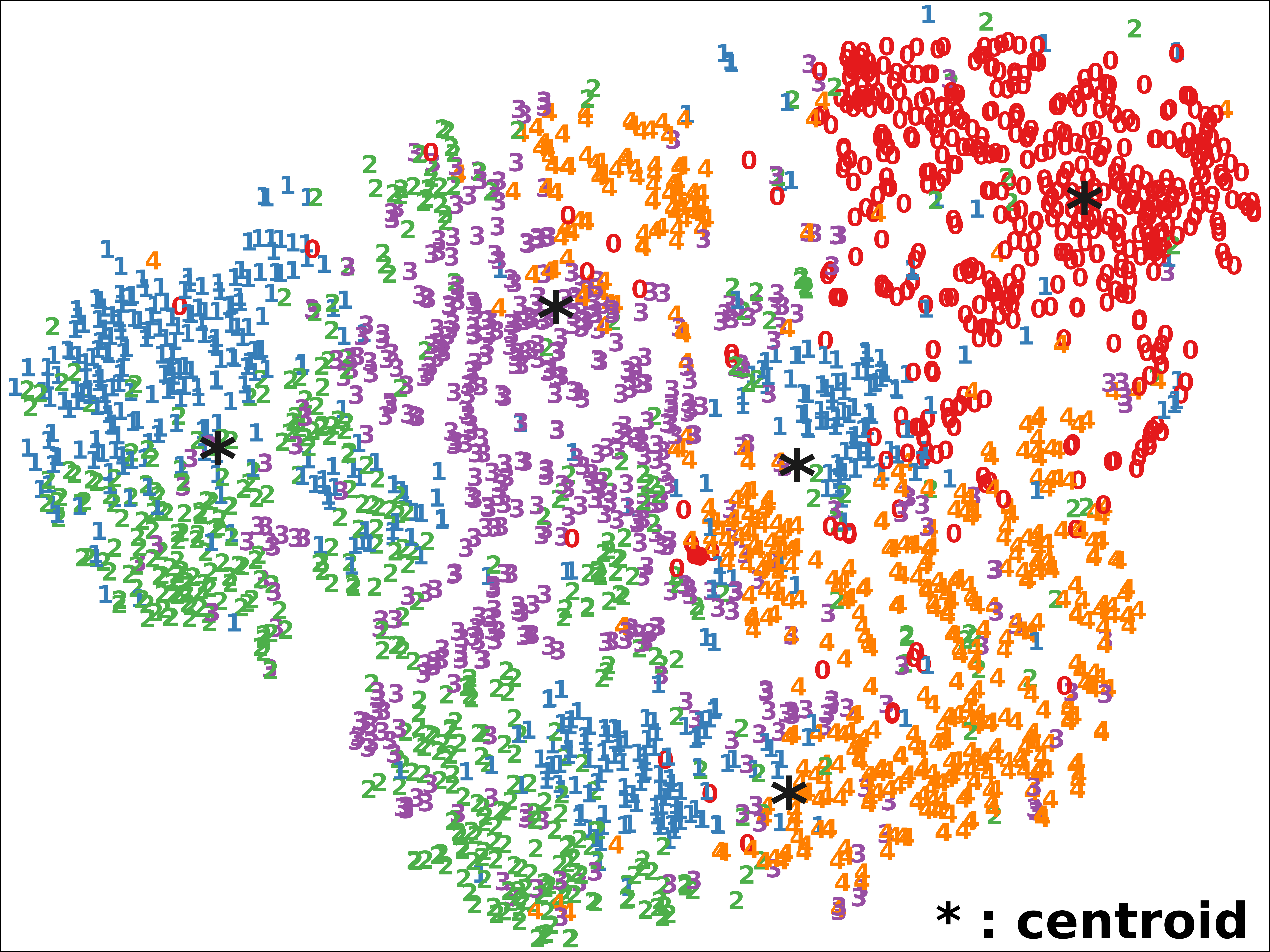
(a) V1-0

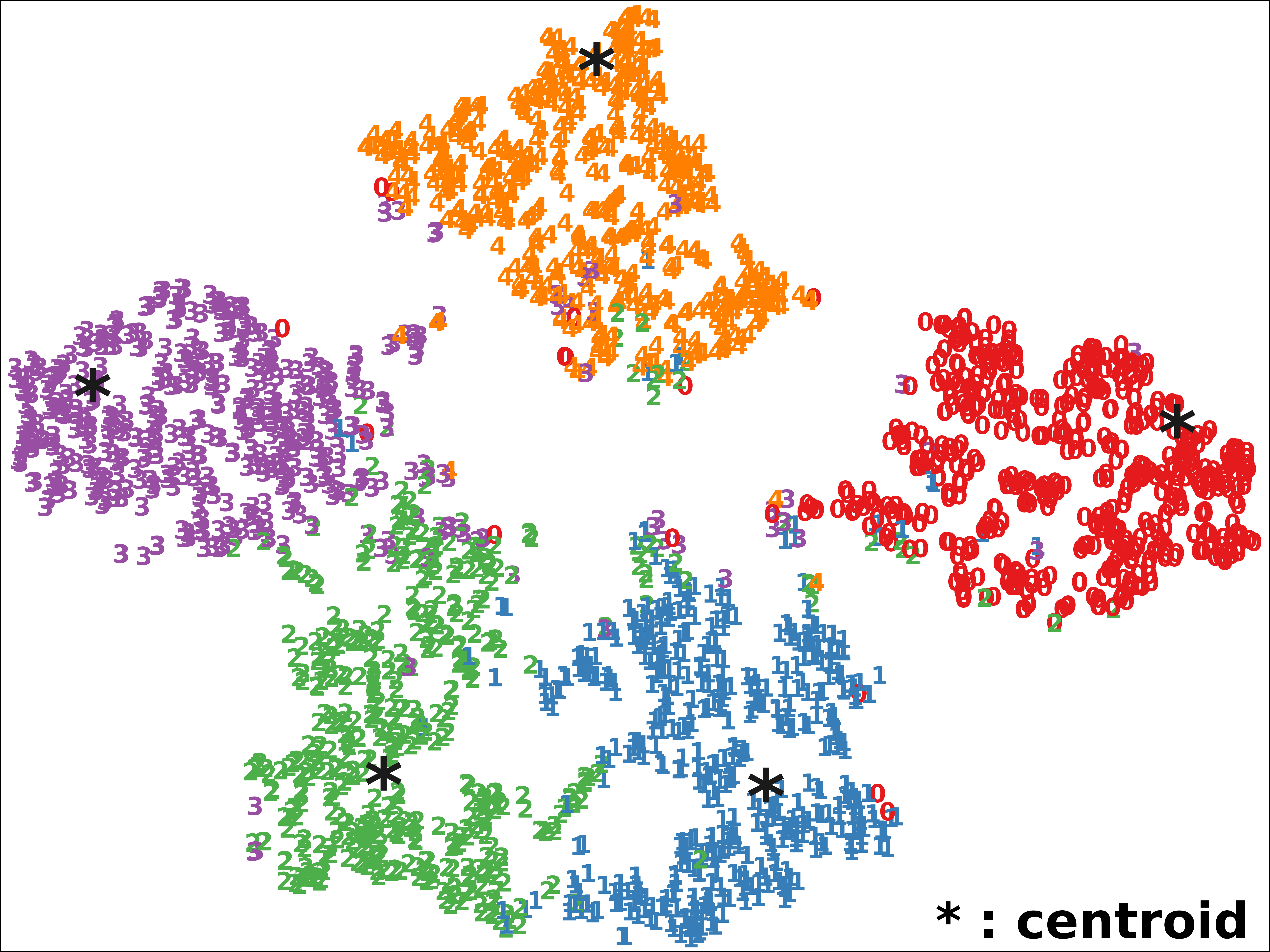
(b) V1-1000

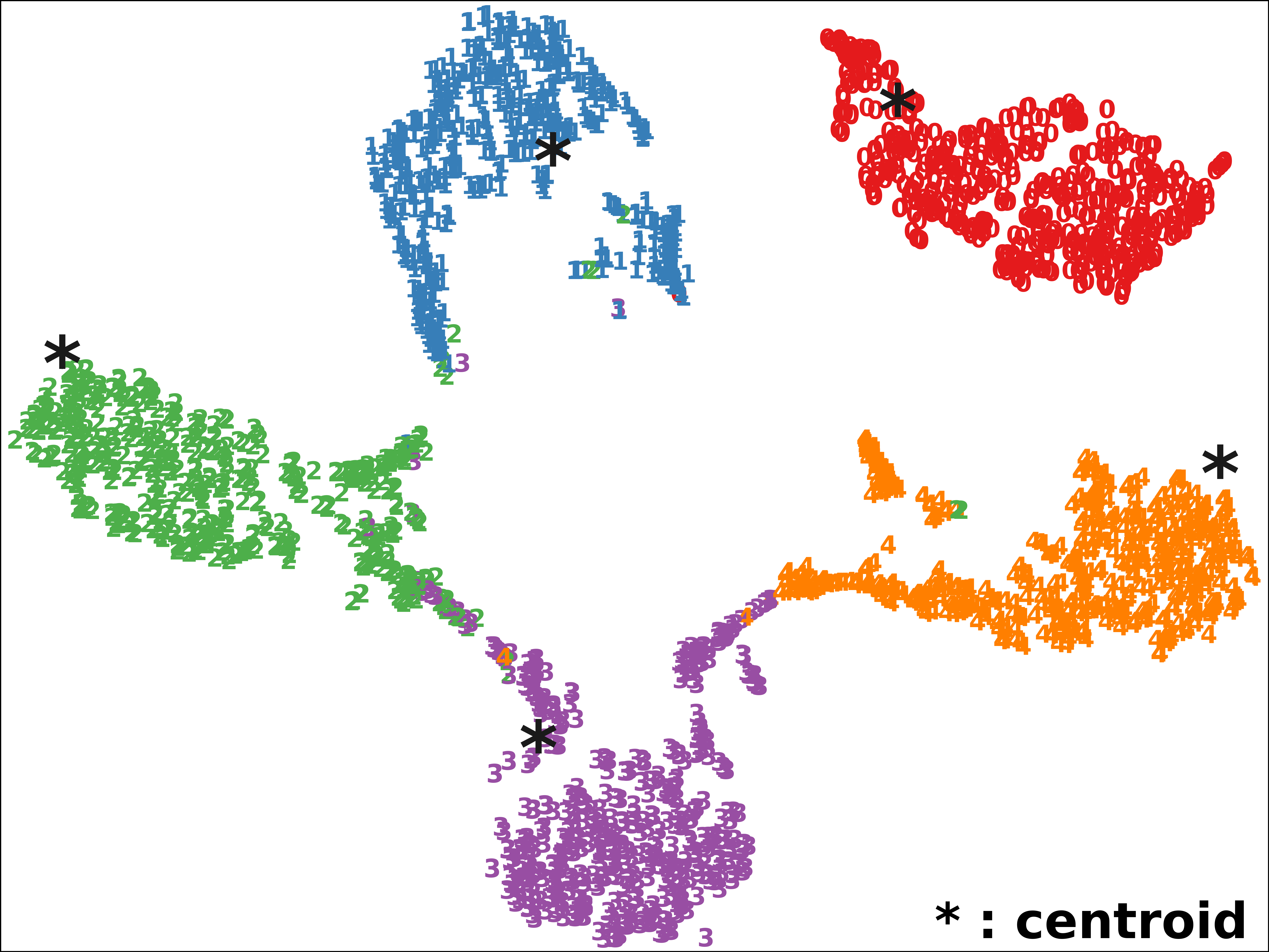
(c) V1-2000

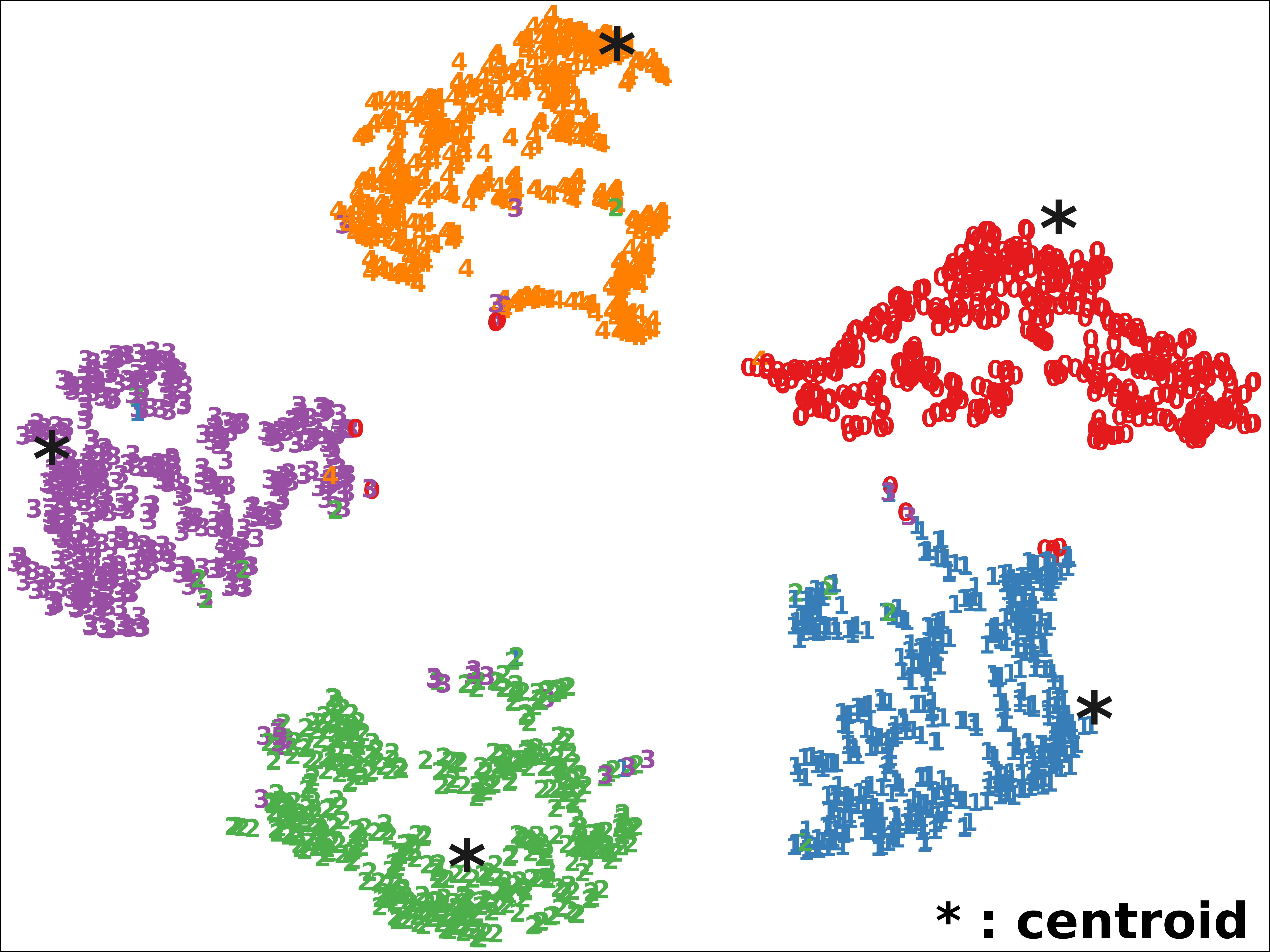
(d) V1-3000

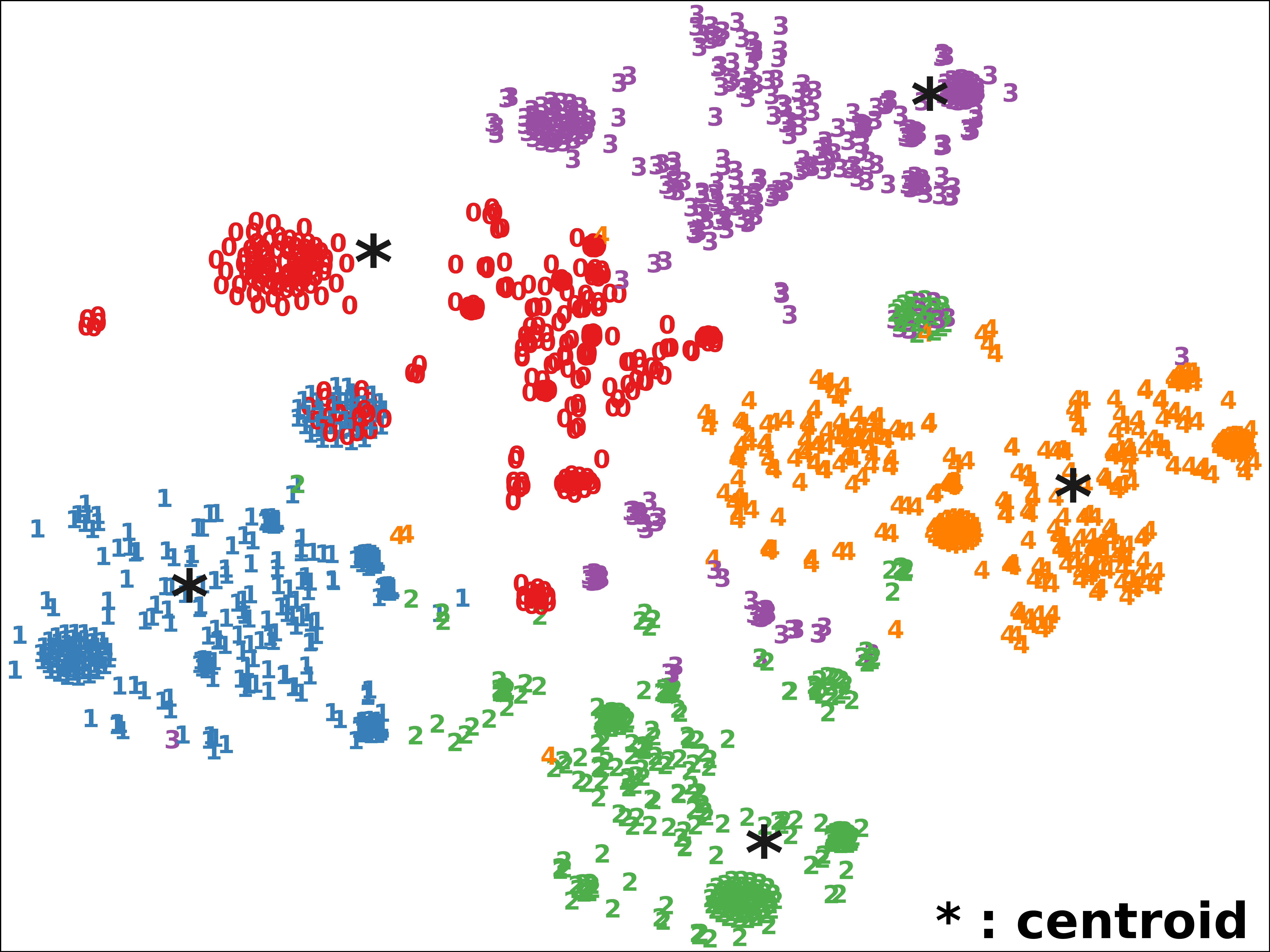
(e) V2-0

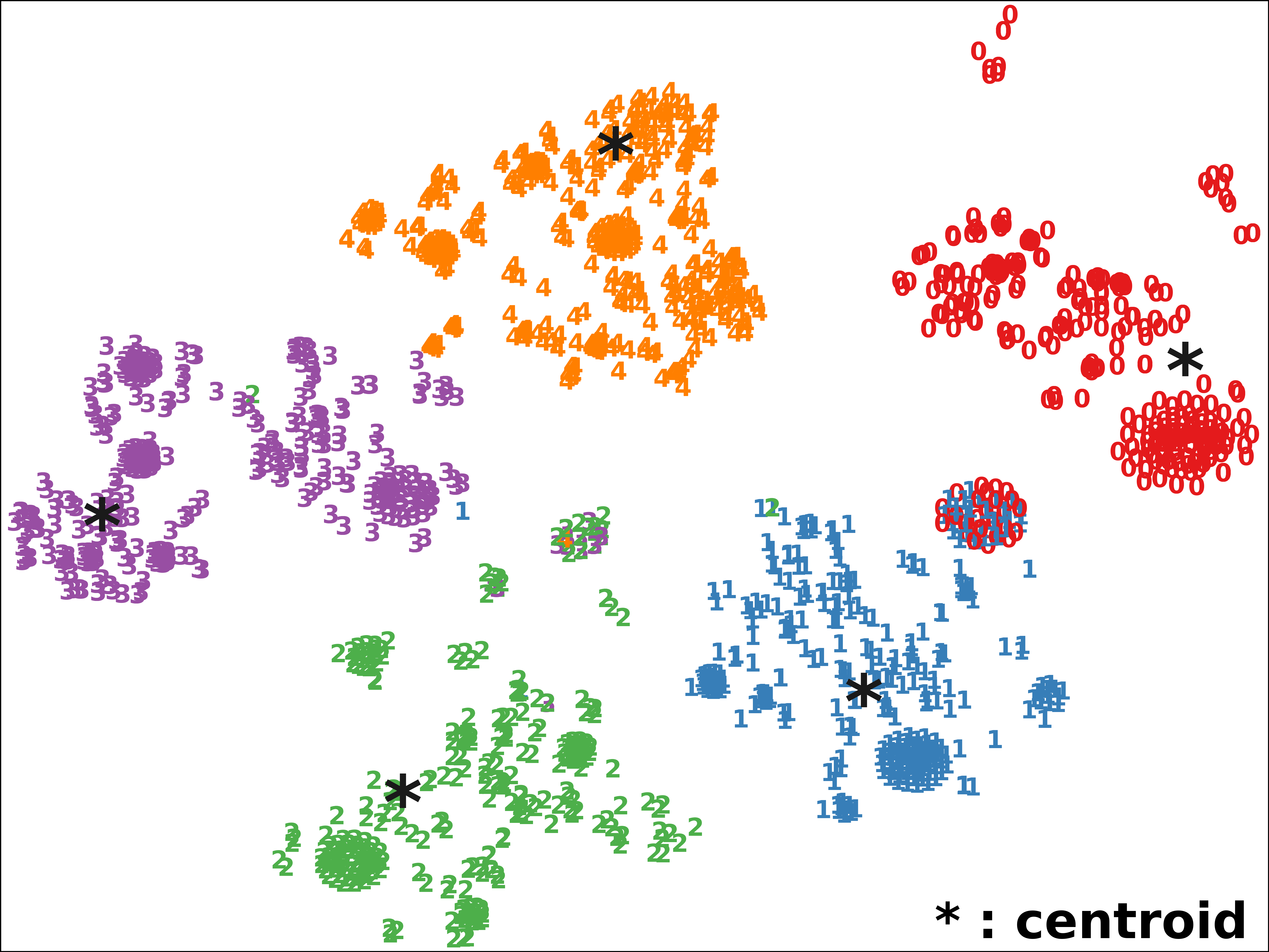
(f) V2-1000

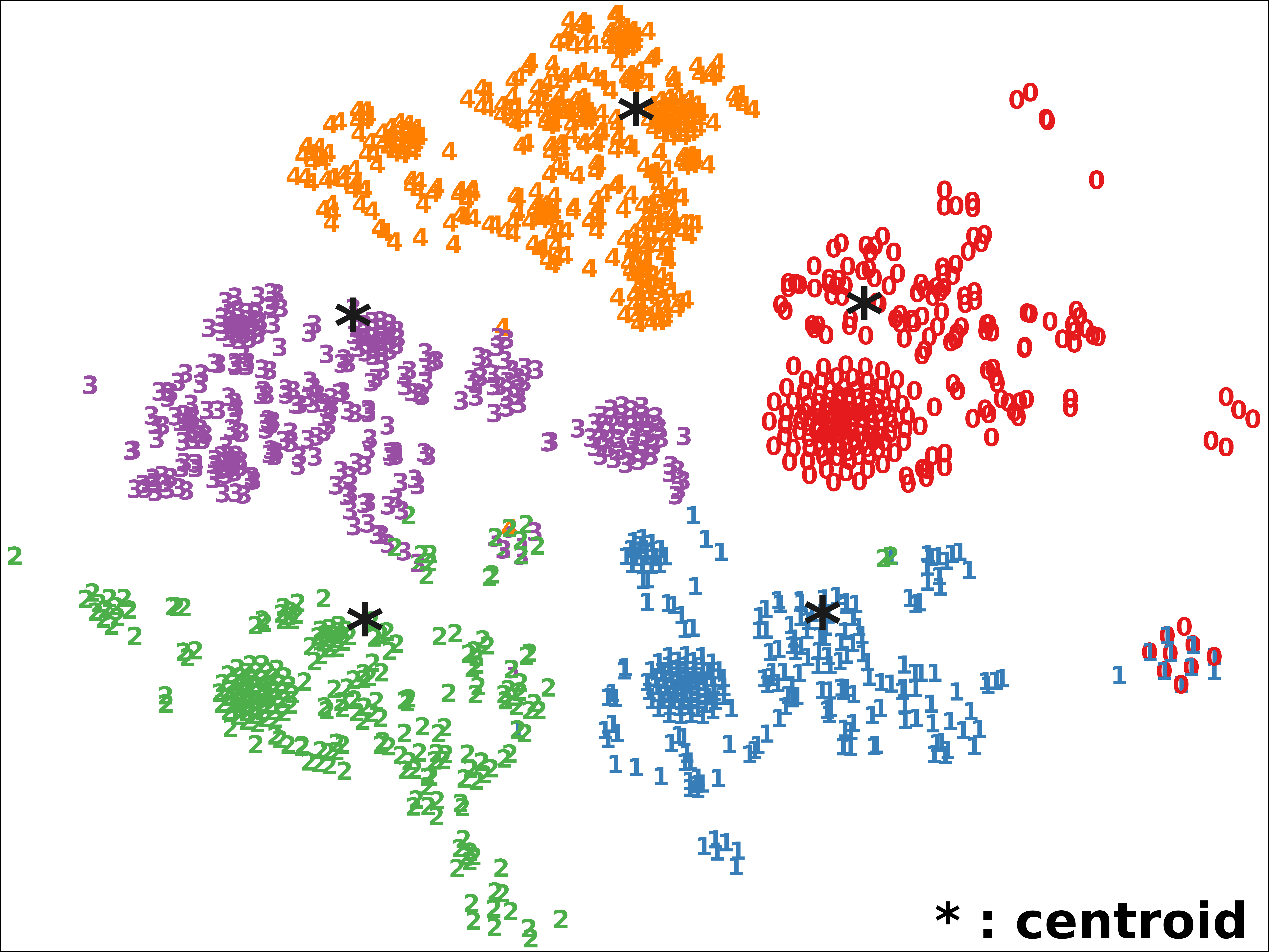
(g) V2-2000

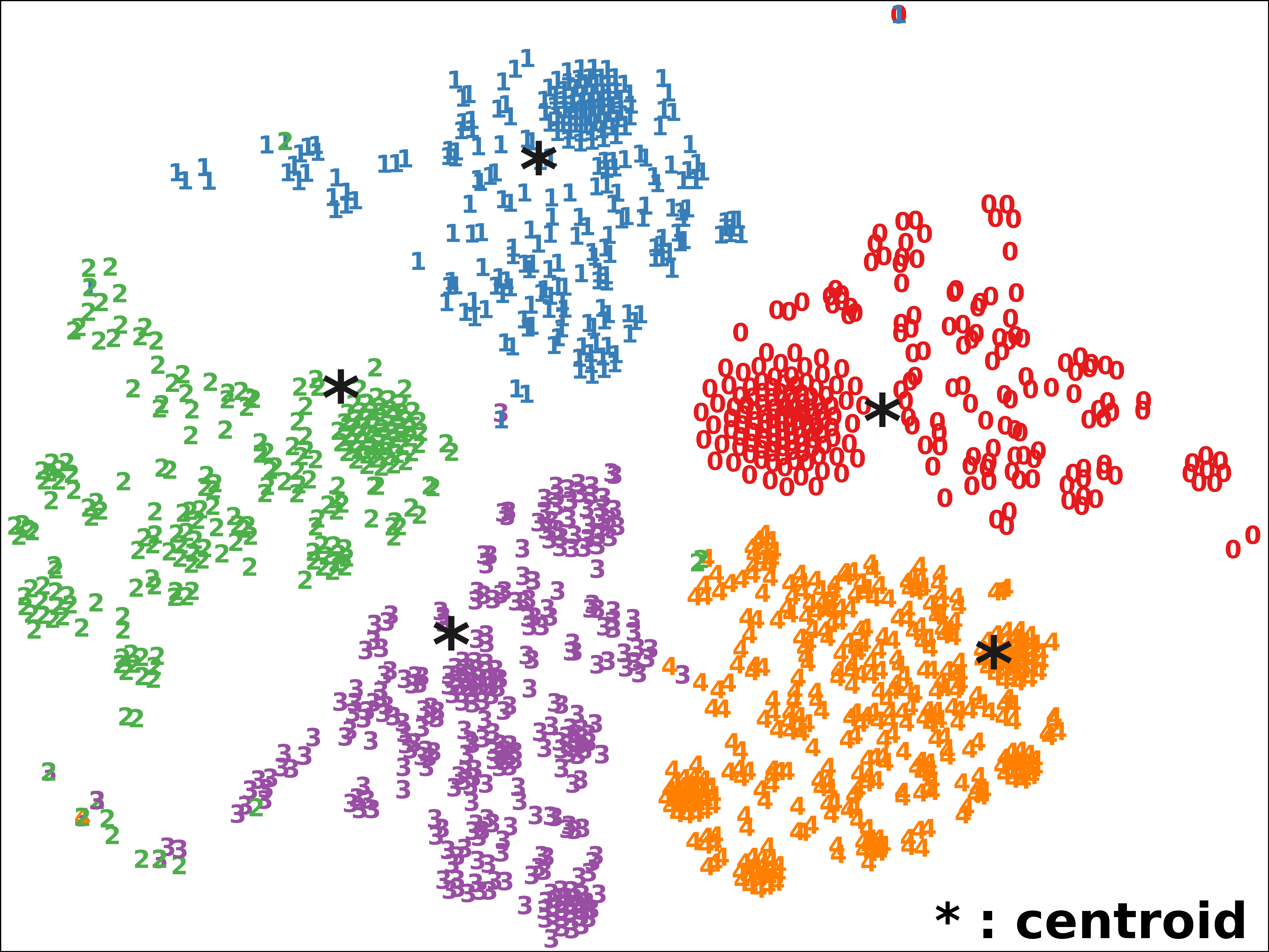
(h) V2-3000

Figure 3: Visualization of embedded features. V1 is BDGP’ visual features and V2 is BDGP’ textual features. (a) and (e) show the embedded features when pre-training is finished. The numbers represent batches that have been trained in the following discriminative feature learning.

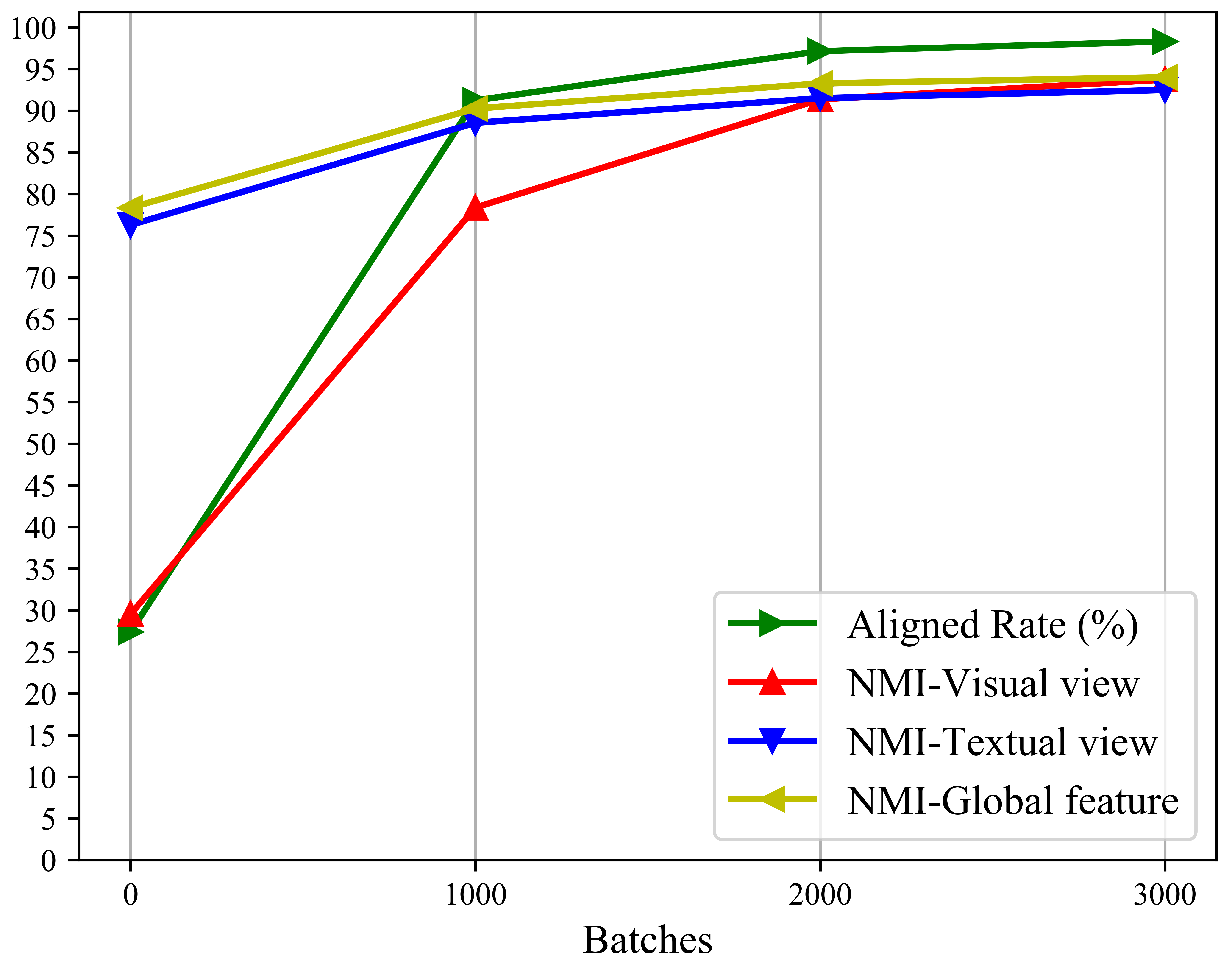
(a) Aligned Rate and NMI

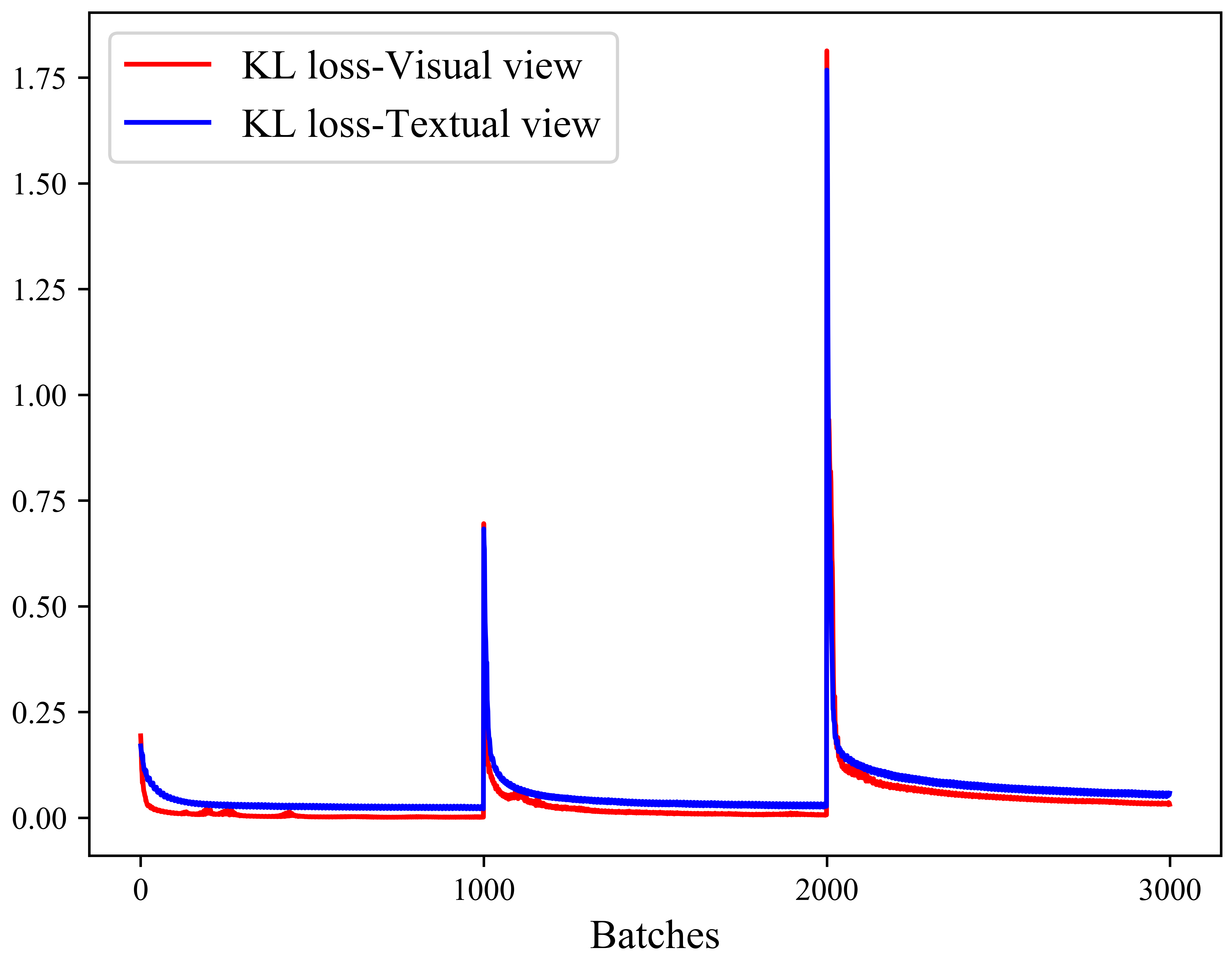
(b) Clustering (KL) loss

Figure 4: Model analysis. The training process on BDGP.

We conduct model analysis on BDGP dataset. In Fig. 4(a), we can find that Aligned Rate and clustering performance are positively correlated. In Fig. 4(b), each time the target distribution is updated, the newly generated and enhanced pseudo soft assignments have stronger discriminability. So, the clustering loss (i.e., KL divergence) values suddenly increase. Then the soft cluster assignments of all views are trained to be consistent due to the unified target distribution, which improves the Aligned Rate of the multiple views’ predictions.

In Fig. 3, we visualize the learning process of embedded features on BDGP via $t$-SNE [41]. The cluster centroids of each view are also plotted, which are the learnable parameters in the clustering layers, i.e., $\{\boldsymbol{\mu}_{j}^{v}\}{{}_{j=1}^{K}}{{}_{v=1}^{V}}$. When the pre-training of autoencoders is finished, two views’ embedded features of BDGP are shown in Fig. 3(a) and (e), respectively. The discriminative degree of features is low and the cluster centroids can not reflect the true clustering structures, corresponding to the low NMI values and low Aligned Rate as shown in Fig. 4(a) (when #Batches = 0). By mining the global discriminative information contained in the two views, SDMVC builds a target distribution to learn more discriminative features, which in turn are used to update the target distribution. Thus in the following feature learning process, the clustering structures of embedded features become clearer and clearer while their centroids are gradually separated, corresponding to the high NMI values and high Aligned Rates.

The above observations verify the mechanism of SDMVC to boost clustering performance, i.e., by performing the proposed multi-view discriminative feature learning, SDMVC can globally utilize the discriminative and complementary information while overcoming the negative impact on clustering caused by some views with unclear clustering structures.

Convergence and Parameter. As shown in Fig. 4(b), the algorithm has good convergence property after each update of the target distribution. Since the Aligned Rate of SDMVC is calculated in an unsupervised manner, we advise stopping training by taking a high value, such as $90\%$, to guarantee the multi-view clustering consistency. The setting of the trade-off coefficient $\gamma$ follows those methods (e.g., [19] and [14]) with a trade-off strategy between clustering and reconstruction, i.e., $\gamma=0.1$. Therefore, SDMVC has no hyper-parameters that need to be carefully tuned.

VI Conclusion

In this paper, we have proposed a novel self-supervised discriminative feature learning framework for deep multi-view clustering (SDMVC). Different from existing MVC methods, SDMVC can overcome the negative impact on clustering performance caused by certain views with unclear clustering structures. In a self-supervised manner, it utilizes the discriminative information from a global perspective to establish a unified target distribution, which is used to learn more discriminative features and consistent predictions of multiple views. Experiments on different types of multi-view datasets demonstrate that the proposed method has achieved state-of-the-art clustering performance. In addition, SDMVC has the complexity that is linear to the data size and thus it has a wide application potential.

References

- [1] Changqing Zhang, Huazhu Fu, Qinghua Hu, Xiaochun Cao, Yuan Xie, Dacheng Tao, and Dong Xu. Generalized latent multi-view subspace clustering. TPAMI, 42(1):86–99, 2018.
- [2] Ming, Yin, Junbin, Gao, Shengli, Xie, and Guo. Multiview subspace clustering via tensorial t-product representation. IEEE Transactions on Neural Networks and Learning Systems, pages 851–864, 2019.
- [3] Y. Xie, J. Liu, Y. Qu, D. Tao, and L. Ma. Robust kernelized multiview self-representation for subspace clustering. IEEE Transactions on Neural Networks and Learning Systems, PP(99):1–14, 2020.
- [4] J. Guo, Y. Sun, J. Gao, Y. Hu, and B. Yin. Rank consistency induced multiview subspace clustering via low-rank matrix factorization. IEEE Transactions on Neural Networks and Learning Systems, PP(99), 2021.
- [5] Jialu Liu, Chi Wang, Jing Gao, and Jiawei Han. Multi-view clustering via joint nonnegative matrix factorization. In SDM13, pages 252–260. SIAM, 2013.
- [6] Yang Wang, Lin Wu, Xuemin Lin, and Junbin Gao. Multiview spectral clustering via structured low-rank matrix factorization. IEEE Transactions on Neural Networks and Learning Systems, 29(10):4833–4843, 2018.
- [7] Zuyuan Yang, Naiyao Liang, Wei Yan, Zhenni Li, and Shengli Xie. Uniform distribution non-negative matrix factorization for multiview clustering. IEEE transactions on cybernetics, 2020.
- [8] Feiping Nie, Jing Li, and Xuelong Li. Self-weighted multiview clustering with multiple graphs. In IJCAI, pages 2564–2570, 2017.
- [9] Hao Wang, Yan Yang, and Bing Liu. Gmc: Graph-based multi-view clustering. IEEE Transactions on Knowledge and Data Engineering, 32(6):1116–1129, 2019.
- [10] Xi Peng, Zhenyu Huang, Jiancheng Lv, Hongyuan Zhu, and Joey Tianyi Zhou. COMIC: Multi-view clustering without parameter selection. In ICML, pages 5092–5101, 2019.
- [11] Zhaoyang Li, Qianqian Wang, Zhiqiang Tao, Quanxue Gao, and Zhaohua Yang. Deep adversarial multi-view clustering network. In IJCAI, pages 2952–2958, 2019.
- [12] Pengfei Zhu, Binyuan Hui, Changqing Zhang, Dawei Du, Longyin Wen, and Qinghua Hu. Multi-view deep subspace clustering networks. arXiv preprint arXiv:1908.01978, 2019.
- [13] Deyan Xie, Xiangdong Zhang, Quanxue Gao, Jiale Han, Song Xiao, and Xinbo Gao. Multiview clustering by joint latent representation and similarity learning. IEEE transactions on cybernetics, 50(11):4848–4854, 2019.
- [14] Jie Xu, Yazhou Ren, Guofeng Li, Lili Pan, Ce Zhu, and Zenglin Xu. Deep embedded multi-view clustering with collaborative training. Information Sciences, 573:279–290, 2021.
- [15] Qianqian Wang, Jiafeng Cheng, Quanxue Gao, Guoshuai Zhao, and Licheng Jiao. Deep multi-view subspace clustering with unified and discriminative learning. IEEE Transactions on Multimedia, 2020.
- [16] Yan Yang and Hao Wang. Multi-view clustering: A survey. Big Data Mining and Analytics, 1(2):83–107, 2018.
- [17] Yang Wang. Survey on deep multi-modal data analytics: Collaboration, rivalry, and fusion. ACM Transactions on Multimedia Computing, Communications, and Applications (TOMM), 17:1–25, 2021.
- [18] Junyuan Xie, Ross Girshick, and Ali Farhadi. Unsupervised deep embedding for clustering analysis. In ICML, pages 478–487, 2016.
- [19] Xifeng Guo, Long Gao, Xinwang Liu, and Jianping Yin. Improved deep embedded clustering with local structure preservation. In IJCAI, pages 1753–1759, 2017.
- [20] Kamran Ghasedi Dizaji, Amirhossein Herandi, Cheng Deng, Weidong Cai, and Heng Huang. Deep clustering via joint convolutional autoencoder embedding and relative entropy minimization. In ICCV, pages 5736–5745, 2017.
- [21] Xifeng Guo, En Zhu, Xinwang Liu, and Jianping Yin. Deep embedded clustering with data augmentation. In ACML, pages 550–565, 2018.
- [22] Yazhou Ren, Kangrong Hu, Xinyi Dai, Lili Pan, Steven CH Hoi, and Zenglin Xu. Semi-supervised deep embedded clustering. Neurocomputing, 325:121–130, 2019.
- [23] Yuan Xie, Bingqian Lin, Yanyun Qu, Cuihua Li, Wensheng Zhang, Lizhuang Ma, Yonggang Wen, and Dacheng Tao. Joint deep multi-view learning for image clustering. IEEE Transactions on Knowledge and Data Engineering, 2020.
- [24] Bo Yang, Xiao Fu, Nicholas D Sidiropoulos, and Mingyi Hong. Towards k-means-friendly spaces: Simultaneous deep learning and clustering. In ICML, pages 3861–3870, 2017.
- [25] Yazhou Ren, Ni Wang, Mingxia Li, and Zenglin Xu. Deep density-based image clustering. Knowledge-Based Systems, 197:105841, 2020.
- [26] Ruihuang Li, Changqing Zhang, Huazhu Fu, Xi Peng, Tianyi Zhou, and Qinghua Hu. Reciprocal multi-layer subspace learning for multi-view clustering. In ICCV, pages 8172–8180, 2019.
- [27] Qinghai Zheng, Jihua Zhu, Zhongyu Li, Shanmin Pang, Jun Wang, and Yaochen Li. Feature concatenation multi-view subspace clustering. Neurocomputing, 379:89–102, 2020.
- [28] Mansheng Chen, Ling Huang, Chang-Dong Wang, and Dong Huang. Multi-view clustering in latent embedding space. In AAAI, pages 3513–3520, 2020.
- [29] Handong Zhao, Zhengming Ding, and Yun Fu. Multi-view clustering via deep matrix factorization. In AAAI, pages 2921–2927, 2017.
- [30] Shudong Huang, Zenglin Xu, Ivor W Tsang, and Zhao Kang. Auto-weighted multi-view co-clustering with bipartite graphs. Information Sciences, 512:18–30, 2020.
- [31] Chang Tang, Xinwang Liu, Xinzhong Zhu, En Zhu, Zhigang Luo, Lizhe Wang, and Wen Gao. Cgd: Multi-view clustering via cross-view graph diffusion. In AAAI, pages 5924–5931, 2020.
- [32] Zhenglai Li, Chang Tang, Xinwang Liu, Xiao Zheng, Guanghui Yue, Wei Zhang, and En Zhu. Consensus graph learning for multi-view clustering. IEEE Transactions on Multimedia, 2021.
- [33] Yang Wang, Wenjie Zhang, Lin Wu, Xuemin Lin, Meng Fang, and Shirui Pan. Iterative views agreement: An iterative low-rank based structured optimization method to multi-view spectral clustering. In IJCAI, pages 2153–2159, 2016.
- [34] Shaohua Fan, Xiao Wang, Chuan Shi, Emiao Lu, Ken Lin, and Bai Wang. One2multi graph autoencoder for multi-view graph clustering. In Proceedings of The Web Conference 2020, pages 3070–3076, 2020.
- [35] Zheng Zhang, Li Liu, Fumin Shen, Heng Tao Shen, and Ling Shao. Binary multi-view clustering. TPAMI, 41(7):1774–1782, 2018.
- [36] Yazhou Ren, Shudong Huang, Peng Zhao, Minghao Han, and Zenglin Xu. Self-paced and auto-weighted multi-view clustering. Neurocomputing, 383:248–256, 2020.
- [37] Runwu Zhou and Yi-Dong Shen. End-to-end adversarial-attention network for multi-modal clustering. In CVPR, pages 14607–14616, 2020.
- [38] Xiukun Sun, Miaomiao Cheng, Chen Min, and Liping Jing. Self-supervised deep multi-view subspace clustering. In ACML, pages 1001–1016, 2019.
- [39] Siwei Wang, Xinwang Liu, En Zhu, Chang Tang, Jiyuan Liu, Jingtao Hu, Jingyuan Xia, and Jianping Yin. Multi-view clustering via late fusion alignment maximization. In IJCAI, pages 3778–3784, 2019.
- [40] Daniel J. Trosten, Sigurd Løkse, Robert Jenssen, and Michael Kampffmeyer. Reconsidering representation alignment for multi-view clustering. In CVPR, 2021.
- [41] Laurens van der Maaten and Geoffrey Hinton. Visualizing data using t-sne. JMLR, 9:2579–2605, 2008.
- [42] James MacQueen. Some methods for classification and analysis of multivariate observations. In Proceedings of the 5th Berkeley Symposium on Mathematical Statistics and Probability, pages 281–297, 1967.
- [43] Yann LeCun, Léon Bottou, Yoshua Bengio, and Patrick Haffner. Gradient-based learning applied to document recognition. Proceedings of the IEEE, 86(11):2278–2324, 1998.
- [44] Han Xiao, Kashif Rasul, and Roland Vollgraf. Fashion-mnist: a novel image dataset for benchmarking machine learning algorithms. arXiv preprint arXiv:1708.07747, 2017.
- [45] Xiao Cai, Hua Wang, Heng Huang, and Chris Ding. Joint stage recognition and anatomical annotation of drosophila gene expression patterns. Bioinformatics, 28(12):i16–i24, 2012.
- [46] Li Fei-Fei, Rob Fergus, and Pietro Perona. Learning generative visual models from few training examples: An incremental bayesian approach tested on 101 object categories. In CVPR, pages 178–178. IEEE, 2004.
- [47] Andrew Y Ng, Michael I Jordan, and Yair Weiss. On spectral clustering: Analysis and an algorithm. In NeurIPS, pages 849–856, 2002.
- [48] Zhenyu Huang, Peng Hu, Joey Tianyi Zhou, Jiancheng Lv, and Xi Peng. Partially view-aligned clustering. NeurIPS, 33, 2020.
- [49] Xavier Glorot, Antoine Bordes, and Yoshua Bengio. Deep sparse rectifier neural networks. In JMLR, pages 315–323, 2011.
- [50] Diederik P Kingma and Jimmy Ba. Adam: A method for stochastic optimization. arXiv preprint arXiv:1412.6980, 2014.