InsertGNN: A Hierarchical Graph Neural Network for the TOEFL Sentence Insertion Problem

Abstract

Sentence insertion is an interesting NLP problem but received insufficient attention. Existing approaches in sentence ordering, text coherence, and question answering are neither suitable nor good enough at solving it. To bridge this gap, we propose InsertGNN, a simple yet effective model that represents the problem as a graph and adopts a hierarchical graph neural network (GNN) to learn the connection between sentences. We evaluate our method in our newly collected TOEFL dataset and further verify its effectiveness on the larger arXiv dataset using cross-domain learning. Extensive experiments demonstrate that InsertGNN outperforms all baselines by a large margin with an accuracy of 70%, rivaling the average human test scores.

1 Introduction and Related Work

Sentence insertion first described by Barzilay and Lapata (2008), is usually regarded as an essential task to evaluate the linguistic ability of humans. However, after the emergence of deep learning, it has drawn little interest during the past decade compared to other NLP topics such as machine translation and text generation. Consequently, there is no ’canonical’ deep learning-based solution specifically designed for this problem. To bridge this gap, we construct a dataset from TOEFL  (see an example in Appendix A), an English proficiency test with full records of examinees’ accuracy scores, and investigate whether current NLP techniques are capable of outperforming the non-native speakers.

Sentence ordering and question answering (QA) are the two most closely-related sub-fields to sentence insertion. On the one hand, as a more general case of sentence insertion, sentence ordering first employs a pair-wise order ranking via multi-layer perceptrons (MLPs) (Chen et al., 2016). But this ranking can introduce severe error propagation. To alleviate that issue, the pointer network (PN) is adopted (Gong et al., 2016), where the attention mechanism is subsequently added to enhance the model capability (Logeswaran et al., 2016; Cui et al., 2018). Nevertheless, the PN architecture cannot be directly used in sentence insertion due to their distinct inputs. Putra and Tokunaga (2017) design an unsupervised graph method from the perspective of sentence similarities and coherence inside a text, and claim superiority on the supervised Entity Grid (Barzilay and Lapata, 2008) and the unsupervised Entity Graph (Guinaudeau and Strube, 2013). But it is non-parametric and requires building all graphs with potential positions of the taken-out sentence. On the other hand, QA provides a more universal solution for our case (Devlin et al., 2018; Joshi et al., 2020; Yang et al., 2019; Yamada et al., 2020). The taken-out sentence and the paragraph can be regarded as the question and context respectively, which are then linearly combined and fed into a network to output the position. But this linear combination presents a problem for state-of-the-art models like Transformers (Vaswani et al., 2017) in terms of understanding the inner logic between the new concatenated paragraph and its slots.

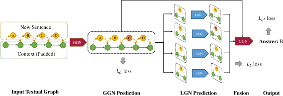
Figure 1: The architecture of our proposed InsertGNN.

In this paper, we represent the sentence insertion problem as a directed graph, where each node stands for a sentence and the edge depicts their relative potential order. This pattern imitates the way that people tackle sentence insertion, i.e., putting the new sentence into each slot and checking the coherence. Moreover, we introduce a novel global-local fused GNN dubbed InsertGNN with delicately designed components to extract both global and local semantic information. In order to verify its efficacy, we conduct thorough experiments in the TOEFL dataset with and without cross-domain learning. The results convincingly corroborate that InsertGNN surpasses all baselines and can achieve competent performance in comparison to human examinees.

2 Methodology

2.1 Preliminary

The input paragraph is first split into five parts as $\{c_{1},c_{2},...,c_{5}\}$ according to four different slots, i.e., $A,B,C,D$. We pad the paragraph to make the graph complete if there is no leading sentence before the slot $A$ or no ending sentence after the slot $D$. Then a graph $\mathcal{G}=(\mathcal{V},\mathcal{E})$ (see Fig. 1) is built to describe all potential orders of the inserted sentence, where each node $v_{i}$ represents a sentence and the directed edge $e_{ij}$ represents the relative order. If two sentences are or possibly are connected, there is a directed edge between them.

After that, we feed all five sentences $\{c_{1},c_{2},...,c_{5}\}$ from the splitted context paragraph and the taken-out sentence $q$ into a sentence encoder, obtaining representation vectors $\{\mathbf{S}_{c_{1}},...,\mathbf{S}_{c_{5}}\}$ and $\mathbf{S}_{q}$. These vectors serve as node features, where $\mathbf{S}_{q}$ corresponds to features of node $\{A,B,C,D\}$.

2.2 Global Graph Attention Networks

Contextual semantics play a vital role in the determination of insertion positions. To begin with, we apply an $L$-layer Global Graph Attention Network (GGN) (Veličković et al., 2017) to aggregate this global contextual information. The input feature is formulated as:

$$\mathbf{H}^{0}=\{\underbrace{\mathbf{S}_{c1},...,\mathbf{S}_{c5}}_{\rm paragraph},\underbrace{\mathbf{S}_{q},\mathbf{S}_{q},\mathbf{S}_{q},\mathbf{S}_{q}}_{\rm slots}\}.$$ (1)

Then for a center node $i$ and its neighbor $j$, the attention score at layer $l$ is computed as:

$$e_{ij}=\rho(\alpha^{T}\cdot(\mathbf{W}\mathbf{H}_{i}^{l}\oplus\mathbf{W}\mathbf{H}_{j}^{l})),$$ (2)

where $\rho$ is the activation function and $\mathbf{W}$ is a trainable parameter. The attention weight is obtained by softmax as $\alpha_{ij}=\frac{\exp{e_{ij}}}{\Sigma_{k\in N_{i}}{(\exp{e_{ik}}})}$. After that, $\alpha_{ij}$ are used to update node features as:

$$\mathbf{H}^{l}_{i}=\sigma(\Sigma_{j\in N_{i}}\alpha_{ij}\mathbf{H}^{l-1}_{j}\mathbf{W}^{l}).$$ (3)

The representations for four slots in the last layer $\{\mathbf{H}_{A}^{L},\mathbf{H}_{B}^{L},\mathbf{H}_{C}^{L},\mathbf{H}_{D}^{L}\}$ are forwarded into an MLP shared by the global-local fusion stage to get prediction $\hat{y}$. Then for a batch with $N$ samples, the binary cross-entropy (BCE) loss is calculated as:

$$L_{G}=-\frac{1}{N}\sum_{i=0}^{N}[\hat{y}\log{y}+(1-\hat{y})\log{(1-y)}],$$ (4)

where $y\in\{0,1\}$ is the ground truth label.

2.3 Local Graph Convolutional Networks

However, GGN is insensitive to local details (Zhang et al., 2020). Undeniably, the answer sometimes can be concluded by immediately reading the two sentences nearby the slot rather than the whole paragraph. Toward this goal, we utilize a Local Graph Network (LGN) to concentrate on the local sentence interactions (see Fig. 2).

To be concise, we create four subgraphs with only the slot and its two surrounding sentences, whose features are the output of the previous GGN. The subgraphs are then fed into an $M$-layer parameter-shared GCN (Kipf and Welling, 2016), which is followed by a Weisfeiler-Lehman (WL) algorithm (Weisfeiler and Leman, 1968) to extract the multi-scale sub-tree features. The output of each layer $\mathbf{Z}^{m}$ is treated as WL’s fingerprint. Similar to DGCNN (Phan et al., 2018), we horizontally concatenate these fingerprints $\{\mathbf{Z}^{1},...,\mathbf{Z}^{M}\}$ rather than calculating the WL graph kernel. Then we apply a $4\times 4$ size pooling along with a fully-connected layer for subgraph classification. Finally, we compute the BCE loss $L_{L}$ for these four subgraphs.

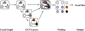
Figure 2: The illustration of LGN layers..

2.4 Global-local Fusion

At the fusion stage, $\mathbf{H}^{L}$ and $\mathbf{Z}^{M}$ are combined together to integrate both global and local information. We take a mean value of $\mathbf{Z}^{M}$ if node $i$ is contained in more than one subgraph. The fused features $\mathbf{E}=\mathbf{H}^{L}+{\rm mean}(\mathbf{Z}^{M})$ go through another GGN, and the output for four slots is fed into the shared MLP to attain the final prediction $\hat{y}^{\prime}$, which is used during the inference period. After that, a BCE loss $L_{G^{\prime}}$ is computed, and the total loss is the sum of three BCE losses as $L=\alpha L_{G}+\beta L_{L}+\gamma L_{G^{\prime}}$, where $\alpha$, $\beta$ and $\gamma$ are loss weights of $L_{G}$, $L_{L}$ and $L_{G^{\prime}}$.

3 Experiment

3.1 Training Configurations

We use Sentence Transformer (Reimers and Gurevych, 2019) as the sentence encoder to summarize the content of sentences, which makes sentences with similar meanings close in vector space. It is first trained on Natural Language Inference (NLI) and then fine-tuned on the Semantic Textual Similarity benchmark (STSb) train set. Furthermore, we use BERT (Devlin et al., 2018) and its two variants DistillBERT (Sanh et al., 2019) and RoBERTa (Liu et al., 2019) for QA architecture. Notably, we neither fine-tune the baseline Transformers nor the Sentence Transformer, and only use them as an embedding layer. More experimental details can be found in Appendix C.

3.2 Dataset

TOEFL exams.

TOEFL is one of the largest exams to test the English level of non-native speakers hosted by the Educational Testing Service (ETS) globally. We choose it for two main reasons. First, all TOEFL questions are extracted from academic articles, designed by language experts and therefore are high quality. Second, ETS annually offers score data reports of examinees. According to the latest summary , the average accuracy in the reading section is 70.67%.

Every year ETS releases merely a few articles in TOEFL Practice Online, which prevents us from building a large-scale dataset. We collect all questions since 2011 and got 156 samples with a relatively equal label distribution of 32%, 25%, 22%, and 21%.

ArXiv abstracts.

We construct another dataset from arXiv to enrich the training samples, and choose the abstract as the contextual paragraph, since it is independently readable and well-edited with strong logic clues. We abandon abstracts containing less than 5 sentences or 300 words to keep them more informative. Besides, we partially abandon categories that are not in the TOEFL scope. Moreover, several categories have tremendous mathematical formulations. These terms have no meaningful corresponding pretrained embeddings and should not be included in our supplementary dataset. After those selections, 5965 abstracts remain.

NLTK (Loper and Bird, 2002) is used to break the paragraph into sentences and randomly choose one as the sentence to be inserted. Then three other positions are selected to form a TOEFL-like problem. This operation can be repeated multiple times for each abstract since there are dozens of nonredundant combinations. The key statistics of these two datasets are listed in Appendix A.

3.3 Baselines

Unsupervised text coherence model.

Putra and Tokunaga (2017) propose three algorithms to build coherence graphs. The major difference is the determination of edges (see Appendix B).

In the Preceding Adjacent Vertex (PAV), a weighted directed edge is established from each sentence to the preceding adjacent sentence. Single Similarity Vertex (SSV) discards the constraints of precedence and adjacency. Multiple Similar Vertex (MSV) even relaxes the singular condition and allows multiple outgoing edges for each sentence as long as their corresponding similarity score exceeds a threshold $\theta$. In the experiment, we use the same sentence encoder as our InsertGNN for the graph instead of GloVe (Pennington et al., 2014).

Topological sort.

Rather than framing the sentence ordering as a sequence prediction problem, Prabhumoye et al. (2020) regard it as a constraint learning problem. Sentences between two slots are represented as nodes with a known constraint between them. An MLP is used to predict the remaining constraints of the relative order between the taken-out sentence and other sentences.  Lai et al. (2021) extend Sentence-Entity Graph Recurrent Network (SE-GRN) (Yin et al., 2019) and utilize two graph-based classifiers to iteratively conduct pairwise predictions for pairwise sentences.

QA methods.

Here we formulate two kinds of QA architectures. The P-type (Plain) linearly combines the dependent sentence and the paragraph as the input and extracts the output vector of the [CLS] character as the final representation. The A-type (Altered) puts the new sentence into all four possible slots and classifies those differently filled paragraphs. The final prediction will be the one with the highest probability.

3.4 Results

TOEFL.

We test the unsupervised text coherence model first. PAV attains the highest accuracy of 41.66$\%$ on our TOEFL dataset (see Table  1), in accord with Putra and Tokunaga (2017)’s evaluation. It indicates that local cohesion is more important than long-distance cohesion, in line with our motivation for LGNs.

Method	Acc_TOEFL (%)
PAV	41.66
SSV	34.62
MSV	37.18

Table 1: Unsupervised learning accuracy. The best and the second best are in bold and underlined, respectively.

Next, we test the performance of supervised approaches with different validation proportions. The result shows our InsertGNN observably improves upon other baselines in all cases, reaching the highest accuracy of 71.5$\%$ (see Table  2). It is comparable to the average human accuracy of 70.67$\%$, suggesting our model can do at least as well as non-native English speakers. We also conduct an ablation study to examine the contribution of each loss in Appendix D.

Method		Acc_TOEFL (%) (dev=0.05)	Acc_TOEFL (%) (dev=0.5)
BERT	P	42.86	38.46
	A	42.86	32.05
DistillBERT	P	57.14	35.89
	A	57.14	29.49
RoBERTa	P	42.86	35.89
	A	42.86	28.61
Topological Sort		57.14	34.62
SE-GRN		57.14	46.15
InsertGNN		71.43	55.12

Table 2: Supervised learning accuracy under different validation split ratios of 0.05 and 0.5. P and A refers to the P-type and the A-type QA structure.

From ArXiv to TOEFL.

We further evaluate InsertGNN using cross-domain learning. Specifically, models are first trained on the arXiv dataset (source domain) with a validation splitting ratio of 0.05 and then directly tested on the TOEFL dataset (target domain). InsertGNN still stands out with an accuracy of 39.1$\%$ (see Table  3).

Method		Acc_arXiv (%)	Acc_TOEFL (%)
BERT	P	34.74	33.97
	A	32.63	30.13
DistillBERT	P	35.22	33.97
	A	31.33	30.76
RoBERTa	P	33.56	32.69
	A	3255	3141
Topological Sort		43.62	28.85
SE-GRN		44.96	36.53
InsertGNN		46.31	39.10

Table 3: Cross-domain learning accuracy from the arXiv dataset to the TOEFL dataset. The left and right columns correspond to the accuracy in the arXiv test set and the whole TOEFL dataset, respectively.

The accuracy in TOEFL is generally lower than in arXiv, because the contents of the two datasets are slightly different. ArXiv abstracts are a brief summarization and therefore very condensed. In contrast, the TOEFL paragraphs are an expanded narrative of a sub-point or a detailed explanation, which is more elaborate with a stronger inner logic. This manner of writing causes a decrease in accuracy when models are cross-domain.

4 Conclusion and Future Work

In the paper, we propose a novel sentence insertion framework called InsertGNN and build a benchmark dataset from TOEFL. Strong empirical evidence demonstrates the effectiveness of InsertGNN in this specific NLP task. It surpasses the unsupervised text coherence methods, the topological sort approach, and existing QA models. We offer a new perspective to solve problems that can be depicted using the graph structure.

Limitations

Despite the superior performance of our model, there are still some limitations left for future work. Most importantly, the TOEFL sentence insertion is of small data size. Though we offer a compensatory dataset curated from the arXiv abstracts, more efforts need to be paid to collecting a larger and high-quality sentence insertion dataset.

Appendix A Details of Datasets

There we give an example of the sentence insertion problem in the TOEFL efficiency test (see Table 4).

Context Paragraph	[A] The age of rock art in Australia has been revised several times, with earlier dates suggested recently after new discoveries. [B] Accurate scientific proof has dated the first appearance of surface rock in Australia to approximately 30,000 to 50,000 years ago. [C] This lengthy and astounding history of rock art in Australia makes it the oldest art tradition known today in the world. [D]
New Sentence	Thanks to radiocarbon dating and technological development in studying evidence, researchers can now give a more precise age on this type of art.
Answer	[B] is the correct answer. Here, we need to match back “this type of art” to what it is referencing in order to correctly place the prompt sentence. It’s referencing rock art, named in the first sentence, making the answer [B].

Table 4: An example of TOEFL sentence insertion problem. It is extracted from questions of the third reading passage named "Rock Art of the Australia Aborigines" from TOEFL Practice Online 23.

In the experiments, we use two sorts of datasets, one is the collected TOEFL dataset, and the other is the arXiv abstract dataset. We summarize their statistics of them in Table 5.

Dataset	Size	Sentences	Words	Topics
TOEFL	156	7.31	133.94	Anthropology, Architecture, Astronomy, Economics, Biology, Chemistry, Communication, North America, Physics, Political Science, Psychology Sociology, World History
arXiv	5965	7.24	121.36	Astrophysics, Computer Vision and Pattern Recognition, Cryptography, Economics, General Relativity High Energy Physics-Theory, Information Theory, Networking and Internet Architecture, Quantum Physics

Table 5: Dataset statistics, including the sample size, average number of sentences inside each paragraph, the average number of words of each paragraph, and their main topics (categories).

Appendix B Some Baseline Models

There we provide a visualization of how unsupervised text coherence method (Putra and Tokunaga, 2017) processes the sentence insertion problem in Fig. 3.

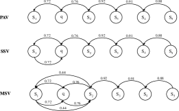
Figure 3: Three graph construction algorithms. PAV only allows edges between a sentence and its preceding sentence. SSV allows edges between a sentence and any other sentences. MSV allows multiple edges.

Appendix C Experimental Details

There we explicitly describe the experimental configurations. All learnable models are trained on a single A100 GPU. Regarding MSV, we choose a threshold $\theta$ of 0.3. For both GGN and LGNs, we utilize the leaky Relu and Relu as the activation function, respectively, and include the dropout mechanism between layers with a 0.5 dropout rate. They both have 1 hidden layer and 4 hidden units. For GGN, we choose 16 hidden attention heads and 4 output attention heads with an attention dropout of 0.6 and a 0.2 negative slope of leaky Relu. They all have a residual connection. For all MLPs, we utilize Tanh as the activation function with no dropout. We adopt an Adam optimizer with a weight decay rate of 0.0005 and a random seed of 1234. After a grid search algorithm, we set $\alpha=0.2$, $\beta=0.2$ and $\gamma=1.0$, where $L_{G^{\prime}}$ is given more weights so that the model can focus more on the global-local fusion information. We train 100 epochs for InsertGNN with a learning rate of 0.0001 and 200 epochs for BERT-based models with a learning rate of 0.01.

Appendix D Additional Results

We implement ablation studies in TOEFL dataset with a validation split ratio of 0.5 to verify the contributions of each constituent of our InsertGNN in Table 6. It can be observed that the LGN significantly promotes the model performance.

	$L_{G}$	$L_{L}$	$L_{G^{\prime}}$	Accuracy
1	✓	-	-	0.4487
2	✓	✓	-	0.5256
3	✓	✓	✓	0.5512

Table 6: Supervised learning accuracy under different validation split ratios of 0.05 and 0.5. P and A refers to the P-type and the A-type QA structure.

References

- Barzilay and Lapata (2008) Regina Barzilay and Mirella Lapata. 2008. Modeling local coherence: An entity-based approach. Computational Linguistics, 34(1):1–34.
- Chen et al. (2016) Xinchi Chen, Xipeng Qiu, and Xuanjing Huang. 2016. Neural sentence ordering. arXiv preprint arXiv:1607.06952.
- Cui et al. (2018) Baiyun Cui, Yingming Li, Ming Chen, and Zhongfei Zhang. 2018. Deep attentive sentence ordering network. In Proceedings of the 2018 Conference on Empirical Methods in Natural Language Processing, pages 4340–4349.
- Devlin et al. (2018) Jacob Devlin, Ming-Wei Chang, Kenton Lee, and Kristina Toutanova. 2018. Bert: Pre-training of deep bidirectional transformers for language understanding. arXiv preprint arXiv:1810.04805.
- Gong et al. (2016) Jingjing Gong, Xinchi Chen, Xipeng Qiu, and Xuanjing Huang. 2016. End-to-end neural sentence ordering using pointer network. arXiv preprint arXiv:1611.04953.
- Guinaudeau and Strube (2013) Camille Guinaudeau and Michael Strube. 2013. Graph-based local coherence modeling. In Proceedings of the 51st Annual Meeting of the Association for Computational Linguistics (Volume 1: Long Papers), pages 93–103.
- Joshi et al. (2020) Mandar Joshi, Danqi Chen, Yinhan Liu, Daniel S Weld, Luke Zettlemoyer, and Omer Levy. 2020. Spanbert: Improving pre-training by representing and predicting spans. Transactions of the Association for Computational Linguistics, 8:64–77.
- Kipf and Welling (2016) Thomas N Kipf and Max Welling. 2016. Semi-supervised classification with graph convolutional networks. arXiv preprint arXiv:1609.02907.
- Lai et al. (2021) Shaopeng Lai, Ante Wang, Fandong Meng, Jie Zhou, Yubin Ge, Jiali Zeng, Junfeng Yao, Degen Huang, and Jinsong Su. 2021. Improving graph-based sentence ordering with iteratively predicted pairwise orderings. arXiv preprint arXiv:2110.06446.
- Liu et al. (2019) Yinhan Liu, Myle Ott, Naman Goyal, Jingfei Du, Mandar Joshi, Danqi Chen, Omer Levy, Mike Lewis, Luke Zettlemoyer, and Veselin Stoyanov. 2019. Roberta: A robustly optimized bert pretraining approach. arXiv preprint arXiv:1907.11692.
- Logeswaran et al. (2016) Lajanugen Logeswaran, Honglak Lee, and Dragomir Radev. 2016. Sentence ordering and coherence modeling using recurrent neural networks. arXiv preprint arXiv:1611.02654.
- Loper and Bird (2002) Edward Loper and Steven Bird. 2002. Nltk: the natural language toolkit. arXiv preprint cs/0205028.
- Pennington et al. (2014) Jeffrey Pennington, Richard Socher, and Christopher D Manning. 2014. Glove: Global vectors for word representation. In Proceedings of the 2014 conference on empirical methods in natural language processing (EMNLP), pages 1532–1543.
- Phan et al. (2018) Anh Viet Phan, Minh Le Nguyen, Yen Lam Hoang Nguyen, and Lam Thu Bui. 2018. Dgcnn: A convolutional neural network over large-scale labeled graphs. Neural Networks, 108:533–543.
- Prabhumoye et al. (2020) Shrimai Prabhumoye, Ruslan Salakhutdinov, and Alan W Black. 2020. Topological sort for sentence ordering. arXiv preprint arXiv:2005.00432.